A new framework for constrained optimization via feedback control of Lagrange multipliers

Abstract

The continuous-time analysis of existing iterative algorithms for optimization has a long history. This work proposes a novel continuous-time control-theoretic framework for equality-constrained optimization. The key idea is to design a feedback control system where the Lagrange multipliers are the control input, and the output represents the constraints. The system converges to a stationary point of the constrained optimization problem through suitable regulation. Regarding the Lagrange multipliers, we consider two control laws: proportional-integral control and feedback linearization. These choices give rise to a family of different methods. We rigorously develop the related algorithms, theoretically analyze their convergence and present several numerical experiments to support their effectiveness concerning the state-of-the-art approaches.

Keywords – Constrained optimization, continuous-time dynamical systems, feedback control, Lagrange multipliers, proportional-integral control, feedback linearization.

1 Introduction

First-order iterative algorithms are prevalent in convex/non-convex optimization and machine learning, primarily to deal with large-scale datasets and leverage parallel architectures. Iterative algorithms for optimization are discrete-time (DT) dynamic systems that update the estimate of the optimization variables at each step. Their continuous-time (CT) counterparts, obtained by considering infinitesimal step sizes, are differential equations whose analysis may provide a deeper theoretical understanding, e.g., on stability and convergence rate.

A paradigmatic example is the gradient flow, defined by the equation $\dot{x}=-\nabla f(x)$, where $f:\mathbb{R}^{n}\to\mathbb{R}$ is a differentiable, unconstrained cost function to be minimized. Gradient flow is the CT version of gradient descent and proximal minimization algorithms via forward and backward Euler discretization, respectively; see, e.g., [25, Sec. 4.1.1]. The study of gradient flow is relevant, e.g., in deep learning, where gradient descent methods have practical success for training but poor theoretical understanding; see, e.g., [27, 10] and references therein. Moreover, works [29, 23] propose CT analysis of Nesterov accelerations for gradient descent.

In this work, we consider the more challenging problem of constrained optimization. In this context, substantial work focuses on CT methods based on Lagrange multipliers, particularly primal-dual methods; we refer the reader to [20, Chapter 15] for a general review. The primary CT approach to constrained optimization is the primal-dual gradient dynamics (PDGD), introduced in [17, 2]. In [26], the authors study the exponential stability of PDGD in the minimization of strongly convex, smooth cost functions with linear equality constraints. The analysis is extended to non-smooth composite optimization in [9, 8], by using a proximal augmented Lagrangian and to non-convex stochastic optimization in [7]. As to convex composite optimization with linear equality constraints, the work [11] illustrates a CT model for the alternating direction method of multipliers (ADMM [5]). We also notice that an antecedent line of research proposes a modification of the gradient flow to envisage equality constraints; the key idea is to build the descent direction $\dot{x}$ as a combination of a projected gradient and of a Gauss-Newton direction, which drives the solution toward the feasible set; see, e.g., [30, 28, 31]. Finally, works [28, 31, 26] envisage inequality constraints as well by extending first-order conditions to Karush-Kuhn-Tucker (KKT) conditions [20].

This brief review highlights that most of the literature proposes the CT analysis of existing algorithms without developing novel CT algorithms for optimization. In contrast, this work proposes a new CT framework for convex and non-convex constrained optimization. In particular, we focus on equality constraints. The proposed framework leverages a feedback control perspective: we start from the solution of first-order necessary conditions for minima and build a CT dynamic system whose control input is the vector of the Lagrange multipliers. The output represents the constraints which we regulate accordingly. Several control laws are suitable for the Lagrange multipliers to achieve the desired regulation; this gives rise to a family of control-based first-order methods. In particular, this work focuses on two methods: proportional-integral (PI) control and feedback linearization.

The first contribution of this work is the development and analysis of the proposed control-theoretic framework. The second contribution is the specialization to specific control laws and the theoretical analysis of their convergence. Moreover, we illustrate several numerical experiments that validate the effectiveness of the method beyond the theoretical conditions of convergence. Particular attention is devoted to the comparison with state-of-the-art algorithms.

We organize the paper as follows. In Section 2, we formulate the problem, review the theory of Lagrange multipliers and describe the proposed control-theoretic framework. The two succeeding sections specialize the framework to two possible control strategies. Specifically, Section 3 develops the PI control method, proves its convergence and analyzes the convergence rate for strongly convex problems with linear constraints. Section 4 develops the feedback linearization method and the proof of its convergence for possibly non-convex problems. Section 5 illustrates several numerical experiments that demonstrate the practical effectiveness of the proposed methods in different applications. Finally, Section 6 concludes the paper.

2 Problem statement and proposed framework

We consider the constrained optimization problem

$$\begin{split}\min_{x\in\mathbb{R}^{n}}&\,f(x)\\ &\rm{s.t.}\\ &h(x)=0\end{split}$$ (1)

where $f:\mathbb{R}^{n}\mapsto\mathbb{R}$ and $h:\mathbb{R}^{n}\mapsto\mathbb{R}^{m}$ are differentiable, possibly non-convex functions.

The Lagrangian of problem (1) is

$$\mathcal{L}(x,\lambda)=f(x)+\lambda^{\top}h(x)$$ (2)

where $\lambda\in\mathbb{R}^{m}$ is the vector of Lagrange multipliers. We report the following well-known theorem for self-consistency; see, e.g., [20, Sec 11.3] for a complete overview.

Theorem 1 (First-order necessary conditions).

Let $x^{\star}\in\mathbb{R}^{n}$ be a local minimum of $f$ such that $h(x^{\star})=0$. Then, there exists a unique $\lambda^{\star}\in\mathbb{R}^{m}$ such that $(x^{\star},\lambda^{\star})$ is a saddle point of $\mathcal{L}(x,\lambda)$, i.e,

$$\nabla f(x^{\star})+J_{h}(x^{\star})^{\top}\lambda^{\star}=0$$ (3)

where $J_{h}(x)\in\mathbb{R}^{m,n}$ is the Jacobian matrix of $h$ evaluated in $x$.

In the rest of the paper, we call stationary point any couple $(x^{\star},\lambda^{\star})$, with $x^{\star}\in\mathbb{R}^{n}$ and $\lambda^{\star}\in\mathbb{R}^{m}$, which satisfies (3) and the constraints, i.e.,

$$\begin{split}&\nabla f(x^{\star})+J_{h}(x^{\star})^{\top}\lambda^{\star}=0\\ &h(x^{\star})=0.\end{split}$$ (4)

In this work, we focus on first-order algorithms, i.e., on methods that achieve stationary points. In the non-convex case, finding a stationary point does not guarantee local optimality; however, the literature is rich in first-order methods in large-scale optimization and machine learning thanks to their low complexity concerning, e.g., second-order methods, which require computing and storing Hessian matrices as well; see, e.g., [3, 20, 12].

2.1 Proposed framework: feedback control of Lagrange multipliers

In this subsection, we illustrate the proposed framework to find a stationary point of problem (1) by building a suitable CT dynamic system with controlled Lagrange multipliers.

Let us define the dynamic system $\mathcal{P}$ with state $x(t)\in\mathbb{R}^{n}$, input $\lambda(t)\in\mathbb{R}^{m}$ and output $y(t)\in\mathbb{R}^{m}$, described by the equations

$$\mathcal{P}:\left\{\begin{split}\dot{x}(t)&=-\nabla f(x(t))-J_{h}(x(t))^{\top}\lambda(t)\\ y(t)&=h(x(t))\end{split}\right.$$ (5)

The following result holds.

Lemma 1.

An equilibrium point $(x^{\star},\lambda^{\star})$ of $\mathcal{P}$ is a stationary point of problem (1) if and only if $h(x^{\star})=0$.

Proof.

By definition, an equilibrium point $(x^{\star},\lambda^{\star})$ of $\mathcal{P}$ satisfies equation (3). If $h(x^{\star})=0$, then (4) holds and $(x^{\star},\lambda^{\star})$ is a stationary point to problem (1). Conversely, any stationary point satisfies (4), thus (3), then it corresponds to an equilibrium point $(x^{\star},\lambda^{\star})$ of $\mathcal{P}$ with $h(x^{\star})=0$. ∎

Lemma 1 suggests we can compute a stationary point of problem (1) by designing a suitable input $\lambda(t)$ that drives $\mathcal{P}$ to converge to an equilibrium point and regulates the output to zero. A standard way to approach this regulation problem is to design a suitable feedback controller $\mathcal{K}$. In Fig. 1, we depict a general scheme; $y(t)$ is the feedback signal to the input of $\mathcal{K}$, possibly together with the state of $\mathcal{P}$. We underline that $\mathcal{P}$ is a representation of an optimization algorithm; therefore, the state is known as well as the output, which is different from physical systems where the observation of the state may be critical.

The goal of this work is to tackle the following problem.

Problem 1.

Design a feedback controller $\mathcal{K}$ for $\mathcal{P}$ such that

$$\begin{split}&\lim_{t\to\infty}x(t)=x^{\star},\\ &\lim_{t\to\infty}y(t)=0.\end{split}$$ (6)

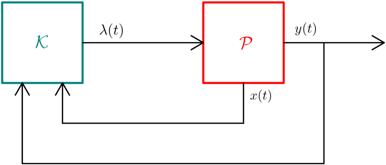
Figure 1: Structure of the proposed feedback control approach. The state and the output of $\mathcal{P}$ defined in (5) are fed back to the controller $\mathcal{K}$, whose output is the vector of the Lagrange multipliers.

In this work, we consider two possible design techniques for $\mathcal{K}$ to solve Problem 1: PI control and feedback linearization.

2.2 Related work

To our knowledge, controlling the Lagrange multipliers in constrained optimization is novel. In the literature, the use of control methods to analyze or develop optimization algorithms is only partly explored.

Regarding first-order unconstrained optimization, the works [19, 13] propose control interpretations of known algorithms such as gradient descent, heavy-ball and Nesterov’s accelerated methods. In particular, they show that these algorithms correspond to DT feedback systems, where the current gradient is the control input. By using integral quadratic constraints, they analyze their convergence. Differently from our work, this framework does not envisage constrained optimization.

A different research line studies the solution of equations via control. In the DT framework, [22] and [21] solve linear algebraic equations using iterative learning control and observer-based controller design, respectively. Instead, in [4], the authors build a CT-controlled system whose output is regulated to solve $g(x)=0$, where $g:\mathbb{R}^{n}\mapsto\mathbb{R}^{n}$ is a vector function. By choosing appropriate control Lyapunov functions, they retrace standard iterative methods, such as Newton-Raphson and conjugate gradient methods, and develop new variants. Unlike our work, this framework considers equality-constrained problems with no cost function to minimize. However, one may argue that finding a stationary point corresponds to solving the first-order equations $(\nabla f(x)+\sum_{i=i}^{m}\lambda_{i}\nabla h_{i}(x))^{\top}$ together with $h(x)=0$ in the variables $x$ and $\lambda$, i.e., a system of dimension $(n+m)\times(n+m)$. In other terms, one can apply the methods proposed in [4] to find the zeros of the vector function $g(x,\lambda)=\left[(\nabla f(x)+\sum_{i=i}^{m}\lambda_{i}\nabla h_{i}(x))^{\top},h(x)^{\top}\right]^{\top}$. However, as summarized in [4, Table 1], this approach gives rise to second-order methods and continuous Newton algorithms, which require the inversion of the Jacobian of $g(x,\lambda)$. Therefore, the numerical complexity is prohibitive for large-scale problems.

Beyond the control-theoretic approach, PDGD [26] is a valuable CT approach to solve problem (1). In the next section, we compare our approach to PDGD.

3 First method: PI control

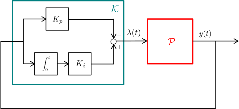
Figure 2: First method: PI control. We feedback the output $y(t)$ to the controller $\mathcal{K}$, which applies proportional an integral actions.

A possible strategy to design $\mathcal{K}$ for Problem 1 is to apply a PI action on $y(t)=h(x(t))$. The PI control is widespread in industrial and engineering applications, thanks to its effectiveness in regulating many processes by tuning two parameters.

In our framework, the PI control law is as follows:

$$\lambda(t)=K_{p}y(t)+K_{i}\int_{0}^{t}y(\tau)\,\rm{d}\tau$$ (7)

where $K_{p}\in\mathbb{R}$ and $K_{i}\in\mathbb{R}$ are the coefficients of the proportional and integral terms, respectively. We depict the corresponding feedback scheme in Fig. 2.

As a consequence, $\mathcal{K}$ is a dynamic system described by the differential equation

$$\begin{split}\dot{\lambda}(t)&=K_{p}\frac{\rm{d}}{\rm{d}t}y(t)+K_{i}y(t)\\ &=K_{p}J_{h}(x(t))\dot{x}(t)+K_{i}y(t).\end{split}$$ (8)

In the following, we drop the variable $t$ in long formulas, namely $x=x(t)$, $\dot{x}=\dot{x}(t)$, $\lambda=\lambda(t)$ and $\dot{\lambda}=\dot{\lambda}(t)$. Given the definition of $\dot{x}$ in (5), the closed-loop dynamics is

$$\begin{split}\dot{x}&=-\nabla f(x)-J_{h}(x)^{\top}\lambda\\ \dot{\lambda}&=-K_{p}J_{h}(x)\left[\nabla f(x)+J_{h}(x)^{\top}\lambda\right]+K_{i}h(x).\end{split}$$ (9)

or, equivalently,

$$\begin{split}\dot{x}&=-\nabla_{x}\mathcal{L}(x,\lambda)\\ \dot{\lambda}&=-K_{p}J_{h}(x)\nabla_{x}\mathcal{L}(x,\lambda)+K_{i}\nabla_{\lambda}\mathcal{L}(x,\lambda).\end{split}$$ (10)

For any equilibrium point $(x^{\star},\lambda^{\star})$, from (9) we get the condition $h(x^{\star})=0$. Therefore, according to Lemma 1, each equilibrium point corresponds to a stationary point in the case of PI control.

Remark 1.

It is worth noticing that by considering a purely integral control, i.e., $K_{p}=0$, we obtain the dynamics

$$\begin{split}\dot{x}&=-\nabla_{x}\mathcal{L}(x,\lambda)\\ \dot{\lambda}&=K_{i}\nabla_{\lambda}\mathcal{L}(x,\lambda).\end{split}$$ (11)

which corresponds to PDGD defined in [26, Eq. (2a)-(2b)], where the symbol $\eta$ is used instead of $K_{i}$. In other words, we can interpret PDGD as applying an integral control to the Lagrange multipliers, which recast PDGD into the proposed control-theoretic framework. In contrast, the proposed PI control extends PDGD to a novel family of CT optimization algorithms.

3.1 Global exponential convergence of PI control method

In this section, by defining a suitable Lyapunov function, we prove that the PI control method is globally exponentially convergent in the convex setting with affine constraints. Moreover, we analyze its convergence rate. We consider the same assumptions as [26], allowing us to compare thoroughly to PDGD.

Assumption 1.

$f$ is strongly convex and twice differentiable.

Assumption 2.

$h$ is affine, i.e., $h(x)=Cx+d$, $C\in\mathbb{R}^{m,n}$, $d\in\mathbb{R}^{m}$. Moreover, $C$ is full rank and there exist $0<\alpha_{1}\leq\alpha_{2}$ such that

$$\alpha_{1}I\preceq CC^{\top}\preceq\alpha_{2}I.$$ (12)

The assumption that $C$ is full rank guarantees that $Cx+d=0$ has solutions and that there are no linearly dependent constraints. We define

$$z(t):=(x(t)^{\top},\lambda(t)^{\top})^{\top}$$ (13)

and

$$z^{\star}:=(x^{\star\top},\lambda^{\star\top})^{\top}$$ (14)

is the equilibrium point of (9), which corresponds to a saddle point of $\mathcal{L}(x,\lambda)$. Assumptions 1 and 2 guarantee the existence and the uniqueness of $z^{\star}$.

According to [26, Lemma 1], there exists a symmetric $B(x)\in\mathbb{R}^{n,n}$ satisfying $\beta_{1}I\preceq B(x)\preceq\beta_{2}I$ for some $0<\beta_{1}<\beta_{2}$ such that

$$\nabla f(x)-\nabla f(x^{\star})=B(x)(x-x^{\star}).$$ (15)

In the following, we write $B=B(x)$ for brevity.

Theorem 2 (Global exponential convergence of PI control method).

Let assumptions 1 and 2 hold. For any $K_{p}>0$, given a constant

$$\rho\geq\frac{K_{p}(\beta_{2}-\beta_{1})^{2}}{2\beta_{1}},$$ (16)

let us set either

$$K_{i}=\rho+K_{p}\beta_{2}~{}\text{ or }~{}K_{i}=\rho+K_{p}\beta_{1}.$$ (17)

Then, there exist real positive constants $c_{1}$ and $c_{2}$ such that

$$\|x(t)-x^{\star}\|_{2}\leq c_{1}e^{-\frac{1}{2}\mu t},~{}~{}~{}\|\lambda(t)-\lambda^{\star}\|_{2}\leq c_{2}e^{-\frac{1}{2}\mu t}$$ (18)

where

$$\mu=\min\left\{K_{p}\alpha_{1},2\beta_{1}-\frac{K_{p}(\beta_{2}-\beta_{1})^{2}}{\rho}\right\}.$$ (19)

Proof.

First of all, we define the candidate Lyapunov function

$$V\big{(}z(t)\big{)}=\big{(}z(t)-z^{\star}\big{)}^{\top}P\big{(}z(t)-z^{\star}\big{)}$$ (20)

where

$$P:=\left(\begin{array}[]{cc}\rho I_{n}&0\\ 0&I_{m}\end{array}\right)\in\mathbb{R}^{m+n,m+n}$$ (21)

for some $\rho>0$. If we prove that

$$\dot{V}\big{(}z(t)\big{)}\leq-\mu V\big{(}z(t)\big{)}$$ (22)

then the theorem statement holds. Therefore, in the following, we focus on conditions that guarantee (22).

We start with some preliminary computations. Since $\nabla_{x}\mathcal{L}(x^{\star},\lambda^{\star})=0$, $\nabla_{\lambda}\mathcal{L}(x^{\star},\lambda^{\star})=0$ and $J_{h}(x)=C$, we have

$$\begin{split}\nabla_{x}\mathcal{L}(x,\lambda)&=\nabla_{x}\mathcal{L}(x,\lambda)-\nabla_{x}\mathcal{L}(x^{\star},\lambda^{\star})\\ &=\nabla f(x)-\nabla f(x^{\star})+J_{h}(x)^{\top}\lambda-J_{h}(x^{\star})^{\top}\lambda^{\star}\\ &=\nabla f(x)-\nabla f(x^{\star})+C^{\top}(\lambda-\lambda^{\star})\end{split}$$ (23)

and

$$\begin{split}\nabla_{\lambda}\mathcal{L}(x,\lambda)&=\nabla_{\lambda}\mathcal{L}(x,\lambda)-\nabla_{\lambda}\mathcal{L}(x^{\star},\lambda^{\star})\\ &=Cx+d-(Cx^{\star}+d)=C(x-x^{\star}).\end{split}$$ (24)

By using (10), (15), (23) and (24), we obtain

$$\begin{split}\dot{z}&(t)=\left(\begin{array}[]{c}\dot{x}(t)\\ \dot{\lambda}(t)\\ \end{array}\right)\\ &=\left(\begin{array}[]{c}-B(x-x^{\star})-C^{\top}(\lambda-\lambda^{\star})\\ K_{i}C(x-x^{\star})-K_{p}C[B(x-x^{\star})+C^{\top}(\lambda-\lambda^{\star})]\end{array}\right)\\ &=\left(\begin{array}[]{cc}-B&-C^{\top}\\ K_{i}C-K_{p}CB&-K_{p}CC^{\top}\end{array}\right)\big{(}z(t)-z^{\star}\big{)}.\end{split}$$ (25)

Let us define

$$G:=\left(\begin{array}[]{cc}-B&-C^{\top}\\ K_{i}C-K_{p}CB&-K_{p}CC^{\top}\end{array}\right)$$ (26)

so that

$$\dot{z}(t)=G\big{(}z(t)-z^{\star}\big{)}.$$

Then,

$$\begin{split}\dot{V}\big{(}z(t)\big{)}&=\dot{z}(t)^{\top}P\big{(}z(t)-z^{\star}\big{)}+\big{(}z(t)-z^{\star}\big{)}^{\top}P\dot{z}(t)\\ &=\big{(}z(t)-z^{\star}\big{)}^{\top}\big{(}G^{\top}P+PG\big{)}\big{(}z(t)-z^{\star}\big{)}.\end{split}$$ (27)

Therefore, a sufficient condition for $\dot{V}\big{(}z(t)\big{)}\leq-\mu V\big{(}z(t)\big{)}$, see (22), is

$$-G^{\top}P-PG-\mu P\succeq 0.$$ (28)

As a consequence, our next goal is to provide sufficient conditions for (28). We compute

$$PG=\left(\begin{array}[]{cc}-\rho B&-\rho C^{\top}\\ K_{i}C-K_{p}CB&-K_{p}CC^{\top}\end{array}\right)$$ (29)

while $G^{\top}P=(PG)^{\top}$. Hence,

$$\begin{split}&-G^{\top}P-PG-\mu P\\ &=\left(\begin{array}[]{cc}2\rho B-\rho\mu I&\left[(\rho-K_{i})I+K_{p}B\right]C^{\top}\\ C\left[(\rho-K_{i})I+K_{p}B\right]&2K_{p}CC^{\top}-\mu I\end{array}\right)\\ &\succeq\left(\begin{array}[]{cc}2\rho B-\rho\mu I&\left[(\rho-K_{i})I+K_{p}B\right]C^{\top}\\ C\left[(\rho-K_{i})I+K_{p}B\right]&K_{p}CC^{\top}\end{array}\right)\end{split}$$ (30)

where the last step holds for $\mu\leq K_{p}\alpha_{1}$. Let us define

$$Q:=(\rho-K_{i})I+K_{p}B\in\mathbb{R}^{n,n}.$$ (31)

Since $CC^{\top}\succ 0$ is invertible from (12) in Assumption 2, we can apply the Schur complement argument: the matrix

$$\left(\begin{array}[]{cc}2\rho B-\rho\mu I&QC^{\top}\\ CQ&K_{p}CC^{\top}\end{array}\right)$$

is positive semidefinite if and only if

$$2\rho B-\rho\mu I-QC^{\top}\frac{1}{K_{p}}(CC^{\top})^{-1}CQ\succeq 0.$$ (32)

Moreover, since $CC^{\top}$ is invertible, then $C^{\top}(CC^{\top})^{-1}C\preceq I$. Therefore, a sufficient condition for (32) is

$$\begin{split}&2\rho B-\rho\mu I-\frac{1}{K_{p}}Q^{2}\succeq 0.\end{split}$$ (33)

As $Q$ depends on $K_{i}$, $K_{p}$ and $\rho$, we can tune these parameters so that (33) holds.

From (31),

$$\left(\rho-K_{i}+K_{p}\beta_{1}\right)I\preceq Q\preceq\left(\rho-K_{i}+K_{p}\beta_{2}\right)I.$$ (34)

For example, if we set either $K_{i}=\rho+K_{p}\beta_{2}$ or $K_{i}=\rho+K_{p}\beta_{1}$ we obtain either $0\succeq Q\succeq K_{p}(\beta_{1}-\beta_{2})I$ or $0\preceq Q\preceq K_{p}(\beta_{2}-\beta_{1})I$, respectively. In both cases, (33) holds if

$$2\rho\beta_{1}-\rho\mu-K_{p}(\beta_{2}-\beta_{1})^{2}\geq 0$$ (35)

which is equivalent to

$$\mu\leq 2\beta_{1}-\frac{K_{p}(\beta_{2}-\beta_{1})^{2}}{\rho}.$$ (36)

From (16), this bound is non-negative. This completes the proof. ∎

Remark 2.

According to (20)-(21), the considered Lyapunov function is

$$V(x,\lambda)=\rho\|x-x^{\star}\|_{2}^{2}+\|\lambda-\lambda^{\star}\|_{2}^{2}.$$

We highlight the role of the parameter $\rho$, which tunes the weight assigned to the terms in $x$ with respect to the terms in $\lambda$. According to Theorem 2, $\rho$ must be lower bounded, i.e., the weight given to the terms in $x$ must be sufficiently large compared to the terms in $\lambda$. We remark that in the convergence proof of PDGD in [26], the Lyapunov function is defined on a non-diagonal matrix $P$, making interpreting the parameters more difficult.

According to [26], PDGD is globally exponentially convergent with rate

$$\mu_{PDGD}=\min\left\{\frac{\eta\alpha_{1}}{4\beta_{2}},\frac{\alpha_{1}\beta_{1}}{4\alpha_{2}}\right\}\leq\frac{\alpha_{1}\beta_{1}}{4\alpha_{2}}.$$ (37)

while for the proposed PI control, the convergence rate $\mu$ is given by (19). The following result holds.

Corollary 1.

If we choose sufficiently large $K_{p}$ and $\rho$, then

$$\mu\approx 2\beta_{1}>\frac{\alpha_{1}\beta_{1}}{4\alpha_{2}}\geq\mu_{PDGD},$$ (38)

i.e., the proposed PI control method has a faster convergence rate with respect to PDGD [26].

In Sec. 5.1, we validate this result about the enhanced convergence speed through numerical simulations.

3.2 Illustrative example

To complete the analysis, we present an example that illustrates how the tuning of $K_{i}$ and $K_{p}$ may affect the convergence rate, and we compare the results to the case $K_{p}=0$, namely PDGD. Let us consider the simple optimization problem

$$\min_{x\in\mathbb{R}}\frac{1}{2}wx^{2}~{}~{}\text{s.t.}~{}~{}~{}x=0$$ (39)

where $w>0$. By applying the PI control, the corresponding closed-loop dynamics is

$$\begin{split}\dot{x}&=-wx-\lambda\\ \dot{\lambda}&=(K_{i}-K_{p}w)x-K_{p}\lambda.\end{split}$$ (40)

This is a second-order CT linear time-invariant system

$$\begin{pmatrix}\dot{x}\\ \dot{\lambda}\end{pmatrix}=\mathrm{A}\begin{pmatrix}x\\ \lambda\end{pmatrix}$$ (41)

with

$$\mathrm{A}:=\left(\begin{array}[]{cc}-w&-1\\ K_{i}-K_{p}w&-K_{p}\end{array}\right).$$ (42)

The eigenvalues of $\mathrm{A}$ are

$$\frac{-(K_{p}+w)\pm\sqrt{(K_{p}+w)^{2}-4K_{i}}}{2}.$$ (43)

For any $K_{i}>0$, the eigenvalues are either real and negative or complex with negative real parts. In particular, if $K_{i}\geq(K_{p}+w)^{2}/4$, $K_{i}$ contributes only to the imaginary part, therefore it does not impact on the convergence rate.

According to the authors of [26], although $\eta>0$ can be arbitrarily large for PDGD, increasing $\eta$ beyond a certain threshold does not lead to faster decaying rate. In our example, if we choose $K_{p}=0$, we obtain PDGD with $\eta=K_{i}$ and, from (43), we see that if $K_{i}\geq w^{2}/4$, then $K_{i}$ has no impact on the real parts of the eigenvalues. This explains the observation in [26].

On the other hand, in the PI control method we can tune $K_{p}>0$ to enhance the convergence rate, provided that the conditions of Theorem 2 are satisfied, which is a benefit with respect to PDGD.

3.3 PI control in non-convex quadratic optimization with linear constraints

To conclude this section, we analyze some properties of the PI control method for quadratic optimization with linear constraints. In particular, we prove that optimization problems exist with non-convex cost functions in which the PI control method converges to a stationary point while PDGD is divergent.

We consider

$$\begin{split}&\min_{x\in\mathbb{R}^{n}}\frac{1}{2}x^{\top}Wx\\ &\text{s.t.}\\ &Cx+d=0\end{split}$$ (44)

where $W\in\mathbb{R}^{n,n}$ is symmetric and $C\in\mathbb{R}^{m,n}$ and $d\in\mathbb{R}^{m}$, with invertible $CC^{\top}$.

Since the cost function is quadratic and the constraints are linear, the closed-loop dynamics with the PI control corresponds to the linear time-invariant system

$$\begin{pmatrix}\dot{x}\\ \dot{\lambda}\\ \end{pmatrix}=\mathrm{A}\begin{pmatrix}x\\ \lambda\\ \end{pmatrix}+\begin{pmatrix}0\\ K_{i}d\\ \end{pmatrix}$$ (45)

with

$$\mathrm{A}:=\begin{pmatrix}-W&-C^{\top}\\ K_{i}C-K_{p}CW&-K_{p}CC^{\top}\end{pmatrix}$$ (46)

Therefore, if $\mathrm{A}$ is Hurwitz, then the system is asymptotically stable, and by construction, the output $y(t)=Cx(t)+d$ is regulated to zero. Thus, for the PI control method, $W$ does not need to be positive definite, i.e., the system does not need to be strongly convex. As an example, let us consider $W=\text{diag}(1,-1)$ and $C=(0,2)$. Since $W$ is indefinite, the quadratic cost function is not convex. The eigenvalues of the corresponding dynamic matrix are $-1$ and $\frac{1-4K_{p}\pm\sqrt{(1-4K_{p})^{2}-16K_{i}}}{2}$. If $K_{p}=0$, all the eigenvalues have positive real part, for all $K_{i}$. In other terms, PDGD is always unstable. Instead, for $K_{p}>\frac{1}{4}$, all the eigenvalues have negative real part for all $K_{i}>0$.

In conclusion, there exist problems with non-convex functions where the PI control method converges to the unique minimum point, as long as we provide a suitable tuning of $K_{p}$. In contrast, PDGD is divergent for any hyperparameter choice. This observation encourages future study of the PI control method in non-convex optimization.

4 Second method: feedback linearization

In this section, we resort to feedback linearization as detailed, e.g., in [14], to design the controller $\mathcal{K}$ introduced in Section 2. Moreover, we study the conditions under which the controlled dynamics is stable, and the algorithm converges to the desired solution.

4.1 Feedback linearization basics

In this subsection, we review some basic concepts of the feedback linearization theory to understand the development of the corresponding controller.

Definition 1.

(Lie derivative, [14, Sec. 1.2], [16, Sec. 13.2]).

Let $F:\mathbb{R}^{n}\mapsto\mathbb{R}^{n}$ be a vector field and $H_{i}:\mathbb{R}^{n}\mapsto\mathbb{R}$. The Lie derivative of $H_{i}$ along $F$ is

$$L_{F}H_{i}(x)=\nabla H_{i}(x)^{\top}F(x)\in\mathbb{R}.$$ (47)

By defining $L_{F}^{0}H_{i}(x)=H_{i}(x)$, for $k=1,2,\dots$, we have

$$L_{F}^{k}H_{i}(x)=(\nabla L_{F}^{k-1}H_{i}(x))^{\top}F(x).$$ (48)

As illustrated, e.g., in [14, 16], feedback linearization can be applied to input-affine nonlinear dynamical systems of the form

$$\begin{split}\dot{x}&=F(x)+G(x)u\\ y&=H(x)\end{split}$$ (49)

where $x(t)\in\mathbb{R}^{n}$, $u(t)\in\mathbb{R}^{m}$, and $y(t)\in\mathbb{R}^{m}$, $F:\mathbb{R}^{n}\mapsto\mathbb{R}^{n}$, $G:\mathbb{R}^{n}\mapsto\mathbb{R}^{n,m}$, $H:\mathbb{R}^{n}\mapsto\mathbb{R}^{m}$. For a dynamical system of this kind, we recall the definition of the relative degree.

Let $G_{j}(x)$ be the $j$-th column of $G(x)$.

Definition 2.

(Relative degree, [14, Sec. 5.1], [16, Sec. 13.2]).

System (49) has a vector relative degree $r=(r_{1},\dots,r_{m})^{\top}$ at $\bar{x}\in\mathbb{R}^{n}$ if

(a) for each $1\leq i,j\leq m$, for each $k=1,\dots,r_{i}-1$, and for all $x$ in a neighbourhood of $\bar{x}$

$$L_{G_{j}}L_{F}^{k}H_{i}(x)=0$$ (50)

and

(b) the matrix $\left[L_{G_{j}}L_{F}^{r_{i}-1}H_{i}(x)\right]_{1\leq i,j\leq m}\in\mathbb{R}^{m,m}$ is nonsingular at $x=\bar{x}$, i.e.,

$$\text{rank}\left(\left[L_{G_{j}}L_{F}^{r_{i}-1}H_{i}(\bar{x})\right]_{1\leq i,j\leq m}\right)=m.$$ (51)

For a single-input, single-output system, if the relative degree is $r$, the output $y$ and its derivatives up to $(r-1)$-th order do not depend on the input, while the $r$-th order derivative does. For linear systems, the concept is equivalent to the relative degree of a transfer function, i.e., the difference between the degree of the denominator and the degree of the numerator.

Now, we recall the concept of zero dynamics.

Definition 3.

(Zero dynamics, [6],[14, Sec. 4.3]). The zero dynamics of a system $\mathcal{S}$ is the dynamical system that describes the internal behavior of $\mathcal{S}$ if we set the initial conditions and the inputs to constrain the output of $\mathcal{S}$ to be identically zero.

In other words, the zero dynamics accounts for the modes that are not observable from the output of the system, whose stability is of concern. We refer the reader to [15] for more insight on this notion.

Finally, we state the non-interacting control problem and its solution.

Definition 4.

(Non-interacting control problem, [14, Sec. 5.3]) Let us consider system (49). We say that a controller of the form

$$u=\alpha(x)+\beta(x)v$$ (52)

with $\alpha(x)\in\mathbb{R}^{m}$, $\beta(x)\in\mathbb{R}^{m,m}$ and $v\in\mathbb{R}^{m}$ solves the non-interacting control problem if in the closed-loop system

$$\left\{\begin{split}\dot{x}&=F(x)+G(x)\alpha(x)+G(x)\beta(x)v\\ y&=H(x)\end{split}\right.$$ (53)

each input $v_{i}$ affects only output $H_{i}$, for each $i=1,\dots,m$.

Theorem 3.

(Non-interacting control solution, [14, Sec. 5.3])

(a) The non-interacting control problem admits a solution if and only if system (49) has some vector relative degree $r$. In that case, the solution is given by

$$\alpha(x)=-A^{-1}(x)b(x),\qquad\beta(x)=A^{-1}(x)$$ (54)

where

$$\begin{split}&A(x)=\left[L_{G_{j}}L_{F}^{r_{i}-1}H_{i}(x)\right]_{1\leq i,j\leq m}\in\mathbb{R}^{m,m}\\ &b(x)=\left[L_{F}^{r_{i}}H_{i}(x)\right]_{i=1,\dots,m}\in\mathbb{R}^{m}.\end{split}$$ (55)

Moreover, for each $i=1,2,\dots,m$, the input-output behavior between $v_{i}(t)$ and $y_{i}(t)$ is linear and described in the $s-$domain by the transfer function

$$\frac{1}{s^{r_{i}}}.$$ (56)

(b) If $v(t)$ stabilizes the system described by (56) and the zero dynamics of (49) is asymptotically stable, then the feedback control system is asymptotically stable.

Part (a) of Theorem 3 provides an input-output global linearization of system (49), which is decoupled in each component $i=1,\dots,m$. From part (b) of Theorem 3, the stability of the controlled system also depends on the zero dynamics, which accounts for the non-observable part of the system.

4.2 Non-interacting control of Lagrange multipliers

In this section, we apply the theory reported in Sec. 4.1 to design a feedback linearized control for the plant $\mathcal{P}$ as defined in (5).

The key point is that $\mathcal{P}$ has the input-affine structure of (49), with

$$\begin{split}F(x)=-\nabla f(x),~{}G(x)=-J_{h}(x)^{\top},~{}H(x)=h(x).\end{split}$$ (57)

Therefore, we can apply Theorem 3 to obtain a decoupled controller if $\mathcal{P}$ has some vector relative degree. Let us analyze this point using the following assumptions.

Assumption 3.

We assume that $m\leq n$, i.e., there are at least as many optimization variables as constraints.

Assumption 4.

We assume that

$$\text{rank}\left(J_{h}(x)\right)=m,\qquad\forall x\in\mathbb{R}^{n}$$ (58)

i.e., the Jacobian of the constraints is always full-rank.

In the case of affine constraints $h(x)=Cx+d=0$, assumptions 3 and 4 guarantee that at least one feasible solution exists. Conversely, in the case of non-convex constraints, assumptions 3 and 4 imply that the feasible set $\Omega=\{x\in\mathbb{R}^{n}:h(x)=0\}$ is an $(n-m)$-dimensional smooth manifold, i.e., locally similar to a $\mathbb{R}^{n-m}$ at all points. Consequently, $\Omega$ is not empty, and we can define a dynamical system whose trajectories evolve onto it, i.e., the zero dynamics. We notice that these assumptions are common in works on dynamical systems approaches to constrained optimization, see, e.g., [28].

Lemma 2.

Under assumptions 3 and 4, the system $\mathcal{P}$ in (5) has a vector relative degree $r=(1,1,\dots,1)^{\top}\in\mathbb{R}^{m}$.

Proof.

Let us consider (49) with (57). For $r_{i}=1$, for each $i=1,\dots,m$, (50) holds. Then, it is sufficient to check (51) to prove the thesis. From (57), $H_{i}(x)=h_{i}(x)$ and $G_{j}(x)=-\nabla h_{j}(x)$. Let us set $r_{i}=1$ in (51). Then,

$$L_{G_{j}}L_{F}^{0}H_{i}(x)=L_{G_{j}}H_{i}(x)=\left(\nabla h_{i}(x)\right)^{\top}\left(-\nabla h_{j}(x)\right).$$ (59)

Thus,

$$\begin{split}&\text{rank}\left(\left[L_{G_{j}}L_{F}^{0}H_{i}(x)\right]_{1\leq i,j\leq m}\right)=\\ \quad&=\text{rank}\left(\left[\left(\nabla h_{i}(x)\right)^{\top}\left(-\nabla h_{j}(x)\right)\right]_{ij}\right)\\ \quad&=\text{rank}\left(-J_{h}(x)J_{h}(x)^{\top}\right)=m.\end{split}$$ (60)

Hence, (51) is satisfied for any $x$. ∎

According to Lemma 2, part (a) of Theorem 3 holds for system (53) with (57). Therefore, we resort to the non-interacting control solution given in Theorem 3. Specifically, we define the static feedback control law

$$\lambda(t)=A(x)^{-1}(-b(x)+v(t))$$ (61)

where $A(x)$ and $b(x)$ are given by (55) with $r_{i}=1$, i.e.,

$$\begin{split}&A(x)=\left[L_{G_{j}}H_{i}(x)\right]_{1\leq i,j\leq m}=-J_{h}(x)J_{h}(x)^{\top}\in\mathbb{R}^{m,m}\\ &b(x)=\left[L_{F}H_{i}(x)\right]_{i=1,\dots,m}=-J_{h}(x)\nabla f(x)\in\mathbb{R}^{m}.\end{split}$$ (62)

By applying the control law (61)-(62), the relationship between the new input $v(t)\in\mathbb{R}^{m}$ and the output $y(t)=h(x(t))\in\mathbb{R}^{m}$ is

$$y_{i}(t)=\int_{0}^{t}v_{i}(\mu)\,{\rm{d}}\mu,~{}~{}~{}i=1,\dots,m,$$ (63)

which is linear and decoupled in each component $i$.

Next, we have to design $v(t)$ to regulate $y(t)$ to zero. A possible solution is to design the controller $\mathcal{G}$ in Fig. 3

$$v(t)=\mathcal{G}(y(t))$$ (64)

such that the closed-loop dynamics is asymptotically stable and $y(t)\to 0$. Given the single integral structure of (63), the simplest way to design $\mathcal{G}$ is to consider $m$ static linear feedback controllers

$$v_{i}(t)=-K_{i}y_{i}(t)$$ (65)

with $K_{i}>0$ for $i=1,\dots,m$. In fact, this leads to

$${y_{i}(t)}=\alpha_{i}e^{-K_{i}t},\quad i=1,\dots,m$$ (66)

where $\alpha_{i}$ is a constant that depends on the initial conditions.

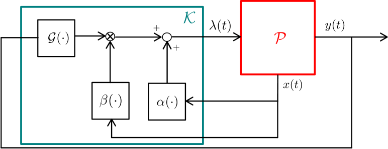
Figure 3: Second method: feedback linearization. We feedback the output $y(t)$ to the controller $\mathcal{K}$ to compute $v(t)$ according to (64), and the state $x(t)$ to compute $u(t)$ according to (52).

To conclude, in Fig. 3, we summarize the feedback control scheme obtained via feedback linearization.

4.3 Local convergence

In this section, we analyze the convergence of the feedback linearization method.

First of all, we notice that closed-loop dynamics (53)-(57)-(64) designed through feedback linearization converges to the feasible set $\Omega$ by construction. To prove the pointwise convergence, let us introduce the second-order sufficient conditions.

Definition 5.

(Second-order sufficient conditions). For problem (1), let $H_{xx}\mathcal{L}(x,\lambda)$ be the Hessian matrix of $\mathcal{L}(x,\lambda)$ with respect to $x$. We say that the second-order sufficient conditions hold at $(x^{\star},\lambda^{\star})$ if

$$v^{\top}H_{xx}\mathcal{L}(x^{\star},\lambda^{\star})v>0$$ (67)

for any $v\in\mathbb{R}^{n}$ such that $J_{h}(x^{\star})v=0$.

If the second-order sufficient conditions hold, $x^{\star}$ is a strict local minimum of (1). We prove the following result of local convergence.

Theorem 4.

Let the second-order sufficient conditions hold at $(x^{\star},\lambda^{\star})$. Then $x^{\star}$ is a locally asymptotically stable equilibrium point of the closed-loop system dynamics defined by equations (5), (61) and (64).

Proof.

Let us consider part (b) of Theorem 3. First of all, we notice that $v(t)$ stabilizes (56) by construction and regulates the output to zero, see (64).

Therefore, it is sufficient to prove that the zero dynamics of (49) is asymptotically stable to obtain the asymptotic stability of the closed-loop dynamics (53)-(57)-(64). We prove this fact in a neighbourhood of an equilibrium point $(x^{\star},\lambda^{\star})$ of $\mathcal{P}$, see 2.1.

To analyze the zero dynamics, first of all we define the mapping $\Phi:\mathbb{R}^{n}\mapsto\mathbb{R}^{n}$ as

$$\Phi(x)=\begin{pmatrix}h(x)\\ J_{h}^{\perp}(x^{\star})(x-x^{\star})\end{pmatrix},$$ (68)

where we define $J_{h}^{\perp}(x)\in\mathbb{R}^{n-m,n}$ as follows: its rows are an orthonormal basis for the null space of the rows of $J_{h}$. As a consequence, $J_{h}^{\perp}(x)J_{h}^{\top}(x)=0$ for all $x\in\mathbb{R}^{n}$. The Jacobian matrix of $\Phi(x)$ is

$$J_{\Phi}(x)=\begin{pmatrix}J_{h}(x)\\ J_{h}^{\perp}(x^{\star})\end{pmatrix}.$$ (69)

Since $J_{h}(x)$ has rank $m$ by Assumption 4 and $J_{h}^{\perp}(x)$ has orthogonal rows by definition, then $\text{rank}\left(J_{\Phi}(x)\right)=n.$ Therefore, $\Phi$ is invertible and provides a suitable change of coordinates in the state space of $\mathcal{P}$. In particular, we can express the transformed state $z=\Phi(x)$ as

$$z=\begin{pmatrix}\xi\\ \eta\end{pmatrix}$$ (70)

where $\xi=y\in\mathbb{R}^{m}$ corresponds to the output and $\eta\in\mathbb{R}^{n-m}$ represents the state of the zero dynamics of the system. We refer the reader to [14, Sec 5.1].

Now, by exploiting the change of variables via $\Phi$, we write the normal form of the system and analyze the zero dynamics.

From (5), we have

$$\dot{x}=g(x,\lambda):=-\nabla f(x)-J_{h}(x)^{\top}\lambda.$$

Then, the normal form is

$$\begin{split}\dot{z}&=\frac{\text{d}}{\text{d}t}\Phi(x)=J_{\Phi}(x)g(x,\lambda)=J_{\Phi}(\Phi^{-1}(z))g(\Phi^{-1}(z),\lambda).\end{split}$$ (71)

We notice that $\Phi(x^{\star})=0$. Then, let us represent (71) through its Taylor expansion around $(\Phi(x^{\star}),\lambda^{\star})=(0,\lambda^{\star})$, i.e.,

$$\begin{split}\dot{z}=\mathcal{Q}z+\mathcal{R}(\lambda-\lambda^{\star})+o(z)+o(\lambda-\lambda^{\star}).\end{split}$$ (72)

Specifically,

$$\begin{split}\mathcal{Q}&=\frac{\partial}{\partial z}\left[J_{\Phi}(\Phi^{-1}(z))g(\Phi^{-1}(z),\lambda^{\star})\right]_{|{z=0}}\\ &=\frac{\partial}{\partial x}\left[J_{\Phi}(x)g(x,\lambda^{\star})\right]_{|{x=x^{\star}}}J_{\Phi^{-1}}(0)\\ \end{split}$$ (73)

Since $g(x^{\star},\lambda^{\star})=0$,

$$\begin{split}&\frac{\partial}{\partial x}\left[J_{\Phi}(x)g(x,\lambda^{\star})\right]_{|{x=x^{\star}}}=\\ &=\frac{\partial}{\partial x}\left[J_{\Phi}(x)\right]_{|{x=x^{\star}}}g(x^{\star},\lambda^{\star})+J_{\Phi}(x^{\star})\frac{\partial}{\partial x}\left[g(x,\lambda^{\star})\right]_{|{x=x^{\star}}}\\ &=J_{\Phi}(x^{\star})\frac{\partial}{\partial x}\left[g(x,\lambda^{\star})\right]_{|{x=x^{\star}}}.\end{split}$$ (74)

Thus,

$$\begin{split}\mathcal{Q}=-J_{\Phi}(x^{\star})H_{xx}\mathcal{L}(x^{\star},\lambda^{\star})J_{\Phi^{-1}}(0),\end{split}$$ (75)

where

$$\begin{split}H_{xx}\mathcal{L}(x^{\star},\lambda^{\star})&=-\frac{\partial}{\partial x}\left[g(x,\lambda^{\star})\right]_{|{x=x^{\star}}}.\end{split}$$ (76)

Moreover, by the inverse function theorem

$$\begin{split}J_{\Phi^{-1}}(0)&=J_{\Phi}^{-1}(x^{\star})=\begin{pmatrix}J_{h}^{\dagger}(x^{\star}),&J_{h}^{\perp\top}(x^{\star})\end{pmatrix}\end{split}$$ (77)

where $J_{h}^{\dagger}(x^{\star})=J_{h}^{\top}(x^{\star})[J_{h}(x^{\star})J_{h}^{\top}(x^{\star})]^{-1}$. In conclusion,

$$\mathcal{Q}=-J_{\Phi}(x^{\star})H_{xx}\mathcal{L}(x^{\star},\lambda^{\star})\begin{pmatrix}J_{h}^{\dagger}(x^{\star}),&J_{h}^{\perp\top}(x^{\star})\end{pmatrix}.$$ (78)

On the other hand, given $\frac{\partial}{\partial\lambda}g(x^{\star},\lambda)_{|{\lambda=\lambda^{\star}}}=-J_{h}^{\top}(x^{\star})$, we have

$$\begin{split}\mathcal{R}&=\frac{\partial}{\partial\lambda}\left(J_{\Phi}(x^{\star})g(x^{\star},\lambda))\right|_{\lambda=\lambda^{\star}}\\ &=-J_{\Phi}(x^{\star})J_{h}^{\top}(x^{\star})=-\begin{pmatrix}J_{h}(x^{\star})J_{h}^{\top}(x^{\star})\\ J_{h}^{\perp}(x^{\star})J_{h}^{\top}(x^{\star})\end{pmatrix}=\\ &=-\begin{pmatrix}J_{h}(x^{\star})J_{h}^{\top}(x^{\star})\\ 0\end{pmatrix}.\end{split}$$ (79)

Next, we obtain the zero dynamics by setting $\xi=0$ and considering the last $n-m$ equations of (71):

$$\begin{split}\dot{\eta}&=-J_{h}^{\perp}(x^{\star})H_{xx}\mathcal{L}(x^{\star},\lambda^{\star})\begin{pmatrix}J_{h}^{\dagger}(x^{\star}),&J_{h}^{\perp\top}(x^{\star})\end{pmatrix}\begin{pmatrix}0\\ \eta\end{pmatrix}+o(z)\\ &=-J_{h}^{\perp}(x^{\star})H_{xx}\mathcal{L}(x^{\star},\lambda^{\star})J_{h}^{\perp\top}(x^{\star})\eta+o(z).\end{split}$$ (80)

We notice that the zero dynamics does not depend on $\lambda$.

Finally, by neglecting the high-order terms $o(z)$, the linearization of the zero dynamics is

$$\dot{\eta}=-J_{h}^{\perp}(x^{\star})H_{xx}\mathcal{L}(x^{\star},\lambda^{\star})J_{h}^{\perp\top}(x^{\star})\eta.$$ (81)

The original nonlinear zero-dynamics is locally asymptotically stable at $\eta=0$ if (81) is asymptotically stable, i.e., if the symmetric matrix $J_{h}^{\perp}(x^{\star})H_{xx}\mathcal{L}(x^{\star},\lambda^{\star})J_{h}^{\perp\top}(x^{\star})$ is positive definite. That holds if the second-order sufficient conditions reported in Definition 5 are satisfied. In fact, let $v=J_{h}^{\perp,\top}(x^{\star})w$ for any non-null $w\in\mathbb{R}^{n-m}$; since $J_{h}(x^{\star})J_{h}^{\perp,\top}(x^{\star})=0$ by definition, $J_{h}(x^{\star})v=0$. Then, $v^{\top}H_{xx}\mathcal{L}(x^{\star},\lambda^{\star})v=w^{\top}J_{h}^{\perp}(x^{\star})H_{xx}\mathcal{L}(x^{\star},\lambda^{\star})J_{h}^{\perp,\top}(x^{\star})w>0$. ∎

Remark 3.

In our setting, the linearized zero dynamics in (81) corresponds to the zero dynamics of the linearization of $\mathcal{P}$, as we prove in the following. We notice that the commutativity of the operations of linear approximation and computation of the zero dynamics always holds for single-input single-output systems, see, e.g., [14, Remark 4.3.2]. However, the commutativity is not guaranteed in general for multiple-input, multiple-output systems. For this reason, it is worth remarking that the class of multiple-input, multiple-output systems considered in this work, characterized by $r=(1,1,\dots,1)\in\mathbb{R}^{m}$ and $G=-J_{H}^{\top}$ according to (57), enjoys the commutativity.

By Taylor expansion, the linearization of $\mathcal{P}$ in a neighbourhood of $(x^{\star},\lambda^{\star})$ is

$$\left\{\begin{array}[]{l}\dot{x}=-H_{xx}\mathcal{L}(x^{\star},\lambda^{\star})(x-x^{\star})-J_{h}^{\top}(x^{\star})(\lambda-\lambda^{\star})\\ y=J_{h}(x^{\star})(x-x^{\star})\end{array}\right.$$ (82)

Let us consider the mapping $\Phi:\mathbb{R}^{n}\mapsto\mathbb{R}^{n}$ as

$$\begin{pmatrix}\xi\\ \eta\end{pmatrix}=\Phi(x)=\begin{pmatrix}J_{h}(x^{\star})\\ J_{h}^{\perp}(x^{\star})\end{pmatrix}(x-x^{\star})$$ (83)

We notice that $\xi=y$. In normal form,

$$\begin{pmatrix}\dot{\xi}\\ \dot{\eta}\end{pmatrix}=\begin{pmatrix}J_{h}(x^{\star})\\ J_{h}^{\perp}(x^{\star})\end{pmatrix}\dot{x}.$$ (84)

Let us focus on $\eta$, which represents the state variable of the zero dynamics. We have

$$\begin{split}\dot{\eta}&=J_{h}^{\perp}(x^{\star})\dot{x}\\ &=-J_{h}^{\perp}(x^{\star})H_{xx}\mathcal{L}(x^{\star},\lambda^{\star})(x-x^{\star}).\end{split}$$ (85)

As expected, $\dot{\eta}$ does not depend on $\lambda$, since $J_{h}^{\perp}(x^{\star})J_{h}(x^{\star})=0$. By inversion,

$$\begin{split}x=&\begin{pmatrix}J_{h}^{\dagger}(x^{\star}),&J_{h}^{\perp,\top}(x^{\star})\end{pmatrix}\begin{pmatrix}\xi\\ \eta\end{pmatrix}+x^{\star}\\ \end{split}$$ (86)

To study the zero dynamics, we set $\xi=y=0$. Thus,

$$\begin{split}x-x^{\star}=&\begin{pmatrix}J_{h}^{\dagger}(x^{\star}),&J_{h}^{\perp,\top}(x^{\star})\end{pmatrix}\begin{pmatrix}0\\ \eta\end{pmatrix}=J_{h}^{\perp,\top}(x^{\star})\eta\end{split}$$ (87)

and

$$\dot{\eta}=-J_{h}^{\perp}(x^{\star})H_{xx}\mathcal{L}(x^{\star},\lambda^{\star})J_{h}^{\perp,\top}(x^{\star})\eta$$ (88)

which is equal to (81).

5 Numerical results

In this section, we illustrate four numerical examples that validate the theoretical convergence results and prove the effectiveness of the proposed approach in practice compared to state-of-the-art algorithms.

We test the PI control method developed in Section 3 in the first two examples. Specifically, we analyze its convergence speed in a convex problem to validate the theoretical results in Section 5.1. Then, we investigate its effectiveness in a non-convex problem in Section 5.2

In the succeeding two examples, we test the feedback linearization method developed in Section 4 in non-convex problems, namely a graey-box system identification problem in Section 5.3 and a large-scale real-world chemical problem in Section 5.4.

5.1 PI control vs PDGD in convex optimization

In the first example, we resort to the quadratic optimization problem with linear constraints proposed in [26, Section IV.A]. Specifically, we consider

$$\begin{split}&\min_{x\in\mathbb{R}^{n}}\frac{1}{2}x^{\top}Wx\\ &\text{s.t.}\\ &Cx+d=0\end{split}$$ (89)

where $W=10I+W_{0}W_{0}^{\top}\in\mathbb{R}^{n,n}$ is positive definite; $W_{0}\in\mathbb{R}^{n,n}$, $C\in\mathbb{R}^{m,n}$ and $d\in\mathbb{R}^{m}$ have independent and normally distributed components.

To solve this problem, we implement the proposed PI control method and compare it to PDGD [26]. Since the cost function is quadratic and the constraints are linear, the closed-loop dynamics with PI control is linear time-invariant, as illustrated in Section 3.3.

Corollary 1 shows that the convergence rate of PI is favourable with respect to PDGD for strongly convex problems with linear constraints. In this section, we support this result with a numerical analysis of the convergence speed.

We consider $n=50$ variables and $m\in[2,26]$ constraints. For PDGD, by cross-validation, we set $\eta=20$. For PI, we set $K_{i}=\eta$, while we assess $K_{p}$ by the joint solution of (16) with equality and (17). In this way, the parameters are consistent with Theorem 2.

For PDGD and PI, we run the Euler discretized versions with the discretization step size that guarantees stability, see [26, Section III.C] for details. We perform 400 random runs.

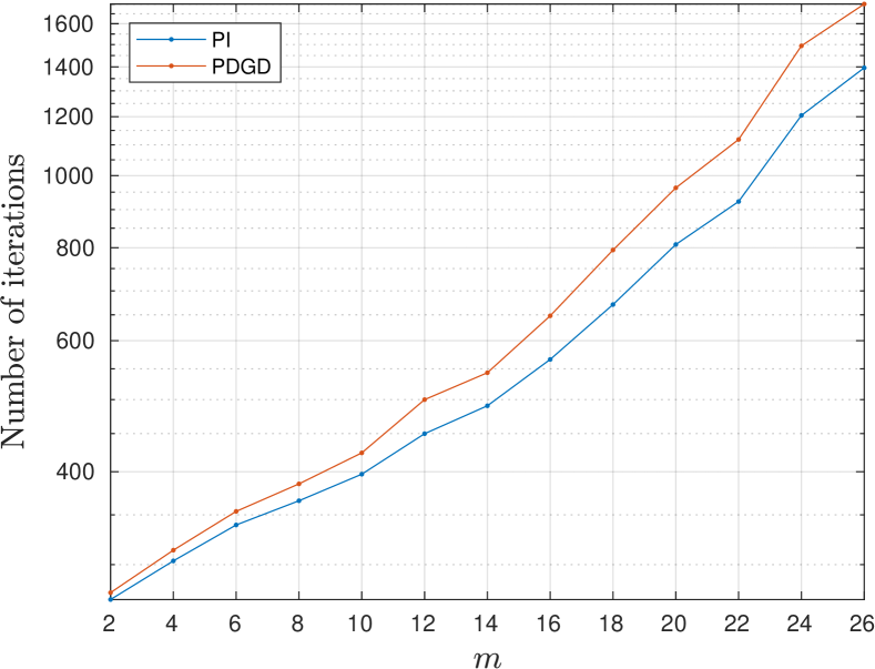
Figure 4: Number of iterations to converge for PI control and PDGD in a convex quadratic example, with $m$ constraints. The results are averaged over 400 random runs.

Fig. 4 shows the average number of iterations required to converge to the desired minimum against $m$. For all the considered values of $m$, PI requires fewer iterations on average than PDGD, as expected from the theoretical results in Section 3. In particular, the gain in the number of iterations tends to increase with $m$, and is larger than $15\%$ for $m\geq 18$.

5.2 Shidoku puzzle

Shidoku is a 4x4 version of the popular 9x9 Sudoku puzzle. Given an initial scheme, as reported in Fig. 5, the aim is to fill the empty cells with integers $x_{i,j}\in\{1,2,3,4\}$ such that each row, each column and each 2x2 corner block contain the integers $1,2,3,4$.

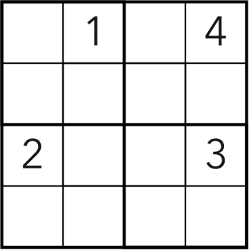
Figure 5: Shidoku puzzle to be solved.

We can formulate the game in terms of the solution of polynomial equations on the values $x_{i,j}$ of each cell $(i,j)$, $i,j=1,\dots,4$. First of all, $x_{i,j}\in\{1,2,3,4\}$ is guaranteed by $\prod_{h=1}^{4}(x_{i,j}-h)=0$. Then, we obtain no repetition in groups of 4 cells by imposing the product equal to $24$ and the sum equal to $10$. In summary, given the corner blocks

$$\begin{split}B_{1}&=\{(1,1),(1,2),(2,1),(2,2)\}\\ B_{2}&=\{(1,3),(1,4),(2,3),(2,4)\}\\ B_{3}&=\{(3,1),(3,2),(4,1),(4,2)\}\\ B_{4}&=\{(3,3),(3,4),(4,3),(4,4)\}.\end{split}$$

we have

$$\text{Columns: for }j=1,\dots,4,$$ (90)

$$~{}~{}~{}~{}\sum_{i=0}^{4}x_{ij}=10,\quad\prod_{i=0}^{4}x_{ij}=24.$$

$$\text{Rows: for }i=1,\dots,4,$$

$$~{}~{}~{}~{}\sum_{j=0}^{4}x_{ij}=10,\quad\prod_{j=0}^{4}x_{ij}=24.$$

$$\text{Blocks: for }k=1,\dots,4,$$

$$~{}~{}~{}~{}\sum_{(i,j)\in B_{k}}x_{ij}=10,\quad\prod_{(i,j)\in B_{k}}x_{ij}=24.$$

$$\text{Restriction to integers: for }i,j=1,\dots,4,$$

$$~{}~{}~{}~{}\prod_{h=1}^{4}(x_{ij}-h)=0.$$

Initial conditions as in Fig. 5:

$$~{}~{}~{}~{}x_{1,2}=1\quad x_{1,4}=4\quad x_{3,1}=2\quad x_{3,4}=3.$$

Equations (90) represent non-convex polynomial constraints. We can solve the corresponding optimization problem through the proposed feedback control framework if we associate them with any constant cost function. In particular, we use the PI control method to test its convergence and effectiveness in non-convex problems. We cannot apply the feedback linearization since we have $m=40$ equations in $n=12$ variables and $m>n$ is not consistent with Assumption 3.

As to the PI control method, we set $K_{i}=1,K_{p}=0.1$ and we generate random initial conditions according to $x_{i,j}(0)=|\xi_{i,j}|,\xi_{i,j}\sim\mathcal{N}(0,1)$, for each $i,j=1,\dots,4$ and $\lambda_{k}(0)\sim\mathcal{N}(0,1),k=1,\dots,m$, where $\mathcal{N}(0,\sigma)$ denotes the normal distribution with zero mean and variance $\sigma^{2}$. We integrate the ordinary differential equations that describe the closed-loop dynamics thanks to the MATLAB ode45 solver in the time interval $[0,100]$ seconds, corresponding to approximately $151700$ iterations.We perform 20 runs with different random initial conditions. The PI control method is always convergent in the given time interval.

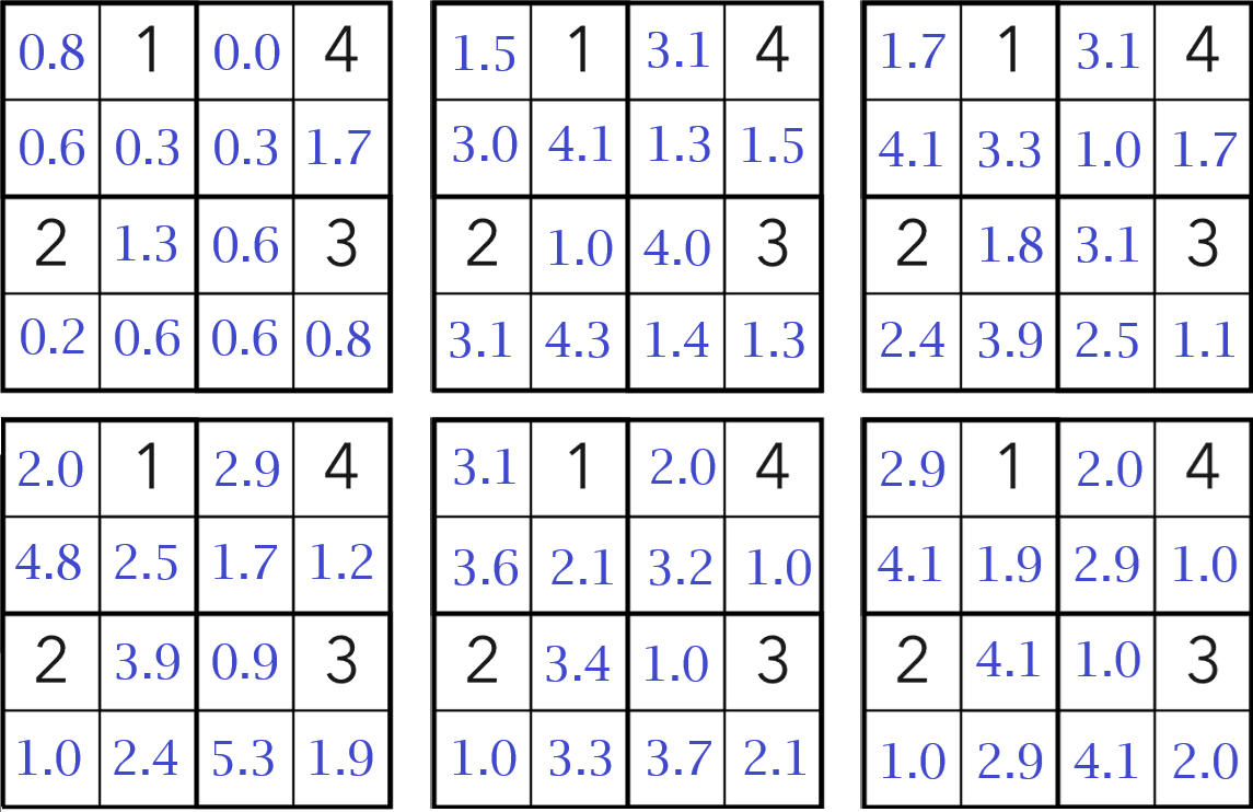
Figure 6: PI control method solves Shidoku puzzle. Evolution of the solution of the optimization variables at six equispaced sampling instants between initialization and convergence step $91027$, from top left to bottom right.

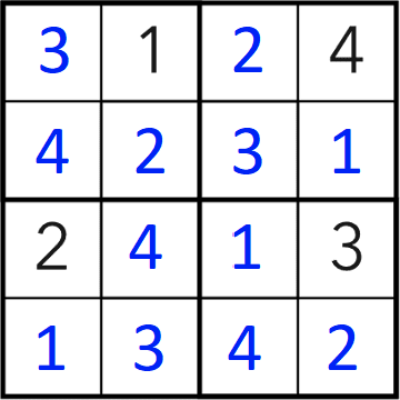
Figure 7: PI control method solves Shidoku puzzle: final correct solution.

We show an instance in Fig. 6, where we depict the evolution of the optimization variables for six equispaced sampling instants between the random initialization and the convergence to the correct solution at iteration 91027, shown in Fig. 7.

In conclusion, this test shows that the PI control method is convergent even in a non-convex problem that does not satisfy assumptions 1 and 2. For further investigation, we compare the PI control method to two state-of-the-art approaches for non-convex constrained optimization, interior-point method (IPM) and sequential quadratic programming, through the fmincon function in MATLAB. We perform 20 runs with random initial conditions for the two of them. We observe that IPM fails in all the runs due to numerical issues. More precisely, the linear system of KKT conditions to solve at each iteration is poorly conditioned, which affects the solution; see, e.g., [24, Chapter 19] for details. On the other hand, sequential quadratic programming converges to an infeasible point in all the runs.

5.3 Gray-box non-linear system identification

In this example, we consider the identification of the discrete-time nonlinear system described by the following regressor form

$$\begin{split}y(k)=&\theta_{1}e^{-(y(k-1))^{2}}+\theta_{2}(u(k-1))^{2}+\\ \qquad&\theta_{3}u(k-2)y(k-1)+\theta_{4}(u(k-2))^{\theta_{5}}\end{split}$$ (91)

using $N=400$ measurements of the input sequence $u(k)$ and noisy measurements of the output sequence $\tilde{y}(k)=y(k)+\zeta(k)$, where $\zeta(k)$ represents the noise.

Since the system is not affine in the parameters, we cannot employ standard solutions based on least-squares regression. We look for the parameter vector $\theta^{\star}\in\mathbb{R}^{5}$ that minimizes the $\ell_{2}$ norm, i.e., the noise sequence $\zeta(k)$ energy. This approach leads to the formulation of the following non-convex optimization problem:

$$\begin{split}[\theta^{\star},y^{\star}]&=\underset{\theta\in\mathbb{R}^{5},y\in\mathbb{R}^{N}}{\operatorname{arg}\,\operatorname{min}}\;\sum_{k=1}^{N}(y_{k}-\tilde{y}(k))^{2}\\ &\text{subject to:}\\ &-y_{k}+\theta_{1}e^{-y_{k-1}^{2}}+\theta_{2}(u(k-1))^{2}+\\ &\theta_{3}u(k-2)y_{k-1}+\theta_{4}(u(k-2))^{\theta_{5}}=0\\ &\qquad k=3,\dots,N.\end{split}$$ (92)

We solve problem (92) using the feedback linearization method developed in Section 4. We define the controller $\mathcal{G}$ in (64) according to (65) , with $K_{i}=1$ for each $i=1,\dots,m$.

We integrate the ordinary differential equations that describe the closed-loop dynamics in the time interval $t=[0,20]$ seconds by using Euler discretization with step size $10^{-2}$ seconds. We set normally distributed initial conditions.

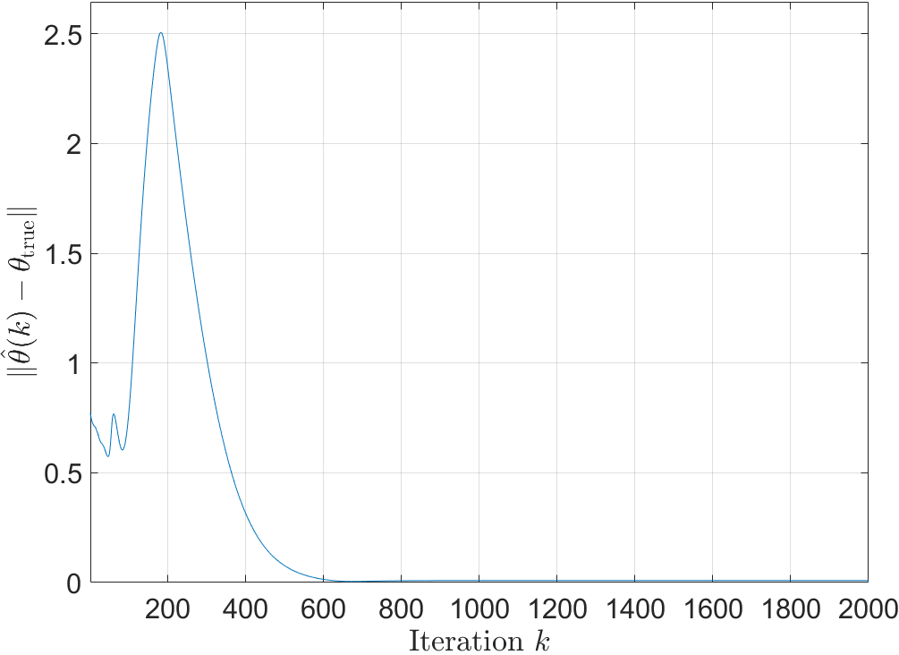
Figure 8: Gray-box non-linear system identification: evolution of the estimation error. We denote by $\hat{\theta}(k)$ the estimates obtained with the feedback linearization-based algorithm at iteration $k$, and by $\theta_{\rm true}$ the true parameter vector.

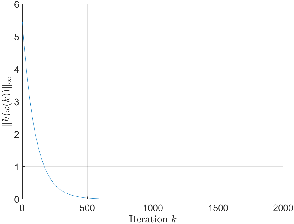
Figure 9: Gray-box non-linear system identification: evolution of the $\ell_{\infty}$-norm of the constraints function $h$. In the figure, $x(k)$ refers to the estimate, at iteration $k$, of $y$ and $\theta$ in (92).

Fig. 8 shows the $\ell_{2}$-norm of the estimation error as a function of the algorithm iteration. Fig. 9 shows the evolution of the $\ell_{\infty}$-norm of the constraints: as expected, it converges to zero.

For comparison, we solve problem (92) through IPM implemented with the fmincon MATLAB function and initialized with the same initial conditions used for the feedback linearization method. We use MATLAB R2021b on a processor i7-10700, 2.90GHz with 32 GB of DDR4 RAM.

Table 1: Gray-box non-linear system identification: comparison of parameter estimates for the proposed feedback linearization approach and IPM, denoted by $\hat{\theta}$ and $\theta_{\rm IPM}$, respectively.

$\theta_{\rm true}$	$\hat{\theta}$	$\theta_{\rm IPM}$
$0.5$	$0.496$	$0.489$
$-0.3$	$-0.300$	$-0.300$
$-0.7$	$-0.699$	$-0.695$
$-0.35$	$-0.345$	$-0.338$
$0.8$	$0.815$	$0.804$

Table 1 compares the estimated parameters. We observe that both feedback linearization and IPM provide accurate estimates, the respective errors being $\|\theta_{\rm true}-\hat{\theta}\|_{2}=0.0163$ and $\|\theta_{\rm true}-\theta_{\rm IPM}\|_{2}=0.0175$.

Let us analyze the computational complexity. The time required by the proposed feedback linearization approach is $9.8$ seconds, while IPM requires $64.4$ seconds. Moreover, the proposed feedback linearization method is less memory expensive with respect to IPM, as expected when we compare first-order and second-order methods, because it requires storing only the Jacobian of the constraints and not the Hessian matrix. More precisely, given $m\leq n$, the feedback linearization approach requires $n+nm+\frac{1}{2}m^{2}+m$ floating point numbers, while IPM requires $n+n^{2}+nm+3m$ floating point numbers. In both cases, we assess this number by assuming to store only the triangular part of the symmetric matrices. Concerning IPM, the leading term $n^{2}$ is due to the sum of $m+1$ Hessian matrices, one for $f(x)$ and $m$ for $h_{i}(x)$, of dimension $n\times n$. Thus, we need $\frac{1}{2}n^{2}$ variables to compute the current Hessian and a further $\frac{1}{2}n^{2}$ ones are used to store the partial sum.

In conclusion, there is a gain of $2m+n^{2}-\frac{1}{2}m^{2}$ floating-point numbers by using the proposed feedback linearization method instead of IPM.

Moreover, each iteration in feedback linearization requires $O(m^{3})$ floating-point operations (FLOPs) to invert the matrix $J_{h}J_{h}^{\top}\in{}^{m\times m}$, while each iteration of IPM requires $O((n+m)^{3})$ FLOPs to solve a linear system of dimension $n+m$.

We notice that similar considerations apply to sequential quadratic programming, which needs approximately the same memory and computations as IPM; see, e.g., [24, Chapter 18].

5.4 Industrial chemical process problem

We consider a problem that arises in the context of industrial chemical processes: the propane, isobutane, and n-butane nonsharp separation presented in [1]. It is about a three-component feed mixture required to separate products into two three-component products. This problem is included in the benchmark suite of real-world, non-convex problems proposed in [18] to test optimization algorithms. The mathematical formulation of the problem, reported in [18, Sec. 2.1.5], is as follows. Given $x=(x_{1},\dots,x_{48})$, minimize $f(x)$ defined as

$$\begin{split}f(x)&=c_{11}+\left(c_{21}+c_{31}x_{24}+c_{41}x_{28}+c_{51}x_{33}+c_{61}x_{34}\right)x_{5}\\ &+c_{12}+\left(c_{22}+c_{32}x_{26}+c_{42}x_{31}+c_{52}x_{38}+c_{62}x_{39}\right)x_{13}\end{split}$$

where $c_{11}=0.23947$, $c_{12}=0.75835$, $c_{21}=-0.0139904$, $c_{22}=-0.0661588$, $c_{31}=0.0093514$, $c_{32}=0.0338147$, $c_{41}=0.0077308$, $c_{42}=0.0373349$, $c_{51}=-0.0005719$, $c_{52}=0.0016371$, $c_{61}=0.0042656$, $c_{62}=0.0288996$, subject to

$$h_{1}({x})=x_{4}+x_{3}+x_{2}+x_{1}=300,$$

$$h_{2}({x})=x_{6}-x_{8}-x_{7}=0,$$

$$h_{3}({x})=x_{9}-x_{12}-x_{10}-x_{11}=0,$$

$$h_{4}({x})=x_{14}-x_{17}-x_{15}-x_{16}=0,$$

$$h_{5}({x})=x_{18}-x_{20}-x_{19}=0,$$

$$h_{6}({x})=x_{6}x_{21}-x_{24}x_{25}=0,$$

$$h_{7}({x})=x_{14}x_{22}-x_{26}x_{27}=0,$$

$$h_{8}({x})=x_{9}x_{23}-x_{28}x_{29}=0$$

$$h_{9}({x})=x_{18}x_{30}-x_{31}x_{32}=0,$$

$$h_{10}({x})=x_{25}-x_{5}x_{33}=0,$$

$$h_{11}({x})=x_{29}-x_{5}x_{34}=0,$$

$$h_{12}({x})=x_{35}-x_{5}x_{36}=0,$$

$$h_{13}({x})=x_{37}-x_{13}x_{38}=0,$$

$$h_{14}({x})=x_{27}-x_{13}x_{39}=0$$

$$h_{15}({x})=x_{32}-x_{13}x_{40}=0$$

$$h_{16}({x})=x_{25}-x_{6}x_{21}-x_{9}x_{41}=0,$$

$$h_{17}({x})=x_{29}-x_{6}x_{42}-x_{9}x_{23}=0,$$

$$h_{18}({x})=x_{35}-x_{6}x_{43}-x_{9}x_{44}=0,$$

$$h_{19}({x})=x_{37}-x_{14}x_{45}-x_{18}x_{46}=0,$$

$$h_{20}({x})=x_{27}-x_{14}x_{22}-x_{18}x_{47}=0,$$

$$h_{21}({x})=x_{32}-x_{14}x_{48}-x_{18}x_{30}=0,$$

$$h_{22}({x})=0.33x_{1}+x_{15}x_{45}-x_{25}=0$$

$$h_{23}({x})=0.33x_{1}+x_{15}x_{22}-x_{29}=0$$

$$h_{24}({x})=0.33x_{1}+x_{15}x_{48}-x_{35}=0,$$

$$h_{25}({x})=0.33x_{2}+x_{10}x_{41}-x_{37}=0$$

$$h_{26}({x})=0.33x_{2}+x_{10}x_{23}-x_{27}=0$$

$$h_{27}({x})=0.33x_{2}+x_{10}x_{44}-x_{32}=0$$

$$h_{28}({x})=0.33x_{3}+x_{7}x_{21}+x_{11}x_{41}+x_{16}x_{45}+x_{19}x_{46}=30,$$

$$h_{29}({x})=0.33x_{3}+x_{7}x_{42}+x_{11}x_{23}+x_{16}x_{22}+x_{19}x_{47}=50,$$

$$h_{30}({x})=0.33x_{3}+x_{7}x_{43}+x_{11}x_{44}+x_{16}x_{48}+x_{19}x_{30}=30,$$

$$h_{31}({x})=x_{33}+x_{34}+x_{36}=1,$$

$$h_{32}({x})=x_{21}+x_{42}+x_{43}=1,$$

$$h_{33}({x})=x_{41}+x_{23}+x_{44}=1,$$

$$h_{34}({x})=x_{38}+x_{39}+x_{40}=1,$$

$$h_{35}({x})=x_{45}+x_{22}+x_{48}=1,$$

$$h_{36}({x})=x_{46}+x_{47}+x_{30}=1,$$

$$h_{37}({x})=x_{43}=0,$$

$$h_{38}({x})=x_{46}=0.$$

with bounds

$$0\leq x_{1},\ldots,x_{20}\leq 150,$$

$$0\leq x_{25},x_{27},x_{32},x_{35},x_{37},x_{29}\leq 30,$$

$$0\leq x_{21},x_{22},x_{23},x_{30},x_{33},x_{34},x_{36},x_{38},x_{39}\leq 1,$$

$$0\leq x_{40},x_{42},x_{43},x_{44},x_{45},x_{46},x_{47},x_{48}\leq 1,$$

$$0.85\leq x_{24},x_{26},x_{28},x_{31}\leq 1.$$

The problem consists of $n=48$ optimization variables, a bilinear cost function, and $m=38$ linear and bilinear equality constraints. The overall problem is non-convex. Moreover, there are $47$ constrained variables in bounded intervals, which give rise to $94$ inequality constraints. To deal with the inequality constraints, we reformulate them by using squared-slack variables, as discussed, e.g., in [3, Sec. 3.3.2]. The basic idea is that we can rewrite any inequality $g(x)\leq 0$ as $g(x)+z^{2}=0$, where $z\in\mathbb{R}$ is a slack variable.

For this problem, the benchmark objective value is $f(x)=2.1158$, as reported in [18, Table 3].

We perform the optimization through the feedback linearization method, implemented in MATLAB R2021b, on a processor i7-10700, 2.90GHz with 32 GB of DDR4 RAM. As in the previous example, we design the $\mathcal{G}$ controller, see (64), by pole placement. We place the closed-loop pole at $-10$. We integrate the closed-loop differential equations in the time interval $[0,3]$ seconds using Euler discretization with step size $5\cdot 10^{-5}$ seconds.

We randomly set the initial conditions with uniform distribution in $[0,50]$. We run the algorithm $50$ times with different realizations of the initial conditions. In all the runs, the algorithm converges to feasible solutions within a tolerance of $10^{-7}$ for each constraint. The achieved objective values are distributed according to the histogram in Fig. 10; the mean value is $2.332$, and the standard deviation is $0.1852$. Moreover, the best achieved objective value is $2.0333$, which improves the benchmark $2.1158$. In Fig. 10, we also report the distribution of the time required to converge; the mean value is $7.22$ seconds, and the standard deviation is $0.33$ seconds.

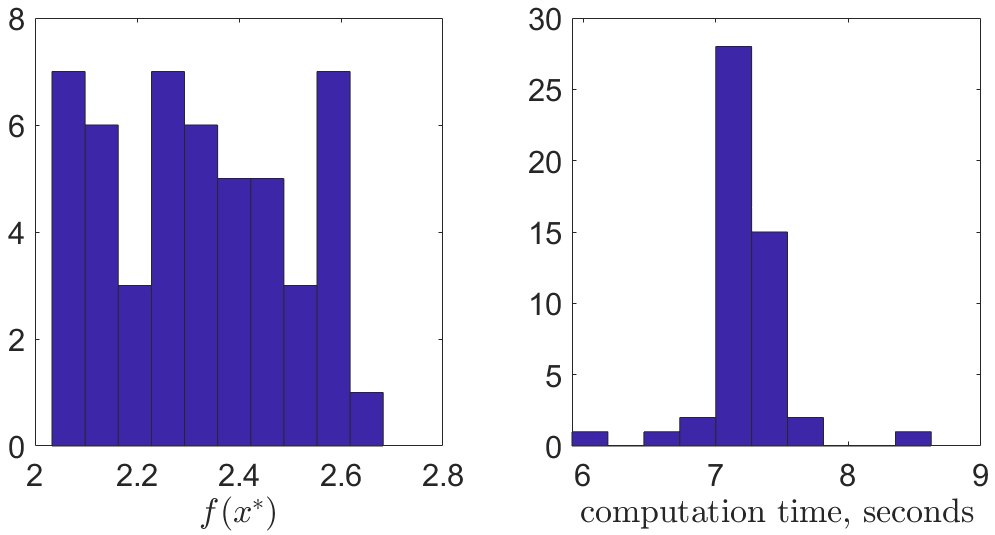
Figure 10: Industrial chemical process problem: distribution of the achieved objective values (left) and distribution of the required time to converge (right)

We finally remark that IPM is an alternative solver for this problem, but it suffers the increase of required memory to store the Hessian matrix; see the analysis of computational complexity in Section 5.3.

In conclusion, this experiment proves that the proposed feedback linearization approach is valuable in large-scale, non-convex optimization problems arising from real-world applications. Moreover, using squared-slack variables is a feasible approach to deal with inequality constraints in this example, even if it increases the number of optimization variables and introduces additional non-convex constraints.

6 Conclusion

This paper proposes a control-theoretic approach to develop novel algorithms for convex and non-convex, equality-constrained optimization. Based on the solution of the first-order necessary conditions, we show that the considered class of optimization problems is equivalent to a class of output regulation problems. The Lagrange multipliers of the problem are the control inputs of the dynamic system to regulate. We analyze two approaches to design their control: PI control and feedback linearization. Then, we propose a theoretical analysis of the convergence properties of the two of them. Our research rigorously proves the convergence of the PI control method in strongly convex problems and provides a comprehensive assessment of its convergence rate. Furthermore, we establish the local convergence of the feedback linearization method in non-convex problems, thereby reinforcing the robustness and reliability of our findings. Finally, we tested the two methods in experiments. This validation process confirms the theoretical results and sheds light on the practical effectiveness of the methods, particularly in comparison to the state-of-the-art optimization algorithms.

Future extensions of this work include the development of methods that envisage inequality constraints in a more effective way than the use of squared-slack variables and non-differentiable cost functions.

References

• [1] A. Aggarwal and C.A. Floudas. Synthesis of general distillation sequences-nonsharp separations. Comput. Chemical Eng., 14(6):631–653, 1990.
• [2] Kenneth Joseph Arrow, Leonid Hurwicz, and Hollis Burnley Chenery. Studies in linear and non-linear programming. Stanford University Press, 1958.
• [3] D.P. Bertsekas. Nonlinear Programming. Athena Scientific, Belmont, Massachusetts, 2nd edition, 1999.
• [4] Amit Bhaya and Eugenius Kaszkurewicz. A control-theoretic approach to the design of zero finding numerical methods. IEEE Trans. Autom. Control, 52(6):1014–1026, 2007.
• [5] S. Boyd, N. Parikh, E. Chu, B. Peleato, and J. Eckstein. Distributed optimization and statistical learning via the alternating direction method of multipliers. Found. Trends Mach. Learn., 3(1):1 – 122, 2010.
• [6] Christopher I. Byrnes and Alberto Isidori. A frequency domain philosophy for nonlinear systems, with applications to stabilization and to adaptive control. In IEEE Conf. Decis. Control (CDC), pages 1569–1573, 1984.
• [7] Zhehui Chen, Xingguo Li, Lin Yang, Jarvis Haupt, and Tuo Zhao. On constrained nonconvex stochastic optimization: A case study for generalized eigenvalue decomposition. In Proc. Int. Conf. Arti. Intell. Stat. (AISTATS), volume 89, pages 916–925, 2019.
• [8] Neil K. Dhingra, Sei Zhen Khong, and Mihailo R. Jovanović. The proximal augmented lagrangian method for nonsmooth composite optimization. IEEE Trans. Autom. Control, 64(7):2861–2868, 2019.
• [9] Dongsheng Ding and Mihailo R. Jovanović. Global exponential stability of primal-dual gradient flow dynamics based on the proximal augmented lagrangian. In Proc. Amer. Control Conf. (ACC), pages 3414–3419, 2019.
• [10] Omer Elkabetz and Nadav Cohen. Continuous vs. discrete optimization of deep neural networks. In Proc. Adv. Neural Infor. Process. Syst. (NeurIPS), volume 34, pages 4947–4960, 2021.
• [11] Guilherme França, Daniel P. Robinson, and René Vidal. ADMM and accelerated ADMM as continuous dynamical systems. In Proc. Int. Conf. Mach. Learn. (ICML), pages 1559–1567, 2018.
• [12] Ian Goodfellow, Yoshua Bengio, and Aaron Courville. Deep Learning. MIT Press, 2016.
• [13] Bin Hu and Laurent Lessard. Control interpretations for first-order optimization methods. In Amer. Control Conf. (ACC), pages 3114–3119, 2017.
• [14] Alberto Isidori. Nonlinear Control Systems. Springer London, 1995.
• [15] Alberto Isidori. The zero dynamics of a nonlinear system: From the origin to the latest progresses of a long successful story. Europ. J. Control, 19(5):369–378, 2013.
• [16] H. K. Khalil. Nonlinear Systems. Pearson Education. Prentice Hall, 3rd edition, 2002.
• [17] T. Kose. Solutions of saddle value problems by differential equations. Econometrica, 24(1):59–70, 1956.
• [18] Abhishek Kumar, Guohua Wu, Mostafa Z. Ali, Rammohan Mallipeddi, Ponnuthurai Nagaratnam Suganthan, and Swagatam Das. A test-suite of non-convex constrained optimization problems from the real-world and some baseline results. Swarm and Evolutionary Computation, 56:100693, 2020.
• [19] Laurent Lessard, Benjamin Recht, and Andrew Packard. Analysis and design of optimization algorithms via integral quadratic constraints. SIAM J. Optim., 26(1):57–95, 2016.
• [20] David G. Luenberger and Yinyu Ye. Linear and Nonlinear Programming. Springer Publishing Company, Inc., 4th edition, 2015.
• [21] Deyuan Meng. Feedback of control on mathematics: Bettering iterative methods by observer system design. IEEE Trans. Autom. Control, 68(4):2498–2505, 2023.
• [22] Deyuan Meng and Yuxin Wu. Control design for iterative methods in solving linear algebraic equations. IEEE Trans. Autom. Control, 67(10):5039–5054, 2022.
• [23] Michael Muehlebach and Michael Jordan. A dynamical systems perspective on nesterov acceleration. In Proc. Int. Conf. Mach. Learn. (ICML), pages 4656–4662. PMLR, 2019.
• [24] Jorge Nocedal and Stephen J. Wright. Numerical optimization. Springer, 2006.
• [25] Neal Parikh and Stephen Boyd. Proximal algorithms. Foundations and Trends in Optimization, 1(3):127–239, 2014.
• [26] Guannan Qu and Na Li. On the exponential stability of primal-dual gradient dynamics. IEEE Control Syst. Lett., 3(1):43–48, 2019.
• [27] A Saxe, J McClelland, and S Ganguli. Exact solutions to the nonlinear dynamics of learning in deep linear neural networks. In Proc. of the International Conference on Learning Represenatations 2014. International Conference on Learning Represenatations 2014, 2014.
• [28] Johannes Schropp and Ivan Singer. A dynamical systems approach to constrained minimization. Numer. Funct. Anal. Optim., 21:537–551, 2000.
• [29] Weijie Su, Stephen Boyd, and Emmanuel J. Candès. A differential equation for modeling Nesterov’s accelerated gradient method: Theory and insights. J. Mach. Learn. Res., 17(153):1–43, 2016.
• [30] Hiroshi Yamashita. A differential equation approach to nonlinear programming. Mathematical Programming, 18(1):155–168, 1980.
• [31] Limei Zhou, Yue Wu, Liwei Zhang, and Guang Zhang. Convergence analysis of a differential equation approach for solving nonlinear programming problems. Applied Mathematics and Computation, 184(2):789–797, 2007.