Tests for categorical data beyond Pearson: A distance covariance and energy distance approach

Abstract

Categorical variables are of uttermost importance in biomedical research. When two of them are considered, it is often the case that one wants to test whether or not they are statistically dependent. We show weaknesses of classical methods —such as Pearson’s and the $G$-test— and we propose testing strategies based on distances that lack those drawbacks. We first develop this theory for classical two-dimensional contingency tables, within the context of distance covariance, an association measure that characterises general statistical independence of two variables. We then apply the same fundamental ideas to one-dimensional tables, namely to the testing for goodness of fit to a discrete distribution, for which we resort to an analogous statistic called energy distance. We prove that our methodology has desirable theoretical properties, and we show how we can calibrate the null distribution of our test statistics without resorting to any resampling technique. We illustrate all this in simulations, as well as with some real data examples, demonstrating the adequate performance of our approach for biostatistical practice.

1 Introduction

In previous work by us (Castro-Prado et al., 2023), an interesting dataset from complex disease genomics motivated us to define distances on discrete spaces of cardinality 3 and test independence among variables whose support lie on such spaces. However, since the times of Karl Pearson (more than a century ago), the corresponding test for categorical variables with an arbitrary finite number of categories has been of paramount interest to manifold applications. As a matter of fact, independence of categorical variables ranks among the most often tested hypotheses in biomedical practice (Berrett and Samworth, 2021). Discrete data arise in health sciences in a variety of contexts (Agresti, 2019; Preisser and Koch, 1997) — for measuring responses to treatments, signposting the stage of a disease (or whether the disease is present), establishing subgroups after a diagnosis, and so forth.

In this paper, we present the distance and kernel counterpart (Edelmann and Goeman, 2022) perspective on what Pearson (1900) did. We derive some theory for independence testing and extend it to the problem of goodness of fit. We finally illustrate with synthetic and real data examples the performance of our methodology, including the comparison with competing methods.

For independence, we will consider categorical variables $X\in\{1,\ldots,I\}\}$ and $Y\in\{1,\ldots,J\}\}$. Given an IID sample $\{(X_{m},Y_{m})\}_{m=1}^{n}$, one can construct the $I\times J$ contingency table $(n_{ij})_{i,j}$ by counting the observations per pair of categories $(X,Y)$:

$$n_{ij}=\sum_{m=1}^{n}1_{\{X_{m}=i,Y_{i}=j\}}.$$

Under the null hypothesis, we expect to observe, in each cell:

$$n_{ij}^{*}:=\frac{1}{n}\sum_{j=1}^{n}n_{ij}\sum_{i=1}^{n}n_{ij}.$$

One of the most common test statistics is Pearson’s:

$$\chi^{2}=\sum_{i=1}^{I}\sum_{j=1}^{J}\frac{(n_{ij}-n^{*}_{ij})^{2}}{n^{*}_{ij}},$$

for which the $p$-values are either computed using a chi-squared distribution with $(I-1)(J-1)$ degrees of freedom, or using permutations. The same holds for the null distribution of the $G$-test (which is essentially the likelihood ratio test for this problem):

$$G=2\sum_{i=1}^{I}\sum_{j=1}^{J}n_{ij}\log\left(\frac{n_{ij}}{n^{*}_{ij}}\right).$$

Other available methods include Fisher’s exact test and the $U$-statistic permutation test (Berrett and Samworth, 2021). The authors of this last work very illustratively show how classical methods have important limitations related to imbalanced cell counts, which justifies the need for new techniques for such a relevant problem.

For the problem of goodness of fit, it is customary to resort to Pearson’s (chi-squared) test, for which the philosophy is, once more “the squared difference of the observed and the expected, divided by the expected;” now with the difference that the table is $1\times I$ and the expected cell counts will be

$$n\operatorname{P}_{H_{0}}\{X=i\}.$$

The scope of this work will be to address the testing for independence and goodness of fit with categorical data, using the aforementioned techniques, collectively known as energy statistics (Székely and Rizzo, 2017). The remainder of the article is organised as follows. Section 2 contains our novel approach to the testing for independence between two categorical variables. In Section 3, we develop the testing for goodness of fit to a discrete distribution using the same basic notions, but with different theoretical tools. Some illustrative simulations are reported in Section 4. In Section 5, we apply the method to real data, to show applicability. Concluding remarks are given in Section 6. Proves for our theoretical results are given in appendices A and B.

2 The distance covariance test of independence between two categorical variables

Given an IID sample $\{(X_{i},Y_{1})\}_{i=1}^{n}$ of $(X,Y)$, a consistent (but biased) estimator for the generalised distance covariance between our jointly distributed two random variables is given by

$$\widehat{V}=\widehat{T}_{1}-2\widehat{T}_{2}+\widehat{T}_{3},$$

where

$$\widehat{T}_{1} =\frac{1}{n^{2}}\sum_{i,j=1}^{n}d_{\mathcal{X}}(X_{i},X_{j})\,d_{\mathcal{Y}}(Y_{i},Y_{j}),$$

$$\widehat{T}_{2} =\frac{1}{n^{3}}\sum_{i=1}^{n}\big{(}\sum_{j=1}^{n}d_{\mathcal{X}}(X_{i},X_{j})\big{)}\,\big{(}\sum_{j=1}^{n}d_{\mathcal{Y}}(Y_{i},Y_{j})\big{)},$$

$$\widehat{T}_{3} =\frac{1}{n^{4}}\Big{(}\sum_{i,j=1}^{n}d_{\mathcal{X}}(X_{i},X_{j})\Big{)}\,\Big{(}\sum_{i,j=1}^{n}d_{\mathcal{Y}}(Y_{i},Y_{j})\Big{)}.$$

We assume that the supports $\mathcal{X}$ and $\mathcal{Y}$ of $X$ and $Y$ respectively are finite, with cardinality $I\in\mathbb{Z}^{+}$ and $J\in\mathbb{Z}^{+}$. When it comes to deciding which (pseudo)metrics $d_{\mathcal{X}}$ and $d_{\mathcal{Y}}$ to equip them with, the only restriction we have for distance covariance (Székely et al., 2007) and associated techniques to work out is that we need to be in a (pseudo)metric structure of strong negative type (Jakobsen, 2017; Sejdinovic et al., 2013). Now the question would be which of those feasible distances it is the most convenient to use. Since we are working with categorical data and we want to be as agnostic as possible in terms of the underlying relationships among categories, in the following we will restrict ourselves to the case in which the metric structure on both marginal spaces reflects this agnosticism. In other words, we will equip both $\mathcal{X}$ and $\mathcal{Y}$ with the discrete distance (which we will henceforward denote simply as $d$ for both spaces):

$$d(z,z^{\prime})=1-\delta_{z\,z^{\prime}}=\operatorname{I}\{z\neq z^{\prime}\}$$

where $\delta_{\cdot\,\cdot}$ denotes the Kronecker delta and $(z,z^{\prime})$ is either in $\mathcal{X}\times\mathcal{X}$ or in $\mathcal{Y}\times\mathcal{Y}$. Alternatively, we could obtain the same test statistic by identifying the $I$ categories of $X$ with an orthonormal basis of $\mathbb{R}^{I}$ and then using the Euclidean distance and classical distance covariance (Székely et al., 2007), instead of its extension to metric spaces (Jakobsen, 2017; Lyons, 2013).

We now construct the $I\times J$ contingency table for the sample $\{(X_{i},Y_{1})\}_{i=1}^{n}$ of $(X,Y)$. Its $(i,j)$-th cell will be denoted by $n_{ij}$:

$$n_{ij}=\sum_{m=1}^{n}1_{\{X_{m}=i,Y_{i}=j\}}.$$

We call the $n_{ij}$’s observed cell counts, whereas their expected counterparts are their expected values under the null hypothesis (i.e., independence of $X,Y$).

We now introduce the notation $n_{i\cdot}$ and $n_{\cdot j}$ for the row and column sums of the contingency table:

$$n_{i\cdot}:=\sum_{j=1}^{n}n_{ij}=\sum_{m=1}^{n}1_{\{X_{m}=i\}};$$

$$n_{\cdot j}:=\sum_{i=1}^{n}n_{ij}=\sum_{m=1}^{n}1_{\{Y_{m}=j\}}.$$

These allow us to define the expected cell counts (under independence):

$$n^{*}_{ij}=\frac{1}{n}n_{i\cdot}n_{\cdot j}$$

By performing some algebraic manipulations, one can see that our test statistic can compactly be written as:

$$\widehat{V}=\frac{1}{n^{2}}\sum_{i=1}^{I}\sum_{j=1}^{J}(n_{ij}-n^{*}_{ij})^{2}$$ (1)

On the other hand, Pearson’s (chi-squared) test for independence is based on the statistic

$$\chi^{2}=\sum_{i=1}^{I}\sum_{j=1}^{J}\frac{(n_{ij}-n^{*}_{ij})^{2}}{n^{*}_{ij}},$$

which only differs in a “normalising” denominator in each term of the sum.

We now state the following result on the null distribution of our test statistic (1). The proof can be found on Appendix A.

2.1

Let $(X_{1},\ldots,X_{n})$ and $(Y_{1},\ldots,Y_{n})$ be IID samples of jointly distributed random variables $(X,Y)\in\{1,2,\ldots,I\}\times\{1,2,\ldots,J\}$, with $q_{i}:=P(X=i)$ and $r_{j}:=P(Y=j)$.

Consider $\mathcal{X}$ and $\mathcal{Y}$ equipped with the discrete metric. Then the empirical distance covariance between the two random variables can be written as:

$$\widehat{\operatorname{dCov}}_{\text{discrete}}^{2}(X,Y)=\frac{1}{n^{2}}\sum_{i=1}^{I}\sum_{j=1}^{J}(n_{ij}-n^{*}_{ij})^{2}$$

In addition, whenever $X$ and $Y$ are independent, for $n\to\infty$,

$$n\,\widehat{\operatorname{dCov}}_{\text{discrete}}^{2}(X,Y)\stackrel{{\scriptstyle\mathcal{D}}}{{\longrightarrow}}\sum_{i=1}^{I-1}\sum_{j=1}^{J-1}\lambda_{i}\mu_{j}Z_{ij}^{2}$$

where $Z_{ij}^{2}$ are independent chi-squared variables with one degree of freedom each. $\lambda_{1},\ldots,\lambda_{I}$ are the eigenvalues of matrix $\mathbf{A}=(a_{ij})_{I\times I}$, whose entries are:

$$a_{ij}=q_{i}\delta_{ij}-q_{i}q_{j},$$

where $\delta_{ij}$ is the Kronecker delta. Similarly $\{\mu_{1},\ldots,\mu_{J}\}$ is the spectrum of $\mathbf{B}=(b_{ij})_{J\times J}$, with

$$b_{ij}=r_{i}\delta_{ij}-r_{i}r_{j}.$$

It should be noted that $\mathbf{A}$ and $\mathbf{B}$ are the covariance matrices of a multinomial distribution multiplied by a factor (actually, of a “multi-Bernoulli” distribution).

In practice, when it comes to using the distribution above, we will take the empirical estimators $\hat{q}_{i}$ and $\hat{r}_{j}$, then construct estimators of $\mathbf{A}$ and $\mathbf{B}$ from them, to finally use the products of their eigenvalues as the coefficients in the linear combination of IID $\chi^{2}_{1}$’s.

Hence, obtaining the $p$-values of our test boils down to evaluating the distribution function of weighted sums of chi-squared variables. The approximation of quadratic forms of Gaussian variables has been very well studied historically and it arises fairly often in statistical practice (Duchesne and Lafaye de Micheaux, 2010). The algorithm by Imhof (1961) is arguably one of the best known ones, but its speed can come at the price of precision (Goeman et al., 2011). We instead chose to resort to Farebrother (1984) for our approximations, in the implementation by Duchesne and Lafaye de Micheaux (2010).

3 The energy test for goodness of fit to a discrete distribution

Let us once again consider a categorical variable $X$ with support $\mathcal{X}$ of cardinality $I\in\mathbb{Z}^{+}$, which we will assume to be $\{1,\ldots,I\}$ without loss of generality. We observe a sample $X_{1},\ldots,X_{n}$ IID $X$ and we will use it to test for $X\sim F$ having been drawn from a certain distribution $F_{0}$:

$$H_{0}:F=F_{0}$$

The distance-based statistic for this kind of test would be the adaptation of the one by Székely and Rizzo (2005) to our setting. Let $d$ denote once more the discrete distance on the support of $X$. Then, the energy distance between the sampling distribution and $F_{0}$ is:

$$\mathcal{E}_{n}=n\left[\frac{2}{n}\sum_{l=1}^{n}\operatorname{E}d(x_{l},X)-\operatorname{E}d(X,X^{\prime})-\frac{1}{n^{2}}\sum_{l,m=1}^{n}d(x_{l},x_{m})\right];$$

where $\{x_{l}\}_{l=1}^{n}$ is a sample realisation of $\{X_{l}\}_{l=1}^{n}$ and $X^{\prime}$ is an IID copy of $X$.

If we now define $p_{i}:=\operatorname{P}_{H_{0}}\{X=i\}$ (for $i=1,\ldots,I$), we have that the expected cell count for each category is $n_{i}^{*}:=np_{i}$, where as the observed cell count is simply:

$$n_{i}:=\sum_{l=1}^{n}\operatorname{I}\{X_{l}=i\}.$$

With this notation, and after some algebra, we can write our test statistic as:

$$\mathcal{E}_{n}=\frac{1}{n}\sum_{i=1}^{I}(n_{i}-n_{i}^{*})^{2},$$

which again resembles to Pearson’s without its denominator. As of its null distribution, we present the following result.

3.1

Let $(X_{1},\ldots,X_{n})$ be an IID sample of random variable $X\in\mathcal{X}=\{1,2,\ldots,I\}$.

Consider $\mathcal{X}$ equipped with the discrete metric. Then the energy distance test statistic for goodness of fit to a fixed distribution $\mathbf{p}=(p_{i})_{i=1}^{I}$ on $\{1,\ldots,I\}$ is:

$$\mathcal{E}_{n}=\frac{1}{n}\sum_{i=1}^{I}(n_{i}-n_{i}^{*})^{2},$$

with the observed counts being $n_{i}:=\sum_{l=1}^{n}\operatorname{I}\{X_{l}=i\}$ and the expected ones: $n_{i}^{*}=np_{i}$.

Then, whenever $X$ is distributed according to $\mathbf{p}$, for $n\to\infty$,

$$\mathcal{E}_{n}\stackrel{{\scriptstyle\mathcal{D}}}{{\longrightarrow}}\sum_{i=1}^{I-1}\lambda_{i}Z_{i}^{2}$$

where $Z_{i}^{2}$ are independent chi-squared variables with one degree of freedom each. $\lambda_{1},\ldots,\lambda_{I}$ are the eigenvalues of matrix $\mathbf{C}=(c_{ij})_{I\times I}$ with

$$c_{ij}=p_{i}\delta_{ij}-p_{i}p_{j},$$

where $\delta_{ij}$ is the Kronecker delta.

Note that, matrix $\mathbf{C}$ here is, once again, a covariance matrix of a multinomial, and therefore has zero as one of its eigenvalues and $I-1$ as its rank.

For the proof of the preceding theorem, we forward the reader to Appendix B.

4 Simulation study

As previously mentioned, the test statistic we present in Section 2 is (almost) the same as the USP test statistic by Berrett and Samworth (2021), with the fundamental difference being that theirs is the $U$-statistic counterpart of our $V$-statistic. The approach for the testing, however, is completely different, since they use permutations, whereas we derive the (asymptotic) null distribution of the test statistic (Theorem 2.1). We will therefore use the family of models for contingency tables with exponentially decaying marginals described by Berrett and Samworth (2021), as it provides a good framework for both assessing the calibration of significance and the performance in terms of power. We will compare our method with theirs, as well as with Pearson’s chi-squared test, Pearson’s test with permutations, Fisher’s exact test and the $G$-test.

Let us first define the model. For given $I$ and $J$, we define the cell probabilities of our contingency table under independence as:

$$p_{ij}^{(0)}:=\frac{2^{-(i+j)}}{(1-2^{-I})(1-2^{-J})}\text{; for }i=1,\ldots,I;j=1,\ldots,J.$$

The above expression is clearly the product of the marginal probabilities. It is also easy to see that the probability mass is maximised in the top-left corner of the contingency table and it decreases rightwards and downwards.

Now, for each $\varepsilon\in\mathbb{R}^{+}$ small enough so that no probabilities are out of $[0,2]$, we define $p_{ij}^{(\varepsilon)}$ as the following perturbation of $p_{ij}^{(0)}$:

$$p_{ij}^{(\varepsilon)}:=\begin{cases}p_{ij}^{(0)}+\varepsilon&\text{if }(i,j)\in\{(1,1),(2,2)\}\\ p_{ij}^{(0)}-\varepsilon&\text{if }(i,j)\in\{(1,2),(2,1)\}\\ p_{ij}^{(0)}&\text{otherwise }\end{cases};$$

where $\varepsilon\leq\min\left\{{\left[8(1-2^{-I})(1-2^{-J})\right]^{-1},1-\left[4(1-2^{-I})(1-2^{-J})\right]^{-1}}\right\}\approx 0.1295$. The larger $\varepsilon$ is (within its range), the further the contingency table is from the null hypothesis.

To follow exactly the footprints of Berrett and Samworth (2021), we consider $M=10^{4}$ replicates of contingency with $I=4$ rows and $J=8$ columns, containing $n=100$ observations. For each of the methods based on permutations, we chose $B=999$ as the number of resamples and we use the algorithm by Patefield (1981) to uniformly draw the contingency tables with given marginals.

For $\varepsilon=0$ we can see how we calibrate significance. Figure 1 shows the results with our method for some reference values and allows for a comparison with the ones for competing techniques. We see that we control type I error very satisfactorily, both when considering our results only and when comparing them with Pearson’s test with permutations, the USP and Fisher’s exact test. All the aforementioned tests perform satisfactorily in terms of calibration of $\alpha$. The $G$-test, however, proves to be far too conservative. Pearson’s chi-squared fails, too, when it comes to controlling the type I error, but does so in a less dramatic fashion (and it actually produces a good result for nominal $\alpha$ of 0.05). To find an explanation to this phenomenon, one should note that the model we are using features very small expected cell counts, which will tend to break down the heuristic rules as to when to use the chi-squared distribution with $(I-1)(J-1)$ degrees of freedom to compute $p$-values or not.

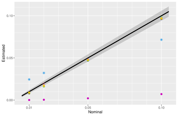
Figure 1: Nominal significance level ($\alpha$) versus empirical power under the null hypothesis ($\hat{\alpha}$), for the decaying marginals model, comparing our distance covariance method (golden points), Pearson’s chi-squared test (pale blue), Pearson’s test with permutations (dark red), the USP (black), Fisher’s exact test (green) and the $G$-test (purple). The grey shadow is a 95 % confidence band for $\hat{\alpha}$ given $\alpha$.

In terms of power, Figure 2 shows that we perform very similarly to the USP (which shows how our derivation of the null distribution is correct and that the asymptotic approximation is not very far off when $n=100$). The power curve of Fisher’s exact test is clearly under ours, whereas the one for the remaining classical methods is quite low for most values of $\varepsilon$.

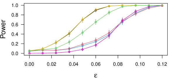
Figure 2: Power curve comparison for the decaying marginals model, comparing our distance covariance method (golden curve), Pearson’s chi-squared test (pale blue), Pearson’s test with permutations (dark red), the USP (black), Fisher’s exact test (green) and the $G$-test (purple). The $5\times 8$ cells of each contingency table were filled with $n=100$ observations. $M=10^{4}$ replicates were considered. Error bars span from $-3$ to $+3$ standard deviations for each value of parameter $\varepsilon$, which indicates the distance from the null hypothesis.

Other than the theoretical insight that using distance covariance provides (i.e., characterising general independence, the relationship to kernels and global tests, and so forth), we provide a relevant practical improvement with respect to the USP: running time. Our experiments show that we are around $2000$ times faster in testing than the USP.

5 Real data analyses

We begin by showing with a real biomedical example how our method can be used in practice. We consider data from Facal et al. (2022), where we observe $n=427$ patients of schizophrenia. For each of them, we consider a categorical variable $X$ indicating how chronic the psychiatric disorder is in that person (an index with four possible values, based on the admission history in health facilities), and another categorical variable $Y$ which indicates the PRS tercile (i.e., whether the polygenic risk score for schizophrenia of the patient is low, medium or high).

Although the clinical utility of PRSs is very limited at the individual level, they may be useful for the identification of specific quantiles of risk for stratification of a population to apply specific interventions (Torkamani et al., 2018). This is why it makes the most sense to consider PRS as a categorical variable (and not one with many categories) instead of working with its raw individual scores. The data for our example can be seen in Table 1.

Table 1: Contingency table for the chronicity dataset.

Chr. \ PRS	$\mathrm{T}_{1}$	$\mathrm{T}_{2}$	$\mathrm{T}_{3}$
Low	$12$	$9$	$4$	$25$
Middle-Low	$37$	$20$	$29$	$86$
Middle-high	$40$	$58$	$44$	$142$
High	$53$	$55$	$66$	$174$
	$142$	$142$	$143$	$427$

We can now apply the different methods of Section 4 to our dataset. Pearson’s test offers similar results with and without permutations, due to the lack of low (expected) cell counts. In both cases, the $p$-value is around 0.025 and one would reject independence for a nominal $\alpha$ of 0.05. The $G$-test offers a $p$ of 0.022, in line with Pearson’s. Fisher’s exact test also does not diverge much, with 0.024. Finally, the USP and the distance covariance yield $p$-values of 0.047 and 0.044. All things considered, in this case there one would tend to reject the null hypothesis of independence (when $\alpha=0.05$), which is consistent with the hypothesis that the PRS can measure how “sick” a patient is (or, more generally, how intense the trait of interest is).

6 Discussion and Conclusion

We have proposed a new test for the independence of categorical variables (one of the most often tested hypotheses in biomedical research) by using distance covariance, an association measure that characterises general statistical independence. As we allow for arbitrary dimensions of the contingency table, this extends the possibilities we showed on previous work (Castro-Prado et al., 2023) for the $3\times 3$ case. We have as well developed a novel testing strategy for the goodness of fit to a discrete distribution. For both methods, we demonstrate good performance and applicability, with simulations and analyses of relevant biomedical examples.

The test statistic we derive for independence happens to have a simple algebraic expression similar in spirit to that of Pearson’s $\chi^{2}$ test. We are not the first to see the connection between the two tests, as it was already mentioned in Remark 3.12 of Lyons (2013) and explored in some detail in the final section of Edelmann and Goeman (2022). Nevertheless, the proves we provide are original and we are the first ones (to our knowledge) to analyse the matter in detail. On top of that, we are not aware of any previous instance in the literature where a test for goodness of fit to a discrete distribution is built based on energy statistics.

Another test for independence that is related to ours is the one in Berrett and Samworth (2021). The main conceptual difference in our approaches is that we derive the asymptotic null distribution of our $V$-statistic and are able to satisfactorily use it in practice, whereas their testing is based on permutations (of a $U$-statistic). It is also noteworthy that, in that article, no mention is made of distance–based association measures, a relationship that we thoroughly explore. In return, we obtain from their results the conclusion that our test statistic is very close to being the minimum-variance unbiased estimator of the population USP-divergence statistic. As they indicate, if one assumes that the population quantity is meaningful (and we now know it is, given its connection to distance covariance), then the test statistic is a very good estimator of it.

A remarkable pragmatical difference between our goodness-of-fit test and the one for independence is that the latter does not require to plug in any frequencies to then estimate the multinomial covariance matrix and get the coefficients of the linear combination of chi-squared’s. In this case, the $p_{i}$’s are fixed and know, since they are given by the null hypothesis. However, when testing whether or not the population distribution belongs to a certain family of distributions, one would need to plug in the parameters in which the family is indexed.

All things considered, we have presented new methodology for to address important problems of practitioners, proven solid theoretical properties, explored connections with well-known methods, and illustrated all of it in simulated and real datasets. Future and current lines of work include extending these techniques to the study of associations between categorical and continuous data (Edelmann et al., 2024+).

Appendix A: Proof of theorem 2.1

We will firstly show that the distance covariance test statistic has the compact form similar to Pearson’s that we stated in the main manuscript, to then prove the asymptotic null distribution.

We will investigate the terms $\widehat{T}_{1},\widehat{T}_{2},\widehat{T}_{3}$ one by one, to then see how $\widehat{V}$ can be written as a simple expression.

$$\widehat{T}_{1} =\frac{1}{n^{2}}\sum_{i,j=1}^{n}d(X_{i},X_{j})\,d(Y_{i},Y_{j})$$

$$=\frac{1}{n^{2}}\sum_{i,j=1}^{n}1_{\{X_{i}\neq X_{j},Y_{i}\neq Y_{j}\}}$$

$$=\frac{1}{n^{2}}\sum_{i,j=1}^{n}1-1_{{\{X_{i}=X_{j}}}-1_{{\{Y_{i}=Y_{j}}}+1_{\{X_{i}=X_{j},Y_{i}=Y_{j}\}}$$

$$=1-\frac{1}{n^{2}}\sum_{k=1}^{m}n_{k\cdot}^{2}-\frac{1}{n^{2}}\sum_{l=1}^{r}n_{\cdot l}^{2}+\frac{1}{n^{2}}\sum_{k=1}^{m}\sum_{l=1}^{r}n_{kl}^{2}.$$

For $\widehat{T}_{2}$, we first observe that

$$\sum_{j=1}^{n}d(X_{i},X_{j})=n-n_{X_{i}\cdot},$$

and hence

$$\widehat{T}_{2} =\frac{1}{n^{3}}\sum_{k,l=1}^{n}(n-n_{k\cdot})(n-n_{\cdot l})n_{kl}$$

$$=1-\frac{1}{n^{2}}\sum_{k=1}^{m}n_{k\cdot}^{2}-\frac{1}{n^{2}}\sum_{l=1}^{r}n_{\cdot l}^{2}+\frac{1}{n^{3}}\sum_{k=1}^{m}\sum_{l=1}^{r}n_{k\cdot}n_{\cdot l}n_{kl}.$$

Finally

$$\sum_{i,j=1}^{n}d(X_{i},X_{j})=n^{2}-\sum_{k=1}^{m}n_{k\cdot}^{2}$$

and hence

$$\widehat{T}_{3} =\frac{1}{n^{4}}(n^{2}-\sum_{k=1}^{m}n_{k\cdot}^{2})(n^{2}-\sum_{l=1}^{r}n_{\cdot l}^{2})$$

$$=1-\frac{1}{n^{2}}\sum_{k=1}^{m}n_{k\cdot}^{2}-\frac{1}{n^{2}}\sum_{l=1}^{r}n_{\cdot l}^{2}+\frac{1}{n^{4}}\sum_{k=1}^{m}\sum_{l=1}^{r}n_{k\cdot}^{2}n_{\cdot l}^{2}.$$

When adding up the terms to obtain $\widehat{V}$, the terms $1$, $\frac{1}{n^{2}}\sum_{k=1}^{m}n_{k\cdot}^{2}$, $\frac{1}{n^{2}}\sum_{l=1}^{r}n_{\cdot l}^{2}$ cancel out and we obtain

$$\widehat{V} =\frac{1}{n^{2}}\sum_{k=1}^{m}\sum_{l=1}^{r}n_{kl}^{2}-\frac{2}{n^{3}}\sum_{k=1}^{m}\sum_{l=1}^{r}n_{k\cdot}n_{\cdot l}n_{kl}+\frac{1}{n^{4}}\sum_{k=1}^{m}\sum_{l=1}^{r}n_{k\cdot}^{2}n_{\cdot l}^{2}$$

$$=\frac{1}{n^{2}}\sum_{k=1}^{m}\sum_{l=1}^{r}(n_{kl}-\frac{1}{n}n_{k\cdot}n_{\cdot l})^{2}$$

$$=\frac{1}{n^{2}}\sum_{k=1}^{m}\sum_{l=1}^{r}(n_{kl}-n^{*}_{kl})^{2},$$

which is what we wanted to achieve.

Now, to start the way towards the asymptotic null distribution, let $\mathcal{Z}$ be either $\{1,\ldots,I\}$ or $\{1,\ldots,J\}$. Then the discrete metric

$$d(z,z^{\prime})=1-\delta_{zz^{\prime}},$$

is dual to the following kernel in the sense of Sejdinovic et al. (2013):

$$k(z,z^{\prime})=\delta_{zz^{\prime}},$$

which is known as the discrete kernel. Then clearly one can take the dummy function on each of $\mathcal{X}$ and $\mathcal{Y}$ as a feature map of the corresponding kernel/distance. We will denote them by $\phi:\mathcal{X}\longrightarrow\mathbb{R}^{I}$ and $\psi:\mathcal{Y}\longrightarrow\mathbb{R}^{J}$, where:

$$\phi_{i}(X)=1_{\{X=i\}},\quad\psi_{j}(Y)=1_{\{Y=j\}}.$$

Now we define the construct matrices $\mathbf{U}=(U_{ij})_{n\times I}$ and $\mathbf{V}=(V_{ij})_{n\times J}$ by transforming the $X$ and $Y$ samples with the feature maps:

$$U_{ki}=\phi_{i}(X_{k})\quad V_{kj}=\psi_{j}(Y_{k}).$$

Note that each of row of the previous matrices contains an observation of $\phi(X)\sim\operatorname{Multi-Bernoulli}(\mathbf{q})$ or $\psi(Y)\sim\operatorname{Multi-Bernoulli}(\mathbf{r})$ (respectively). Therefore:

$$\mathbf{1}^{\text{t}}\mathbf{U}\sim\operatorname{Multinomial}_{I}(n,\mathbf{q})$$

$$\mathbf{1}^{\text{t}}\mathbf{V}\sim\operatorname{Multinomial}_{J}(n,\mathbf{r})$$

Now, applying Equation 3 in Edelmann and Goeman (2022) to our feature maps, we get:

$$n\,\widehat{\operatorname{dCov}}_{\text{discrete}}^{2}(X,Y)=\frac{1}{n}\sum_{i=1}^{I}\sum_{j=1}^{J}[\mathbf{U}^{\text{t}}(\mathbf{I}_{n}-\mathbf{H})\mathbf{V}]^{2}_{i}j,$$

where $\mathbf{I}_{n}$ is the $n\times n$ identity matrix and $\mathbf{H}=\frac{1}{n}\mathbf{1}\mathbf{1}^{\text{t}}$ has constant entries equal to $\frac{1}{n}$. If we now define $\mathbf{C}\equiv(C_{ij})_{I\times J}:=\frac{1}{\sqrt{n}}\mathbf{U}^{\text{t}}(\mathbf{I}_{n}-\mathbf{H})\mathbf{V}$, we can compactly write our test statistic as a trace:

$$n\,\widehat{\operatorname{dCov}}_{\text{discrete}}^{2}(X,Y)=\operatorname{tr}[\mathbf{C}\mathbf{C}^{\text{t}}]=\operatorname{tr}[\mathbf{C}^{\text{t}}\mathbf{C}]=\sum_{i=1}^{I}\sum_{j=1}^{J}C_{ij}^{2}.$$

Expressing an empirical distance covariance as a trace of a matrix product, as we did above, is not unusual (Székely and Rizzo, 2017) and indeed it is a very computationally efficient way of evaluating it. Nonetheless, for continuing the proof we are going to write:

$$n\,\widehat{\operatorname{dCov}}_{\text{discrete}}^{2}(X,Y)=\mathbf{c}^{\text{t}}\mathbf{c};$$

where $\mathbf{c}:=\operatorname{vec}(\mathbf{C})\in\mathbb{R}^{IJ}$ is the vectorisation of matrix $\mathbf{C}$ (i.e., its image by the linear isomorphism $\mathbb{R}^{I\times J}\cong\mathbb{R}^{IJ}$).

If one adds a vector with constant components $\mathbf{a}=a\mathbf{1}$ to a column or row of a matrix, the result of centring it with matrix $\mathbf{I}-\mathbf{H}$ will be the same. Therefore, we can expand $\mathbf{C}$ as:

$$\mathbf{C}=\frac{1}{\sqrt{n}}(\mathbf{U}^{\text{t}}-\mathbf{q}\mathbf{1}^{\text{t}})(\mathbf{I}-\mathbf{H})(\mathbf{V}-\mathbf{1}\mathbf{r}^{\text{t}})=$$

$$=\frac{1}{\sqrt{n}}(\mathbf{U}^{\text{t}}-\mathbf{q}\mathbf{1}^{\text{t}})(\mathbf{V}-\mathbf{1}\mathbf{r}^{\text{t}})-\frac{1}{n^{3/2}}(\mathbf{U}^{\text{t}}-\mathbf{q}\mathbf{1}^{\text{t}})\mathbf{1}\mathbf{1}^{\text{t}}(\mathbf{V}-\mathbf{1}\mathbf{r}^{\text{t}}).$$

The second term of the previous sum is:

$$\mathbf{D}:=\frac{1}{\sqrt{n}}\>\left[\frac{1}{\sqrt{n}}\begin{pmatrix}\sum_{m=1}^{n}\left(\phi_{1}(X_{m})-q_{1}\right)\\ \ldots\\ \sum_{m=1}^{n}\left(\phi_{I}(X_{m})-q_{I}\right)\end{pmatrix}\right]\>\left[\frac{1}{\sqrt{n}}\left(\sum_{m=1}^{n}\left(\psi_{1}(Y_{m})-r_{1}\right),\ldots,\sum_{m=1}^{n}\left(\psi_{J}(Y_{m})-q_{J}\right)\right)\right]$$

By the central limit theorem, it is easy to see that each entry $D_{ij}$ of $\mathbf{D}$ converges in probability to zero, owing to the fact that:

$$\frac{1}{\sqrt{n}}\sum_{m=1}^{n}\left(\phi(X_{m})-\mathbf{q}\right)\stackrel{{\scriptstyle\mathcal{D}}}{{\longrightarrow}}\operatorname{\mathcal{N}}_{I}(\mathbf{0},\mathbf{A})$$

$$\frac{1}{\sqrt{n}}\sum_{m=1}^{n}\left(\psi(Y_{m})-\mathbf{r}\right)\stackrel{{\scriptstyle\mathcal{D}}}{{\longrightarrow}}\operatorname{\mathcal{N}}_{J}(\mathbf{0},\mathbf{B}).$$

Hence, $\operatorname{vec}(\mathbf{D})$ converges in probability to the $IJ-$dimensional null vector, and the limit in distribution of $c$ will be that of the vectorisation of:

$$\mathbf{E}:=\frac{1}{\sqrt{n}}(\mathbf{U}^{\text{t}}-\mathbf{q}\mathbf{1}^{\text{t}})(\mathbf{V}-\mathbf{1}\mathbf{r}^{\text{t}}).$$

We can write the $(i,j)$th entry of the previous matrix as: $E_{ij}=\frac{1}{\sqrt{n}}\sum_{m=1}^{n}G_{mij}$, where

$$G_{mij}=\left(\phi_{i}(X_{m})-q_{i}\right)\left(\psi_{j}(Y_{m})-r_{j}\right).$$

Now, we see that we can apply the CLT to

$$\operatorname{vec}(\mathbf{E})=\sum_{m=1}^{n}\operatorname{vec}(\mathbf{G}_{m}).$$

For a fixed $m\in\{1,\ldots,n\}$, let us see how the first and second moments of $\operatorname{vec}(\mathbf{G})\equiv\operatorname{vec}(\mathbf{G}_{m})$ look like. For $i\in\{1,\ldots,IJ\}$, the $i$th component of $\operatorname{E}[\operatorname{vec}(\mathbf{G})]$ vanishes under the null hypothesis (i.e., independence of $X$ and $Y$):

$$\operatorname{E}[G_{(i-1)\%I+1,\left\lceil{i/I}\right\rceil}]=\operatorname{E}[\left(\phi_{(i-1)\%I+1}(X)-q_{(i-1)\%I+1}\right)]\operatorname{E}[\left(\psi_{\left\lceil{i/I}\right\rceil}(Y)-r_{\left\lceil{i/I}\right\rceil}\right)]=0\cdot 0=0.$$

We have used the notation $\%$ to indicate the remainder of an integer division, and $\left\lceil{\cdot}\right\rceil$ for the ceiling.

The $(i,j)$th entry of the variance-covariance matrix of $\operatorname{vec}(\mathbf{G})$ is:

$$\operatorname{Cov}(G_{(i-1)\%I+1,\left\lceil{i/I}\right\rceil},G_{(j-1)\%J+1,\left\lceil{j/J}\right\rceil})=$$

$$=\operatorname{E}[\left(\phi_{(i-1)\%I+1}(X)-q_{(i-1)\%I+1}\right)\left(\phi_{(j-1)\%J+1}(X)-q_{(j-1)\%J+1}\right)]$$

$$\times\operatorname{E}[\left(\psi_{\left\lceil{i/I}\right\rceil}(Y)-r_{\left\lceil{i/I}\right\rceil}\right)\left(\psi_{\left\lceil{j/J}\right\rceil}(Y)-r_{\left\lceil{j/J}\right\rceil}\right)]=$$

$$=a_{(i-1)\%I+1,(j-1)\%J+1}\,b_{\left\lceil{i/I}\right\rceil,\left\lceil{j/J}\right\rceil}=[\mathbf{B}\otimes\mathbf{A}]_{ij}\;,$$

with $\otimes$ denoting the Kronecker product.

Applying the central limit theorem once more, we get the limiting distribution of $\mathbf{c}$:

$$\mathbf{c}\stackrel{{\scriptstyle\mathcal{D}}}{{\longrightarrow}}\operatorname{\mathcal{N}}_{IJ}(\mathbf{0},\mathbf{\Gamma});\quad\mathbf{\Gamma}=\mathbf{B}\otimes\mathbf{A}$$

Now, one would be tempted to take $\mathbf{\Gamma}$ to the $-\frac{1}{2}$ and standardise $\mathbf{c}$, but the reality is that $\mathbf{\Gamma}$ is never of full rank because $\mathbf{A}$ and $\mathbf{B}$ never are. So we are going to first take some sort of matrix root and then consider its inverse, instead of the other way round.

Let us write $\mathbf{\Gamma}=\mathbf{H}\mathbf{H}^{\text{t}}$, where $\mathbf{H}\in\mathbb{R}^{IJ\times r}$ has rank $r:=\operatorname{rank}(\mathbf{\Gamma})\leq IJ$. If $\mathbf{H}^{+}$ denotes the Moore–Penrose (pseudo)inverse of $\mathbf{H}$, we can easily conclude that:

$$\mathbf{w}:=\mathbf{H}^{+}\mathbf{c}\stackrel{{\scriptstyle\mathcal{D}}}{{\longrightarrow}}\operatorname{\mathcal{N}}_{r}(\mathbf{0},\mathbf{I})$$

by taking into account that

$$\mathbf{H}^{+}\mathbf{\Gamma}(\mathbf{H}^{+})^{\text{t}}=\mathbf{H}^{+}\mathbf{H}(\mathbf{H}^{+}\mathbf{H})^{\text{t}}=\mathbf{H}^{+}\mathbf{H}\mathbf{H}^{+}\mathbf{H}=\mathbf{H}^{+}\mathbf{H}=\mathbf{I}_{r},$$

with the last equality owing to the fact of $\mathbf{H}$ having full column rank.

We can finally go back to the expression of the empirical distance covariance:

$$n\,\widehat{\operatorname{dCov}}_{\text{discrete}}^{2}(X,Y)=\mathbf{w}^{\text{t}}\mathbf{\Gamma}\mathbf{w}.$$

As $\mathbf{\Gamma}$ is symmetric, we can diagonalise it with an orthogonal modal matrix $\mathbf{Q}\in\mathbb{R}^{IJ\times IJ}$:

$$\mathbf{\Gamma}=\mathbf{Q}^{\text{t}}\mathbf{\Lambda}\mathbf{Q},$$

where $\mathbf{\Lambda}\in\mathbb{R}^{IJ\times IJ}$ is a diagonal matrix and has the eigenvalues of $\mathbf{B}\otimes\mathbf{A}$ in its diagonal (which are the $IJ$ products of the eigenvalues $\{\lambda_{i}\}_{i}$ and $\{\mu_{j}\}_{j}$ of $\mathbf{A}$ and $\mathbf{B}$, respectively). This allows us to conclude:

$$n\,\widehat{\operatorname{dCov}}_{\text{discrete}}^{2}(X,Y)\stackrel{{\scriptstyle\mathcal{D}}}{{\longrightarrow}}\sum_{i,j}\lambda_{i}\mu_{j}Z_{ij}^{2},$$

where $\left\{{Z_{ij}}\right\}_{i,j}$ are IID standard Gaussian.∎

Appendix B: Proof of theorem 3.1

We will first derive the compact expression of $\mathcal{E}_{n}$. To that purpose, we firstly recall the definition of energy distance:

$$\mathcal{E}_{n}=n\left[\frac{2}{n}\sum_{l=1}^{n}\operatorname{E}d(x_{l},X)-\operatorname{E}d(X,X^{\prime})-\frac{1}{n^{2}}\sum_{l,m=1}^{n}d(x_{l},x_{m})\right];$$ (2)

where all the notation so far is the same as in the main manuscript.

We firstly note that, for the discrete metric: $\operatorname{E}d(x_{l},X)=\operatorname{P}{X\neq x_{l}}$. Summing over $l$ and multiplying by $\frac{2}{n}$:

$$\frac{2}{n}\sum_{l=1}^{n}\operatorname{E}d(x_{l},X)=\frac{2}{n}\sum_{l=1}^{n}(1-\operatorname{P}\{X=x_{l}\})=\sum_{i=1}^{I}\frac{n_{i}}{n}(1-p_{i})=\sum_{i=1}^{I}\hat{p}_{i}(1-p_{i});$$

where $\hat{p}_{i}:=\frac{n_{i}}{n}$ is the estimated probability of category $i\in\{1,\ldots,I\}$ given the sample.

Secondly, we write the straightforward identity

$$d(X,X^{\prime})=1-\sum_{i=1}^{I}p_{i}^{2}.$$

And finally, for the remaining term of $\mathcal{E}_{n}/n$, we apply similar arguments to conclude:

$$\frac{1}{n^{2}}\sum_{l,m=1}^{n}d(x_{l},x_{m})=1-\sum_{i=1}^{I}\hat{p}_{i}^{2}.$$

Now, adding up the three expressions:

$$\frac{\mathcal{E}_{n}}{n}=2\sum_{i=1}^{I}\hat{p}_{i}(1-p_{i})-\left[1-\sum_{i=1}^{I}p_{i}^{2}\right]-\left[1-\sum_{i=1}^{I}\hat{p}_{i}^{2}\right]=$$

$$-2\sum_{i=1}^{I}\hat{p}_{i}p_{i}+\sum_{i=1}^{I}p_{i}^{2}+\sum_{i=1}^{I}\hat{p}_{i}^{2}=\sum_{i=1}^{I}(\hat{p}_{i}-p_{i})^{2}=\frac{1}{n^{2}}\sum_{i=1}^{I}(n_{i}-n_{i}^{*})^{2}.$$

We will now derive the asymptotic null distribution of $V$-statistic $\mathcal{E}_{n}$ from classical $U-$statistic theory (our $V$-statistic is a $U$-statistic plus an asymptotically constant term). By conveniently working out expression 2, we get:

$$\mathcal{E}_{n}/n=\frac{1}{n^{2}}\sum_{l,m=1}^{n}\left[-d(x_{l},x_{m})+\operatorname{E}d(x_{l},X)+\operatorname{E}d(x_{m},X)-\operatorname{E}d(X,X^{\prime})\right]\equiv\frac{1}{n^{2}}\sum_{l,m=1}^{n}h(x_{l},x_{m});$$

where we define $h$ as the symmetric function: $h(y,z):=-d(y,z)+\operatorname{E}d(y,X)+\operatorname{E}d(z,X)-\operatorname{E}d(X,X^{\prime})$.

By grouping the terms:

$$\mathcal{E}_{n}/n=\frac{1}{n^{2}}\sum_{l\neq m}h(x_{l},x_{m})+\frac{1}{n^{2}}\sum_{l=1}^{n}\operatorname{E}d(x_{l},X)-\frac{1}{n}\operatorname{E}d(X,X^{\prime}).$$

Now multiplying both sides by $n$, the following expression for the energy distance arises:

$$\mathcal{E}_{n}=\frac{n(n-1)}{n^{2}}\>n\,\mathcal{U}+\frac{1}{n}\sum_{i=1}^{I}\hat{p}_{i}(1-p_{i})-\operatorname{E}d(X,X^{\prime}).$$ (3)

Applying the unnumbered theorem on Section 5.5.2 of Serfling (1980), we see that

$$n\,\mathcal{U}\stackrel{{\scriptstyle\mathcal{D}}}{{\longrightarrow}}\sum_{i=1}^{I}\lambda_{i}(Z_{i}^{2}-1)$$

as $n\to\infty$, where we note that $\mathcal{U}=\frac{1}{n(n-1)}\sum_{l\neq m}h(x_{l},x_{m})$ is a $U$-statistic and $\{\lambda_{i}\}_{i}$ is the spectrum of matrix

$$\mathbf{C}=(p_{i}\delta_{ij}-p_{i}p_{j})_{I\times I}.$$

Summing the elements of its diagonal yields its trace:

$$\operatorname{tr}(\mathbf{C})=\sum_{i=1}^{I}(p_{i}-p_{i}^{2})=1-\sum_{i=1}^{I}p_{i}^{2}=\operatorname{E}d(X,X^{\prime}).$$

We finally see that the middle term in 3 converges in distribution to $0$ under the null, owing to the fact that $\hat{p}_{i}\overset{a.s.}{\underset{n\to\infty}{\longrightarrow}}p_{i}$ by the strong law of large numbers. In conclusion:

$$\mathcal{E}_{n}\stackrel{{\scriptstyle\mathcal{D}}}{{\longrightarrow}}\sum_{i=1}^{I}\lambda_{i}(Z_{i}^{2}-1)+\sum_{i=1}^{I}\lambda_{i}=\sum_{i=1}^{I}\lambda_{i}Z_{i}^{2},$$

where $\{Z_{i}^{2}\}_{i=1}^{I}$ are IID chi-squared variables with one degree of freedom each.∎

References

• Agresti (2019) Agresti, A. G. (2019). An Introduction to Categorical Data Analysis. 3rd edition. John Wiley & Sons.
• Berrett and Samworth (2021) Berrett, T. B. and Samworth, R. J. (2021). USP: an independence test that improves on Pearson’s chi-squared and the G-test. Proceedings of the Royal Society (Series A) 477, 20210549.
• Castro-Prado et al. (2023) Castro-Prado, F., Costas, J., Edelmann, D., González-Manteiga, W. and Penas, D. R. (2024+). Testing for genetic interaction with distance correlation. [Preprint.] Available at https://arxiv.org/abs/2012.05285v2.
• Castro-Prado and González-Manteiga (2020) Castro-Prado, F. and González-Manteiga, W. (2020). Nonparametric independence tests in metric spaces: What is known and what is not. [Preprint.] Available at https://arxiv.org/abs/2009.14150.
• Dehling et al. (2020) Dehling, H., Matsui, M., Mikosch, T., Samorodnitsky, G. and Tafakori, L. (2020). Distance covariance for discretized stochastic processes. Bernoulli 26, 2758–2789.
• Drton et al. (2020) Drton, M., Han, F., Shi, H. (2020). High-dimensional consistent independence testing with maxima of rank correlations. The Annals of Statistics 48, 3206–3227.
• Duchesne and Lafaye de Micheaux (2010) Duchesne, P. and Lafaye de Micheaux, P. (2010). Computing the distribution of quadratic forms: Further comparisons between the Liu-Tang-Zhang approximation and exact methods. Computational Statistics and Data Analysis 54, 858–862.
• Edelmann et al. (2024+) Edelmann, D., Castro-Prado, F. and Goeman, J. J. (2024+). A distance covariance approach to genome-wide association studies. [Preprint.]
• Edelmann and Goeman (2022) Edelmann, D. and Goeman, J. J. (2022). A regression perspective on generalized distance covariance and the Hilbert–Schmidt independence criterion. Statistical Science 37, 562–579.
• Facal et al. (2022) Facal, F., Arrojo, M., Paz, E., Páramo, M. and Costas, J. (2022). Association between psychiatric hospitalizations of patients with schizophrenia and polygenic risk scores based on genes with altered expression by antipsychotics. Acta Psychiatrica Scandinavica 146, 139–150.
• Farebrother (1984) Farebrother, R. W. (1984). Algorithm AS 204: The distribution of a Positive Linear Combination of chi-squared random variables. Journal of the Royal Statistical Society: Series C (Applied Statistics) 33, 332–339.
• Goeman et al. (2011) Goeman, J. J., van Houwelingen, H. C. and Finos, L. (2011). Testing against a high-dimensional alternative in the generalized linear model: asymptotic type I error control. Biometrika 98, 381–390.
• Imhof (1961) Imhof, J. P. (1961). Computing the distribution of quadratic forms in normal variables. Biometrika 48, 419–426.
• Jakobsen (2017) Jakobsen, M. E. (2017). Distance covariance in metric spaces: Non-parametric independence testing in metric spaces. University of Copenhagen. Available at https://arxiv.org/abs/1706.03490v1.
• Lyons (2013) Lyons, R. (2013). Distance covariance in metric spaces. Annals of Probability 41, 3284–3305.
• Patefield (1981) Patefield, W. M. (1981). Algorithm AS 159: An efficient method of generating $r\times c$ tables with given row and column totals. Applied Statistics 30, 91–97. Code available at: https://people.sc.fsu.edu/~jburkardt/m_src/asa159/asa159.html .
• Pearson (1900) Pearson, K. (1900). On the criterion that a given system of deviations from the probable in the case of a correlated system of variables is such that it can be reasonably supposed to have arisen from random sampling. Philosophical Magazine (Series 5) 50, 157–175.
• Pfister et al. (2018) Pfister, N., Bühlmann, P., Schölkopf, B. and Peters, J. (2018). Kernel‐based tests for joint independence. Journal of the Royal Statistical Society: Series B (Statistical Methodology) 80, 5–31.
• Preisser and Koch (1997) Preisser, J. and Koch, G. (1997). Categorical data analysis in public health. Annual Review of Public Health 18, 51–82.
• Rizzo and Székely (2016) Rizzo, M. L. and Székely, G. J. (2016). Energy distance. Wiley Interdisciplinary Reviews: Computational Statistics 8, 27–38.
• Sejdinovic et al. (2013) Sejdinovic, D., Sriperumbudur, B., Gretton, A. and Fukumizu, K. (2013). Equivalence of distance-based and RKHS-based statistics in hypothesis testing. The Annals of Statistics, 41, 2263–2291.
• Serfling (1980) Serfling, R. J. (1980). Approximation Theorems of Mathematical Statistics. 1st edition. John Wiley & Sons.
• Székely and Rizzo (2005) Székely, G. J. and Rizzo, M. L. (2005). A new test for multivariate normality. Journal of Multivariate Analysis 93, 58–80.
• Székely and Rizzo (2017) Székely, G. J. and Rizzo, M. L. (2017). The energy of data. Annual Review of Statistics and Its Application 4, 447–479.
• Székely et al. (2007) Székely, G. J., Rizzo, M. L. and Bakirov, N. (2007). Measuring and testing dependence by correlation of distances. Annals of Statistics 35, 2769–2794.
• Torkamani et al. (2018) Torkamani, A., Wineinger, N. and Topol, E. (2018). The personal and clinical utility of polygenic risk scores. Nature Reviews Genetics 19, 581–590.