Renormalization of networks with weak geometric coupling

Abstract

The Renormalization Group is crucial for understanding systems across scales, including complex networks. Renormalizing networks via network geometry, a framework in which their topology is based on the location of nodes in a hidden metric space, is one of the foundational approaches. However, the current methods assume that the geometric coupling is strong, neglecting weak coupling in many real networks. This paper extends renormalization to weak geometric coupling, showing that geometric information is essential to preserve self-similarity. Our results underline the importance of geometric effects on network topology even when the coupling to the underlying space is weak.

The Renormalization Group remains an essential tool in statistical physics to study systems at different length scales, and for revealing the scale invariance and universal properties of critical phenomena near continuous phase transitions where fluctuations are strong [1]. The simplest technique for processes on regular lattices is that of the block spin method proposed by Kadanoff [2], where blocks of nearby nodes are grouped together into supernodes whose state is determined by some averaging rule. Extending this method to complex networks is complicated by their small world property, which makes the concept of closeness fuzzy and hinders the definition of supernodes [3].

In complex networks, the first renormalization scheme was the box covering method, where nodes are grouped depending on topological distance [4]. Other methods are based on the graph Laplacian, where closeness is based on diffusive distance [5]. Finally, network geometry [6, 7] is based on the assumption that nodes lie in an underlying metric space such that closer nodes are more similar and therefore more likely to be connected, and so it offers a natural framework for describing and renormalizing networks. The family of models with latent hyperbolic geometry have shown to be highly effective in generating network structures with realistic topological features [8, 9, 10, 11, 12, 13, 14, 15], percolation characteristics [16, 17], spectral aspects [18], and self-similarity [8].

These models have served as a foundation for defining a renormalization group for complex networks [19, 20], in which adjacent nodes are coarse-grained into supernodes on the basis of their coordinates in their latent geometry. Building upon this concept, the geometric renormalization (GR) approach has revealed that scale invariance is a pervasive symmetry in real networks [19]. From a practical perspective, GR has also enabled the generation of scaled-down self-similar replicas—an essential tool for facilitating the computationally challenging analysis of large networks. Additionally, when combined with scaled-up replicas produced through a fine-graining reverse renormalization technique [20], it provides a means to explore size-dependent phenomena.

GR typically assumes that real networks, which display high levels of clustering, are strongly coupled to their latent geometry. However, the model presents a phase transition at a certain critical coupling of the geometry and the topology of a network where the it goes from a strongly geometric regime with a finite density of triangles in the thermodynamic limit to a weakly geometric regime where this quantity vanishes [8]. It has been shown that many real networks with significant triangle densities [21] are better described in a quasi-geometric domain of the weakly geometric region, in which the decay of the clustering coefficient is very slow [22]. In this paper, we develop GR in the regime of weak geometric coupling and apply the extended renormalization scheme to a set of real networks in the quasi-geometric domain. We show that, in this regime, geometric information is essential for obtaining self-similarity in important network measures across scales.

The geometric renormalization group for complex networks introduced in Ref. [19] is constructed upon the $\mathbb{S}^{1}$ model [8]. Specifically, the connectivity in the $\mathbb{S}^{1}$ model is determined by ‘popularity’, which is related to the degree of a node, and by ‘similarity’, which encodes for all other inherent properties of the nodes. The similarity dimension is explicit; nodes are placed on a circle and given angular coordinates $\theta_{i}$. The circle has radius $R=N/(2\pi)$, such that the density of points remains constant for different network sizes. In contrast, the popularity dimension is encoded by a hidden degree $\kappa_{i}$ drawn from some arbitrary distribution $\rho(\kappa)$, typically a power law with exponent $\gamma$. Two nodes are connected with probability

$$p_{ij}=\frac{1}{1+\frac{(R\Delta\theta_{ij})^{\beta}}{(\hat{\mu}\kappa_{i}\kappa_{j})^{\max{(1,\beta)}}}},$$ (1)

where $\hat{\mu}$ sets the average degree $\langle k\rangle$ and where $\Delta\theta_{ij}=\pi-|\pi-|\theta_{i}-\theta_{j}||$ defines the angular distance between the two nodes. The parameter $\beta$, often referred to as the inverse temperature in analogy to statistical physics, sets the level of clustering in the network. The $\mathbb{S}^{1}$ model has realizations that are realistic and maximally random, in that their connection probability defines a ensemble that maximizes entropy [23]. Note that the $\mathbb{S}^{1}$ model has an isomorphic equivalent in the hyperbolic plane, the $\mathbb{H}^{2}$ model [9], in which the popularity dimension is made explicitly geometric by mapping the hidden degree $\kappa$ to a radial coordinate $r$.

The inverse temperature $\beta$ calibrates the coupling between the underlying metric space and the geometry: when $\beta$ is high, $p_{ij}$ is large only when $\Delta\theta_{ij}$ is small or $\kappa$s are large, which implies that the network contains mostly short ranged links. Conversely, when $\beta\rightarrow 0$, the dependence of the connection probability on the angular coordinate is lost and long range links are as likely as short range ones. Note that the dependence on the popularity dimension does not vanish, and that at $\beta=0$ our ensemble is equivalent to that of the hyper-soft configuration model [24]. It has been shown that, in the thermodynamic limit, clustering is finite for $\beta>1$ and vanishes when $0\leq\beta\leq 1$ [8]. However, the slow approach to the thermodynamic limit in the region $0.5\lesssim\beta<1$ below the transition implies that certain real networks that show significant clustering can be better described in this so-called quasi-geometric domain [22].

The first step in GR is to define non-overlapping sectors along the $\mathbb{S}^{1}$ circle containing each $r$ consecutive nodes. To determine the coordinates of the nodes in the geometric space and, hence, which nodes are consecutive in the similarity space, real networks can be embedded in the $\mathbb{S}^{1}/\mathbb{H}^{2}$-model by finding the coordinates that are most congruent with the network topology. One such embedding tools for networks in the geometric regime is D-Mercator [25]. The second step is to coarse grain the nodes within a group to form a single supernode, whose angular coordinate and hidden degree are functions of the coordinates and hidden degrees of its constituents. It is essential that the supernode order along the circle preserves the order of nodes in the original layer. The connectivity of the new network is defined by connecting two supernodes if any pair of their respective constituents are connected. This procedure can be repeated iteratively starting from the original layer $l=0$. Each layer $l$ is then $r^{l}$ times smaller than the original network. This then defines the renormalization group flow.

In the following, we extend this procedure to the region $\beta\leq 1$. We use a compact notation that includes the results in [19] for $\beta>1$ (see Supplementary Information I for details [26]). Demanding that the connection probability remains invariant under the renormalization flow independently of $\beta$, i.e. that each scaled-down network is congruent with the $\mathbb{S}^{1}$-model for weak or strong geometric coupling, leads to the transformation

$$\kappa_{\sigma}^{(l+1)}=\left[\sum_{i\in\mathcal{S}(\sigma)}\left(\kappa_{i}^{(l)}\right)^{\max(1,\beta)}\right]^{\frac{1}{\max(1,\beta)}}$$ (2)

for the hidden degrees. Here, $\mathcal{S}(\sigma)$ represents the set of constituent nodes of supernode $\sigma$. Note that in the weak coupling regime $\max(1,\beta)=1$, reducing the definition to a simple sum. This definition satisfies the semi-group property, i.e. renormalizing twice with groups of $r$ is the same as renormalizing once with groups of $r^{2}$. The global parameters flow as $R^{(l+1)}=R^{(l)}/r^{l}$, $\hat{\mu}^{(l+1)}=\hat{\mu}^{(l)}/r^{\min(1,\beta)}$, and $\beta^{(l+1)}=\beta^{(l)}$.

The flow of the average hidden degree can be derived from the flow of the hidden degrees. In the region $\beta\leq 1$ (the case $\beta>1$ was already investigated in Ref. [19]) the hidden degree of a supernode is simply given by the sum of the hidden degrees of its constituents, which implies

$$\langle\kappa_{\sigma}^{(l+1)}\rangle=\Big{\langle}\sum_{i\in\mathcal{S}(\sigma)}\kappa^{(l)}_{i}\Big{\rangle}=\sum_{i\in\mathcal{S}(\alpha)}\langle\kappa^{(l)}_{i}\rangle=r\langle\kappa^{(l)}\rangle.$$ (3)

Thus, $\langle\kappa^{(l+1)}\rangle=r^{\xi}\langle\kappa^{(l)}\rangle$ where $\xi=1$ for $\beta\leq 1$. Using this, it can be shown that the flow of the average degree is $\langle k^{(l+1)}\rangle=r^{\nu}\langle k^{(l)}\rangle$, where $\nu=2\xi-1=1$. The flow of the average degree in the weakly geometric regime is, thus, inversely proportional to the flow of the system size, which means that the amount of links $E=N\langle k\rangle/2$ is a constant under renormalization, i.e. that no links are lost as one performs GR steps. This result implies that, on average, there is only one connection between the constituents of a pair of supernodes. This has to do with the fact that, for $\beta\leq 1$, connections are long ranged in the thermodynamic limit. It is therefore exceedingly unlikely that a node is connected to two nodes so close together in the latent space that when we perform a GR step they end up in the same supernode.

Concerning the flow of the angular coordinate, any transformation that preserves the order of nodes in the original layer would work as long as it preserves the rotational invariance of the original model. We choose

$$\theta_{\sigma}^{(l+1)}=\frac{\sum_{i\in\mathcal{S}(\sigma)}\left(\kappa_{i}^{(l)}\right)^{\max(1,\beta)}\theta_{i}^{(l)}}{\sum_{i\in\mathcal{S}(\sigma)}\left(\kappa_{i}^{(l)}\right)^{\max(1,\beta)}},$$ (4)

the weighted average of the constituent nodes. This is a slightly different definition as the one used in Ref. [19], where the weighted power mean with exponent $\max(1,\beta)$ was used. However, for larger $\beta$ this introduces a bias towards larger constituent $\theta$’s, which is not in line with the rotational symmetry of the system. The definition in Eq. (4) satisfies the semi-group property.

Figure 1: (a) The log-binned complementary cumulative degree distribution $P^{(l)}(k^{(l)})$ as a function of the rescaled degrees $k_{res}^{(l)}=k/\langle k^{(l)}\rangle$. (b) The exponent $\nu$ in $\langle k^{(l+1)}\rangle=r^{\nu}\langle k^{(l)}\rangle$, as a function of $\beta$. (c) Rescaled average local clustering per degree class $\overline{c}^{(l)}_{res}(k^{(l)})=(\overline{c}^{(l)}(k^{(l)}))/\overline{c}^{(l)}$ as a function of the rescaled degrees. (d) Average local clustering coefficient $\overline{c}^{(l)}$ as a function of the layer $(l)$. We display the flow under standard GR with deterministic links (orange squares), GR where links are made probabilistically (green stars), and new independent $\mathbb{S}^{1}$ realizations created in every layer (blue triangles). In this latter case, the networks size and the average degree match the GR in every layer. The original networks were generated with the $\mathbb{S}^{1}$ model for $N=65536$ and $\langle k\rangle=6$.

In Fig. 1, we show the behavior of several network properties in the flow of synthetic scale-free networks generated with the $\mathbb{S}^{1}$ model. In Fig. 1a, the tail of the complementary cumulative degree distribution of rescaled degrees $k_{res}^{(l)}=k^{(l)}/\langle k^{(l)}\rangle$ for $\beta=0.8$ in the quasi-geometric domain is self-similar under renormalization. This self-similarity is also proven analytically in Supplementary Information II [26]. For large enough $l$, this self-similarity will always be lost for finite systems like real networks. This is because the finite size induces a cut-off in the degree distribution, rendering its variance finite and therefore leading to the applicability of the central limit theorem, resulting in a Gaussian distribution.

In Fig. 1b, we plot the dependence of the exponent $\nu$ characterizing the flow of the average degree as a function of $\beta$. As discussed above, in the region $\beta\leq 1$ no edges get destroyed in the renormalization flow as the long range nature of links in this regime makes it extremely unlikely that two or more edges connect nodes in the same two supernodes. However, such situations do arise for finite systems, leading to the loss of links along the flow and, thus, to $\nu<1$, as can be observed in Fig. 1b. This finite size effect is stronger the closer to $\beta=1$, and can therefore be seen as quasi-geometric behavior. When $\beta>1$, the exponent $\nu$ decreases even further and we enter in the geometric regime described in Ref. [19].

In Fig. 1c we display the average local clustering coefficients per degree class, which is again self-similar when rescaled as $\overline{c}^{(l)}_{res}(k^{(l)})=(\overline{c}^{(l)}(k^{(l)}))/\overline{c}^{(l)}$, where $\overline{c}^{(l)}$ is the average local clustering coefficient. Rescaling is necessary because $\overline{c}^{(l)}$ is not conserved under the RG flow for $\beta<1$. This is confirmed by Fig. 1d, where the orange squares represent the evolution of $\overline{c}^{(l)}$ as a function of the renormalization step $l$ for networks at $\beta=0.8$. This behavior is in contrast to the situation for $\beta>1$, where $\overline{c}$ only depends on the inverse temperature $\beta$, which is unaffected by the renormalization procedure. For $\beta\leq 1$, clustering depends on the systems size and the average degree [22], which do change under the RG flow.

This result on its own is not in tension with the notion of self-similarity as, granted the network is well described by the $\mathbb{S}^{1}$-model, a smaller version of a certain network should indeed have a higher clustering coefficient. However, comparing networks obtained through GR (orange squares) and with the $\mathbb{S}^{1}$-model (blue triangles) in Fig. 1d, we see that the flows of $\overline{c}^{(l)}$ do not match. This discrepancy is caused by the fact that the largest contribution to the average local clustering coefficient comes from nodes with small degrees for which self-similarity is not fulfilled, as can be seen in Fig. 1a. To prove that the discrepancy does not stem from a lack of congruence with the $\mathbb{S}^{1}$ connection probability, we repeated the same analysis for networks where the hidden degrees of the supernodes were generated using Eqs. (2) and (4) but where the connections were made randomly following Eq. (1). In Fig. 1d, this case is represented by green stars and coincides with the GR flow. The discrepancy, thus, originates in the lack of self-similarity of the hidden degree distribution at small $\kappa$.

Geometry is still important for renormalizing networks with weak geometric coupling. To prove this, we compared GR on synthetic networks with $\beta\leq 1$ with a second scheme that is explicitly non-geometric, where supernodes are created by choosing constituent nodes at random. In this scheme, the angular coordinate of the supernodes is meaningless by construction. Nevertheless, for convenience, we redefined it such that it represents a proper average even for constituent nodes that lie far away from each other. To this end we use the weighted circular mean, which takes coordinates along the circle to represent roots of unity, which are then summed, weighted by the hidden degrees of nodes in the same way as in Eq. (4). Finally, the argument of the result is taken to obtain the angular coordinate of the supernode. Note that this definition reduces to Eq. (4) when the angular spread is small [26]. In general, the random scheme will not lead to a conserved connection probability as the proof in Supplementary Information I [26] requires the angular separation of nodes within a supernode to be much smaller than the angular separation between supernodes. However, one might argue that the angular coordinate is irrelevant as the regime $\beta<1$ is a priori non-geometric in the thermodynamic limit and self-similar network copies could, thus, still be obtainable. As we show below, for finite networks this is only the case for extremely small values of $\beta\lesssim 0.5$, which we call the non-geometric regime.

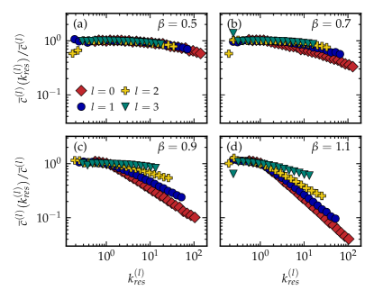
Figure 2: The flow of the rescaled average local clustering coefficient per rescaled degree class under the randomized coarse-graining scheme for different $\beta^{\prime}s$: (a) $\beta=0.5$, (b) $\beta=0.7$, (c) $\beta=0.9$, (d) $\beta=1.1$. Here, $l=0$ represents the original network and we perform three consecutive renormalization steps with $r=2$, leading to the cases $l=1,2$ and $3$. The network parameters used to generate the original networks are $\{N,\gamma,\langle k\rangle\}=\{65536,2.9,6\}$.

We first study self-similarity of the clustering spectrum as clustering is the key property of geometric graphs due to its relation to the triangle inequality. In Fig. 1, it is shown that, for a scale-free synthetic network with $\beta=0.8$, GR reveals self-similar behavior in the renormalization flow. In Fig. 2, we show the results for the randomized coarse-graining scheme. We see that self-similarity is obtained for the smallest $\beta$’s, implying that geometric information is not important here. However, the overlap between the different curves gets progressively worse as $\beta$ increases, reflecting the growing importance of the geometry. The self-similarity is lost at $\beta\approx 0.7$, very close to the theoretical transition point $\beta_{c}^{\prime}=2/\gamma$ between the non- and quasi-geometric regimes [22]. The curves flatten out with $l$, implying that more and more of the clustering in the network is due to high degree nodes. This is to be expected, as the random coarse-graining scheme destroys the coupling of the network to the geometry. This leads to networks that are similar to those generated with the configuration model, where we know that most of the clustering is due to high degree nodes [27].

Figure 3: (a,b) The flow of the connection probability as a function of $\chi=x_{nm}^{\beta}/(\hat{\mu}\kappa_{n}\kappa_{m})^{\max(1,\beta)}$ under the RGN where nodes are combined sequentially (a) or randomly (b) along the circle. The dotted lines give the theoretical curve. (c) The mean difference between the two previous cases for $l=1$ and for three different $\gamma$’s. In all cases the networks were generated with the $\mathbb{S}^{1}$ model with $N=65536$ and $\langle k\rangle=6$.

To quantify further how much poorer the results of the randomized coarse-graining scheme are in comparison to GR, we measured how well the empirical connection probability of the renormalized network fits the theoretical one in the $\mathbb{S}^{1}$-model. After obtaining the hidden coordinates, the parameter $\chi_{ij}=x_{ij}^{\beta}/(\hat{\mu}\kappa_{i}\kappa_{j})^{\max(1,\beta)}$ were determined for each pair of nodes. These values were binned logarithmically, and for each bin the proportion of links versus non-links was calculated to produce the inferred connection probability $p(\chi)$. The results of this analysis are shown in Fig. 3 where we have used networks in the quasi-geometric regime with $\beta=0.8$. Fig. 3a shows the inferred connection probability of the different renormalized layers for the standard GR, where geometric information is used to define the supernodes. In Fig. 3b, we see the same results but for the case where the nodes are chosen at random. Clearly, while GR produces self-similar copies congruent with the $\mathbb{S}^{1}$ connection probability, the random procedure does not. This confirms that in the quasi-geometric regime geometric information is important even though the geometric coupling is weak.

Figure 4: The degree distribution and rescaled average local clustering coefficient as functions of the rescaled degree for (a,b) the genetic multiplex of the yeast S.cerevisiae, (c,d) the Human protein-protein interaction network and (e,f) the interaction network of users on the online Q&A site MathOverflow. For this last network, the $\mathbb{H}^{2}$ representations of the (g) original ($l=0$) and (h) renormalized ($l=3$) networks are shown. The details of these networks are given in the SM [26].

We plot the average difference between the connection probabilities of the two schemes at layer $l=1$ as a function of the inverse temperature $\beta$ in Fig. 3c. To compute this difference, one first samples parameters $\chi_{ij}^{(l=1)}$ logarithmically. For each of these values, one finds the observed connection probability for the two schemes. One then takes the difference between these cases and averages this over the sampled distances. Once again, three different behaviors can be observed. In the geometric regime ($\beta>1$), the difference between the two methods is large. For $\beta$’s in the quasi-geometric regime, the difference decreases, and it goes to zero in the non-geometric regime. The transition point between the non- and quasi-geometric regimes shifts to higher betas when the heterogeneity of the network is increased, in line with the theoretical prediction that this transition occurs at $\beta_{c}^{\prime}=2/\gamma$ [22]. The discrepancy between the curves at $\beta>1$ comes from the fact that not only similarity but also popularity plays a role in the connection probability. As this second type of information is used equivalently in the renormalization procedure regardless of how the angular coordinates are chosen, the difference between these two methods can thus be expected to be smaller when popularity dimensions plays a more important role, which is the case when the degree distribution is more heterogeneous, i.e. when $\gamma$ is smaller.

Now that we have set up the renormalization procedure $\beta<1$ and shown that geometric information is relevant in this regime, we are able to study the self-similarity of real networks that are best described as being weakly geometric [21]. In Fig. 4e-f the degree distribution and clustering spectrum of several of those real networks and their scaled-down replicas are shown. In particular, we study the genetic multiplex of the nematode worm C. Elegans (Fig. 4a,b) [28], the human protein-protein interaction network (Fig. 4c,d) [29] and the interaction network of users on the online Q&A site MathOverflow (Fig. 4e,f) [30]. The embeddings of these networks in the quasi-geometric domain were produce with the tool provided in [21]. Further details about the networks can be found in Supplementary Information III [26].

In all cases, the curves remain invariant under repeated application of GR. Only for large $l$ does the degree distribution tend to a more homogeneous distribution. This is once again a finite size effect. For the MathOverflow network, we show the $\mathbb{H}^{2}$ representation of the original (Fig. 4g) and scaled-down (Fig. 4h) networks. To obtain the scaled-down replica, GR with $r=2$ was performed thrice, such that the replica was $2^{3}=8$ times smaller than the original. We report similar results for a wide range of other networks in the Supplementary Information IV [26].

In summary, we have extended the geometric renormalization scheme to networks in the weakly geometric regime. We have shown that also in this regime, self-similar scaled-down network replicas can be obtained, where self-similarity refers to important network properties such as the degree distribution and the clustering spectrum. In the quasi-geometric domain $0.5\lesssim\beta\leq 1$, one must define supernodes by grouping consecutive nodes along the $\mathbb{S}^{1}$ circle in order to obtain self-similarity in the clustering spectrum and in the connection probability. This underlines the importance of geometric information for understanding the network topology even when the geometric coupling is weak. In constrast, for $\beta\lesssim 0.5$ it does not matter how nodes are grouped. This implies that for networks in this domain, the connectivity is solely determined by the degree-distribution, making them effectively non-geometric. Finally, we reveal the scale-invariance of many real networks identified in Ref. [21] as living in the quasi-geometric domain of the weak coupling regime, which can be effectively renormalized using the extended GR scheme. These results prove once again the importance of the geometric renormalization approach to reveal hidden symmetries in real networks.
This work was supported by grant TED2021-129791B-I00 funded by MCIN/AEI/10.13039/501100011033 and the “European Union NextGenerationEU/PRTR”; grant PID2022-137505NB-C22 funded by MCIN/AEI/10.13039/501100011033; Generalitat de Catalunya grant number 2021SGR00856. M.B. acknowledges the ICREA Academia award, funded by the Generalitat de Catalunya.

References

- Täuber [2012] U. C. Täuber, Renormalization group: Applications in statistical physics, Nuclear Physics B - Proceedings Supplements 228, 7 (2012).
- Kadanoff [1966] L. P. Kadanoff, Scaling laws for ising models near , Physics Physique Fizika 2, 263 (1966).
- Watts and Strogatz [1998] D. J. Watts and S. H. Strogatz, Collective dynamics of ‘small-world’ networks, Nature 393, 440 (1998).
- Song et al. [2005] C. Song, S. Havlin, and H. A. Makse, Self-similarity of complex networks, Nature 433, 392 (2005).
- Villegas et al. [2023] P. Villegas, T. Gili, G. Caldarelli, and A. Gabrielli, Laplacian renormalization group for heterogeneous networks, Nature Physics 19, 445 (2023).
- Boguñá et al. [2021] M. Boguñá, I. Bonamassa, M. D. Domenico, S. Havlin, D. Krioukov, and M. Á. Serrano, Network geometry, Nature Reviews Physics 3, 114 (2021).
- Serrano and Boguñá [2022] M. A. Serrano and M. Boguñá, The Shortest Path to Network Geometry: A Practical Guide to Basic Models and Applications, Elements in Structure and Dynamics of Complex Networks (Cambridge University Press, 2022).
- Serrano et al. [2008] M. Á. Serrano, D. Krioukov, and M. Boguñá, Self-similarity of complex networks and hidden metric spaces, Physical Review Letters 100, 078701 (2008).
- Krioukov et al. [2010] D. Krioukov, F. Papadopoulos, M. Kitsak, A. Vahdat, and M. Boguñá, Hyperbolic geometry of complex networks, Phys. Rev. E 82, 036106 (2010).
- Gugelmann et al. [2012] L. Gugelmann, K. Panagiotou, and U. Peter, Random Hyperbolic Graphs: Degree Sequence and Clustering, in Autom Lang Program (ICALP 2012, Part II), LNCS 7392 (2012).
- Candellero and Fountoulakis [2016] E. Candellero and N. Fountoulakis, Clustering and the Hyperbolic Geometry of Complex Networks, Internet Math. 12, 2 (2016).
- Fountoulakis et al. [2021] N. Fountoulakis, P. van der Hoorn, T. Müller, and M. Schepers, Clustering in a hyperbolic model of complex networks, Electron. J. Probab. 26, 1 (2021).
- Abdullah et al. [2017] M. A. Abdullah, N. Fountoulakis, and M. Bode, Typical distances in a geometric model for complex networks, Internet Math. 1, 10.24166/im.13.2017 (2017).
- Friedrich and Krohmer [2018] T. Friedrich and A. Krohmer, On the Diameter of Hyperbolic Random Graphs, SIAM J. Discrete Math. 32, 1314 (2018).
- Müller and Staps [2019] T. Müller and M. Staps, The diameter of KPKVB random graphs, Adv. Appl. Probab. 51, 358 (2019).
- Serrano et al. [2011] M. Á. Serrano, D. Krioukov, and M. Boguñá, Percolation in Self-Similar Networks, Phys. Rev. Lett. 106, 048701 (2011).
- Fountoulakis and Müller [2018] N. Fountoulakis and T. Müller, Law of large numbers for the largest component in a hyperbolic model of complex networks, Ann. Appl. Probab. 28, 607 (2018).
- Kiwi and Mitsche [2018] M. Kiwi and D. Mitsche, Spectral gap of random hyperbolic graphs and related parameters, Ann. Appl. Probab. 28, 941 (2018).
- García-Pérez et al. [2018] G. García-Pérez, M. Boguñá, and M. Á. Serrano, Multiscale unfolding of real networks by geometric renormalization, Nature Physics 14, 583 (2018).
- Zheng et al. [2021] M. Zheng, G. García-Pérez, M. Boguñá, and M. Á. Serrano, Scaling up real networks by geometric branching growth, Proceedings of the National Academy of Sciences 118, 10.1073/pnas.2018994118 (2021).
- van der Kolk et al. [2023] J. van der Kolk, M. Á. Serrano, and M. Boguñá, Random graphs and real networks with weak geometric coupling (2023), arXiv:2312.07416 [physics.soc-ph] .
- van der Kolk et al. [2022] J. van der Kolk, M. Á. Serrano, and M. Boguñá, An anomalous topological phase transition in spatial random graphs, Communications Physics 5, 245 (2022).
- Boguñá et al. [2020] M. Boguñá, D. Krioukov, P. Almagro, and M. Á. Serrano, Small worlds and clustering in spatial networks, Physical Review Research 2, 023040 (2020).
- van der Hoorn et al. [2018] P. van der Hoorn, G. Lippner, and D. Krioukov, Sparse maximum-entropy random graphs with a given power-law degree distribution, Journal of Statistical Physics 173, 806 (2018).
- Jankowski et al. [2023] R. Jankowski, A. Allard, M. Boguñá, and M. Á. Serrano, The d-mercator method for the multidimensional hyperbolic embedding of real networks, Nature Communications 14, 7585 (2023).
- [26] J. van der Kolk, M. Boguñá, and M. Ángeles Serrano, Supplementary information for renormalization of networks with weak geometric coupling.
- Colomer-de Simon and Boguñá [2012] P. Colomer-de Simon and M. Boguñá, Clustering of random scale-free networks, Phys. Rev. E 86, 026120 (2012).
- Domenico et al. [2015] M. D. Domenico, M. A. Porter, and A. Arenas, Muxviz: a tool for multilayer analysis and visualization of networks, Journal of Complex Networks 3, 159 (2015).
- Hu et al. [2018] Y. Hu, A. Vinayagam, A. Nand, A. Comjean, V. Chung, T. Hao, S. E. Mohr, and N. Perrimon, Molecular interaction search tool (mist): an integrated resource for mining gene and protein interaction data, Nucleic Acids Research 46, D567 (2018).
- Paranjape et al. [2017] A. Paranjape, A. R. Benson, and J. Leskovec, Motifs in temporal networks (ACM, 2017) pp. 601–610.