ERASE: Benchmarking Feature Selection Methods for Deep Recommender Systems

Abstract.

Deep Recommender Systems (DRS) are increasingly dependent on a large number of feature fields for more precise recommendations. Effective feature selection methods are consequently becoming critical for further enhancing the accuracy and optimizing storage efficiencies to align with the deployment demands. This research area, particularly in the context of DRS, is nascent and faces three core challenges. Firstly, variant experimental setups across research papers often yield unfair comparisons, obscuring practical insights. Secondly, the existing literature’s lack of detailed analysis on selection attributes, based on large-scale datasets and a thorough comparison among selection techniques and DRS backbones, restricts the generalizability of findings and impedes deployment on DRS. Lastly, research often focuses on comparing the peak performance achievable by feature selection methods, an approach that is typically computationally infeasible for identifying the optimal hyperparameters and overlooks evaluating the robustness and stability of these methods. To bridge these gaps, this paper presents ERASE, a comprehensive bEnchmaRk for feAture SElection for DRS. ERASE comprises a thorough evaluation of eleven feature selection methods, covering both traditional and deep learning approaches, across four public datasets, private industrial datasets, and a real-world commercial platform, achieving significant enhancement. Our code is available online for ease of reproduction.

1. Introduction

Recommender systems have become indispensable in many sectors ranging from e-commence to content streaming in the realm of information explosion (Rendle et al., 2009; Rendle, 2010). With the application of deep learning techniques, Deep Recommender System (DRS) exhibits amplified prediction ability of user preference, providing personalized experience and dominating the deployment landscape (Cheng et al., 2016; Wang et al., 2017; Guo et al., 2017).

To improve the accuracy of recommendations, DRS is progressively integrating an expanding array of feature fields into their predictive models, which can number in the hundreds or even thousands (Heaton, 2016). The significance of each feature varies, resulting in the accumulation of superfluous or extraneous features. Consequently, feature selection, which concentrates on pinpointing and leveraging the most critical features, is becoming increasingly crucial in modern DRS (Zheng et al., 2023; Chen et al., 2022). One immediate benefit of feature selection is the enhancement of prediction performance, achieved by eliminating non-contributory features that could otherwise adversely affect predictions. From an industrial viewpoint, selecting predictive features is also essential for meeting deployment criteria regarding memory usage since unnecessary storage demands can often be inflated by the presence of redundant features.

Hand-crafted featrue selection usually requires lots of expert knowledge and labor efforts, which is usually infeasible to achieve the optimal results when the candidate set contains thousands of features. Researchers have invised various methods to automatically select predictive features, including statistical methods (Tibshirani, 1996; Liu and Setiono, 1995; Vergara and Estévez, 2014), learning methods (Chen and Guestrin, 2016; Friedman, 2001; Breiman, 2001), and agent-based methods (Liu et al., 2019; Fan et al., 2020; Zhao et al., 2020).

Despite these methods achieving good results in feature selection, they also reveal the following issues that hinder the development of this field. 1) Experimental Differences. Recent years have witnessed a variety of methods designed for DRS (Wang et al., 2022; Lin et al., 2022; Guo et al., 2022; Lee et al., 2023; Lyu et al., 2023; Zhang et al., 2023; Wang et al., 2023). However, these works conduct experiments with varied settings. For example, MultiSFS (Wang et al., 2023) is designed to select features for multi-taske DRS. SHARK (Zhang et al., 2023) suggests the feature selection method F-permutation together with a quantization method. Optfs (Lyu et al., 2023) selects the feature from the value-level while others mainly select from the field-level. These experimental differences usually lead to the unfair or unavailable comparison, making the subsequent researchers stuggling to generate practical insights. 2) Insufficiency. Existing feature selection benchmarks are predominantly tailored for conventional downstream tasks, such as classification (Bolón-Canedo et al., 2014; Bommert et al., 2020). They are primarily built upon synthetic or domain-specific datasets (Bolón-Canedo et al., 2013; Forman, 2003; Darshan and Jaidhar, 2018), which diverges significantly from the complex, large-scale datasets encountered in DRS. This divergence results in a notable deficiency in guiding feature selection specifically for DRS, due to the benchmarks’ disparate scope and focus. DeepLasso (Cherepanova et al., 2023), while being among the benchmarks most closely related to DRS, primarily addresses tabular learning—a context that, despite similarities, does not fully align with the intricacies of recommendation tasks. Furthermore, such benchmarks often limit their exploration to traditional selection methods and rely on datasets of a much smaller scale than those typically associated with DRS, thereby omitting crucial, in-depth analysis from an industrial perspective. Moreover, while related literature surveys (Chen et al., 2022; Zheng et al., 2023) provide comprehensive reviews of the field, they fall short in offering empirical evidence or experimental results that could motivate practical deployments in DRS, lacking the necessary data-driven support to inform and inspire future research directions. 3) Assessment Deficit. A pivotal hyperparameter in the realm of feature selection is the number of features to be selected, denoted as $k$ in this study. Feature selection methods often exhibit variability in performance across different values of $k$, and it is common that the optimal $k$ varies from one method to another (Wang et al., 2022; Lin et al., 2022; Lyu et al., 2023). This variability introduces two significant challenges in evaluating feature selection methods comprehensively. First, the direct comparison of methods at their respective optimal $k$ may not constitute a fair assessment. Such comparisons fail to account for the different memory requirements associated with varying optimal $k$ values for different selection methods. Furthermore, this approach neglects the performance variability under sub-optimal hyperparameter settings, thereby obscuring insights into the methods’ robustness and stability across a range of $k$ values. Second, the exhaustive search for the optimal $k$ across the entire spectrum of possible values is both time-consuming and computationally intensive. This necessitates an evaluation methodology capable of effectively assessing a method’s performance based on partial $k$ values, offering a more efficient means to gauge feature selection effectiveness without finishing complete iterations.

To address these issues, we propose ERASE, a comprehensive bEnchmaRk for feAture Selection for DRS. ERASE initiates a unified and fair experimental framework, minimizing experimental discrepancies across various selection methods. Remarkably, ERASE pioneers as the first feature selection benchmark with a focus on DRS tasks, incorporating both prevalent DRS feature selection techniques and conventional methods. It introduces a novel taxonomy to classify these methods and unearth intrinsic patterns among groups of methods. By evaluating the performance on widely used public datasets and authentic industrial production datasets—through both offline comparison and online testing—ERASE furnishes strong empirical support, facilitating the generation of actionable insights. In its endeavor to provide a comprehensive assessment of feature selection methods, ERASE contrasts the optimal performance of compared selection methods alongside their outcomes under specific deployment prerequisites. Additionally, we introduce a novel metric, AUKC, specifically crafted for assessing the robustness and stability of feature selection methods across a range of feature quantities $k$, thereby addressing the critical lack of such evaluative metrics. We summarize our major contributions as follows:

• We present ERASE, a comprehensive benchmark for DRS feature selection methods, providing the fair comparison for emerging selection techniques with various datasets and DRS backbones. To the best of our knowledge, we are the first to focus on benchmarking feature selection methods for recoomendation tasks.

• We recognize the assessment shortfall linked to the substantial dependency of selection efficacy on the hyperparameter $k$, and in response, we introduce a novel evaluation metric, AUKC. This metric is designed to evaluate the robustness and stability of feature selection methods, bridging the existing gap in assessment.

• We carry out thorough experiments across four widely used public datasets and real-world industrial production datasets, yielding insights from various angles. Notably, our experimental findings have guided optimizations in our online platform, achieving a 20% reduction in latency without compromising effectiveness, validating the practical utility of our benchmark.

2. Becnchmark Design

forked edges, for tree= grow=east, reversed=true, anchor=base west, parent anchor=east, child anchor=west, base=left, font=, rectangle, draw=white, rounded corners, align=left, minimum width=1em, edge+=darkgray, line width=1pt, s sep=5pt, l sep=30pt, inner xsep=3pt, inner ysep=3pt, line width=1pt, ver/.style=rotate=90, child anchor=north, parent anchor=south, anchor=center, , [ERASE,leaf-head [ Datasets
(§2.1), leaf-dataset,text width=5em [ Avazu, modelnode-dataset, text width=8em ] [ Criteo, modelnode-dataset, text width=8em ] [ Movielens-1M, modelnode-dataset, text width=8em ] [ AliCCP, modelnode-dataset, text width=8em ] ] [ Feature
Selection
Methods
(§2.2), leaf-fs,text width=5em [ Shallow
Feature
Selection, leaf-fs, text width=5em [Lasso (Tibshirani, 1996), modelnode-fs, text width=8em] [GBDT (Friedman, 2001), modelnode-fs, text width=8em] [RF (Breiman, 2001), modelnode-fs, text width=8em] [XGBoost (Chen and Guestrin, 2016), modelnode-fs, text width=8em] ] [ Gate-based
Feature
Selection, leaf-fs, text width=5em [AutoField (Wang et al., 2022), modelnode-fs, text width=8em] [AdaFS (Lin et al., 2022), modelnode-fs, text width=8em] [OptFS (Lyu et al., 2023), modelnode-fs, text width=8em] [LPFS (Guo et al., 2022),modelnode-fs, text width=8em] ] [ Sensitivity
-based
Feature
Selection, leaf-fs, text width=5em [Permutation (Fisher et al., 2019), modelnode-fs, text width=8em] [SHARK (Zhang et al., 2023), modelnode-fs, text width=8em] [SFS (Wang et al., 2023), modelnode-fs, text width=8em] ] ] [ Backbone
Models
(§2.3), leaf-bbm,text width=5em [ Wide&Deep (Cheng et al., 2016), modelnode-bbm, text width=8em ] [ DeepFM (Guo et al., 2017),modelnode-bbm, text width=8em] [ DCN (Wang et al., 2017),modelnode-bbm, text width=8em] [ FibiNet (Huang et al., 2019),modelnode-bbm, text width=8em] ] [ Metrics
(§2.4), leaf-metrics,text width=5em [AUC, modelnode-metrics,text width=8em] [Logloss, modelnode-metrics,text width=8em] [AUKC, modelnode-metrics,text width=8em] ] ]

Figure 1. Benchmark Overview.

In this section, we will give an overview of our benchmark. As shown in Figure 1, the benchmark is consisted of four components: dataset, feature selection methods, backbone models, and metrics. Specifically, datasets are crucial experimental foundations for benchmarks. We elaborate on the datasets utilized in Section 2.1. The core introduction to the feature selection methods is presented in Section 2.2. Next, different feature selection methods or the selected features need to apply to specific backbone models, which are discussed in Section 2.3. Finally, in Section 2.4, we provide a detailed description of the evaluation metrics used in this benchmark, including two existing metrics and one newly proposed metric.

2.1. Datasets

To comprehensively evaluate the effectiveness of different feature selection methods, we select four public datasets for our experiments. Avazu and Criteo are selected because they are frequently used dataset for studying feature selection in DRS (Wang et al., 2022; Lin et al., 2022; Lyu et al., 2023). To compare the performance of different methods with a small feature set, we choose the popular Movielens-1M dataset in the recommendation field. Additionally, to compare the performance of different methods in scenarios closer to real-world recommender systems, we supplement with the AliCCP dataset, which possesses user and item features and includes a rich set of 85,316,519 interaction samples. The statistics of datasets and the detailed introduction of datasets are illustrated in Appendix A.

2.2. Feature Selection Methods

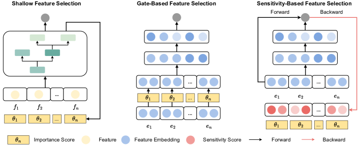
Figure 2. Overview of three categories of feature selection methods in deep recommender systems.

Table 1. Methods Overview. For the type column, ”Shallow” represents shallow feature selection methods, ”Gate” represents gate-based feature selection methods, and ”Sensitivity” represents the sensitivity-based feature selection methods. For the single-stage, two-stage, soft selection, and hard selection columns, ✔ represents applicable, ✘ represents not applicable, and ✔$\star$ represents that this method can be applicable after appropriate modifications.

Methods	Type	Single-stage	Two-stage	Soft Selection	Hard Selection
Lasso	Shallow	✘	✔	✘	✔
GBDT	Shallow	✘	✔	✘	✔
RF	Shallow	✘	✔	✘	✔
XGBoost	Shallow	✘	✔	✘	✔
AutoField	Gate	✘	✔	✘	✔
AdaFS	Gate	✔	✘	✔	✘
OptFS	Gate	✘	✔	✔	✔$\star$
LPFS	Gate	✔	✔$\star$	✔	✔$\star$
Permutation	Sensitivity	✘	✔	✘	✔
SHARK	Sensitivity	✘	✔	✘	✔
SFS	Sensitivity	✘	✔	✘	✔

We list all feature selection methods in this work and their attributes in Table 1. There are three feasible dimensions to classify these methods. 1) Training strategy. Based on the training strategy, the methods can be single-stage or two-stage. Single-stage usually integrates the feature selection module directly into the original model without changing the training logic. In contrast, two-stage methods contain searching and retraining phases. Informative feature fields or feature values are selected in the searching phase, and the backbone model is trained with these selected features in the retraining phase. 2) Selection type. There are two types of selection in feature selection methods: soft selection and hard selection. The soft selection offers a mask to affect inputs. Features multiplied with 0 are considered filtered out. For the hard selection, features are removed directly from the inputs. 3) Selection technique. Depending on the techniques used for selection, as shown in Figure 2, we divide methods contained in our benchmark into three categories: shallow feature selection, gate-based selection, and sensitivity-based selection. Shallow selection methods, including Lasso (Tibshirani, 1996), GBDT (Friedman, 2001), RandomForest (RF) (Breiman, 2001) and XGBoost (Chen and Guestrin, 2016), select features based on the feature importance score derived from the shallow learning methods (e.g., RandomForest). Gate-based methods, including AutoField (Wang et al., 2022), AdaFS (Lin et al., 2022), OptFS (Lyu et al., 2023), and LPFS (Guo et al., 2022), distribute gates to control the usage of features and decide the selection results according to gate outputs. Sensitivity-based methods, including Permutation (Fisher et al., 2019), SHARK (Zhang et al., 2023), and SFS (Wang et al., 2023), compute the feature importance by measuring the sensitivity of gradients to features. Due to the unbalanced distribution of feature selection methods classifying on training strategy and selection type, we elaborate our work based on selection technique classification. The detailed introduction of these methods is in Appendix B.

2.3. Backbone Models

To comprehensively evaluate the effectiveness of feature selection methods, we choose four popular DRS models as backbones: 1) Wide&Deep: A classical model contains shallow and deep networks to capture feature interactions. 2) DeepFM: A model with FM module to automatically learn feature interactions. 3) DCN: A model with cross layers to study feature interactions. 4) FibiNet: A model equipped with SENet and bilinear layer to adaptively learns feature importance and captures high-order feature interactions. The detailed introduction of these models are in Appendix C.

2.4. Metrics

In this paper, we focus on the Click-Through Rate (CTR) prediction task, so we take AUC and Logloss as the two main metrics in our benchmark, the detailed introduction is in Appendix E. Additionally, since there is currently no metric that comprehensively evaluates the performance of feature selection methods across varying numbers of selected features, we propose a new evaluation metric named “AUKC” to address this challenge.

AUKC. Current metrics cannot assess the robustness and stability of a specific feature selection method across different numbers of selections. Therefore, we introduce a new metric Area Under the $K$-performance Curve (AUKC) to fill this gap. AUKC measures the area under the performance curve of feature selection methods with different $K$. Specifically, AUKC is formalized as follows:

(1) $$AUKC=\frac{1}{|K|}\sum_{k=1}^{|K|}(AUC_{k}+AUC_{k-1}-1)$$

where $|K|$ denotes the number of all feature fields, $AUC_{k}$ is the AUC score when selecting $k$ feature fields follow a specific feature selecting method. If there is no input features, the model would make random predictions so that $AUC_{0}=0.5$.

In practice, due to resource contrains, it is generally not feasible to conduct experiments with every possible number of selections. Therefore, we further propose a more general form of AUKC to accommodate this change:

(2) $$AUKC=\frac{1}{|K|}\sum_{n=1}^{|N|}(AUC_{n,l}+AUC_{n,r}-1)\times\Delta l_{n}$$

where $|K|$ denotes the number of all feature fields, $|N|$ is the number of segments across the entire length of the feature fields set. $AUC_{n,l}$ is the AUC corresponding to the number of features selected at the left endpoint of the $n$-th segment, and $AUC_{n,r}$ denotes the AUC with the number of selections at the right endpoint of the $n$th segment. $\Delta l_{n}$ represents the length of the $n$-th segment. The detailed process of the formula derivation is in the Appendix F.

AUKC and AUC share a similar conceptual basis, representing the area under a curve, and both have a value range from 0 to 1. However, unlike AUC, the endpoint of AUKC does not necessarily equal 1, and the values in the middle of the curve can exceed the endpoint value. This occurs because eliminating features with less information can result in a model that performs better than one using all available features. The AUKC metric takes into account the effectiveness of feature selection at different numbers of selected features, $k$, thereby providing a more comprehensive reflection of the efficacy of feature selection methods.

3. Experiments

Table 2. Overall experimental results of feature selection for DeepFM and Wide&Deep backbones.

Backbone model	Methods	Avazu		Criteo		Movielens-1M		AliCCP
		AUC	Logloss	AUC	Logloss	AUC	Logloss	AUC	Logloss
DeepFM	no_selection	0.78576	0.37680	0.80024	0.45321	0.79027	0.54124	0.61813	0.16176
	Lasso	0.78587	0.37654	0.79832	0.45483	0.80683	0.52498	0.61887	0.16174
	GBDT	0.76930	0.38571	0.80011	0.45329	0.78942	0.54234	0.61864	0.16150
	RF	0.78642	0.37630	0.79920	0.45427	0.78920	0.54217	0.61772	0.16172
	XGBoost	0.76953	0.38548	0.80022	0.45333	0.78974	0.54190	0.61822	0.16172
	AutoField	0.78611	0.37641	0.80022	0.45325	0.80722	0.52471	0.61894	0.16174
	AdaFS	0.78278	0.37922	0.79950	0.45405	0.78590	0.54676	0.61726	0.16158
	OptFS	0.78624	0.37627	0.79934	0.45505	0.79027	0.54124	0.61551	0.16195
	LPFS	0.78840	0.37601	0.80080	0.45364	0.78885	0.54276	0.61941	0.17864
	Permutation	0.78624	0.37640	0.80006	0.45349	0.78974	0.54207	0.61844	0.16174
	SHARK	0.78611	0.37643	0.80035	0.45329	0.78888	0.54342	0.61840	0.16174
	SFS	0.78626	0.37631	0.80020	0.45330	0.78982	0.54194	0.61835	0.16168
Wide&Deep	no_selection	0.78574	0.37679	0.79971	0.45346	0.79041	0.54163	0.62137	0.16154
	Lasso	0.78578	0.37665	0.79761	0.45526	0.80750	0.52400	0.62096	0.16159
	GBDT	0.76900	0.38583	0.79979	0.45337	0.78926	0.54252	0.62187	0.16146
	RF	0.78571	0.37664	0.79907	0.45400	0.78992	0.54170	0.62202	0.16132
	XGBoost	0.76886	0.38587	0.80023	0.45320	0.78893	0.54266	0.62174	0.16142
	AutoField	0.78601	0.37653	0.79971	0.45348	0.80736	0.52496	0.62176	0.16134
	AdaFS	0.78607	0.37665	0.79952	0.45394	0.78703	0.54467	0.62106	0.16123
	OptFS	0.78582	0.37654	0.80111	0.45284	0.79041	0.54163	0.62053	0.16144
	LPFS	0.78606	0.37680	0.79953	0.45477	0.79072	0.54136	0.61916	0.17177
	Permutation	0.78607	0.37647	0.79988	0.45342	0.78936	0.54226	0.62156	0.16138
	SHARK	0.78592	0.37655	0.80019	0.45313	0.78980	0.54146	0.62148	0.16154
	SFS	0.78592	0.37646	0.80010	0.45326	0.78993	0.54139	0.62165	0.16122

In this section, the following research questions will be answered:

RQ1: In a fair and unified environment, how do different feature selection methods perform?

RQ2: How do different feature selection methods perform in terms of robustness and stability across various numbers of selections?

RQ3: How is the efficiency of different feature selection methods?

RQ4: Do the performances of feature selection methods align between large-scale industrial datasets and public datasets?

RQ5: Do the performances of various feature selection methods remain consistent online and offline?

Importantly, we also elucidate the congruence among feature rankings derived from various selection methods by visualizing their similarities in Appendix J. This analysis aims to explore both the intra- and inter-group relations among the three categories.

3.1. Experimental Details

We implement the benchmark framework based on Pytorch 1.11. In the training phase, we utilize the Adam optimizer with $\beta_{1}=0.9$, $\beta_{2}=0.999$, and $\epsilon=1\times 10^{-8}$. We set the learning rate as 0.001, the batch size as 4,096, and the embedding size as 8. For the activation function, if the original papers do not emphasize a specific one, we use ReLU as the activation function. We release the repository of our benchmark online. The details of reproduction and hyperparameters for specific backbone models and feature selection methods are illustrated in Appendix D and Appendix G. We conduct each experimental setting three times and record its average metrics to mitigate the impact of experimental fluctuations.

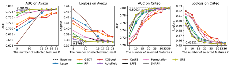
Figure 3. Experimental results of feature selection methods with DeepFM backbone, evaluated by AUC and Logloss.

3.2. Overall Performance (RQ1)

Table 3. Experimental results of AUKC on Avazu and Criteo.

Methods		Lasso	GBDT	RF	XGBoost	AutoField	OptFS	LPFS	Permutation	SHARK	SFS
Avazu	DeepFM	0.43896	0.44430	0.49814	0.43264	0.50526	0.40455	0.49337	0.48526	0.50267	0.50146
	WideDeep	0.43845	0.44392	0.49780	0.43271	0.50537	0.40464	0.49349	0.48521	0.50254	0.50120
	DCN	0.43909	0.44419	0.49920	0.43311	0.50658	0.40534	0.49472	0.48673	0.50363	0.50223
	FibiNet	0.44410	0.44626	0.50475	0.43544	0.50877	0.40974	0.49866	0.49246	0.50918	0.50691
Criteo	DeepFM	0.52193	0.49894	0.52498	0.49388	0.53862	0.50410	0.53634	0.50311	0.53886	0.53998
	WideDeep	0.52142	0.49821	0.52473	0.49338	0.53826	0.50369	0.53598	0.50279	0.53857	0.53972
	DCN	0.52245	0.49898	0.52582	0.49410	0.53926	0.50449	0.53690	0.50374	0.53952	0.54077
	FibiNet	0.52822	0.50459	0.53155	0.50006	0.54528	0.51048	0.54329	0.50964	0.54580	0.54693

Overall experimental results with different backbone models. In this subsection, we compare the performance of feature selection methods with different backbone models. The complete experimental results for all four backbone models are illustrated in Appendix H. For the two-stage approaches (Lasso, GBDT, RF, XGBoost, AutoField, Permutation, SHARK, and SFS), we experiment with different values of selected features during the retraining stage and adopt the best results. In the case of the single-stage approach, if it can also be modified to a two-stage method (OptFS and LPFS), we conduct experiments on both ways and record the optimal results; if it only supports single-stage (i.e., AdaFS), we directly document its results. From Table 2, we can observe the following points:

• In general, gate-based methods show better performance compared to shallow feature selection and sensitivity-based feature selection. The likely reason is that compared to using traditional machine learning methods or solely relying on gradient information, leveraging the powerful expression and learning capabilities of deep neural networks allows for a more thorough exploration of feature importance.

• The effectiveness of feature selection methods remains relatively consistent across different backbone models. This is because the information contained in feature combinations is objective and factual and is not affected by the backbone model.

• The validity of feature selection methods is distinct across different datasets. The shallow feature selection methods perform better in Criteo and Aliccp. The possible reason is the feature value distribution in the other two datasets is very imbalanced, making shallow models prone to overfitting. Gate-based feature selection methods are good at dealing with limited data, while sensitivity-based feature selection methods achieve the best performance among all methods in datasets with rich samples. This finding can be attributed to the fact that in the data-scare scenario, gradients are too sensitive to judge feature importance. However, with sufficient data support, the stability of gradient information will be greatly improved, allowing for more accurate feature importance rankings.

• The two-stage approach yields more stable results compared to the single-stage method across different backbone models. This is because the feature combinations filtered out by the two-stage method can exist independently after the search phase, whereas the single-stage method requires retraining the feature importance scores with each training session.

3.3. Effects on Number of Selection (RQ2)

Overall experimental results with different number of selected features. In this subsection, we conduct experiments on each backbone model and use the different number of selected features $K$. Figure 3 shows the effects of the number of selected features with feature selection methods. The x-axis represents the number of selected features $K$ and the y-axis represents the evaluation metrics AUC or Logloss. We only visualize the results by taking DeepFM as the backbone model here, for we find that the trends for different backbone models remain consistent. The detailed experimental results for the other backbone models are listed in Appendix I. In addition, it is worth noting that to make OptFS applicable in this experiment, we follow the drop rates of feature values in each feature field to assign importance scores to features. From Figure 3, we can find the following information:

• The effectiveness of features selected by different methods varies in ranking when the number of selections changes. Specifically, when the number of features selected is smaller (i.e., 5 or 10), Autofield, SHARK, and SFS perform better. They obtain information through the values or gradients of gate vectors, guiding the sorting of feature importance. They are good at selecting the most informative features from the candidate feature sets. OptFS initially performs not good, as it is inherently a single-stage method. Modifying it to a two-stage method based on different feature value drop rates may not align with the goal of enhancing effectiveness through feature selection. When the number of features approaches the full set of features, the Permutation method performs well. This is because the permutation method calculates feature importance scores based on the loss of effect caused by dropping a feature from the full set. It tends to identify redundant features with less information.

• The XGBoost and GBDT methods show different trends on the Avazu and Criteo datasets. Specifically, they perform poorly on the Avazu dataset but well on the Criteo dataset. This is because the Avazu dataset’s feature values are concentrated in a few feature fields, leading to an imbalance that makes XGBoost and GBDT prone to overfitting, which affects the assessment of feature importance (Strobl et al., 2007).

Experimental results of AUKC. To compare the robustness and stability of feature selection methods across different numbers of selections, we evaluate the selection results with the AUKC metric. Table 3 shows the experimental results of AUKC on Avazu and Criteo. We can draw the following points: 1) Overall, sensitivity-based feature selection methods outperform gate-based feature selection methods, which are superior to shallow feature selection methods. The possible reason is that gradient-based methods calculate feature importance based on partial batches, which helps prevent overfitting. The inferior performance of shallow feature selection methods may be due to the simplicity of the models, which cannot effectively capture the complex relationships between features to determine feature importance. 2) Regarding specific methods, AutoField, SHARK, and SFS exhibit the best performance, demonstrating leading effects across different datasets. It is noteworthy that AutoField significantly surpasses other gate-based feature selection methods. This may be attributed to AutoField being trained in a bi-level optimization manner, which reduces the risk of overfitting, making the selection results more stable and reliable. In conclusion, AutoField, SHARK, and SFS are superior to the other methods on the robustness and stability across different numbers of selections.

Table 4. Experimental results with performance limitations.

FS Methods	Avazu		Criteo
	memory remain	$K$	memory remain	$K$
Lasso	99.99963%	17	68.73103%	25
GBDT	100.00000%	23	23.22062%	30
RF	99.99161%	10	99.56109%	20
XGBoost	100.00000%	23	75.20371%	33
AutoField	99.91556%	10	8.17985%	20
AdaFS	100.00000%	23	100.00000%	39
OptFS	99.73494%	17	79.05157%	25
LPFS	99.96204%	15	0.00100%	15
Permutation	71.56409%	15	48.77971%	25
SHARK	99.98986%	10	7.31463%	15
SFS	99.98345%	10	8.16199%	15

3.4. Efficiency Analysis (RQ3)

In this subsection, we answer the RQ3 from two aspects: experiments with performance limitations and with memory limitations.

3.4.1. Experiments with performance limitations

In real-world scenarios, an important consideration is reducing the memory usage of a model as much as possible while ensuring its effectiveness. To test the memory-saving capabilities of different methods under the constraint of maintaining effectiveness, experiments were conducted on two classic DRS datasets, Avazu and Criteo, using DCN as the backbone model. Firstly, we calculate an acceptable threshold for effectiveness based on the baseline performance of the backbone model (without feature selection, using the full set of features), considering a 1% loss in AUC as acceptable. The threshold is AUC 0.77873 for Avazu and AUC 0.79245 for Criteo. Based on the feature importance ranking list obtained in the search phase by different feature selection methods, we select features from highest to lowest importance until the model’s performance exceeds the threshold. We record the number of features and feature values required to reach this lower threshold of effectiveness for each feature selection method. Since most parameters in DRS models are concentrated in the embedding table, we only considered the memory usage of the embedding table when calculating the memory models required. From Table 4, we can conclude that:

• From the perspective of memory usage, methods like AutoField, LPFS, Permutation, SHARK, and SFS perform better. This indicates that even in DRS scenarios rich in high-dimensional sparse features, these methods do not rely solely on ID-type features (e.g., userid). Instead, they effectively select informative features. It’s noteworthy that AdaFS shows 100% memory usage on both datasets. This is because AdaFS is an instance-level selection method (where gate weights vary with each input sample), and therefore cannot save memory usage.

• In terms of the number of features, RF, AutoField, LPFS, SHARK, and SFS only require half or fewer of the original feature set to achieve 99% of the backbone model’s performance. On the other hand, GBDT and XGBoost need more features. A possible reason for this is that GBDT and XGBoost are prone to overfitting in high-dimensional sparse DRS datasets, which can affect the judgment of feature importance.

• From the perspective of the datasets, the memory-saving effectiveness of various methods is less pronounced on the Avazu dataset compared to the Criteo dataset. This is because most feature values in the Avazu dataset are concentrated in just a few feature fields, whereas in Criteo, the feature values are more evenly distributed. Therefore, when these particular feature fields are indispensable sources of information for CTR prediction, the memory-saving effect becomes less noticeable.

3.4.2. Experiments with memory limitations

Table 5. Experimental results with memory limitations.

FS Methods	25% memory		50% memory		75% memory
	AUC	$K$	AUC	$K$	AUC	$K$
Lasso	0.76513	11	0.76509	12	0.79465	25
GBDT	0.79981	32	0.80003	33	0.80008	34
RF	0.72374	6	0.75961	8	0.76520	10
XGBoost	0.76282	16	0.77942	21	0.78809	30
AutoField	0.79997	30	0.80037	32	0.80037	32
OptFS	0.79162	21	0.79263	22	0.79297	23
LPFS	0.79892	25	0.80015	30	0.80031	32
Permutation	0.79462	24	0.79782	30	0.79782	30
SHARK	0.79748	20	0.79977	25	0.79977	25
SFS	0.79577	18	0.80027	28	0.80027	28

Maximizing effectiveness within limited memory is also an important application scenario for feature selection. To test the capability of different methods in feature selection under memory constraints, experiments were conducted on the Criteo dataset using DCN as the backbone model. The memory limits were categorized into three levels: 25% memory, 50% memory, and 75% memory. Specifically, since the parameters in DRS are mostly concentrated in the embedding table, we used the memory usage of the full feature set’s embedding table as a reference. We set thresholds at 25%, 50%, and 75% of the total memory to record the optimal performance achievable under memory constraints by different feature selection methods. Since AdaFS is incapable of performing a hard selection of partial feature fields, it is not included in this experiment. Based on the results presented in Table 5, we can draw the following conclusion:

• Overall, gate-based feature selection and sensitivity-based feature selection methods perform better. Even when restricted to using only 25% of the available memory, they can achieve results close to those obtained using the full set of features. This is because these methods rely on more powerful deep learning networks that can better model feature importance and are not dependent on high-dimensional sparse ID-type features in DRS.

• Specifically, AutoField achieves the best results because its designed controller effectively learns the importance of each field for the prediction outcome. The DARTS (Differentiable Architecture Search) (Liu et al., 2018) parameter updating manner made the learning of the gate vector more robust and capable of generalization. In contrast, Random Forest (RF) performs the worst. This is because, in the context of high-dimensional sparse DRS, RF tends to assign high weights to ID-type features with numerous feature values. Such feature fields offer more opportunities for splitting, which facilitates the training of RF. However, this approach increases the risk of model overfitting. This tendency of RF to favor features with many splitting points can lead to a bias towards complex, less generalizable models that don’t necessarily capture the most predictive or relevant features for the task at hand.

3.5. Offline Results on Industrial Dataset (RQ4)

To find whether our conslusions for feature selection methods align between large-scale industrial datasets and public datasets, we conduct comparison experiments on large-scale industrial datasets.

3.5.1. Industrial Dataset

The dataset is constructed with CVR records from 2023-11-29 to 2023-11-30 containing approximately seven hundred million samples. Within these samples, The positive sample ratio is 0.196107. The feature used in this offline dataset is aligned with the online service model, which contains 157 features (10 are dense, 36 are sparse, and 111 are multi-hot features). All of these features have been roughly proved useful in offline leave-one-out experiments.

3.5.2. Experiment

Considering the industry dataset is relatively huge, we only select the top 5 elite methods for comparison according to their performance on public datasets, including two gate-based methods (AutoField and LPFS) and three sensitivity-based methods (SHARK, Permutation, and SFS).

The feature preprocessing is slightly different from the public dataset. Specifically, we utilize AutoDis (Guo et al., 2021) technique to directly convert dense features into embeddings with the same size as sparse features. As for multi-hot features, we adopt the reduce-mean operator to aggregate multiple embeddings into one feature embedding. Finally, the preprocessed features are fed into the FibiNet backbone.

After training, we grab each method’s feature importance and perform top-k experiments. The experiment result is demonstrated in Table 6 and Figure 4. From the redundant feature elimination perspective, SHARK, AutoField, and Permutation perform the best. They eliminate about half of the feature sets (80 features) without decreasing model accuracy. However, from the effective feature mining perspective, AutoField performs best for small feature sets, aligning with our observation from the public datasets. We can also find that AutoField achieves the highest AUKC in Table 6, demonstrating its robustness and stability across different numbers of selections. LPFS’s performance is slightly misaligned with the one on the public dataset. We attribute this misalignment to the sensitive learnable polarization module.

3.6. Online Experiments (RQ5)

To validate the effectiveness of our benchmark in online environments, we reconfigure partial benchmarks to adapt to our feature factory, package them into a new toolkit, and conduct online tasks with this toolkit for redundant feature elimination tasks.

Specifically, we create an experiment group that reduces 30% features with our toolkit in a latency-sensitive online recommendation platform. Then, we deploy the experimental group for the A/B test with 5% traffic (approximately 1 million users). After one week’s observation, the inference latency reduces by approximately 20% while the number of video views (vv) and average play duration keeps the same. This experiment proves the effectiveness of our benchmark toolkits in the online environment.

Table 6. Overall experimental results on industrial dataset

Methods	Base	AutoField	LPFS	Permutation	SHARK	SFS
AUC	0.933920	0.933915	0.933858	0.933946	0.933985	0.933894
AUKC	N/A	0.819053	0.817445	0.818387	0.818169	0.817084

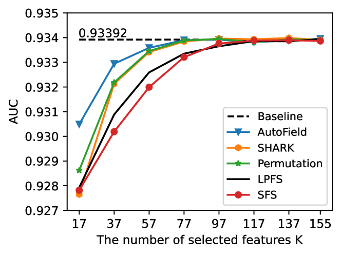
Figure 4. K-performance figure on industrial dataset

4. Related Works

We review the related work from two perspectives, feature selection methods, as well as related benchmarks.

Feature Selection Methods. Traditional feature selection methods fall into three categories: filter, wrapper, and embedded methods (Guyon and Elisseeff, 2003). Filter methods utilize criteria to identify predictive feature fields, exemplified by the Chi2 score (Liu and Setiono, 1995) and mutual information (Vergara and Estévez, 2014). Wrapper methods employ black-box models to select predictive features, assessing the utility of feature subsets through, often, generic algorithms (Granitto et al., 2006; Shah and Kusiak, 2004). Embedded methods, on the other hand, integrate the feature selection process within the prediction model, thereby evaluating the effectiveness of feature subsets in conjunction. Notable embedded methods include LASSO (Tibshirani, 1996) and Gradient Boosting Machine (Friedman, 2001). The advent of deep learning has spurred novel approaches, such as gate-based methods, where learnable gates determine the significance of feature fields (Wang et al., 2022; Lin et al., 2022; Lyu et al., 2023; Lee et al., 2023), and sensitivity-based methods, leveraging gradient techniques to identify critical features by their sensitivity (Zhang et al., 2023; Wang et al., 2023; Fisher et al., 2019). Furthermore, some studies explored reinforcement learning to automate feature selection, using agents to pinpoint predictive features (Liu et al., 2019; Fan et al., 2020; Zhao et al., 2020).

Considering their appliability to DRS, our benchmark focus on traditional embedded methods (termed “shallow methods”), alongside gate-based and sensitivity-based methods. Other techniques often fall short in terms of effectiveness or efficiency within the DRS context. Specifically, filter methods might overlook the DRS model’s nuances by relying solely on data-intrinsic relationships, leading to suboptimal outcomes. Besides, wrapper and reinforcement learning methods, typically designed for smaller datasets, become impractically time-consuming for the expansive datasets characteristic of DRS, which can encompass millions of samples.

Benchmarks for Feature Selection. Most existing benchmarks are tailored for classical downstream models (Bolón-Canedo et al., 2014; Bommert et al., 2020) and rely on synthetic or domain-specific datasets (Bolón-Canedo et al., 2013; Forman, 2003; Darshan and Jaidhar, 2018). Due to their constrained relevance, these benchmarks frequently fall short in providing the necessary guidance to propel research forward in the domain of DRS feature selection. The most related work, DeepLasso (Cherepanova et al., 2023), confines its evaluation to shallow methods and a narrow set of backbone models, primarily targeting tabular learning tasks. Despite utilizing real-world datasets, the scale of these datasets pales in comparison to those encountered in DRS scenarios, thus limiting the provision of actionable insights for DRS feature selection strategies.

ERASE undertakes a thorough evaluation of shallow, gate-based, and sensitivity-based methods across an array of representative DRS backbones, leveraging both large-scale public datasets and private industrial datasets. Furthermore, ERASE proposes a novel metric designed to assess feature selection efficacy comprehensively. Standing as the inaugural comprehensive benchmark for DRS feature selection methodologies, ERASE aims to illuminate effective application strategies for these methods and to chart potential avenues for future research in this domain.

5. Conclusion

In this study, we introduce ERASE, a comprehensive bEnchmaRk for feAture SElection for deep recommender systems (DRS). ERASE integrates a broad spectrum of feature selection methods pertinent to DRS and ensures fair and comprehensive experimentation across four public datasets as well as real-world industrial datasets. Furthermore, ERASE pioneers the adoption of the AUKC metric, devised to address the shortcomings of existing metrics by offering a thorough evaluation of the robustness and stability of feature selection methods over various numbers of selected features. The empirical validation provided by both offline and online analyses on industrial datasets underscores the applicability of our findings in practical settings, offering valuable perspectives on the deployment of feature selection methods within DRS environments.

Appendix A Datasets

Table 7. Dataset statistics

Dataset	Avazu	Criteo	Movielens-1M	AliCCP
Interactions	40,428,967	45,850,617	1,000,209	85,316,519
Users	N/A	N/A	6,040	238,635
Items	N/A	N/A	3,706	467,298
Interaction Type	Click	Click	Rating (1-5)	Click
Feature Num	23	39	9	23

In this subsection, we introduce the datasets utilized in our benchmark. The statistics of these datasets are listed in Table 7. We select the following four datasets for use:

• Avazu. Avazu is a commonly used dataset in the field of feature selection for deep recommendation systems. It consists of 23 features and 40,428,967 interaction records. We divide the dataset into training, validation, and test sets in a 7:2:1 ratio.

• Criteo. Criteo is another frequently used dataset for studying feature selection in Deep Recommendation Systems. The Criteo dataset contains 45,850,617 samples and 39 features, offering a larger number of features. We also adopt a 7:2:1 ratio for dividing the data into training, validation, and test sets to train the model.

• Movielens-1m. The Movielens dataset is a well-known public movie dataset in the field of recommendation systems, featuring multiple variants with different data volumes to meet diverse research needs. We choose the Movielens-1M dataset, which comprises 9 features. The limited number of features presents a greater challenge for feature selection methods. In our experiments with Movielens, we also divide the dataset into training, validation, and test sets according to a 7:2:1 ratio. The interactions with a rating bigger than 3 are considered as positive samples.

• AliCCP. Alibaba Click and Conversion Prediction (AliCCP) dataset is extracted from the real-world e-commerce platform Taobao. It is a popular dataset used for Click-Through Rate (CTR) estimation. It consists of 23 features and 85,316,519 samples, making it an effective tool for evaluating feature selection methods in scenarios closely resembling real advertising contexts. We follow the original AliCCP splitting approach (Ma et al., 2018), allocating 50% of the data for training, with the remaining data split equally into validation and test sets in a 1:1 ratio.

Appendix B Introduction of Feature Selection Methods

Specifically, our benchmark contains the following methods:

B.0.1. Shallow Feature Selection

• Lasso (Tibshirani, 1996). The least absolute shrinkage and selection operator (Lasso) algorithm is a traditional and useful method in machine learning. It performs both variable selection and regularization to improve the model performance.

• GBDT (Friedman, 2001). Gradient-boosted decision tree (GBDT) is a popular algorithm in regression and classification tasks. GBDT achieves superior performance by continually adding trees to fit residuals. By aggregating the feature importance scores from each tree, it also serves as an effective method for feature selection.

• RandomForest (Breiman, 2001) (RF). RandomForest is an efficient method for feature selection. It derives the feature importance by measuring how much each feature decreases the impurity in a tree, commonly using Gini impurity or entropy.

• XGBoost (Chen and Guestrin, 2016). Extreme Gradient Boosting (XGBoost) is an efficient and scalable implementation of the gradient boosting algorithm. It ranks the importance of features by calculating the improvement of every feature on the final performance.

B.0.2. Gate-based Feature Selection

:

• AutoField (Wang et al., 2022). AutoField is the first gate-based feature selection method in the deep recommender system. It designs a novel controller network to generate a 2-dimensional vector determining whether to choose this feature field or not. It is a two-stage method and selects features on the field level.

• AdaFS (Lin et al., 2022). AdaFS is an algorithm that can generate a gate for each feature field adaptively. It is a single-stage method and selects features on the field level.

• OptFS (Lyu et al., 2023). OptFS focuses on the feature value level selection. It trains a scalar for each feature value and continuously strengthens the constraints on sparsity as training progresses.

• LPFS (Guo et al., 2022). LPFS argues that the conclusion that features with smaller weights are less important than those with larger weights may not necessarily be correct. It proposes a kind of smoothed-$l^{0}$ function that can effectively select informative features. It is a single-stage method and focuses on the field level.

B.0.3. Sensitivity-based Feature Selection

:

• Permutation (Fisher et al., 2019). Permutation works by randomly permuting the feature values at a time and measuring how much this permutation affects the performance of the model.

• SHARK (Zhang et al., 2023). Shark takes the novel first-order component of Taylor expansion as the feature importance score for model prediction. It then prunes those features with lower scores from the embedding table to improve model performance and efficiency.

• SFS (Wang et al., 2023). SFS takes the gradients of the gate for each feature field as the feature importance score. It is a two-stage method and selects on the feature field level.

Appendix C Backbone Models

we apply a variety of feature selection methods to the following four popular deep recommendation models in this work.

• Wide&Deep (Cheng et al., 2016). Wide and Deep (Wide&Deep) model is developed by Google to improve the recommender systems. It combines wide and deep models to fit specific feature combinations in large-scale datasets and previously unseen feature combinations through low-dimensional dense embeddings.

• DeepFM (Guo et al., 2017). DeepFM is an effective model in recommender systems. It combines the strengths of FM models and deep neural networks to extract both low-order feature interactions and high-order feature interactions.

• DCN (Wang et al., 2017). The Deep & Cross Network (DCN) model is proposed by Google to capture both explicit and implicit feature interactions for prediction tasks. The cross layers have cross operations that learn complex feature interactions to improve the prediction performance.

• FibiNet (Huang et al., 2019). The Feature Importance and Bilinear feature Interaction NETwork (FibiNet) is an innovative model in CTR prediction. It introduces the SENET and bilinear layer. SENET learns feature importance adaptively and the bilinear layer captures high-order feature interactions.

Appendix D Usage Example

To enhance the credibility and reproducibility of our benchmark, we release a public repository for the convenience of research in related fields. Categorized by usage, current feature selection methods can be divided into two types: single-stage methods and two-stage methods. Detailed usage examples will be provided for these two types subsequently. In addition, in some feature selection methods, there are a few hyperparameters. To facilitate the selection of hyperparameters for optimal results, our repository integrates the automatic tuning framework NNI. With only minimal changes to the NNI configuration file, the best hyperparameter combinations can be conveniently selected.

D.1. Single-stage Methods Usage Example

For single-stage methods (e.g., AdaFS, LPFS), they don’t need the retraining procedure. In our framework, these methods can be easily implemented by the command python fs_run.py –dataset={ } –model={ } –fs={ } –train_or_search=True –retrain=False

D.2. Two-stage Methods Usage Example

For two-stage methods (e.g., Lasso, AutoField, and Permutation), if users are very familiar with the algorithm and dataset they are using and know how many features selected are best for the performance, they can simply complete the searching and retraining with a single command. python fs_run.py –dataset={ } –model={ } –fs={ } –train_or_search=True –retrain=True –k={SelectNum}

In addition, if it is very difficult to directly determine the number of feature selections $k$, then they can run the framework in the normal two-stage manner. First, run different feature selection algorithms to calculate the importance scores of different features. python fs_run.py –dataset={ } –model={ } –fs={ } –train_or_search=True –retrain=False. Then specify different $k$ values to see the impact of the number of features selected on the final result, and take the corresponding result of the optimal k as the final result. python fs_run.py –dataset={ } –model={ } –fs={ } –train_or_search=False –retrain=True –k={SelectNum} –rank_path={ } –read_feature_rank=True

D.3. Parameter Tuning Usage Example

Some feature selection algorithms require hyperparameter tuning, and manually tuning parameters is an extremely time-consuming and laborious process. Therefore, we integrate the AutoML tool NNI in the framework to help select hyperparameters. Users just need to set the parameter names and search range that need to be tuned in the configuration file of the corresponding feature selection method, and then run the NNI service with the following command. python nni_tune.py –dataset={ } –model={ } –fs={ } –train_or_search={ } –retrain={ } –k={SelectNum} –port={ServerPort}

Appendix E Metrics

In this section, we detail the two frequently used metrics in recommender systems: AUC and Logloss.

1) AUC. Area Under the ROC Curve (AUC) measures the area under the ROC curve. The ROC curve is one graph shows that the classification performance of the model under different thresholds. In addition, in random positive-negative pairs, AUC also represents the probability that the model ranks the positive sample with a higher score than the negative one. It can be formalized as follows:

(3) $$AUC=\frac{\sum_{i}^{M}rank_{i}-M(1+M)/2}{M\times N},\ i\in positiveClass$$

where $M$ denotes the number of positive samples and $N$ is the number of negative samples.

2) Logloss. Logloss is also named Binary Cross-Entropy Loss, it is always used in binary classification tasks. The formula for Logloss is described as follows:

(4) $$Logloss=-\frac{1}{N}\sum_{i=1}^{N}[y_{i}log(\hat{y}_{i})+(1-y_{i})log(1-\hat{y_{i}})]$$

where $N$ is the number of samples, $y_{i}$ denotes the predicted label for $i$th sample, and $\hat{y}_{i}$ denotes the ground truth for $i$th sample.

Appendix F Formula Derivation of AUKC

In this section, we detail the formula derivation process of AUKC. AUKC is a comprehensive metric for assessing the AUC performance of a given feature selection method across different numbers of feature selections. Under ideal circumstances, experiments can be conducted for each number of selections to obtain the corresponding AUC metrics, and then derive AUKC:

(5) $$AUKC =\frac{\sum_{k=1}^{|K|}((AUC_{k}-0.5)+(AUC_{k+1}-0.5))/2}{|K|/2}$$

(6) $$=\frac{1}{|K|}\sum_{k=1}^{|K|}(AUC_{k}+AUC_{k+1}-1)$$

where $|K|$ denotes the number of all features, $AUC_{k}$ is the AUC metric with $k$ features selected. When there is no feature selected, the model will predict labels randomly (i.e., $AUC=0.5$). Therefore, we subtract 0.5 from $AUC_{k}$ to obtain the improvement.

When the number of selected features is unevenly distributed across the length of the set of features (e.g., in practice, the granularity of the feature selection number often becomes finer as it approaches the total number of features, and coarser when there are fewer features), AUKC has a more general format:

(7) $$AUKC =\frac{\sum_{n=1}^{|N|}((AUC_{nl}-0.5)+(AUC_{nr}-0.5))\times\Delta l_{n}/2}{|K|/2}$$

(8) $$=\frac{1}{|K|}\sum_{n=1}^{|N|}(AUC_{n,l}+AUC_{n,r}-1)\times\Delta l_{n}$$

where $|N|$ represents the number of segments for the number of features selected across the entire length of the feature set. For example, with 6 features, if experiments are conducted at feature counts of 2,4,5, and 6, then $|N|=4$. $AUC_{n,l}$ is the AUC corresponding to the number of features selected at the left endpoint of the $n$th segment, and $AUC_{n,r}$ denotes the AUC with the number of selections at the right endpoint of the $n$th segment. $\Delta l_{n}$ represents the length of the $n$th segment.

Appendix G Hyperparameters

Table 8. Hyperparameters for Feature Selection Methods

Method	Hyperparameters
Lasso	default parameters in scikit-learn
GBDT	default parameters in scikit-learn
RF	default parameters in scikit-learn
XGBoost	default parameters in scikit-learn
AutoField	update_frequency: 10
AdaFS	pretrain_epoch: 0 update_frequency: 4
OptFS	gamma: 5000
LPFS	epsilon = 0.1 epsilon_update_frequency = 100 epsilon_decay = 0.9978
Permutation	default parameters in scikit-learn
SHARK	None
SFS	num_batch_sampling = 100

As shown in Table 8, in this section, we detail the hyperparameters we utilized in this paper.

Appendix H Complete Overall Performance

Due to page limitations, we can not include the complete overall experimental results in the main content. We list the complete results in Table 9 for reference.

Table 9. Overall experimental results of feature selection for deep recommender systems.

Backbone model	Methods	Avazu		Criteo		Movielens-1M		AliCCP
		AUC	Logloss	AUC	Logloss	AUC	Logloss	AUC	Logloss
DeepFM	no_selection	0.78576	0.37680	0.80024	0.45321	0.79027	0.54124	0.61813	0.16176
	Lasso	0.78587	0.37654	0.79832	0.45483	0.80683	0.52498	0.61887	0.16174
	GBDT	0.76930	0.38571	0.80011	0.45329	0.78942	0.54234	0.61864	0.16150
	RF	0.78642	0.37630	0.79920	0.45427	0.78920	0.54217	0.61772	0.16172
	XGBoost	0.76953	0.38548	0.80022	0.45333	0.78974	0.54190	0.61822	0.16172
	AutoField	0.78611	0.37641	0.80022	0.45325	0.80722	0.52471	0.61894	0.16174
	AdaFS	0.78278	0.37922	0.79950	0.45405	0.78590	0.54676	0.61726	0.16158
	OptFS	0.78624	0.37627	0.79934	0.45505	0.79027	0.54124	0.61551	0.16195
	LPFS	0.78840	0.37601	0.80080	0.45364	0.78885	0.54276	0.61941	0.17864
	Permutation	0.78624	0.37640	0.80006	0.45349	0.78974	0.54207	0.61844	0.16174
	SHARK	0.78611	0.37643	0.80035	0.45329	0.78888	0.54342	0.61840	0.16174
	SFS	0.78626	0.37631	0.80020	0.45330	0.78982	0.54194	0.61835	0.16168
Wide&Deep	no_selection	0.78574	0.37679	0.79971	0.45346	0.79041	0.54163	0.62137	0.16154
	Lasso	0.78578	0.37665	0.79761	0.45526	0.80750	0.52400	0.62096	0.16159
	GBDT	0.76900	0.38583	0.79979	0.45337	0.78926	0.54252	0.62187	0.16146
	RF	0.78571	0.37664	0.79907	0.45400	0.78992	0.54170	0.62202	0.16132
	XGBoost	0.76886	0.38587	0.80023	0.45320	0.78893	0.54266	0.62174	0.16142
	AutoField	0.78601	0.37653	0.79971	0.45348	0.80736	0.52496	0.62176	0.16134
	AdaFS	0.78607	0.37665	0.79952	0.45394	0.78703	0.54467	0.62106	0.16123
	OptFS	0.78582	0.37654	0.80111	0.45284	0.79041	0.54163	0.62053	0.16144
	LPFS	0.78606	0.37680	0.79953	0.45477	0.79072	0.54136	0.61916	0.17177
	Permutation	0.78607	0.37647	0.79988	0.45342	0.78936	0.54226	0.62156	0.16138
	SHARK	0.78592	0.37655	0.80019	0.45313	0.78980	0.54146	0.62148	0.16154
	SFS	0.78592	0.37646	0.80010	0.45326	0.78993	0.54139	0.62165	0.16122
DCN	no_selection	0.78660	0.37615	0.80045	0.45297	0.78966	0.54228	0.62315	0.16134
	Lasso	0.78628	0.37638	0.79860	0.45456	0.80830	0.52367	0.62289	0.16124
	GBDT	0.76926	0.38578	0.80049	0.45299	0.79106	0.54048	0.62318	0.16131
	RF	0.78644	0.37614	0.79978	0.45342	0.79058	0.54058	0.62310	0.16156
	XGBoost	0.76934	0.38565	0.80067	0.45264	0.79102	0.54050	0.62321	0.16131
	AutoField	0.78663	0.37620	0.80051	0.45286	0.80932	0.52226	0.62350	0.16103
	AdaFS	0.78706	0.37597	0.80018	0.45336	0.78792	0.54366	0.62264	0.16122
	OptFS	0.78663	0.37618	0.80164	0.45222	0.78966	0.54228	0.62083	0.16183
	LPFS	0.78686	0.37631	0.80048	0.45349	0.79006	0.54123	0.62202	0.16536
	Permutation	0.78651	0.37616	0.80052	0.45336	0.79047	0.54086	0.62311	0.16116
	SHARK	0.78656	0.37614	0.80063	0.45300	0.79116	0.54019	0.62302	0.16127
	SFS	0.78649	0.37620	0.80066	0.45273	0.79066	0.54067	0.62299	0.16118
FibiNet	no_selection	0.79039	0.37401	0.80528	0.44854	0.78490	1.44348	0.62138	0.16138
	Lasso	0.79057	0.37399	0.80345	0.45012	0.80350	0.56017	0.62147	0.16162
	GBDT	0.77222	0.38403	0.80537	0.44846	0.78213	1.44155	0.62257	0.16145
	RF	0.79053	0.37377	0.80451	0.44917	0.78421	0.61107	0.62166	0.16133
	XGBoost	0.77202	0.38436	0.80554	0.44828	0.78356	1.25796	0.62132	0.16147
	AutoField	0.79068	0.37371	0.80523	0.44864	0.80091	0.54683	0.62272	0.16137
	AdaFS	0.78959	0.37441	0.80439	0.44953	0.78478	0.54911	0.61938	0.16158
	OptFS	0.79059	0.37383	0.80246	0.45159	0.78490	1.44348	0.61958	0.16154
	LPFS	0.79093	0.37385	0.80559	0.44898	0.78790	0.54625	0.61750	0.16797
	Permutation	0.79071	0.37405	0.80515	0.44861	0.78457	0.67354	0.62136	0.16161
	SHARK	0.79078	0.37364	0.80550	0.44833	0.78574	1.33867	0.62198	0.16123
	SFS	0.79068	0.37369	0.80557	0.44826	0.78507	1.20824	0.62219	0.16140

Appendix I Overall Experimental Results

In this section, we supplement the experimental results for the other backbone models with different number of selected features. The results for Avazu dataset are listed in Table 10 and the results for Criteo dataset are listed in Table 11.

Table 10. Experimental results on more backbone models with different number of selected features on Avazu.

Backbone model	Methods	k=5		k=10		k=15		k=17		k=19		k=21		ALL
		AUC	Logloss	AUC	Logloss	AUC	Logloss	AUC	Logloss	AUC	Logloss	AUC	Logloss	AUC	Logloss
DeepFM	Lasso	0.69426	0.41802	0.72784	0.40604	0.76828	0.38646	0.78525	0.37733	0.78529	0.37717	0.78587	0.37654	0.78576	0.37680
	GBDT	0.71987	0.40871	0.74944	0.39549	0.75142	0.39446	0.76058	0.39009	0.76869	0.38616	0.76930	0.38571	0.78576	0.37680
	RF	0.76056	0.39137	0.78529	0.37706	0.78529	0.37698	0.78562	0.37672	0.78551	0.37679	0.78642	0.37630	0.78576	0.37680
	XGBoost	0.70786	0.41366	0.74351	0.39832	0.74825	0.39612	0.74906	0.39569	0.76334	0.38876	0.76953	0.38548	0.78576	0.37680
	AutoField	0.77724	0.38144	0.78479	0.37746	0.78571	0.37683	0.78562	0.37687	0.78556	0.37731	0.78611	0.37641	0.78576	0.37680
	OptFS	0.63468	0.43421	0.70620	0.41452	0.77639	0.38250	0.77996	0.38016	0.78122	0.37936	0.78624	0.37627	0.78576	0.37680
	LPFS	0.76862	0.38592	0.77012	0.38492	0.78244	0.37849	0.78246	0.37889	0.78428	0.37742	0.78612	0.37638	0.78576	0.37680
	Permutation	0.75022	0.39642	0.77228	0.38493	0.77968	0.38030	0.77972	0.38021	0.78570	0.37686	0.78624	0.37640	0.78576	0.37680
	SHARK	0.77015	0.38557	0.78547	0.37692	0.78586	0.37651	0.78596	0.37645	0.78611	0.37643	0.78612	0.37638	0.78576	0.37680
	SFS	0.76930	0.38562	0.78362	0.37789	0.78571	0.37669	0.78588	0.37658	0.78608	0.37643	0.78626	0.37631	0.78576	0.37680
WideDeep	Lasso	0.69380	0.41833	0.72721	0.40626	0.76808	0.38641	0.78547	0.37682	0.78533	0.37700	0.78578	0.37665	0.78574	0.37679
	GBDT	0.71954	0.40883	0.74924	0.39559	0.75118	0.39457	0.76040	0.39017	0.76876	0.38606	0.76900	0.38583	0.78574	0.37679
	RF	0.76042	0.39114	0.78516	0.37706	0.78530	0.37690	0.78531	0.37693	0.78526	0.37691	0.78571	0.37664	0.78574	0.37679
	XGBoost	0.70841	0.41312	0.74354	0.39822	0.74834	0.39610	0.74894	0.39572	0.76293	0.38889	0.76886	0.38587	0.78574	0.37679
	AutoField	0.77704	0.38135	0.78501	0.37713	0.78577	0.37669	0.78601	0.37653	0.78584	0.37658	0.78591	0.37650	0.78574	0.37679
	OptFS	0.63450	0.43426	0.70591	0.41477	0.77696	0.38188	0.78066	0.37952	0.78160	0.37890	0.78582	0.37654	0.78574	0.37679
	LPFS	0.76841	0.38570	0.77049	0.38461	0.78264	0.37819	0.78289	0.37808	0.78407	0.37747	0.78586	0.37655	0.78574	0.37679
	Permutation	0.74999	0.39631	0.77227	0.38468	0.77968	0.38016	0.78003	0.37994	0.78607	0.37647	0.78592	0.37658	0.78574	0.37679
	SHARK	0.77052	0.38504	0.78531	0.37689	0.78570	0.37672	0.78562	0.37667	0.78592	0.37655	0.78564	0.37671	0.78574	0.37679
	SFS	0.76921	0.38536	0.78354	0.37780	0.78551	0.37673	0.78578	0.37659	0.78581	0.37660	0.78592	0.37646	0.78574	0.37679
DCN	Lasso	0.69380	0.41825	0.72742	0.40627	0.76869	0.38608	0.78582	0.37659	0.78609	0.37648	0.78628	0.37638	0.78660	0.37615
	GBDT	0.71976	0.40878	0.74918	0.39570	0.75123	0.39462	0.76052	0.39017	0.76902	0.38593	0.76926	0.38578	0.78660	0.37615
	RF	0.76201	0.39031	0.78574	0.37661	0.78555	0.37680	0.78577	0.37657	0.78580	0.37665	0.78644	0.37614	0.78660	0.37615
	XGBoost	0.70827	0.41321	0.74392	0.39807	0.74849	0.39593	0.74916	0.39566	0.76323	0.38873	0.76934	0.38565	0.78660	0.37615
	AutoField	0.77749	0.38115	0.78601	0.37653	0.78645	0.37645	0.78645	0.37639	0.78663	0.37620	0.78639	0.37637	0.78660	0.37615
	OptFS	0.63468	0.43415	0.70611	0.41474	0.77745	0.38156	0.78129	0.37917	0.78200	0.37866	0.78663	0.37618	0.78660	0.37615
	LPFS	0.76946	0.38531	0.77101	0.38451	0.78330	0.37780	0.78313	0.37786	0.78476	0.37698	0.78648	0.37611	0.78660	0.37615
	Permutation	0.75168	0.39537	0.77302	0.38419	0.78024	0.37997	0.78037	0.37970	0.78635	0.37635	0.78651	0.37616	0.78660	0.37615
	SHARK	0.77067	0.38495	0.78592	0.37654	0.78658	0.37618	0.78654	0.37611	0.78656	0.37614	0.78648	0.37616	0.78660	0.37615
	SFS	0.76979	0.38512	0.78382	0.37768	0.78638	0.37634	0.78641	0.37627	0.78645	0.37627	0.78649	0.37620	0.78660	0.37615
FibiNet	Lasso	0.69545	0.41807	0.73033	0.40494	0.77087	0.38510	0.78980	0.37449	0.78956	0.37493	0.79057	0.37399	0.79039	0.37401
	GBDT	0.71993	0.40884	0.74957	0.39554	0.75198	0.39448	0.76194	0.38961	0.77192	0.38439	0.77222	0.38403	0.79039	0.37401
	RF	0.76362	0.39021	0.78848	0.37523	0.78955	0.37448	0.78978	0.37426	0.78986	0.37439	0.79053	0.37377	0.79039	0.37401
	XGBoost	0.70802	0.41381	0.74488	0.39857	0.75023	0.39505	0.75097	0.39468	0.76543	0.38756	0.77202	0.38436	0.79039	0.37401
	AutoField	0.77213	0.40204	0.78865	0.37536	0.78984	0.37478	0.78990	0.37482	0.79047	0.37397	0.79068	0.37371	0.79039	0.37401
	OptFS	0.63446	0.43427	0.71170	0.41240	0.77762	0.38818	0.78371	0.37904	0.78525	0.37716	0.79059	0.37383	0.79039	0.37401
	LPFS	0.76961	0.38704	0.77204	0.38648	0.78654	0.37600	0.78726	0.37559	0.78843	0.37504	0.79085	0.37356	0.79039	0.37401
	Permutation	0.75263	0.40864	0.77598	0.38366	0.78495	0.37752	0.78516	0.37707	0.79040	0.37410	0.79071	0.37405	0.79039	0.37401
	SHARK	0.77172	0.38873	0.78939	0.37457	0.79017	0.37411	0.79062	0.37382	0.79060	0.37368	0.79078	0.37364	0.79039	0.37401
	SFS	0.76797	0.39383	0.78777	0.37554	0.79044	0.37399	0.79070	0.37378	0.79051	0.37375	0.79068	0.37369	0.79039	0.37401

Table 11. Experimental results on more backbone models with different number of selected features on Criteo.

Backbone model	Methods	k=5		k=10		k=15		k=20		k=25		k=30		k=33		k=36		ALL
		AUC	Logloss	AUC	Logloss	AUC	Logloss	AUC	Logloss	AUC	Logloss	AUC	Logloss	AUC	Logloss	AUC	Logloss	AUC	Logloss
DeepFM	Lasso	0.72479	0.50722	0.75888	0.48580	0.78383	0.46645	0.79016	0.46150	0.79410	0.45813	0.79599	0.45668	0.79649	0.45632	0.79832	0.45483	0.80024	0.45321
	GBDT	0.71672	0.51344	0.72907	0.50557	0.75672	0.48684	0.76984	0.47763	0.78594	0.46518	0.79707	0.45592	0.79961	0.45357	0.80011	0.45329	0.80024	0.45321
	RF	0.72349	0.50737	0.76500	0.48041	0.78634	0.46455	0.79261	0.45962	0.79436	0.45822	0.79628	0.45658	0.79837	0.45492	0.79920	0.45427	0.80024	0.45321
	XGBoost	0.70563	0.51934	0.71730	0.51254	0.76152	0.48315	0.77716	0.47182	0.78417	0.46656	0.78798	0.46362	0.79958	0.45385	0.80022	0.45333	0.80024	0.45321
	AutoField	0.75196	0.49021	0.77773	0.47153	0.78930	0.46226	0.79458	0.45796	0.79726	0.45564	0.79939	0.45391	0.80013	0.45328	0.80022	0.45325	0.80024	0.45321
	OptFS	0.70339	0.52052	0.72922	0.50514	0.76564	0.48014	0.78946	0.46210	0.79395	0.45832	0.79597	0.45676	0.79761	0.45533	0.79821	0.45492	0.80024	0.45321
	LPFS	0.73206	0.50422	0.77973	0.46986	0.79315	0.45939	0.79767	0.45537	0.79859	0.45458	0.80020	0.45313	0.80033	0.45314	0.80017	0.45337	0.80024	0.45321
	Permutation	0.71647	0.51360	0.73042	0.50461	0.75264	0.48947	0.78133	0.46883	0.79410	0.45833	0.79695	0.45594	0.79915	0.45410	0.80006	0.45349	0.80024	0.45321
	SHARK	0.74438	0.49498	0.77622	0.47247	0.79403	0.45841	0.79694	0.45593	0.79953	0.45391	0.79999	0.45348	0.80028	0.45318	0.80035	0.45329	0.80024	0.45321
	SFS	0.74597	0.49403	0.78149	0.46828	0.79177	0.46015	0.79714	0.45586	0.79929	0.45407	0.80003	0.45351	0.80020	0.45330	0.80009	0.45347	0.80024	0.45321
WideDeep	Lasso	0.72431	0.50758	0.75850	0.48617	0.78382	0.46629	0.79037	0.46122	0.79383	0.45834	0.79574	0.45675	0.79607	0.45653	0.79761	0.45526	0.79971	0.45346
	GBDT	0.71670	0.51347	0.72905	0.50566	0.75620	0.48731	0.76897	0.47817	0.78539	0.46553	0.79690	0.45592	0.79900	0.45411	0.79979	0.45337	0.79971	0.45346
	RF	0.72345	0.50725	0.76461	0.48056	0.78596	0.46461	0.79271	0.45922	0.79423	0.45792	0.79632	0.45634	0.79843	0.45448	0.79907	0.45400	0.79971	0.45346
	XGBoost	0.70554	0.51937	0.71739	0.51243	0.76142	0.48327	0.77640	0.47234	0.78369	0.46677	0.78758	0.46371	0.79938	0.45376	0.80023	0.45320	0.79971	0.45346
	AutoField	0.75180	0.49027	0.77770	0.47143	0.78898	0.46241	0.79470	0.45780	0.79722	0.45565	0.79916	0.45399	0.79955	0.45373	0.79971	0.45348	0.79971	0.45346
	OptFS	0.70319	0.52062	0.72906	0.50529	0.76540	0.48031	0.78909	0.46224	0.79388	0.45829	0.79564	0.45685	0.79751	0.45528	0.79805	0.45483	0.79971	0.45346
	LPFS	0.73228	0.50402	0.77987	0.46977	0.79295	0.45937	0.79718	0.45566	0.79834	0.45470	0.79962	0.45353	0.80005	0.45313	0.80009	0.45307	0.79971	0.45346
	Permutation	0.71642	0.51364	0.73031	0.50470	0.75216	0.48982	0.78138	0.46860	0.79406	0.45829	0.79662	0.45605	0.79900	0.45417	0.79988	0.45342	0.79971	0.45346
	SHARK	0.74438	0.49487	0.77627	0.47230	0.79398	0.45828	0.79679	0.45600	0.79926	0.45390	0.79966	0.45354	0.79997	0.45334	0.80019	0.45313	0.79971	0.45346
	SFS	0.74594	0.49390	0.78163	0.46813	0.79145	0.46032	0.79688	0.45589	0.79912	0.45404	0.79985	0.45333	0.80009	0.45312	0.80010	0.45326	0.79971	0.45346
DCN	Lasso	0.72421	0.50773	0.75890	0.48596	0.78435	0.46592	0.79110	0.46068	0.79454	0.45771	0.79631	0.45637	0.79688	0.45582	0.79860	0.45456	0.80045	0.45297
	GBDT	0.71671	0.51348	0.72904	0.50564	0.75643	0.48732	0.76950	0.47794	0.78598	0.46529	0.79741	0.45557	0.80003	0.45332	0.80049	0.45299	0.80045	0.45297
	RF	0.72372	0.50720	0.76518	0.48021	0.78675	0.46409	0.79306	0.45921	0.79490	0.45743	0.79699	0.45580	0.79916	0.45417	0.79978	0.45342	0.80045	0.45297
	XGBoost	0.70562	0.51929	0.71734	0.51244	0.76168	0.48335	0.77712	0.47182	0.78437	0.46623	0.78802	0.46338	0.79983	0.45356	0.80067	0.45264	0.80045	0.45297
	AutoField	0.75199	0.49029	0.77784	0.47150	0.78922	0.46256	0.79556	0.45708	0.79809	0.45497	0.79980	0.45341	0.80021	0.45303	0.80051	0.45286	0.80045	0.45297
	OptFS	0.70331	0.52061	0.72913	0.50535	0.76547	0.48025	0.78948	0.46215	0.79455	0.45785	0.79651	0.45611	0.79821	0.45474	0.79884	0.45412	0.80045	0.45297
	LPFS	0.73251	0.50394	0.78030	0.46949	0.79335	0.45906	0.79782	0.45525	0.79888	0.45426	0.80016	0.45321	0.80066	0.45273	0.80064	0.45266	0.80045	0.45297
	Permutation	0.71636	0.51368	0.73054	0.50464	0.75273	0.48943	0.78195	0.46817	0.79460	0.45797	0.79759	0.45536	0.79984	0.45339	0.80052	0.45336	0.80045	0.45297
	SHARK	0.74450	0.49482	0.77688	0.47208	0.79453	0.45793	0.79717	0.45574	0.79998	0.45347	0.80031	0.45293	0.80053	0.45282	0.80063	0.45300	0.80045	0.45297
	SFS	0.74628	0.49363	0.78221	0.46764	0.79212	0.45978	0.79750	0.45548	0.79959	0.45401	0.80060	0.45292	0.80048	0.45276	0.80066	0.45273	0.80045	0.45297
FibiNet	Lasso	0.72465	0.50795	0.76013	0.48502	0.78662	0.46426	0.79488	0.45743	0.79851	0.45448	0.80085	0.45237	0.80155	0.45171	0.80345	0.45012	0.80528	0.44854
	GBDT	0.71674	0.51467	0.72988	0.50595	0.75839	0.48571	0.77283	0.47535	0.79068	0.46131	0.80229	0.45125	0.80454	0.44910	0.80537	0.44846	0.80528	0.44854
	RF	0.72366	0.50740	0.76636	0.47973	0.78985	0.46156	0.79674	0.45583	0.79870	0.45418	0.80151	0.45166	0.80374	0.44978	0.80451	0.44917	0.80528	0.44854
	XGBoost	0.70566	0.51967	0.71809	0.51213	0.76448	0.48089	0.78127	0.46854	0.78879	0.46253	0.79285	0.45922	0.80462	0.44906	0.80554	0.44828	0.80528	0.44854
	AutoField	0.75237	0.49048	0.77956	0.47033	0.79163	0.46012	0.79913	0.45393	0.80251	0.45107	0.80455	0.44913	0.80503	0.44875	0.80523	0.44864	0.80528	0.44854
	OptFS	0.70347	0.52113	0.73022	0.50514	0.76936	0.47764	0.79309	0.45885	0.79877	0.45408	0.80055	0.45256	0.80292	0.45048	0.80362	0.44993	0.80528	0.44854
	LPFS	0.73350	0.50342	0.78248	0.46775	0.79648	0.45646	0.80146	0.45204	0.80311	0.45048	0.80471	0.44912	0.80511	0.44866	0.80561	0.44818	0.80528	0.44854
	Permutation	0.71639	0.51426	0.73149	0.50422	0.75572	0.48824	0.78603	0.46478	0.79919	0.45380	0.80168	0.45196	0.80457	0.44912	0.80515	0.44861	0.80528	0.44854
	SHARK	0.74481	0.49505	0.77909	0.47101	0.79752	0.45561	0.80098	0.45239	0.80402	0.44980	0.80507	0.44878	0.80545	0.44845	0.80550	0.44833	0.80528	0.44854
	SFS	0.74696	0.49345	0.78460	0.46578	0.79500	0.45743	0.80097	0.45247	0.80363	0.45009	0.80481	0.44917	0.80517	0.44870	0.80557	0.44826	0.80528	0.44854

Appendix J Similarity between Feature Selection Methods

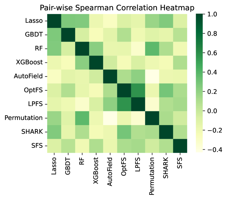
Figure 5. Similarity between feature selection methods.

In this section, we visualize the similarity between feature rankings of different feature selection methods in DRS. Figure 5 shows the heatmap of pair-wise Spearman correlation similarities. In the heatmap, the x-axis and y-axis represent different feature selection methods. The color of each square indicates the level of similarity. The more the color leans towards dark green, the more similar between the feature rankings derived from the two feature selection methods. Conversely, the more the color leans towards light green, the greater the difference in the feature rankings selected by the two methods.

We can discern the following information from the heatmap: 1) The heatmap displays three darker clusters in the upper left, middle, and lower right. This is because the features selected by the three different category methods are more similar within each category. 2) The rankings of LPFS and OptFS are highly similar. This is because they are both gate-based methods and use the L0 regularization term to control the sparsity of the gates. 3) The rankings of AutoField and Permutation are the most dissimilar. This aligns with our conclusion in Section 3.3. AutoField, as a gate-based method, determines feature importance by learning the gate weights of different feature fields during the model’s training process, aiding in uncovering features rich in information. On the other hand, Permutation, as a sensitivity-based feature selection method, judges feature importance based on the loss of effect caused by shuffling a particular feature. This approach is more conducive to identifying features with less information. Therefore, their rankings show significant differences. 4) The rankings of SHARK and SFS are quite similar because they both determine feature importance based on the gradient of the features, sharing the same source of information.

References

- (1)
- Bolón-Canedo et al. (2013) Verónica Bolón-Canedo, Noelia Sánchez-Maroño, and Amparo Alonso-Betanzos. 2013. A review of feature selection methods on synthetic data. Knowledge and information systems 34 (2013), 483–519.
- Bolón-Canedo et al. (2014) Verónica Bolón-Canedo, Noelia Sánchez-Marono, Amparo Alonso-Betanzos, José Manuel Benítez, and Francisco Herrera. 2014. A review of microarray datasets and applied feature selection methods. Information sciences 282 (2014), 111–135.
- Bommert et al. (2020) Andrea Bommert, Xudong Sun, Bernd Bischl, Jörg Rahnenführer, and Michel Lang. 2020. Benchmark for filter methods for feature selection in high-dimensional classification data. Computational Statistics & Data Analysis 143 (2020), 106839.
- Breiman (2001) Leo Breiman. 2001. Random forests. Machine learning 45 (2001), 5–32.
- Chen et al. (2022) Bo Chen, Xiangyu Zhao, Yejing Wang, Wenqi Fan, Huifeng Guo, and Ruiming Tang. 2022. A Comprehensive Survey on Automated Machine Learning for Recommendations. arXiv preprint arXiv:2204.01390 (2022).
- Chen and Guestrin (2016) Tianqi Chen and Carlos Guestrin. 2016. Xgboost: A scalable tree boosting system. In Proceedings of the 22nd acm sigkdd international conference on knowledge discovery and data mining. 785–794.
- Cheng et al. (2016) Heng-Tze Cheng, Levent Koc, Jeremiah Harmsen, Tal Shaked, Tushar Chandra, Hrishi Aradhye, Glen Anderson, Greg Corrado, Wei Chai, Mustafa Ispir, et al. 2016. Wide & deep learning for recommender systems. In Proceedings of the 1st workshop on deep learning for recommender systems. 7–10.
- Cherepanova et al. (2023) Valeriia Cherepanova, Roman Levin, Gowthami Somepalli, Jonas Geiping, C. Bruss, Andrew Wilson, Tom Goldstein, and Micah Goldblum. 2023. A Performance-Driven Benchmark for Feature Selection in Tabular Deep Learning. In NeurIPS 2023 Second Table Representation Learning Workshop.
- Darshan and Jaidhar (2018) SL Shiva Darshan and CD Jaidhar. 2018. Performance evaluation of filter-based feature selection techniques in classifying portable executable files. Procedia Computer Science 125 (2018), 346–356.
- Fan et al. (2020) Wei Fan, Kunpeng Liu, Hao Liu, Pengyang Wang, Yong Ge, and Yanjie Fu. 2020. AutoFS: Automated Feature selection via diversity-aware interactive reinforcement learning. In 2020 IEEE International Conference on Data Mining (ICDM). IEEE, 1008–1013.
- Fisher et al. (2019) Aaron Fisher, Cynthia Rudin, and Francesca Dominici. 2019. All Models are Wrong, but Many are Useful: Learning a Variable’s Importance by Studying an Entire Class of Prediction Models Simultaneously. Journal of machine learning research: JMLR 20 (2019).
- Forman (2003) George Forman. 2003. An Extensive Empirical Study of Feature Selection Metrics for Text Classification. Journal of Machine Learning Research 3 (2003), 1289–1305.
- Friedman (2001) Jerome H Friedman. 2001. Greedy function approximation: a gradient boosting machine. Annals of statistics (2001), 1189–1232.
- Granitto et al. (2006) Pablo M Granitto, Cesare Furlanello, Franco Biasioli, and Flavia Gasperi. 2006. Recursive feature elimination with random forest for PTR-MS analysis of agroindustrial products. Chemometrics and intelligent laboratory systems (2006).
- Guo et al. (2021) Huifeng Guo, Bo Chen, Ruiming Tang, Weinan Zhang, Zhenguo Li, and Xiuqiang He. 2021. An embedding learning framework for numerical features in ctr prediction. In Proceedings of the 27th ACM SIGKDD Conference on Knowledge Discovery & Data Mining. 2910–2918.
- Guo et al. (2017) Huifeng Guo, Ruiming Tang, Yunming Ye, Zhenguo Li, and Xiuqiang He. 2017. DeepFM: a factorization-machine based neural network for CTR prediction. arXiv preprint arXiv:1703.04247 (2017).
- Guo et al. (2022) Yi Guo, Zhaocheng Liu, Jianchao Tan, Chao Liao, Daqing Chang, Qiang Liu, Sen Yang, Ji Liu, Dongying Kong, Zhi Chen, et al. 2022. LPFS: Learnable Polarizing Feature Selection for Click-Through Rate Prediction. arXiv preprint arXiv:2206.00267 (2022).
- Guyon and Elisseeff (2003) Isabelle Guyon and André Elisseeff. 2003. An introduction to variable and feature selection. Journal of machine learning research 3, Mar (2003), 1157–1182.
- Heaton (2016) Jeff Heaton. 2016. An empirical analysis of feature engineering for predictive modeling. In SoutheastCon 2016. IEEE, 1–6.
- Huang et al. (2019) Tongwen Huang, Zhiqi Zhang, and Junlin Zhang. 2019. FiBiNET: combining feature importance and bilinear feature interaction for click-through rate prediction. In Proceedings of the 13th ACM Conference on Recommender Systems. 169–177.
- Lee et al. (2023) Youngjune Lee, Yeongjong Jeong, Keunchan Park, and SeongKu Kang. 2023. MvFS: Multi-view Feature Selection for Recommender System. In Proceedings of the 32nd ACM International Conference on Information and Knowledge Management. 4048–4052.
- Lin et al. (2022) Weilin Lin, Xiangyu Zhao, Yejing Wang, Tong Xu, and Xian Wu. 2022. AdaFS: Adaptive Feature Selection in Deep Recommender System. In Proceedings of the 28th ACM SIGKDD Conference on Knowledge Discovery and Data Mining (KDD). 3309–3317.
- Liu and Setiono (1995) Huan Liu and Rudy Setiono. 1995. Chi2: Feature selection and discretization of numeric attributes. In Proceedings of 7th IEEE international conference on tools with artificial intelligence. IEEE, 388–391.
- Liu et al. (2018) Hanxiao Liu, Karen Simonyan, and Yiming Yang. 2018. DARTS: Differentiable Architecture Search. In International Conference on Learning Representations.
- Liu et al. (2019) Kunpeng Liu, Yanjie Fu, Pengfei Wang, Le Wu, Rui Bo, and Xiaolin Li. 2019. Automating feature subspace exploration via multi-agent reinforcement learning. In Proceedings of the 25th ACM SIGKDD International Conference on Knowledge Discovery & Data Mining. 207–215.
- Lyu et al. (2023) Fuyuan Lyu, Xing Tang, Dugang Liu, Liang Chen, Xiuqiang He, and Xue Liu. 2023. Optimizing Feature Set for Click-Through Rate Prediction. In Proceedings of the ACM Web Conference 2023. 3386–3395.
- Ma et al. (2018) Xiao Ma, Liqin Zhao, Guan Huang, Zhi Wang, Zelin Hu, Xiaoqiang Zhu, and Kun Gai. 2018. Entire space multi-task model: An effective approach for estimating post-click conversion rate. In The 41st International ACM SIGIR Conference on Research & Development in Information Retrieval. 1137–1140.
- Rendle (2010) Steffen Rendle. 2010. Factorization Machines. In Proceedings of the 2010 IEEE International Conference on Data Mining. 995–1000.
- Rendle et al. (2009) Steffen Rendle, Christoph Freudenthaler, Zeno Gantner, and Lars Schmidt-Thieme. 2009. BPR: Bayesian personalized ranking from implicit feedback. In Proceedings of the Twenty-Fifth Conference on Uncertainty in Artificial Intelligence. 452–461.
- Shah and Kusiak (2004) Shital C Shah and Andrew Kusiak. 2004. Data mining and genetic algorithm based gene/SNP selection. Artificial intelligence in medicine 31, 3 (2004), 183–196.
- Strobl et al. (2007) Carolin Strobl, Anne-Laure Boulesteix, Achim Zeileis, and Torsten Hothorn. 2007. Bias in random forest variable importance measures: Illustrations, sources and a solution. BMC bioinformatics 8, 1 (2007), 1–21.
- Tibshirani (1996) Robert Tibshirani. 1996. Regression shrinkage and selection via the lasso. Journal of the Royal Statistical Society: Series B (Methodological) (1996).
- Vergara and Estévez (2014) Jorge R Vergara and Pablo A Estévez. 2014. A review of feature selection methods based on mutual information. Neural computing and applications 24 (2014), 175–186.
- Wang et al. (2017) Ruoxi Wang, Bin Fu, Gang Fu, and Mingliang Wang. 2017. Deep & cross network for ad click predictions. In Proceedings of the ADKDD’17. 1–7.
- Wang et al. (2023) Yejing Wang, Zhaocheng Du, Xiangyu Zhao, Bo Chen, Huifeng Guo, Ruiming Tang, and Zhenhua Dong. 2023. Single-shot Feature Selection for Multi-task Recommendations. In Proceedings of the 46th International ACM SIGIR Conference on Research and Development in Information Retrieval. 341–351.
- Wang et al. (2022) Yejing Wang, Xiangyu Zhao, Tong Xu, and Xian Wu. 2022. AutoField: Automating Feature Selection in Deep Recommender Systems. In Proceedings of the ACM Web Conference.
- Zhang et al. (2023) Beichuan Zhang, Chenggen Sun, Jianchao Tan, Xinjun Cai, Jun Zhao, Mengqi Miao, Kang Yin, Chengru Song, Na Mou, and Yang Song. 2023. SHARK: A Lightweight Model Compression Approach for Large-Scale Recommender Systems. In Proceedings of the 32nd ACM International Conference on Information and Knowledge Management (CIKM ’23).
- Zhao et al. (2020) Xiaosa Zhao, Kunpeng Liu, Wei Fan, Lu Jiang, Xiaowei Zhao, Minghao Yin, and Yanjie Fu. 2020. Simplifying reinforced feature selection via restructured choice strategy of single agent. In 2020 IEEE International Conference on Data Mining (ICDM). IEEE, 871–880.
- Zheng et al. (2023) Ruiqi Zheng, Liang Qu, Bin Cui, Yuhui Shi, and Hongzhi Yin. 2023. Automl for deep recommender systems: A survey. ACM Transactions on Information Systems 41, 4 (2023), 1–38.