Composite likelihood estimation of
stationary Gaussian processes
with a view toward stochastic volatility

Abstract

We develop a framework for composite likelihood inference of parametric continuous-time stationary Gaussian processes. We derive the asymptotic theory of the associated maximum composite likelihood estimator. We implement our approach on a pair of models that has been proposed to describe the random log-spot variance of financial asset returns. A simulation study shows that it delivers good performance in these settings and improves upon a method-of-moments estimation. In an application, we inspect the dynamic of an intraday measure of spot variance computed with high-frequency data from the cryptocurrency market. The empirical evidence supports a mechanism, where the short- and long-term correlation structure of stochastic volatility are decoupled in order to capture its properties at different time scales.

JEL Classification: C10; C80.

Keywords: Composite likelihood; stationary Gaussian processes; long memory; realized variance; roughness; stochastic volatility.

1 Introduction

The search for the most accurate description of the dynamic of time-varying volatility continues to permeate financial economics. On the one hand, it has long been recognized that realized variance is highly persistent and exhibits an autocorrelation function (acf) that perishes so slowly that it can best be approximated by a stochastic process featuring long memory (see, e.g., Andersen, Bollerslev, Diebold, and Labys, 2003; Comte and Renault, 1998; Corsi, 2009).

On the other hand, in recent years it has been suggested that the sample path of stochastic volatility may be more vibrant than implied by a standard Brownian motion. This idea was put forward by Gatheral, Jaisson, and Rosenbaum (2018), who observed that the curvature of the implied volatility surface for short-term at-the-money options is consistent with stochastic volatility being governed by a fractional Brownian motion (fBm) with a Hurst exponent less than a half. Since then, a sequence of follow-up papers studied various statistical procedures for gauging the roughness index of volatility, both under the physical and risk-neutral probability measure, largely confirming that “volatility is rough” (e.g., Bennedsen, 2020; Bolko, Christensen, Pakkanen, and Veliyev, 2023; Chong and Todorov, 2023; Wang, Xiao, and Yu, 2023).

A workhorse in this literature is the fractional Ornstein-Uhlenbeck (fOU) process, where the standard Brownian motion in the Gaussian Ornstein-Uhlenbeck process is replaced with an fBM as impetus. This model is parametric, so in principle we can do full maximum likelihood estimation (MLE) of it (Wang, Xiao, Yu, and Zhang, 2023).

In practice, MLE of the fOU process is challenging for several reasons. First, the model is generally non-Markovian. Second, in the volatility literature the state variable in the fOU represents the point-in-time log-variance of an asset price process. Previous work has employed the daily log-realized variance as an observable surrogate. However, roughness is a sample path property that concerns the behavior of a stochastic process at very short time scales. This suggests that estimation of the fOU process should be based on much more localized measure of log-variance. In this paper, we recover the log-spot variance at the intraday horizon.

However, with a long sample of a discretely observed log-spot variance process even Gaussian MLE can be prohibitive—except in special cases—because the calculation of the determinant and inversion of the covariance matrix are computationally intensive, when the number of observations is moderate-to-large, e.g. in excess of 1,000. To circumvent this issue, we propose a composite likelihood estimator for parametric stationary Gaussian processes, which nests the fOU. The composite likelihood approach—introduced in Lindsay (1988)—reduces the complexity of full MLE by only including lower-dimensional sub-models in the objective function. This effectively allows it to operate on arbitrarily large samples with minimal extra computational cost. Furthermore, while it loses asymptotic efficiency compared to MLE, in practice composite likelihood can be preferred when the full likelihood is impractical or difficult to evaluate. Moreover, in finite samples the loss of efficiency may not be too severe, since the composite likelihood function can be smoother than the full likelihood surface and, hence, much more convenient to navigate and optimize. The theoretical properties of the composite likelihood estimator have been examined in various settings, see, e.g., Cox and Reid (2004), Davis and Yau (2011) and Varin, Reid, and Firth (2011). It has also been applied to many fields, including finance (Bennedsen, Lunde, Shephard, and Veraart, 2023; Pakel, Shephard, Sheppard, and Engle, 2020).

In previous work, the fOU process has been examined with a method-of-moments estimator (MME), e.g. Bolko, Christensen, Pakkanen, and Veliyev (2023) and Wang, Xiao, and Yu (2023). The advantages of the maximum composite likelihood estimator (MCLE) over the MME are at least threefold. First, the MME for the Hurst parameter often relies on in-fill asymptotic theory to derive consistency, while our composite likelihood theory is derived within a long-span setting. The latter is appropriate, when the process is sampled discretely on a fixed equidistant partition over an expanding horizon. Second, our simulation results document that MCLE is more accurate than the MME. Thirdly, MCLE extracts the entire parameter vector in a single step rather than via a two-stage approach.

A crucial weakness of the fOU process as a model for the random log-volatility of financial asset returns is that controls both the short- and long-run persistence in a single parameter, namely the Hurst exponent. However, roughness is a sample path property of a stochastic process (leading to a rapid decline in the acf at short time scales), whereas long memory is a property of the distribution function (leading to a slow decline in the acf at long time scales). As these effects are interwined in the fOU process, it is only capable of featuring either roughness or long memory. This shortcoming was in fact highlighted by Mandelbrot (1982) in the context of the fBm. Set against this backdrop, we explore a stationary Gaussian process from a so-called Cauchy class (Gneiting and Schlather, 2004). As for the fOU process, the latter has three parameters to fit the dynamic dependence, but it reserves a separate parameter to describe the short- and long-term decay. Hence, it allows to decouple the behavior of the process at different time scales and is therefore able to account for both roughness and long memory.

The most closely related paper within the composite likelihood literature is Davis and Yau (2011). They study the theoretical properties of a pairwise likelihood estimator in a standard time series setting with discrete-time linear processes—not necessarily Gaussian—where the dependence structure is determined by the decay of the coefficients in the linear filter. By contrast, our processes evolve in continuous-time. Moreover, we develop our theory in the general framework of $q$-wise composite likelihood. Even in the pairwise setting, however, our asymptotic theory extends Davis and Yau (2011) by allowing for the presence of a slowly varying function at infinity in the autocorrelation structure of the process. This is relevant outside the fOU model, such as the Brownian semistationary process with a power kernel (e.g., Barndorff-Nielsen and Schmiegel, 2009).

In our empirical application, we inspect a vast high-frequency dataset from the cryptocurrency market. We compute a measure of spot variance based on an intraday realized variance estimator. We implement the MCLE procedure on this series in order to estimate both the fOU process and the Cauchy class. The results are striking in that the fOU, in agreement with recent work, suggests that the log-spot variance is rough, i.e. it is described by a Hurst parameter less than a half. Conversely, the Cauchy class strongly points toward a dynamic, where both roughness and long memory are required to describe the time-varying volatility. This confirm the findings from equity high-frequency data in related work of Bennedsen, Lunde, and Pakkanen (2022).

The rest of the paper is structured as follows. In Section 2, we introduce the class of stationary Gaussian processes and composite likelihood estimation. We also derive the asymptotic behaviour of the MCLE. In Section 3, we introduce the fOU process and the Cauchy class that are the concrete parametric models we investigate more in-depth. Section 4 presents a simulation study of our estimator within this framework and documents its efficacy in small samples, also compared to a MME. Section 5 contains empirical work, where we implement the technique on a high-frequency time series of log-spot variance estimates from a number of cryptocurrency spot exchange rates. In Section 6, we conclude and point to directions for further work. An appendix contains mathematical derivations.

2 Theoretical framework

In this section, we introduce the class of stationary Gaussian processes. We also present the main idea behind composite likelihood estimation. At last, we derive an asymptotic theory for parametric estimation of the former based on the latter.

2.1 Stationary Gaussian processes

In this paper, we look at processes of the form

$$Y_{t}=\mu+\nu X_{t},\quad t\in\mathbb{R},$$ (2.1)

where $\mu\in\mathbb{R}$, $\nu>0$, and $X=(X_{t})_{t\in\mathbb{R}}$ is a stationary Gaussian process with mean zero and unit variance, i.e. the marginal distribution of $X_{t}$ is standard normal. We denote the autocovariance function (acf) of $Y$ at lag $h$ as $\gamma_{h}=\text{cov}(Y_{t},Y_{t+h})=\nu^{2}E(X_{t}X_{t+h})=\nu^{2}\rho_{h}$, where $\rho_{h}$ is the acf of $X$.

Assumption 2.1.

The acf of $X$ has the property

$$\lim_{h\rightarrow\infty}\rho_{h}=0.$$ (2.2)

A stationary Gaussian process is ergodic if and only Assumption 2.1 is fulfilled (Maruyama, 1949). Since we need a law of large numbers to hold for the log-composite likelihood function, the above can therefore be viewed as a minimal regularity condition.

2.2 Composite likelihood

We suppose $\Delta>0$ is a fixed time gap and let $y=(y_{1},y_{2},\dots,y_{n})^{\top}$ be a discrete realization of $n$ equidistant observations of the random vector $(Y_{\Delta},Y_{2\Delta},\dots,Y_{n\Delta})^{\top}$, where $Y$ is the stationary continuous-time process in (2.1). We assume $\theta\in\Theta$ is a finite-dimensional parameter vector that determines the distribution of $Y$, where $\Theta\subset\mathbb{R}^{p}$ is a compact set. The data-generating value of $\theta$ is denoted $\theta_{0}$. Moreover, we initially enforce that $\mu=0$ and this is known to the econometrician. In Remark 1, we elaborate further on the effect of estimating the mean.

As the model is now parametric, we can estimate $\theta$ by maximum likelihood:

$$\hat{\theta}_{\text{MLE}}\equiv\underset{\theta\in\Theta}{\arg\max}\ l(\theta;y),$$

where $l(\theta;y)$ is the full Gaussian log-likelihood function of the sample $y$ given $\theta$, i.e.

$$l(\theta;y)\propto-\log|\Sigma_{n}|-y^{\top}\Sigma_{n}^{-1}y,$$

and $\Sigma_{n}$ is the $n\times n$ covariance matrix of $(Y_{\Delta},Y_{2\Delta},\dots,Y_{n\Delta})^{\top}$.

The maximum likelihood estimator, $\hat{\theta}_{\text{MLE}}$, is consistent, asymptotically efficient, and follows a limiting normal distribution under standard regularity conditions (e.g., Wooldridge, 1994).

However, even in the Gaussian setting, moderate values of $n$ can render numerical optimization of the log-likelihood function infeasible, because the complexity of computing the determinant and inverting the covariance matrix grows very rapidly. For example, deploying an algorithm such as the Cholesky factorization or LU decomposition results in a computational budget of $O(n^{3})$. Less naive approaches exploit the fact that the covariance matrix of a stationary process observed on an equidistant partition has a Toeplitz structure (e.g., Levinson, 1946; Durbin, 1960; Trench, 1964), yielding a faster calculation speed of $O(n^{2})$. An extra refinement has been achieved with so-called “superfast” algorithms that operate on Toeplitz matrices using the fast Fourier transform (see Brent, Gustavson, and Yun, 1980). The latter exhibit near-linear growth $O(n\log^{2}(n))$ but suffer from numerical instability in practice (see Stewart, 2003). Moreover, the scaling of these algorithms are still inferior to the linear rate $O(n)$. This poses serious issues in a high-frequency setting, where $n$ is often prohibitively large.

Set against this backdrop, we exploit the composite likelihood framework of Lindsay (1988), building on the earlier concept of pseudolikelihood from Besag (1974) in the spatial setting, see also the survey by Varin, Reid, and Firth (2011). To describe the idea, assume for the moment that $y$ is a sample of length $n$ of a continuous random variable $Y$ defined on a probability space $(\Omega,\mathcal{F},\mathbb{P})$. In general, the composite likelihood estimator maximizes a weighted product of likelihoods of marginal or conditional events. We let $f$ denote the density of $Y$ and suppose that $(\mathcal{A}_{1},\dots,\mathcal{A}_{M})$ is a collection of events, $A_{m}\in\mathcal{F}$, with likelihood $L_{m}(\theta;y)\propto f(y\in\mathcal{A}_{m};\theta)$. The composite likelihood is then defined as

$$CL(\theta;y)=\prod_{m=1}^{M}L_{m}(\theta;y)^{w_{m}},$$ (2.3)

where $w_{1},\dots,w_{M}$ are nonnegative weights with $\sum_{m}w_{m}=1$. In the remainder of the paper, we set $w_{k}=M^{-1}$ and omit it from (2.3).

The information consists of any conditional or marginal events. Hence, many variants of composite likelihood exist. Full likelihood is the special case $CL(\theta;y)=L(\theta;y)=f(y;\theta)$. The independence likelihood is $CL(\theta;y)=\prod_{i=1}^{n}f(y_{i};\theta)$. It permits inference on marginal parameters only and is the full likelihood under actual independence. However, it is necessary to add events formed from blocks of observations to estimate parameters that control the dependence structure, such as the pairwise likelihood of Cox and Reid (2004), $CL(\theta;y)=\prod_{i=1}^{n}\prod_{j=i+1}^{n}f(y_{i},y_{j};\theta)$, or the restricted version named consecutive pairwise likelihood by Davis and Yau (2011), $CL(\theta;y)=\prod_{i=1}^{n-K}\prod_{j=i}^{i+K}f(y_{i},y_{j};\theta)$, which includes neighboring pairs up to some order $K\in\mathbb{N}$ with $K<n$. Another candidate is the conditional likelihood $CL(\theta;y)=\prod_{i=1}^{n}f(y_{i}\mid y\setminus y_{i};\theta)$.

The maximum composite likelihood estimator (MCLE) is the argmax of $CL(\theta;y)$—or the natural logarithm of it:

$$\hat{\theta}_{\mathrm{MCLE}}\equiv\underset{\theta\in\Theta}{\arg\max}\ cl(\theta;y),$$

where

$$cl(\theta;y)=\log CL(\theta;y)=\sum_{m=1}^{M}\log L_{m}(\theta;y).$$

The composite log-likelihood function is, in general, not proportional to the full likelihood (and therefore not always a genuine likelihood), so the model is misspecified (see, e.g., White, 1982). However, this is not an example, where the data-generating probability measure is completely unrelated to the assumed parametric distribution. Here, the marginal (or conditional) densities included in (2.4) are extracted from the true model and correctly specified. Hence, the score of $cl(\theta;y)$ satisfies the first Bartlett identity and forms a collection of unbiased estimating equations. As we show below, it follows by a law of large numbers that $\hat{\theta}_{\mathrm{MCLE}}$ is consistent for the true parameter value, $\theta_{0}$, rather than some pseudo-parameter minimizing the Kullback-Leibler divergence between the true and assumed model. Moreover, if the memory in the process is not too strong, $\hat{\theta}_{\mathrm{MCLE}}$ is also asymptotically normal.

2.3 Asymptotic theory

In the present paper, we establish an asymptotic theory for a $q$-wise composite likelihood estimator, where the composite likelihood function is formed as an equal weighted product of marginal events defined via the selection of tuples of up to length $q$. It nests both the independence likelihood and the pairwise likelihood as special cases. We take $K\in\mathbb{N}$ fixed and let $Q$ be a collection of $K$ $q^{j}$-tuples of natural numbers, where $q^{j}\in\mathbb{N}$, i.e. tuples of the form $k^{j}=(0,k_{2}^{j},\dots,k_{q^{j}}^{j})\in\{0\}\times\mathbb{N}^{q^{j}-1}$ for $j=1,\dots,K$, indexing which observations to add. Here, we use the convention that $\mathbb{N}^{0}=\emptyset$. To ease notation, we set $q=\max_{j=1,\dots,K}q^{j}$. Moreover, we suppose without loss of generality that the indices are increasing and that $\max_{j=1,\dots,K}k_{q^{j}}^{j}<n$. For $k^{j}\in Q$, we let $f_{k^{j}}(y_{i}^{k^{j}};\theta)=f_{k^{j}}(y_{i},y_{i+k_{2}^{j}},\dots,y_{i+k_{q^{j}}^{j}};\theta)$ denote the density of $Y_{i}^{k^{j}}=(Y_{i},Y_{i+k_{2}^{j}},\dots,Y_{i+k_{q^{j}}^{j}})$, which by stationary is independent of $i$.

The $q$-wise log-composite likelihood can be written

$$cl(\theta;y)=\sum_{k^{j}\in Q}\sum_{i=1}^{n-k^{j}_{q^{j}}}\log f_{k^{j}}(y_{i}^{k^{j}};\theta).$$ (2.4)

To prove our asymptotic theory, we need a identification assumption to ensure that the log-composite likelihood is uniquely maximized at $\theta_{0}$:

Assumption 2.2.

We assume that for any $\theta\in\Theta$ with $\theta\neq\theta_{0}:\sum_{k^{j}\in Q}f_{k^{j}}(y^{k^{j}},\theta)\neq\sum_{k^{j}\in Q}f_{k^{j}}(y^{k^{j}},\theta_{0})$ for a set of vectors $y\in\mathbb{R}^{q}$ of non-zero measure.

Assumption 2.2, together with the moment condition $E(|\log f(y;\theta)|)<\infty$, are sufficient to ensure a unique maximum at $\theta_{0}$ by the information inequality, see Newey and McFadden (1994, Lemma 2.2). The existence of the moment holds trivially for the Gaussian distribution. Moreover, in our setting the assumption can be verified if $K$ and $q$ are sufficiently large relative to the dimension of $\theta$, $p$. Of course, this assumes that all the parameters of the model enter into the densities of the chosen events in $Q$, and that they do so in a way that is linearly independent.

Our first result is a law of large numbers.

Theorem 2.1.

Assume that the true model is the stationary Gaussian process defined in (2.1) and that Assumptions 2.1 – 2.2 hold. Then, as $n\rightarrow\infty$,

$$\hat{\theta}_{\mathrm{MCLE}}\overset{\mathbb{P}}{\longrightarrow}\theta_{0}.$$

The proofs of our results are presented in Appendix A.

Next, we derive the asymptotic distribution of our estimator. The theorem consists of several parts, because both the rate of convergence of $\hat{\theta}_{\mathrm{MCLE}}$ and the shape of the limiting distribution of the estimation error depends on the persistence of the process.

Theorem 2.2.

Suppose the conditions from Theorem 2.1 hold and that $\theta_{0}$ is an interior point, i.e. $\theta_{0}\in\mathrm{int}(\Theta)$. Let $L_{\infty}$ be a slowly varying function at infinity, i.e. $\lim_{x\rightarrow\infty}L_{\infty}(tx)\div L_{\infty}(x)=1$, for all $t>0$. Then, as $n\rightarrow\infty$, it holds that

1. If $\int_{0}^{\infty}\gamma_{h}\mathrm{d}h<\infty$ or if $\gamma_{h}\sim h^{-\beta}L_{\infty}(h)$ as $h\rightarrow\infty$ for $\beta\in(1/2,1)$, then

   $$\sqrt{n}\big{(}\hat{\theta}_{\mathrm{MCLE}}-\theta_{0}\big{)}\overset{d}{\longrightarrow}N\left(0,G(\theta_{0})^{-1}\right),$$

   with

   $$G(\theta_{0})^{-1}=H(\theta_{0})^{-1}V(\theta_{0})H(\theta_{0})^{-1},$$

   $$H(\theta_{0})=-\sum_{k\in Q}\mathbb{E}\left(\frac{\partial^{2}}{\partial\theta^{\top}\partial\theta}\log\left(f_{k}(Y_{k};\theta)\right)\mid_{\theta=\theta_{0}}\right),$$

   and

   $$V(\theta_{0}) =\lim_{n\rightarrow\infty}\frac{1}{n}\mathbb{E}\left(s_{n}(\theta)s_{n}(\theta)^{\top}\right)$$

   $$=\frac{1}{4}\sum_{k^{1},k^{2}\in Q}\sum_{l=-\infty}^{\infty}\sum_{j_{1},j_{2}\in k_{1}}\sum_{j_{3},j_{4}\in k_{2}}\left[\frac{\partial}{\partial\theta_{r}}\big{(}\Sigma_{k^{1}}^{-1}(\theta)\big{)}_{j_{1},j_{2}}\right]_{r=1}^{p}$$

   $$\times\left(\left[\frac{\partial}{\partial\theta_{r}}\big{(}\Sigma_{k^{1}}^{-1}(\theta)\big{)}_{j_{3},j_{4}}\right]_{r=1}^{p}\right)^{\top}\times\left(\gamma_{l+j_{1}-j_{3}}\gamma_{l+j_{2}-j_{4}}+\gamma_{l+j_{1}-j_{4}}\gamma_{l+j_{2}-j_{3}}\right),$$

   where $s_{n}(\theta)=\frac{\partial}{\partial\theta}cl(\theta;y)$. Furthermore, the infinite series defining $V(\theta_{0})$ is convergent.

2. If $\gamma_{h}\sim h^{-1/2}L_{\infty}(h)$ as $h\rightarrow\infty$, then

   $$\frac{\sqrt{n}}{\sqrt{L_{\gamma}(n)}}\big{(}\hat{\theta}_{\mathrm{MCLE}}-\theta_{0}\big{)}\overset{d}{\longrightarrow}N\left(0,G(\theta_{0})^{-1}\right),$$

   with $G(\theta_{0})$ and $H(\theta_{0})$ defined as above, but where the variability matrix is redefined as

   $$V(\theta_{0}) =\lim_{n\rightarrow\infty}\frac{1}{nL_{\gamma}(n)}\mathbb{E}\left(s_{n}(\theta)s_{n}(\theta)^{\top}\right)$$

   $$=\lim_{n\rightarrow\infty}\frac{1}{4}\frac{1}{L_{\gamma}(n)}\sum_{k^{1},k^{2}\in Q}\sum_{l=-n}^{n}\sum_{j_{1},j_{2}\in k_{1}}\sum_{j_{3},j_{4}\in k_{2}}\left[\frac{\partial}{\partial\theta_{r}}\big{(}\Sigma_{k^{1}}^{-1}(\theta)\big{)}_{j_{1},j_{2}}\right]_{r=1}^{p}$$

   $$\times\left(\left[\frac{\partial}{\partial\theta_{r}}\big{(}\Sigma_{k^{2}}^{-1}(\theta)\big{)}_{j_{3},j_{4}}\right]_{r=1}^{p}\right)^{\top}\times\left(\gamma_{l+j_{1}-j_{3}}\gamma_{l+j_{2}-j_{4}}+\gamma_{l+j_{1}-j_{4}}\gamma_{l+j_{2}-j_{3}}\right),$$

   and $L_{\gamma}$ is a slowly varying function, related to $L_{\infty}$, as defined in Appendix A.

3. If $\gamma_{h}\sim h^{-\beta}L_{\infty}(h)$ as $h\rightarrow\infty$ for $\beta\in(0,1/2)$, then

   $$n^{\beta}L_{2}^{-1/2}(n)(\hat{\theta}_{\mathrm{MCLE}}-\theta_{0})\overset{d}{\longrightarrow}H(\theta_{0})^{-1}\Psi Z_{2,H}(1),$$ (2.5)

   where $L_{2}(n)=2C_{2}L^{2}_{\infty}(n)$, $C_{2}=[(1-2\beta)(2-\beta)]^{-1}$, $\Psi$ is a $p\times 1$ vector with elements

   $$\Psi_{r}=\frac{1}{2}\sum_{k^{j}\in Q}\sum_{j_{1},j_{2}\in k^{j}}\frac{\partial}{\partial\theta_{r}}\big{(}\Sigma_{k}^{-1}(\theta)\big{)}_{j_{1},j_{2}},$$ (2.6)

   for $r=1,\dots,p$ and $Z_{2,H}$ is a Rosenblatt process with parameter $1-\beta/2$.

The first part covers the short memory setting with an integrable acf, but it also permits long memory (as defined in (3.2)) with $\beta\in(1/2,1)$. Here, we get a standard central limit theorem with a standard $n^{-1/2}$ rate of convergence. However, because the composite likelihood misspecifies the true likelihood, the second Bartlett identity (or information matrix equality) is violated, so the Fisher information is replaced with the Godambe (1960) information, which has a sandwich form. The ratio of these matrices determines the loss of efficiency of $\hat{\theta}_{\text{MCLE}}$ relative to $\hat{\theta}_{\text{MLE}}$, which achieves the Cramer-Rao lower bound asymptotically. This is the price we pay for not doing full maximum likelihood.

The second part is the borderline case with $\beta=1/2$, where the polynomial decay in the long memory setting starts to impair the convergence toward the asymptotic distribution of $\hat{\theta}_{\mathrm{MCLE}}$. Here, the variability matrix has to be scaled by an additional term, $L_{\gamma}(n)$, whereby the overall rate of convergence is reduced, but the limit remains Gaussian. An inspection of the expression for $L_{\gamma}(n)$ in Appendix A shows that, even if $\lim_{h\rightarrow\infty}L_{\infty}(h)$ exists, the convergence rate of $\hat{\theta}_{\text{MCLE}}$ deteriorates to $\log(n)n^{-1/2}$, as consistent with Davis and Yau (2011).

In the last part, $\beta\in(0,1/2)$, so the acf subsides exceedingly slow. Here, we get a non-central limit theorem with a non-standard convergence rate, which is nevertheless a classical result in the realm of long memory processes.

In practice, the variance-covariance matrix of the composite score function in the limiting distribution, $V(\theta_{0})$, of $\hat{\theta}_{\text{MCLE}}$ is challenging to compute, since the gradient vanishes at $\theta=\hat{\theta}_{\text{MCLE}}$. Instead, we propose to estimate $G^{-1}(\theta_{0})$ via a parametric bootstrap.

Our analysis extends Davis and Yau (2011) from pairwise likelihood to the $q$-wise setting. However, even with $q=2$ we allow for the presence of a slowly varying function in the acf, which is important for some Gaussian processes, such as the Brownian semistationary process with a power law kernel (e.g. Bennedsen, Lunde, and Pakkanen, 2022).

Remark 1.

In the above, $\mu=0$ is known to hold. It is of course straightforward to transform a problem with a known nonzero mean into the previous setting by appropriate centering. What if the mean is unknown and, hence, estimated?

The composite likelihood estimator is derived from the score of the log-composite likelihood function, and since we work with Gaussian data, the stochastic terms in the score relate to the autocovariance function of the process. Hence, the main difference between these settings corresponds to the limit theory for autocovariances calculated with a known mean or estimated mean. This was analyzed in the Gaussian setting by Hosking (1996), who shows that if the memory is not too strong (i.e. short memory or long memory with $\beta>1/2$), there is no impact. That is, estimating the mean does not alter neither the rate of convergence nor the limiting distribution.

On the other hand, with pervasive long memory (i.e. $\beta<1/2$), estimation of the mean makes a difference relative to our case 3. While the convergence rate is unchanged, the limiting distribution is no longer a Rosenblatt distribution, but it has a more complicated expression. It also instills an important finite sample downward bias in the sample acf, which impairs the estimation in practice. We shed light on this in the simulation study.

3 A view toward stochastic volatility

In this section, we narrow down the estimation of continuous-time stationary Gaussian processes to a particular pair of parametric models. The first is the fractional Ornstein-Uhlenbeck process (fOU), which has attracted a lot of attention in the recent literature on roughness in the stochastic volatility of financial asset returns (e.g., Gatheral, Jaisson, and Rosenbaum, 2018; Fukasawa, Takabatake, and Westphal, 2022; Bolko, Christensen, Pakkanen, and Veliyev, 2023; Wang, Xiao, and Yu, 2023). The second is from a so-called Cauchy class, which was proposed in Gneiting and Schlather (2004). In financial econometrics, it has—to the best of our knowledge—only been studied as a volatility model by Bennedsen, Lunde, and Pakkanen (2022).

We begin with a notion of roughness and memory.

Definition 1.

A stationary stochastic process has roughness index $\alpha$ if its acf has the following behaviour around the origin:

$$(1-\rho(h))\sim L(h)|h|^{2\alpha+1},\quad|h|\rightarrow 0,$$ (3.1)

for a function $L(h)$ that is slowly varying at zero and $\alpha\in(-1/2,1/2)$.

A Brownian motion has $\alpha=0$. Moreover, because it is a continuous Gaussian process, there is a one-to-one correspondence between the roughness index and the Hölder continuity of its sample paths (Bennedsen, 2020). Thus, we refer to a process as being rough if it has a negative roughness index, $\alpha<0$, as its sample paths are then more irregular—i.e. less Hölder continuous—than those of a Brownian motion. Conversely, we call a process smooth if it has a positive roughness index, $\alpha>0$.

Definition 2.

A stationary stochastic process has long memory of degree $\beta$ if its acf decays at a polynomial rate as the lag length increases:

$$\rho(h)\sim L_{\infty}(h)|h|^{-\beta},\quad|h|\rightarrow\infty,$$ (3.2)

for some function, $L_{\infty}(h)$, that is slowly varying at infinity, and $\beta\in(0,1]$.

The requirement on $\beta$ implies that the acf is not integrable, which is another common way to define long memory in a time series. Here, we stick to Definition 2, which suffices for the purposes of this paper. If the acf is integrable, we say the process has short memory, even if it is does not vanish at an exponential rate.

3.1 The fOU process

The first class of parametric stationary Gaussian processes that we entertain in this paper is the fOU process:

$$\mathrm{d}Y_{t}=-\kappa(Y_{t}-\mu)\mathrm{d}t+\nu\mathrm{d}B_{t}^{H},$$ (3.3)

where $B^{H}$ is a fractional Brownian motion (fBm).

The unique stationary solution to this stochastic differential equation was derived in Cheridito, Kawaguchi, and Maejima (2003):

$$Y_{t}=\mu+\nu X_{t},$$ (3.4)

where $X_{t}=\sqrt{\dfrac{\kappa^{2H}}{H\Gamma(2H)}}\int_{-\infty}^{t}e^{-\kappa(t-s)}\mathrm{d}B_{s}^{H}$ and $\Gamma$ is the Gamma function. The additional scaling in front of the stochastic integral in (3.4) relative to (3.3) is a reparameterization of the model to ensure $\nu$ can be interpreted as the standard deviation of $Y_{t}$. It follows from $\text{var}\left(\int_{-\infty}^{t}e^{-\kappa(t-s)}\mathrm{d}B_{s}^{H}\right)=\kappa^{-2H}H\Gamma(2H)$.

The acf of the fOU is available from Garnier and Sølna (2018):

$$\begin{split}\rho_{h}=\frac{1}{2\kappa^{2H}}\left(\frac{1}{2}\int_{-\infty}^{\infty}e^{-|y|}|\kappa h+y|^{2H}\mathrm{d}y-|\kappa h|^{2H}\right).\end{split}$$ (3.5)

The acf of the fBm decays hyperbolically with $\rho_{h}=O(h^{2(H-1)})$ for $H\neq 1/2$, whereas for $H=1/2$ it is geometrically bounded. Moreover, it follows from Cheridito, Kawaguchi, and Maejima (2003) that the acf of the fOU process inherits the order of decay of the background driving fBm.

By the Kolmogorov-Chentsov theorem (Chentsov, 1956), fBm has a modification, where the sample paths are Hölder continuous with exponent $\gamma\in(0,H)$. So the Hurst parameter determine how regular the paths are and it is linked to the roughness index in (3.1) through the relation $\alpha=H-1/2$. Hence, for $H<1/2$ the fBm process is rough, whereas for $H>1/2$ it is smooth. Furthermore, it readily follows that it has long memory for $H>1/2$, whereas it is possesses short memory for $H\leq 1/2$. As before, these properties are passed down to the fOU process.

This bottom line is that the Hurst exponent controls both the roughness and memory properties of the fOU process. This renders it capable of exhibiting either roughness or long memory, but not both. This is also rather intuitive, since an examination of the acf of the time-changed process $B_{ct}^{H}$, for some $c>0$, reveals that the fBm is self-similar.

3.2 The Cauchy class

There is, to the best of our knowledge, no known representation of these processes in the form of a stochastic differential equation describing their dynamic. Hence, the Cauchy class is solely defined via the correlation structure:

$$\rho_{h}=(1+|h|^{2\alpha+1})^{-\beta/(2\alpha+1)}$$ (3.6)

for $\alpha\in(-1/2,1/2)$ and $\beta>0$. It follows that $\rho_{h}$ behaves as (3.1) for $h\rightarrow 0$ and as (3.2) for $h\rightarrow\infty$.

The Cauchy class can also exhibit roughness and long memory. However, whereas these properties are forged together by the Hurst exponent for the fOU process, here the features are decoupled and controlled by separate parameters, $\alpha$ and $\beta$, such that it can exhibit both roughness ($\alpha<0$) and long memory ($\beta<1$).

Motivated by its ability to decouple the short- and long-term persistence, this process was studied as a empirical model for log-spot variance in Bennedsen, Lunde, and Pakkanen (2022). They fitted it with method of moments to high-frequency data from the E-mini S&P 500 futures contract and indeed found evidence of both roughness and long memory.

4 Monte Carlo simulation

To inspect the small sample properties of our CLE procedure, we simulate the stationary Gaussian processes from Section 3, i.e. the fOU process and Cauchy class. The parameter vector is four-dimensional, i.e. $\theta_{\text{OU}}=(\mu,\kappa,\nu,\alpha)^{\top}$ and $\theta_{\text{CC}}=(\mu,\beta,\nu,\alpha)^{\top}$. To shed light on the importance of Remark 1, we fix $\mu=0$ and examine the impact of knowing this a priori, so $\mu$ is not estimated, and the setup where $\mu$ is inferred alongside the covariance-related parameters.

The fOU model was studied in Bolko, Christensen, Pakkanen, and Veliyev (2023) and Wang, Xiao, and Yu (2023) to describe the stochastic log-variance of financial asset returns, $Y_{t}=\log\sigma_{t}^{2}$. We follow this analogue here and adopt the Monte Carlo design of the former article by examining five different settings for $\theta_{\text{OU}}$ (listed in Table 1) ranging from very rough and short memory ($\alpha=-0.45$ or $H=0.05$) to smooth and long memory ($\alpha=0.20$ or $H=0.70$). We include an equal number of distinct parameter values for $\theta_{\text{CC}}$ (listed in Table 3), keeping the roughness index fixed at the values of the Hurst exponent from the fOU process, i.e. $\alpha=-0.45,-0.40,\dots,0.20$, while moving the long-run persistence in the opposite direction, i.e. $\beta=0.25,0.50,\dots,1.25$. This design ensures that the latter features multiple settings with both roughness and long memory.

We simulate over the interval $[0,T]$, where $T$ can be interpreted as the number of days, setting $T=1095,1825,2555$. This amounts to three, five, and seven years worth of data. The intermediate value roughly matches the sample size in our empirical application. We assume the process is observed discretely on an equispaced partition of $N$ points per day, so the $n=N\times T+1$ data vector is $(Y_{t-1+i\Delta})_{t=1,\dots,T\text{ and }i=0,1,\dots,N}$, where $\Delta=1/N$. We follow Christensen, Thyrsgaard, and Veliyev (2019) and Li, Todorov, and Tauchen (2013) and base the analysis on $N=12$ observations per unit interval, yielding a new observation of the log-spot variance every second hour.

We simulate the Cauchy class via circulant embedding (e.g., Asmussen and Glynn, 2007), which is an exact discretization that runs in $O(n\log n)$ time. However, since the acf of the fOU needs to be evaluated with the help of numerical integration we opt for a slightly different approach for that model. In particular, at a generic time $t$, the solution of the fOU process in (3.4) implies that:

$$Y_{t}=\mu+(Y_{t-\Delta}-\mu)e^{-\kappa\Delta}+\nu\sqrt{\dfrac{\kappa^{2H}}{H\Gamma(2H)}}\int_{t-\Delta}^{t}e^{-\kappa(t-s)}\text{d}B_{s}^{H}.$$

We approximate the stochastic integral as $\int_{t-\Delta}^{t}e^{-\kappa(t-s)}\text{d}B_{s}^{H}\simeq e^{-\kappa\Delta/2}(B_{t}^{H}-B_{t-\Delta}^{H})$ and simulate increments of the fBm with circulant embedding.

To implement CL, we need to decide the terms to include in (2.4) through the set $Q$. We experiment with triwise (i.e. $q^{j}=q=3$) CLE with $K=18$, where the elements of $k^{j}$ are separated by a fixed amount, i.e. $k^{j}=(0,\ell,2\ell)$ for $\ell=1,\dots,10$, 50, 100, 200, 500, 1000, 2000, 5000, 10000. This setup means that $cl(\theta;y)$ is a summation of densities of the form $f(y_{i},y_{i+\ell},y_{i+2\ell};\theta)$. The reported results are rather robust to the exact configuration of the CL procedure.

We benchmark MCLE against a method-of-moments estimator (MME). We follow the implementation of Wang, Xiao, and Yu (2023) for the fOU process and Bennedsen, Lunde, and Pakkanen (2022) for the Cauchy class. The details are reviewed in Appendix B. It is worth pointing out that the first-step MME estimator of $\alpha$ (or $H$) relies on change-of-frequency approach based on first-differenced data. Hence, it does not depend on whether the mean is known or estimated. We should also emphasize that we start the MCLE routine with the MME as initial value.

In the left-hand side of Table 1 – 2, we report the Monte Carlo average (standard error in parenthesis) of each parameter estimate for the fOU process, while Table 3 – 4 presents the corresponding results for the Cauchy class. The MME is shown in the right-hand side of each table. The number of Monte Carlo replications is 10,000.

Table 1: Parameter estimation of the fOU process ($\mu$ known).

Parameter	Value	MCLE				MME
		$T=1{,}095$	$T=1{,}825$	$T=2{,}555$		$T=1{,}095$	$T=1{,}825$	$T=2{,}555$
Panel A:
$\mu$	0.000	0.0000 (0.0000)	0.0000 (0.0000)	0.0000 (0.0000)		0.0000 (0.0000)	0.0000 (0.0000)	0.0000 (0.0000)
$\kappa$	0.005	0.0057 (0.0066)	0.0052 (0.0048)	0.0052 (0.0039)		0.0106 (0.0199)	0.0085 (0.0132)	0.0075 (0.0102)
$\nu$	1.250	1.2339 (0.4392)	1.2515 (0.0089)	1.2499 (0.0064)		1.2500 (0.0406)	1.2500 (0.0318)	1.2500 (0.0270)
$\alpha$	-0.450	-0.4514 (0.0069)	-0.4489 (0.0056)	-0.4491 (0.0045)		-0.4502 (0.0133)	-0.4501 (0.0104)	-0.4501 (0.0088)
Panel B:
$\mu$	0.000	0.0000 (0.0000)	0.0000 (0.0000)	0.0000 (0.0000)		0.0000 (0.0000)	0.0000 (0.0000)	0.0000 (0.0000)
$\kappa$	0.010	0.0121 (0.0063)	0.0109 (0.0045)	0.0107 (0.0037)		0.0140 (0.0141)	0.0124 (0.0100)	0.0118 (0.0080)
$\nu$	0.750	0.7405 (0.0069)	0.7505 (0.0053)	0.7502 (0.0045)		0.7500 (0.0244)	0.7500 (0.0191)	0.7500 (0.0162)
$\alpha$	-0.400	-0.4039 (0.0083)	-0.3993 (0.0067)	-0.3995 (0.0056)		-0.4002 (0.0131)	-0.4001 (0.0103)	-0.4001 (0.0087)
Panel C:
$\mu$	0.000	0.0000 (0.0000)	0.0000 (0.0000)	0.0000 (0.0000)		0.0000 (0.0000)	0.0000 (0.0000)	0.0000 (0.0000)
$\kappa$	0.015	0.0185 (0.0072)	0.0162 (0.0049)	0.0159 (0.0041)		0.0171 (0.0080)	0.0162 (0.0060)	0.0159 (0.0049)
$\nu$	0.500	0.4980 (0.0083)	0.5004 (0.0065)	0.5003 (0.0055)		0.5000 (0.0164)	0.5000 (0.0128)	0.5000 (0.0108)
$\alpha$	-0.200	-0.2034 (0.0155)	-0.1994 (0.0121)	-0.1995 (0.0102)		-0.2002 (0.0125)	-0.2002 (0.0097)	-0.2001 (0.0082)
Panel D:
$\mu$	0.000	0.0000 (0.0000)	0.0000 (0.0000)	0.0000 (0.0000)		0.0000 (0.0000)	0.0000 (0.0000)	0.0000 (0.0000)
$\kappa$	0.035	0.0408 (0.0114)	0.0364 (0.0080)	0.0361 (0.0067)		0.0371 (0.0102)	0.0362 (0.0078)	0.0359 (0.0065)
$\nu$	0.300	0.2999 (0.0076)	0.3003 (0.0059)	0.3002 (0.0049)		0.3000 (0.0103)	0.3000 (0.0080)	0.3000 (0.0068)
$\alpha$	0.000	-0.0014 (0.0171)	0.0001 (0.0132)	0.0002 (0.0110)		-0.0001 (0.0117)	-0.0002 (0.0091)	-0.0001 (0.0077)
Panel E:
$\mu$	0.000	0.0000 (0.0000)	0.0000 (0.0000)	0.0000 (0.0000)		0.0000 (0.0000)	0.0000 (0.0000)	0.0000 (0.0000)
$\kappa$	0.070	0.0823 (0.0319)	0.0726 (0.0180)	0.0718 (0.0138)		0.0732 (0.0157)	0.0720 (0.0122)	0.0715 (0.0103)
$\nu$	0.200	0.2032 (0.0245)	0.2008 (0.0129)	0.2004 (0.0096)		0.2000 (0.0079)	0.2000 (0.0061)	0.2000 (0.0052)
$\alpha$	0.200	0.2015 (0.0276)	0.1995 (0.0187)	0.1995 (0.0146)		0.1998 (0.0109)	0.1998 (0.0085)	0.1999 (0.0071)

Note. We simulate the process in the caption of the table 10,000 times on the interval $[0,T]$, where $T$ is interpreted as the number of days. There are $N=12$ observations per unit interval, corresponding to an observation every second hour. The true value of the parameter vector appear to the left in Panel A – E. We estimate $\theta$ with the maximum composite likelihod estimation (MCLE) procedure developed in the main text, and benchmark it against a method-of-moments estimator (MME). The table reports the Monte Carlo average value of each parameter estimate across simulations (standard deviation in parenthesis).

Table 2: Parameter estimation of the fOU process ($\mu$ estimated).

Parameter	Value	MCLE				MME
		$T=1{,}095$	$T=1{,}825$	$T=2{,}555$		$T=1{,}095$	$T=1{,}825$	$T=2{,}555$
Panel A:
$\mu$	0.000	-0.0007 (0.3250)	0.0013 (0.2053)	0.0005 (0.1461)		-0.0005 (0.2582)	0.0005 (0.1647)	0.0001 (0.1208)
$\kappa$	0.005	0.0077 (0.0075)	0.0059 (0.0047)	0.0057 (0.0039)		0.0132 (0.0232)	0.0094 (0.0143)	0.0080 (0.0107)
$\nu$	1.250	1.2326 (0.2323)	1.2515 (0.0281)	1.2503 (0.0168)		1.2500 (0.0406)	1.2500 (0.0318)	1.2500 (0.0270)
$\alpha$	-0.450	-0.4506 (0.0065)	-0.4488 (0.0054)	-0.4491 (0.0045)		-0.4502 (0.0133)	-0.4501 (0.0104)	-0.4501 (0.0088)
Panel B:
$\mu$	0.000	-0.0003 (0.0933)	0.0002 (0.0632)	0.0000 (0.0452)		-0.0004 (0.0936)	0.0001 (0.0622)	-0.0001 (0.0467)
$\kappa$	0.010	0.0133 (0.0067)	0.0114 (0.0047)	0.0110 (0.0038)		0.0150 (0.0150)	0.0128 (0.0103)	0.0120 (0.0082)
$\nu$	0.750	0.7405 (0.0069)	0.7505 (0.0054)	0.7502 (0.0045)		0.7500 (0.0244)	0.7500 (0.0191)	0.7500 (0.0162)
$\alpha$	-0.400	-0.4034 (0.0080)	-0.3992 (0.0066)	-0.3994 (0.0055)		-0.4002 (0.0131)	-0.4001 (0.0103)	-0.4001 (0.0087)
Panel C:
$\mu$	0.000	-0.0004 (0.0978)	0.0002 (0.0708)	-0.0000 (0.0556)		-0.0004 (0.0972)	0.0001 (0.0699)	-0.0001 (0.0556)
$\kappa$	0.015	0.0203 (0.0076)	0.0170 (0.0051)	0.0164 (0.0042)		0.0182 (0.0086)	0.0168 (0.0062)	0.0163 (0.0050)
$\nu$	0.500	0.4986 (0.0082)	0.5007 (0.0065)	0.5005 (0.0054)		0.5000 (0.0164)	0.5000 (0.0128)	0.5000 (0.0108)
$\alpha$	-0.200	-0.2018 (0.0149)	-0.1987 (0.0119)	-0.1990 (0.0101)		-0.2002 (0.0125)	-0.2002 (0.0097)	-0.2001 (0.0082)
Panel D:
$\mu$	0.000	-0.0001 (0.0682)	0.0002 (0.0533)	0.0000 (0.0450)		-0.0001 (0.0677)	0.0002 (0.0528)	-0.0000 (0.0447)
$\kappa$	0.035	0.0438 (0.0117)	0.0381 (0.0082)	0.0372 (0.0068)		0.0390 (0.0107)	0.0374 (0.0080)	0.0367 (0.0066)
$\nu$	0.300	0.3009 (0.0075)	0.3009 (0.0058)	0.3006 (0.0049)		0.3000 (0.0103)	0.3000 (0.0080)	0.3000 (0.0068)
$\alpha$	0.000	0.0005 (0.0163)	0.0012 (0.0129)	0.0010 (0.0108)		-0.0001 (0.0117)	-0.0002 (0.0091)	-0.0001 (0.0077)
Panel E:
$\mu$	0.000	0.0003 (0.0691)	0.0002 (0.0591)	0.0001 (0.0538)		0.0003 (0.0688)	0.0002 (0.0589)	0.0001 (0.0534)
$\kappa$	0.070	0.0837 (0.0177)	0.0745 (0.0130)	0.0735 (0.0109)		0.0795 (0.0158)	0.0765 (0.0120)	0.0752 (0.0101)
$\nu$	0.200	0.2007 (0.0073)	0.1999 (0.0058)	0.1999 (0.0049)		0.2000 (0.0079)	0.2000 (0.0061)	0.2000 (0.0052)
$\alpha$	0.200	0.1937 (0.0146)	0.1945 (0.0123)	0.1955 (0.0101)		0.1998 (0.0109)	0.1998 (0.0085)	0.1999 (0.0071)

Note. We simulate the process in the caption of the table 10,000 times on the interval $[0,T]$, where $T$ is interpreted as the number of days. There are $N=12$ observations per unit interval, corresponding to an observation every second hour. The true value of the parameter vector appear to the left in Panel A – E. We estimate $\theta$ with the maximum composite likelihod estimation (MCLE) procedure developed in the main text, and benchmark it against a method-of-moments estimator (MME). The table reports the Monte Carlo average value of each parameter estimate across simulations (standard deviation in parenthesis).

Table 3: Parameter estimation of the Cauchy class ($\mu$ known).

Parameter	Value	MCLE				MME
		$T=1{,}095$	$T=1{,}825$	$T=2{,}555$		$T=1{,}095$	$T=1{,}825$	$T=2{,}555$
Panel A:
$\mu$	0.000	0.0000 (0.0000)	0.0000 (0.0000)	0.0000 (0.0000)		0.0000 (0.0000)	0.0000 (0.0000)	0.0000 (0.0000)
$\beta$	0.250	0.3256 (0.2026)	0.3469 (0.1611)	0.3387 (0.1508)		0.1718 (0.0980)	0.1537 (0.0814)	0.1446 (0.0714)
$\nu$	1.250	1.2129 (0.0701)	1.2492 (0.0666)	1.2491 (0.0629)		1.2489 (0.0720)	1.2491 (0.0666)	1.2491 (0.0628)
$\alpha$	-0.450	-0.4478 (0.0270)	-0.4395 (0.0188)	-0.4403 (0.0176)		-0.4807 (0.0100)	-0.4817 (0.0081)	-0.4822 (0.0072)
Panel B:
$\mu$	0.000	0.0000 (0.0000)	0.0000 (0.0000)	0.0000 (0.0000)		0.0000 (0.0000)	0.0000 (0.0000)	0.0000 (0.0000)
$\beta$	0.500	0.5437 (0.1704)	0.5398 (0.1397)	0.5336 (0.1271)		0.3521 (0.1207)	0.3392 (0.1020)	0.3317 (0.0904)
$\nu$	0.750	0.7278 (0.0202)	0.7501 (0.0179)	0.7500 (0.0158)		0.7500 (0.0211)	0.7501 (0.0178)	0.7500 (0.0157)
$\alpha$	-0.400	-0.4000 (0.0220)	-0.3960 (0.0174)	-0.3966 (0.0159)		-0.4594 (0.0134)	-0.4594 (0.0104)	-0.4593 (0.0088)
Panel C:
$\mu$	0.000	0.0000 (0.0000)	0.0000 (0.0000)	0.0000 (0.0000)		0.0000 (0.0000)	0.0000 (0.0000)	0.0000 (0.0000)
$\beta$	0.750	0.7958 (0.1196)	0.7583 (0.0928)	0.7562 (0.0799)		0.7719 (0.1382)	0.7534 (0.1232)	0.7447 (0.1113)
$\nu$	0.500	0.4822 (0.0154)	0.4999 (0.0130)	0.4999 (0.0111)		0.4998 (0.0162)	0.4999 (0.0129)	0.4999 (0.0110)
$\alpha$	-0.200	-0.2041 (0.0174)	-0.1997 (0.0137)	-0.1997 (0.0116)		-0.2599 (0.0129)	-0.2598 (0.0099)	-0.2597 (0.0084)
Panel D:
$\mu$	0.000	0.0000 (0.0000)	0.0000 (0.0000)	0.0000 (0.0000)		0.0000 (0.0000)	0.0000 (0.0000)	0.0000 (0.0000)
$\beta$	1.000	1.0706 (0.1052)	1.0049 (0.0785)	1.0035 (0.0669)		1.0239 (0.1587)	1.0102 (0.1326)	1.0051 (0.1158)
$\nu$	0.300	0.2886 (0.0085)	0.2999 (0.0071)	0.2999 (0.0060)		0.2998 (0.0090)	0.2999 (0.0070)	0.2999 (0.0060)
$\alpha$	0.000	-0.0028 (0.0113)	0.0001 (0.0087)	0.0001 (0.0074)		-0.0186 (0.0120)	-0.0185 (0.0092)	-0.0184 (0.0078)
Panel E:
$\mu$	0.000	0.0000 (0.0000)	0.0000 (0.0000)	0.0000 (0.0000)		0.0000 (0.0000)	0.0000 (0.0000)	0.0000 (0.0000)
$\beta$	1.250	1.3442 (0.1070)	1.2542 (0.0788)	1.2529 (0.0672)		1.2885 (0.1847)	1.2788 (0.1471)	1.2757 (0.1257)
$\nu$	0.200	0.1921 (0.0056)	0.1999 (0.0046)	0.1999 (0.0039)		0.1999 (0.0058)	0.1999 (0.0045)	0.2000 (0.0039)
$\alpha$	0.200	0.1984 (0.0085)	0.2000 (0.0065)	0.2000 (0.0055)		0.2406 (0.0109)	0.2407 (0.0085)	0.2408 (0.0072)

Note. We simulate the process in the caption of the table 10,000 times on the interval $[0,T]$, where $T$ is interpreted as the number of days. There are $N=12$ observations per unit interval, corresponding to an observation every second hour. The true value of the parameter vector appear to the left in Panel A – E. We estimate $\theta$ with the maximum composite likelihod estimation (MCLE) procedure developed in the main text, and benchmark it against a method-of-moments estimator (MME). The table reports the Monte Carlo average value of each parameter estimate across simulations (standard deviation in parenthesis).

Table 4: Parameter estimation of the Cauchy class ($\mu$ estimated).

Parameter	Value	MCLE				MME
		$T=1{,}095$	$T=1{,}825$	$T=2{,}555$		$T=1{,}095$	$T=1{,}825$	$T=2{,}555$
Panel A:
$\mu$	0.000	0.0009 (0.3620)	0.0005 (0.3469)	0.0002 (0.3374)		0.0009 (0.3615)	0.0005 (0.3467)	0.0002 (0.3368)
$\beta$	0.250	0.5830 (0.1002)	0.5521 (0.0833)	0.5258 (0.0770)		0.2878 (0.1094)	0.2448 (0.0932)	0.2195 (0.0811)
$\nu$	1.250	1.1631 (0.0156)	1.2018 (0.0149)	1.2042 (0.0139)		1.1975 (0.0163)	1.2018 (0.0149)	1.2044 (0.0140)
$\alpha$	-0.450	-0.4169 (0.0086)	-0.4168 (0.0073)	-0.4192 (0.0067)		-0.4807 (0.0100)	-0.4817 (0.0081)	-0.4822 (0.0072)
Panel B:
$\mu$	0.000	0.0007 (0.1403)	0.0005 (0.1273)	0.0003 (0.1194)		0.0007 (0.1399)	0.0005 (0.1271)	0.0003 (0.1189)
$\beta$	0.500	0.6945 (0.1022)	0.6602 (0.0863)	0.6393 (0.0788)		0.4657 (0.1077)	0.4325 (0.0904)	0.4109 (0.0807)
$\nu$	0.750	0.7155 (0.0106)	0.7393 (0.0096)	0.7405 (0.0086)		0.7370 (0.0111)	0.7394 (0.0096)	0.7406 (0.0086)
$\alpha$	-0.400	-0.3817 (0.0097)	-0.3814 (0.0085)	-0.3836 (0.0079)		-0.4594 (0.0134)	-0.4594 (0.0104)	-0.4593 (0.0088)
Panel C:
$\mu$	0.000	0.0005 (0.0779)	0.0004 (0.0655)	0.0003 (0.0585)		0.0005 (0.0775)	0.0004 (0.0653)	0.0003 (0.0581)
$\beta$	0.750	0.8573 (0.1003)	0.8014 (0.0792)	0.7906 (0.0694)		0.8892 (0.0847)	0.8454 (0.0850)	0.8204 (0.0830)
$\nu$	0.500	0.4765 (0.0133)	0.4956 (0.0115)	0.4965 (0.0100)		0.4938 (0.0141)	0.4957 (0.0114)	0.4966 (0.0099)
$\alpha$	-0.200	-0.1953 (0.0121)	-0.1932 (0.0101)	-0.1946 (0.0090)		-0.2599 (0.0129)	-0.2598 (0.0099)	-0.2597 (0.0084)
Panel D:
$\mu$	0.000	0.0002 (0.0321)	0.0001 (0.0258)	0.0001 (0.0223)		0.0002 (0.0319)	0.0002 (0.0257)	0.0001 (0.0221)
$\beta$	1.000	1.0986 (0.1017)	1.0223 (0.0763)	1.0165 (0.0655)		1.1162 (0.1202)	1.0767 (0.1063)	1.0567 (0.0973)
$\nu$	0.300	0.2869 (0.0083)	0.2988 (0.0069)	0.2991 (0.0059)		0.2981 (0.0087)	0.2988 (0.0069)	0.2991 (0.0059)
$\alpha$	0.000	0.0000 (0.0104)	0.0020 (0.0082)	0.0015 (0.0071)		-0.0186 (0.0120)	-0.0185 (0.0092)	-0.0184 (0.0078)
Panel E:
$\mu$	0.000	0.0001 (0.0162)	0.0001 (0.0128)	0.0001 (0.0108)		0.0001 (0.0161)	0.0001 (0.0127)	0.0001 (0.0107)
$\beta$	1.250	1.3601 (0.1066)	1.2635 (0.0784)	1.2596 (0.0670)		1.3588 (0.1571)	1.3252 (0.1303)	1.3097 (0.1148)
$\nu$	0.200	0.1915 (0.0055)	0.1995 (0.0046)	0.1997 (0.0039)		0.1992 (0.0058)	0.1995 (0.0045)	0.1997 (0.0039)
$\alpha$	0.200	0.1994 (0.0083)	0.2007 (0.0064)	0.2005 (0.0055)		0.2406 (0.0109)	0.2407 (0.0085)	0.2408 (0.0072)

Note. We simulate the process in the caption of the table 10,000 times on the interval $[0,T]$, where $T$ is interpreted as the number of days. There are $N=12$ observations per unit interval, corresponding to an observation every second hour. The true value of the parameter vector appear to the left in Panel A – E. We estimate $\theta$ with the maximum composite likelihod estimation (MCLE) procedure developed in the main text, and benchmark it against a method-of-moments estimator (MME). The table reports the Monte Carlo average value of each parameter estimate across simulations (standard deviation in parenthesis).

Looking at Table 1 – 2 first, we observe that both MCLE and MME perform well. The parameters are estimated with an immaterial bias, even with a limited sample. The sole exception is the mean-reversion parameter, $\kappa$, which is estimated with an upward bias, but it vanishes as the sample grows and is negligible for $T=2{,}555$. The standard errors are small and MCLE is generally more efficient than MME.

Turning next to Table 3 – 4 for the Cauchy class, the conclusion is two-fold. With a known mean, the distribution of the covariance-related parameter estimators is again centered around the true value with minimal sampling variation for MCLE. The main difference is that we observe a slight upward bias in the $\beta$ parameter, although it is within a Monte Carlo standard error. By contrast, the MME of $\beta$ is severely downward biased and appears to move in the wrong direction in the presence of strong persistence ($\beta\ll 1$). Although this observation is present for all the rough settings, it is most pronounced for $\alpha=-0.45$ and $\alpha=-0.40$. The cause of this is a too low estimate of $\alpha$, which is input into the calculation of $\beta$. The first-stage MME of the roughness parameter relies on infill asymptotic theory, and it turns out to be severely biased for a fixed sample size. In turn, this distorts the estimates of the remaining parameters. This highlights a significant drawback of the two-step MME procedure.

However, when the mean is estimated, even more than before the MCLE exhibits a pronounced upward bias for $\beta$ in the long memory configurations, although it again dissipates as the sample size is increased. The estimator of the mean—the sample average—is unbiased across replica, but it exhibits a great deal of sampling variation and is typically way off target in each individual simulation, as evident from the magnitude of the standard error. In essence, the sample average is a noisy estimator of the mean for persistent processes. As explained in Remark 1, although mean estimation does not affect the convergence rate of our MCLE, Hosking (1996) shows that in the long memory setting it induces a negative $O(n^{-\beta})$ bias in the acf. The intuition is that since process is persistent, it oscillates around the sample average, even if it far away from the mean. This is interpreted as shorter memory. The lower is $\beta$, the stronger is this effect. We should note that while the bias is in principle also present for the fOU process, it is not visible. This is probably because the autoregressive parameter is increased in parallel with the Hurst index, forcing the process back toward its mean despite the increased dependence. In the Cauchy class, we do not exert direct control over the degree of mean reversion.

In the close, we should point out that if one is concerned about the slow convergence rate of the mean estimator under long memory it is possible to transform the problem by first-differencing the data. While this drops information about the mean, it should reduce the bias in the estimation of the autocovariance-related parameters at the expense of an increased variance. However, as the simulation results suggest that the MCLE estimator performs adequately even with the original data in levels, also when the mean is estimated, we do not pursue this option here.

Overall, the results suggest that our MCLE framework works as intended, and it is at least on par with or even outperforms the MME approach.

5 Empirical application

We implement our composite likelihood procedure on high-frequency data from the cryptocurrency market. We look at the five largest free-floating coins in terms of market value at the end of 2023 (see, e.g., coingecko.com): Bitcoin (BTC), Ethereum (ETH), Binance (BNB), Solana (SOL), and Ripple (XRP). We examine the evolution of their spot exchange rate against Tether (USDT). The latter is a so-called “stablecoin”, whose value is pegged at parity against the US dollar, i.e. 1USDT = 1USD. We downloaded millisecond time-stamped tick-by-tick data free of charge from the Binance archive. Following Hansen, Kim, and Kimbrough (2022), we restrict attention to the period after January 1, 2019, where trading volume on the Binance platform was adequate. We collect data until December 31, 2023, so the sample consists of $T=1{,}826$ days. The exception is SOLUDST that is only available from August 11, 2020 and therefore has a slightly shorter span of $T=1{,}238$ days.

Table 5: Descriptive statistics of cryptocurrency high-frequency data.

					fOU				Cauchy
Ticker	$N$	$\Delta_{N}^{\text{ms}}$	$\macc@depth\char 1\relax\frozen@everymath{\macc@group}\macc@set@skewchar\macc@nested@a 111{RV}$		$100\times\kappa$	$\nu$	$\alpha$		$\beta$	$\nu$	$\alpha$
BTCUSDT	1,781,576	48.5	15.8		$\underset{(0.296)}{0.323}$	$\underset{(0.010)}{1.265}$	$\underset{(0.009)}{-0.384}$		$\underset{(0.074)}{0.337}$	$\underset{(0.060)}{1.256}$	$\underset{(0.012)}{-0.218}$
ETHUSDT	663,552	130.2	19.8		$\underset{(0.281)}{0.243}$	$\underset{(0.010)}{1.225}$	$\underset{(0.010)}{-0.383}$		$\underset{(0.072)}{0.306}$	$\underset{(0.062)}{1.216}$	$\underset{(0.011)}{-0.220}$
BNBUSDT	372,319	232.1	21.6		$\underset{(0.282)}{0.204}$	$\underset{(0.009)}{1.095}$	$\underset{(0.010)}{-0.385}$		$\underset{(0.069)}{0.287}$	$\underset{(0.051)}{1.088}$	$\underset{(0.012)}{-0.226}$
SOLUSDT	348,259	248.1	29.7		$\underset{(0.252)}{0.092}$	$\underset{(0.011)}{1.300}$	$\underset{(0.011)}{-0.366}$		$\underset{(0.070)}{0.187}$	$\underset{(0.077)}{1.294}$	$\underset{(0.013)}{-0.209}$
XRPUSDT	309,173	279.5	24.6		$\underset{(0.322)}{0.459}$	$\underset{(0.009)}{1.167}$	$\underset{(0.009)}{-0.378}$		$\underset{(0.075)}{0.368}$	$\underset{(0.054)}{1.156}$	$\underset{(0.012)}{-0.205}$

Note. In the left-hand side of this table, we show descriptive statistics of the cryptocurrency high-frequency data. “Ticker” is the short name of the exchange rate (e.g., BTC = Bitcoin and USDT = Tether). $N$ is the average daily number of transactions, while $\Delta_{N}^{\text{ms}}$ in the associated intertrade duration (in milliseconds). $\macc@depth\char 1\relax\frozen@everymath{\macc@group}\macc@set@skewchar\macc@nested@a 111{RV}$ is average the two-hour realized variance, converted to an annualized standard deviation. In the right-hand side of the table, we report parameter estimates of the fOU process and the Cauchy class (standard errors computed via a parametric bootstrap are placed underneath in parenthesis).

In the left-hand side of Table 5, we provide a summary of the amount of transaction data available. The selected pairs are vastly liquid. For example, BTCUSDT averages 1,781,576 transactions per day (median of 1,045,734), equivalent to an intertrade duration of 48.5 milliseconds (median of 82.6). Meanwhile, the least liquid pair XRPUSDT still has about four trades per second.

Even though the bid-ask spread in the selected coins is routinely less than a basis point, sampling the spot exchange rate process at the tick-by-tick level is evidently going to instill a nontrivial amount of microstructure noise in the derived realized variance measure (see, e.g., Hansen and Lunde, 2006). To avoid this, we create a 15-second equidistant transaction price series, corresponding to $n=5{,}760$ daily log-price increments, by pre-averaging observations that are nearest to each time point (Jacod, Li, Mykland, Podolskij, and Vetter, 2009; Mykland and Zhang, 2016; Podolskij and Vetter, 2009a, b).

Figure 1: Properties of BTCUSDT spot variance.

Panel A: Diurnal variation.	Panel B: Log-daily realized variance.

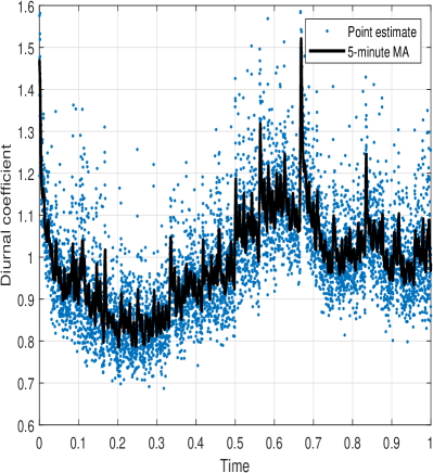
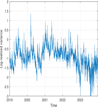
Note. In Panel A, we plot a nonparametric estimator of the intraday periodicity in the spot variance of BTCUSDT. We sample the price process every 15th second from January 1, 2019 to December 31, 2023. Time 0 is midnight in Coordinated Universal Time (UTC). The line is a 5-minute moving average. In Panel B, we plot the daily realized variance (expressed in annualized standard deviation terms) computed after removal of the estimated diurnal pattern. The latter has been log-transformed.

In the Panel A of Figure 1, we plot an estimate of the intraday periodicity in the spot variance of the cryptocurrency market. Here, BTCSUDT serves as a illustration, but in general the volatility of the various exchange rates exhibit near-identical behavior, indicative of a strong commonality. We employ the nonparametric estimator of Taylor and Xu (1997), which averages the time-of-the-day squared 15-second log-returns (a proxy for the average point-in-time intraday variance) and normalizes the sum of these numbers to one to form a seasonality estimate. As readily seen, there is a discernible nonstationary component in the intraday evolution of the volatility of BTCUSDT, which features a complex intraday seasonality pattern. This clashes with our assumed stationarity in (2.1), which can distort the estimation of the stationary Gaussian processes. To avoid this, we pre-filter the 15-second log-return series with the estimated diurnal coefficient to ensure that the rescaled time series is closer to stationary.

We next construct a non-overlapping 2-hour realized variance, which is input into the numerical optimization procedure. To ensure that price jumps do not interfere with our estimation results, we zero out too large absolute log-returns with the truncation approach of Mancini (2009). In Panel B of Figure 1, we plot the resulting log-daily realized variance series, adding up the local diurnal-corrected realized variance estimates to the daily horizon. As expected, it displays a lot of persistence. The typical value of realized variance across currencies is shown in Table 5. The estimates imply that the diffusive variance is rather high, on average, and somewhat in line with the overall level of the total quadratic return variation often seen in individual stocks.

The two stationary Gaussian processes from Section 3 are estimated following the design from Section 4. To get a gauge at the magnitude of the standard errors inherent in the parameter estimates, we employ a parametric bootstrap with 1,000 repetitions. The results are presented in the right-hand side of Table 5. We only include the parameters relating to the acf, since the mean is always estimated in line with the sample average of log-realized variance.

We observe that the roughness index of log-spot variance is located around -0.40 for the fOU process, which we recall is related to the Hurst exponent via the relation $\alpha=H-1/2$. Hence, as consistent with the recent literature on rough volatility, we uncover that there is overwhelming evidence in support of the variance process being more erratic than a standard Brownian motion at short time scales (see, e.g. Bolko, Christensen, Pakkanen, and Veliyev, 2023; Fukasawa, Takabatake, and Westphal, 2022; Gatheral, Jaisson, and Rosenbaum, 2018; Wang, Xiao, and Yu, 2023). The $\kappa$ parameter is very close to zero, so the process exhibits near-unit root behavior.

Turning next to the Cauchy class, the results are striking. On the one hand, $\alpha$ is now estimated around -0.20. While the values are much higher than for the fOU process, they are still located far in roughness space. On the other hand, $\beta$ is estimated far in the long memory range around 0.30 – 0.35. Noting that the link between $\beta$ and the fractional differencing parameter $d$ in a discrete-time ARFIMA($p$,$d$,$q$) process is $\beta=1-2d$ (see Brockwell and Davis, 1991, equation 13.2.1), this corresponds to a $d$ of about 0.30 – 0.40, on average. This agrees with early evidence from the literature on modeling and forecasting realized variance as a fractionally integrated process, see, e.g., Andersen, Bollerslev, Diebold, and Labys (2000), who report that $d\simeq 0.40$ for foreign exchange rates.

Figure 2: Heatmap of composite likelihood function for BTCUSDT.

Panel A: fOU.	Panel B: Cauchy.

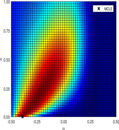
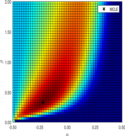
Note. We create a heatmap of the composite likelihoood function for the fOU process (in Panel A) and Cauchy class (in Panel B). A cooler/warmer temperature (blue/red) indicates that the likelihood is lower/higher. We fix the mean and standard deviation ($\mu$ and $\nu$) at the sample average and sample standard deviation of the log-realized variance and vary the remaining free parameters over a broad range of the parameter space. The MCLE is reported with a black cross.

In Figure 2, we construct a heatmap of the composite likelihood function for the BTCUSDT spot exchange rate. Panel A is for the fOU process, while Panel B is for the Cauchy class. To reduce the plot to a two-dimensional plane, we fix $\mu$ and $\nu$ at the sample average and sample standard deviation of the log-realized variance, while varying $\kappa$ and $\beta$ over a broad range of the parameter space and $\alpha$ through the permissible area. The color code indicates the height of the likelihood function with higher (lower) contour values being indicated as a warmer (cooler) temperature.

As consistent with the parameter estimates of BTCUSDT from Table 5, Panel A of Figure 2 indicates that the CL of the fOU process prefers a rough dynamic with a Hurst exponent less than a half. The optimal value of the mean reversion hovers close to the boundary of the parameter space at zero, where the fOU process becomes a scaled version of the non-stationary fBm. Shi and Yu (2022) look at the discrete-time ARFIMA($1$,$d$,$0$) model: $(1-\phi L)(Y_{t}-\mu)=\sigma_{\epsilon}(1-L)^{-d}\epsilon_{t}$, where $L$ is the lag operator and $\epsilon_{t}\sim D(0,1)$ is a white noise. They note that $\phi=0$ and $d=0.5$ is observationally equivalent to $\phi=1$ and $d=-0.5$, leading to identification failure, see also Liu, Shi, and Yu (2020) and Li, Phillips, Shi, and Yu (2023). This can be interpreted as either fast mean reversion and long memory or no mean reversion and anti-persistence. This agrees with a first impression of the likelihood function: the fOU model is prepared to trade roughness for additional mean reversion with only a minimal drop in likelihood and the surface appears to exhibit a plateau over an extended region in that direction. This is a symptom that the model is scrambling to fit both ends of the acf.

However, to get a better gauge at the exact curvature, in Figure 3 we include the profile composite likelihood function of the fOU process in Panel A, $CL_{\alpha}(\kappa)=\max_{\alpha}CL(\alpha,\kappa)$ and the Cauchy class in Panel B, $CL_{\alpha}(\beta)=\max_{\alpha}CL(\alpha,\beta)$. We again set $\mu$ and $\nu$ equal to the sample average and sample standard deviation of the log-realized variance and suppress their influence on the composite likelihood. We then plot this as a function of $\kappa$ or $\beta$ after maximizing with respect to $\alpha$, where the optimal value of the latter is shown on the right-hand $y$-axis. To make the graphs comparable, we normalize the profile likelihood to reach a maximum of one. Overall, the evolution of the fOU profile likelihood in Panel A shows that it is, in fact, monotonically increasing toward the boundary of the parameter space, whereas the Cauchy class has a maximum in the interior. It is interesting to observe that as $\kappa$ increases for the fOU, the optimal value of $\alpha$ does not venture into the long memory region but levels out around zero.

Figure 3: Profile composite likelihood function for BTCUSDT.

Panel A: fOU.	Panel B: Cauchy.

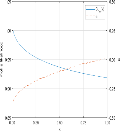
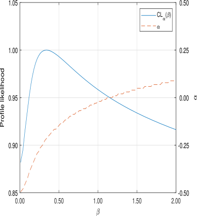
Note. We show the profile composite likelihood function of the fOU process in Panel A, $CL_{\alpha}(\kappa)=\max_{\alpha}CL(\alpha,\kappa)$ and the Cauchy class in Panel B, $CL_{\alpha}(\beta)=\max_{\alpha}CL(\alpha,\beta)$. We fix $\mu$ and $\nu$ at the sample average and sample standard deviation of the log-realized variance. We then plot the composite likelihood as a function of $\kappa$ or $\beta$ after maximizing with respect to $\alpha$, where the optimal value of the latter is shown on the right-hand $y$-axis.

At the end of the day, the fOU process has to make a decision: roughness or long memory. It selects roughness to capture the initial decline in the acf and to fit the subsequent slow decay it forces the mean reversion parameter near zero to approximate long-range dependence. However, the Cauchy class does not suffer from this shortcoming and is able to separate these effects to demonstrate that both are required to describe the data. The $(\alpha,\beta)$ estimate is within the interior of the parameter space and appears to be identified with a high degree of accuracy, gauging from the heatmap, profile likelihood, and the magnitude of the standard errors.

In sum, our empirical results from the Cauchy class of stationary Gaussian processes translate to a non-integrable acf with a sharp initial decline, i.e. roughness, followed by a slow decay toward zero, i.e. long memory. Our results thus provide compelling evidence that spot variance exhibits both roughness and long memory.

6 Conclusion

In this paper, we develop a framework for doing composite likelihood inference of a parametric class of stationary Gaussian processes. We derive the consistency and asymptotic distribution of the maximum composite likelihood estimator (MCLE) under various degrees of persistence.

As an adaptation, we back out the parameters of a fractional Ornstein-Uhlenbeck (fOU) process. In comparison to the method-of-moments estimator (MME) from Wang, Xiao, and Yu (2023), the composite likelihood estimator has the advantage that the full parameter vector is estimated in a single loop rather than via a two-step approach. Moreover, in a simulation study we demonstrate superior finite sample properties of the MCLE over the MME. This is possibly because the MME requires in-fill asymptotic theory, which may not kick in fast enough with realistic choices of sampling frequency.

In our empirical implementation of the fOU process, we discover that the log-variance of the large-cap segment of the cryptocurrency spot exchange rate market exhibits roughness. On the one hand, this agrees with Gatheral, Jaisson, and Rosenbaum (2018) and the universality of the volatility formation process, see Rosenbaum and Zhang (2022). On the other hand, it stands in contrast to the long memory version of the fOU process, proposed as a model for stochastic volatility in Comte and Renault (1998), and the abundant literature on modeling and forecasting realized variance as a long-range dependent variable, e.g. Andersen, Bollerslev, Diebold, and Labys (2003) and Corsi (2009). This “volatility puzzle” is scrutinized further in Shi and Yu (2022), who note that the likelihood function of a discrete-time version of the fOU is bimodal, leading to near-observational equivalence between these two opposing regimes. Li, Phillips, Shi, and Yu (2023) explore the issue in terms of weak identification and the empirical evidence of their identification robust inference is rooting for long memory.

In our opinion, the source of the dispute is that the fOU specification is not flexible enough. It has to control both the short- and long-term persistence in a single parameter—the Hurst exponent. As it cannot accommodate both, it therefore needs to make a stance: roughness or long memory.

Set against this backdrop, a logical step is to divert more attention toward models that decouple the short- and long-run persistence. There are numerous ways one can do that. A standard approach in the SV literature is to superposition independent driving factors (see, e.g., Alizadeh, Brandt, and Diebold, 2002; Barndorff-Nielsen and Shephard, 2002; Christoffersen, Jacobs, and Mimouni, 2010). However, such multi-factor models usually exhibit exponentially decaying acf and, hence, at best approximate roughness and long memory. An intriguing avenue for further research is to superposition two independent fOU processes and check whether the empirical estimates of the Hurst indexes are located on either side of the memory spectrum.

Gneiting and Schlather (2004) proposed a so-called Cauchy class of Gaussian processes. As the fOU, it has three parameters to fit the acf, but—opposite the fOU—it reserves one to fit the short-run persistence and another one to fit the long-run persistence. Bennedsen, Lunde, and Pakkanen (2022) implement this model with MME on a vast cross-sectional set of empirical high-frequency equity data and find that both roughness and long memory are embedded in the log-variance process. In the present paper, we also adopt this strategy to explore the issue based on transaction price data from the cryptocurrency market. Interestingly, our empirical MCLE of the Cauchy class also point toward roughness and long memory being present in the log-spot variance. Thus, our results can help to reconcile the conflicting evidence in the previous literature.

At the moment, our procedure suffers from the fact that spot volatility is latent. The sampling variation inherent in estimators, such as realized variance, impairs the MCLE and causes a potentially severe degree of spurious roughness. Bolko, Christensen, Pakkanen, and Veliyev (2023) account for this in their GMM estimation of the fOU model. In future research, we should attempt to do this as well.

Appendix A Mathematical proofs

Proof of Theorem 2.1.

We observe that a stationary Gaussian process for which $\lim_{h\rightarrow\infty}\rho_{h}=0$ is strongly mixing and, hence, ergodic (see, e.g., Maruyama, 1949, Theorem 9(ii)). Combined with the stationarity assumption, the ergodic theorem implies that the sample average log-composite likelihood converges in probability to its population counterpart:

$$C_{n}(\theta)\equiv\frac{1}{n}cl(\theta;Y)=\frac{1}{n}\sum_{k_{j}\in Q}\sum_{i=1}^{n-k_{q^{j}}^{j}}\log f_{k^{j}}\big{(}Y_{i}^{k^{j}};\theta\big{)}\overset{\mathbb{P}}{\longrightarrow}\mathbb{E}\Bigg{(}\sum_{k^{j}\in Q}\log f_{k^{j}}\big{(}Y_{1}^{k^{j}};\theta\big{)}\Bigg{)}\equiv C(\theta),$$

as $n\rightarrow\infty$.

If we let $\theta_{0}$ denote the true data-generating value of $\theta$, the information inequality implies that $C(\theta)$ is uniquely maximized at $\theta_{0}$ (e.g., Newey and McFadden, 1994, Lemma 2.2). This requires $\theta_{0}$ is identified from the density function, which holds by Assumption 2.2. Theorem 4.1 and 4.3 in Wooldridge (1994) then establishes the uniform weak law of large numbers for the sequence of $q$-wise likelihood functions. From this, the consistency of $\hat{\theta}_{\text{MCLE}}$ follows. $\blacksquare$

Proof of Theorem 2.2.

We recall that

$$cl(\theta;y)=\sum_{k^{j}\in Q}\sum_{i=1}^{n-k_{q^{j}}^{j}}\log f_{k^{j}}(y_{i}^{k^{j}};\theta),$$

where

$$f_{k^{j}}(y_{i}^{k^{j}};\theta)=\frac{1}{\sqrt{(2\pi)^{q^{j}}\det\big{(}\Sigma_{k^{j}}(\theta)\big{)}}}\exp\left(-\frac{1}{2}(y_{i}^{k^{j}})^{\top}\Sigma_{k^{j}}^{-1}(\theta)y_{i}^{k^{j}}\right),$$

and $\Sigma_{k^{j}}=\text{cov}(Y_{i}^{k^{j}})$, which is independent of $i$ by stationarity. Here, we emphasize that the dependence on $\theta$ is solely through $\Sigma$.

The idea is now to compute the score of $cl(\theta;y)$ and expand it around $\theta_{0}$. We next derive an expression for the variance of the score to determine the rate of convergence. The limiting distribution is then found with the help of Breuer and Major (1983), Arcones (1994), Hosking (1996), and Beran, Feng, Ghosh, and Kulik (2013) for the various settings covered in the theorem.

To calculate the score, we write

$$cl(\theta;y)=\sum_{k^{j}\in Q}\sum_{i=1}^{n-k_{q^{j}}^{j}}\left(C-\frac{1}{2}\log\det\big{(}\Sigma_{k^{j}}(\theta)\big{)}-\frac{1}{2}(y_{i}^{k^{j}})^{\top}\Sigma_{k^{j}}^{-1}(\theta)y_{i}^{k^{j}}\right),$$

where $C$ is a constant.

Now, define

$$\begin{split}s_{n}(\theta)&=\frac{\partial}{\partial\theta}cl(\theta;y)\\ &=\left[\sum_{k^{j}\in Q}\sum_{i=1}^{n-k_{q^{j}}^{j}}\left(-\frac{1}{2}\frac{\partial}{\partial\theta_{r}}\log\det\big{(}\Sigma_{k^{j}}(\theta)\big{)}-\frac{1}{2}(y_{i}^{k^{j}})^{\top}\frac{\partial}{\partial\theta_{r}}\Sigma_{k^{j}}^{-1}(\theta)y_{i}^{k^{j}}\right)\right]_{r=1}^{p}\end{split}$$ (A.1)

By definition $s_{n}(\hat{\theta}_{\text{MCLE}})=0$, so from the mean value theorem there exists an interior point, $\bar{\theta}$, on the line segment in $\mathbb{R}^{p}$ connecting $\theta_{0}$ and $\hat{\theta}_{\text{MCLE}}$, such that

$$0=s_{n}(\hat{\theta}_{\text{MCLE}})=s_{n}(\theta_{0})+\frac{\partial}{\partial\theta^{\top}}s_{n}(\bar{\theta})(\hat{\theta}_{\text{MCLE}}-\theta_{0}).$$

After rearranging this expression and multiplying by $\sqrt{n}$, we get:

$$\sqrt{n}(\hat{\theta}_{\text{MCLE}}-\theta_{0})=-\left(\frac{1}{n}\frac{\partial}{\partial\theta^{\top}}s_{n}(\bar{\theta})\right)^{-1}\frac{1}{\sqrt{n}}s_{n}(\theta_{0}).$$

Since $\hat{\theta}_{\text{MCLE}}$ is consistent by Theorem 2.1, we know from the squeeze theorem for convergence in probability that $\bar{\theta}\overset{\mathbb{P}}{\longrightarrow}\theta_{0}$, as $n\rightarrow\infty$, so by stationarity and ergodicity

$$-\frac{1}{n}\frac{\partial}{\partial\theta^{\top}}s_{n}(\bar{\theta})\overset{\mathbb{P}}{\longrightarrow}H(\theta_{0}),$$

as $n\rightarrow\infty$, where

$$H(\theta_{0})=-\mathbb{E}\left(\sum_{k^{j}\in Q}\frac{\partial^{2}}{\partial\theta^{\top}\partial\theta}\log f_{k^{j}}(Y_{1}^{k^{j}};\theta)\mid_{\theta=\theta_{0}}\right)$$

is the negative value of the expected Hessian matrix of $cl(\theta;y)$.

Hence, the main challenge is to derive an expression for the covariance structure of

$$\frac{1}{\sqrt{n}}s_{n}(\theta)=\frac{1}{\sqrt{n}}\left[\sum_{k^{j}\in Q}\sum_{i=1}^{n-k_{q^{j}}^{j}}\left(-\frac{1}{2}\frac{\partial}{\partial\theta_{r}}\log\det\big{(}\Sigma_{k^{j}}(\theta)\big{)}-\frac{1}{2}\frac{\partial}{\partial\theta_{r}}(Y_{i}^{k^{j}})^{\top}\Sigma_{k^{j}}^{-1}(\theta)Y_{i}^{k^{j}}\right)\right]_{r=1}^{p}.$$

Now,

$$(y_{i}^{k^{j}})^{\top}\frac{\partial}{\partial\theta_{r}}\Sigma_{k^{j}}^{-1}(\theta)y_{i}^{k^{j}}=\sum_{j_{1},j_{2}\in k^{j}}y_{i+j_{1}}y_{i+j_{2}}\frac{\partial}{\partial\theta_{r}}(\Sigma_{k^{j}}^{-1}(\theta))_{j_{1},j_{2}},$$

where $\big{(}\Sigma_{k^{j}}^{-1}(\theta)\big{)}_{j_{1},j_{2}}$ is shorthand notation for the entry in $\Sigma_{k^{j}}^{-1}(\theta)$ corresponding to the covariance between $Y_{j_{1}}$ and $Y_{j_{2}}$.

This means we can write

$$\frac{1}{\sqrt{n}}s_{n}(\theta)=\frac{1}{\sqrt{n}}\sum_{k^{j}\in Q}\sum_{i=1}^{n-k_{q^{j}}^{j}}\Bigg{(} -\frac{1}{2}\left[\frac{\partial}{\partial\theta_{r}}\log\det\big{(}\Sigma_{k^{j}}(\theta)\big{)}\right]_{r=1}^{p}$$

$$-\frac{1}{2}\sum_{j_{1},j_{2}\in k^{j}}Y_{i+j_{1}}Y_{i+j_{2}}\left[\frac{\partial}{\partial\theta_{r}}\big{(}\Sigma_{k^{j}}^{-1}(\theta)\big{)}_{j_{1},j_{2}}\right]_{r=1}^{p}\Bigg{)},$$

so we need to calculate

$$\text{var}\left(\frac{1}{\sqrt{n}}\sum_{k^{j}\in Q}\sum_{i=1}^{n-k_{q^{j}}}\sum_{j_{1},j_{2}\in k^{j}}Y_{i+j_{1}}Y_{i+j_{2}}\right),$$

as the rest are additive or multiplicative constants.

Expanding the variance operator, and ignoring the $\sqrt{n}$ for the time being, yields the following calculation:

$$\begin{split}\text{var}&\left(\sum_{k^{j}\in Q}\sum_{i=1}^{n-k_{q^{j}}}\sum_{j_{1},j_{2}\in k^{j}}Y_{i+j_{1}}Y_{i+j_{2}}\right)\\ &=\sum_{k^{j_{1}},k^{j_{2}}\in Q}\sum_{i_{1}=1}^{n-k^{j_{1}}_{q^{j_{1}}}}\sum_{i_{2}=1}^{n-k^{j_{2}}_{q^{j_{2}}}}\sum_{\iota_{1},\iota_{2}\in k^{j_{1}}}\sum_{\iota_{3},\iota_{4}\in k^{j_{2}}}\mathbb{E}[Y_{i_{1}+\iota_{1}}Y_{i_{1}+\iota_{2}}Y_{i_{2}+\iota_{3}}Y_{i_{2}+\iota_{4}}]-\mathbb{E}[Y_{i_{1}+\iota_{1}}Y_{i_{1}+\iota_{2}}]\mathbb{E}[Y_{i_{2}+\iota_{3}}Y_{i_{2}+\iota_{4}}]\\ &=\sum_{k^{j_{1}},k^{j_{2}}\in Q}\sum_{i_{1}=1}^{n-k^{j_{1}}_{q^{j_{1}}}}\sum_{i_{2}=1}^{n-k^{j_{2}}_{q^{j_{2}}}}\sum_{\iota_{1},\iota_{2}\in k^{j_{1}}}\sum_{\iota_{3},\iota_{4}\in k^{j_{2}}}\big{(}\mathbb{E}[Y_{i_{1}+\iota_{1}}Y_{i_{1}+\iota_{2}}]\mathbb{E}[Y_{i_{2}+\iota_{3}}Y_{i_{2}+\iota_{4}}]\\ &+\mathbb{E}[Y_{i_{1}+\iota_{1}}Y_{i_{2}+\iota_{3}}]\mathbb{E}[Y_{i_{1}+\iota_{2}}Y_{i_{2}+\iota_{4}}]+\mathbb{E}[Y_{i_{1}+\iota_{1}}Y_{i_{2}+\iota_{4}}]\mathbb{E}[Y_{i_{1}+\iota_{2}}Y_{i_{2}+\iota_{3}}]\big{)}-\mathbb{E}[Y_{i_{1}+\iota_{1}}Y_{i_{1}+\iota_{2}}]\mathbb{E}[Y_{i_{2}+\iota_{3}}Y_{i_{2}+\iota_{4}}]\\ &=\sum_{k^{j_{1}},k^{j_{2}}\in Q}\sum_{i_{1}=1}^{n-k^{j_{1}}_{q^{j_{1}}}}\sum_{i_{2}=1}^{n-k^{j_{2}}_{q^{j_{2}}}}\sum_{\iota_{1},\iota_{2}\in k^{j_{1}}}\sum_{\iota_{3},\iota_{4}\in k^{j_{2}}}\gamma_{i_{1}+\iota_{1}-(i_{2}+\iota_{3})}\gamma_{i_{1}+\iota_{2}-(i_{2}+\iota_{4})}+\gamma_{i_{1}+\iota_{1}-(i_{2}+\iota_{4})}\gamma_{i_{1}+\iota_{2}-(i_{2}+\iota_{3})}\\ &\sim\sum_{k^{j_{1}},k^{j_{2}}\in Q}\sum_{l=-n}^{n}\sum_{\iota_{1},\iota_{2}\in k^{j_{1}}}\sum_{\iota_{3},\iota_{4}\in k^{j_{2}}}(n-l)\left(\gamma_{l+\iota_{1}-\iota_{3}}\gamma_{l+\iota_{2}-\iota_{4}}+\gamma_{l+\iota_{1}-\iota_{4}}\gamma_{l+\iota_{2}-\iota_{3}}\right).\end{split}$$ (A.2)

where $\gamma_{\ell}$ is the autocovariance of $Y$ at lag $\ell$, and Isserlis’ theorem helps to express higher-order moments of the multivariate normal distribution in terms of its covariance matrix. Thus, convergence of the variance amounts to studying the limiting behavior of the sum of products of autocovariances in (A.2).

In the first part of Theorem 2.2, i.e. the short memory setting and long memory setting with $\beta>1/2$, the sum converges. Here, we can derive the asymptotic distribution using a Breuer-Major theorem, which was introduced in the one-dimensional case in Breuer and Major (1983) and extended to the multivariate setting in Arcones (1994). From (A.1), we see that the score is a quadratic form of $Y$ and, hence, consists of functionals that are either sums of squares or sums of products that are $k^{j}$ periods apart. Since $\rho(h)=O(h^{-\beta})$ for some $\beta>1/2$, the autocovariance function is square-integrable, so we are done if we can prove that the functions from $\mathbb{R}^{2}\rightarrow\mathbb{R}$ given by

$$f:(x,y)\mapsto x^{2}+y^{2}\qquad\text{and}\qquad g:(x,y)\mapsto xy$$

are of Hermite rank 2.

We recall that a function $h$ is of Hermite rank $q$ with respect to a Gaussian process $X$ if (a) $\mathbb{E}\big{(}[h(X)-\mathbb{E}(h(X))]p_{m}(X)\big{)}=0$ for every polynomial $p_{m}$ of degree $m\leq q-1$ and (b) there exists a polynomial $p_{q}$ of degree $q$ such that $\mathbb{E}\big{(}[h(X)-\mathbb{E}(h(X))]p_{q}(X)\big{)}\neq 0$. One can always transform the problem to the multivariate standard normal distribution, because the Hermite rank is invariant under linear mappings. To prove (a), note that

$$\mathbb{E}\bigg{[}h(Z)\prod_{i=0}^{1}H_{\alpha_{i}}(Z_{i})\bigg{]}=0,$$ (A.3)

where $h\in\{f,g\}$, $\alpha=(\alpha_{0},\alpha_{1})\in\{(1,0),(0,1)\}$, $H_{i}$ is the $i$th Hermite polynomial, and $Z=(Z_{1},Z_{2})^{\top}\sim N(0,I_{2})$. (A.3) follows from independence and the zero skewness of the normal distribution, since $H_{0}(x)=1$ and $H_{1}(x)=x$. The claim in (b) follows, because the expectation is nonzero with a second-degree Hermite polynomial, $H_{2}(x)=x^{2}-1$. So the score converges to a Gaussian distribution, and by Slutsky’s theorem so does $\hat{\theta}_{\text{MCLE}}$:

$$\frac{1}{\sqrt{n}}s_{n}(\theta_{0})\overset{d}{\longrightarrow}N(0,V_{0}),$$

where

$$V_{0} =\frac{1}{4}\sum_{k^{j_{1}},k^{j_{2}}\in Q}\sum_{l=-\infty}^{\infty}\sum_{\iota_{1},\iota_{2}\in k^{j_{1}}}\sum_{\iota_{3},\iota_{4}\in k^{j_{2}}}\left[\frac{\partial}{\partial\theta_{r}}\big{(}\Sigma_{k^{j_{1}}}^{-1}(\theta)\big{)}_{\iota_{1},\iota_{2}}|_{\theta=\theta_{0}}\right]_{r=1}^{p}\left(\left[\frac{\partial}{\partial\theta_{r}}\big{(}\Sigma_{k^{j_{2}}}^{-1}(\theta)\big{)}_{\iota_{3},\iota_{4}}|_{\theta=\theta_{0}}\right]_{r=1}^{p}\right)^{\top}$$

$$\times\left(\gamma_{l+\iota_{1}-\iota_{3}}\gamma_{l+\iota_{2}-\iota_{4}}+\gamma_{l+\iota_{1}-\iota_{4}}\gamma_{l+\iota_{2}-\iota_{3}}\right),$$

see Lemma A.1 below.

Next, take $\beta=1/2$. Here, we know from the derivations in (A.2) that the variance of the score, for $n$ large, essentially behaves as

var $$\left(\sum_{k^{j}\in Q}\sum_{i=1}^{n-k_{q^{j}}}\sum_{j_{1},j_{2}\in k^{j}}Y_{i+j_{1}}Y_{i+j_{2}}\right)$$

$$\sim\sum_{k^{j_{1}},k^{j_{2}}\in Q}\sum_{l=-n}^{n}\sum_{\iota_{1},\iota_{2}\in k^{j_{1}}}\sum_{\iota_{3},\iota_{4}\in k^{j_{2}}}(n-l)\left(\gamma_{l+\iota_{1}-\iota_{3}}\gamma_{l+\iota_{2}-\iota_{4}}+\gamma_{l+\iota_{1}-\iota_{4}}\gamma_{l+\iota_{2}-\iota_{3}}\right)$$

$$\sim n\text{var}(Y)+\sum_{k^{j_{1}},k^{j_{2}}\in Q}\sum_{l=-n}^{n}\sum_{\iota_{1},\iota_{2}\in k^{j_{1}}}\sum_{\iota_{3},\iota_{4}\in k^{j_{2}}}\mathbf{1}_{\mathcal{S}}(l,\iota_{1},\iota_{2},\iota_{3},\iota_{4})(n-l)$$

$$\times\left(\frac{L_{\infty}(l+\iota_{1}-\iota_{3})}{\sqrt{|l+\iota_{1}-\iota_{3}|}}\frac{L_{\infty}(l+\iota_{2}-\iota_{4})}{\sqrt{|l+\iota_{2}-\iota_{4}|}}+\frac{L_{\infty}(l+\iota_{1}-\iota_{4})}{\sqrt{|l+\iota_{1}-\iota_{4}|}}\frac{L_{\infty}(l+\iota_{2}-\iota 3)}{\sqrt{|l+\iota_{2}-\iota_{3}|}}\right)$$

$$\sim n\text{var}(Y)+\sum_{l=1}^{n}(n-l)L_{\infty}^{2}(l)l^{-1},$$

where $\mathcal{S}=\{l+\iota_{1}-\iota_{3}\neq 0,l+\iota_{2}-\iota_{4}\neq 0,l+\iota_{1}-\iota_{4}\neq 0,l+\iota_{2}-\iota_{3}\neq 0\}$.

We conclude from this and Lemma A.1 that $\text{var}(n^{-1/2}s_{n}(\theta))=O(L_{\gamma}(n))$, where $L_{\gamma}(n)=\sum_{l=1}^{n}L_{\infty}^{2}(l)l^{-1}$. By formula 1.5.8 and Proposition 1.5.9a in Bingham, Goldie, and Teugels (1989), $L_{\gamma}$ is slowly varying and growing faster than $L_{\infty}^{2}$, so the correct scaling of $s_{n}(\theta)$ is $n^{-1/2}L_{\gamma}^{-1/2}(n)$.

Next, we deduce the limiting distribution of $n^{-1/2}L_{\gamma}^{-1/2}(n)s_{n}(\theta)$. Following Hosking (1996) and Rosenblatt (1979), the $r$th order cross-cumulant of

$$C_{k}=\sqrt{n}L_{\gamma}^{-1/2}(n)\left(\frac{1}{n}\sum_{t=1}^{n-k}Y_{t}Y_{t+k}\right),$$

for $k=0,\dots,l$, is given by

$$u_{r}=\frac{1}{2}\sum(r-1)!(nL_{\gamma}(n))^{-r/2}\sum_{j_{1}=1}^{n}\dots\sum_{j_{r}=1}^{n}\gamma_{j_{1}\pm\alpha_{1}-j_{2}}\gamma_{j_{2}\pm\alpha_{2}-j_{3}}\cdots\gamma_{j_{r-1}\pm\alpha_{r-1}-j_{r}}\gamma_{j_{r}\pm\alpha_{r}-j_{1}},$$

where $\alpha_{i}\in\{0,1,\dots,l\}$, and the outer sum goes over all possible $2^{r}$ combinations of $+$ and $-$ signs in the equation above.

We shall show that for $r\geq 3$, $C_{r}\rightarrow 0$ as $n\rightarrow\infty$. As in Hosking (1996), we set $\alpha_{i}=0$ for convenience. Then, by Cauchy-Schwarz’s inequality

$$|u_{r}|\leq 2^{r-1}(r-1)!(nL_{\gamma}(n))^{-r/2}\sum_{j_{1}=1}^{n}\dots\sum_{j_{r}=1}^{n}\gamma_{j_{1}-j_{2}}^{2}|\gamma_{j_{2}-j_{3}}\cdots|\gamma_{j_{r-1}-j_{r}}|.$$

Now, for $j=1,\dots,n$,

$$\begin{split}\sum_{i=1}^{n}|\gamma_{i-j}|&=\gamma_{0}+\sum_{i=1}^{j-1}|\gamma_{i}|+\sum_{i=1}^{n-j}|\gamma_{i}|\\ &\leq C\big{(}1+L_{\infty}(j)j^{1/2}+L_{\infty}(n-j)(n-j)^{1/2}\big{)}\\ &=O(L_{\infty}(n)n^{1/2}),\end{split}$$

where Karamata’s integral inequality is used in the first passage. Moreover,

$$\sum_{i=1}^{n}\gamma_{i-j}^{2} =\gamma_{0}^{2}+\sum_{i=1}^{j-1}\gamma_{i}^{2}+\sum_{i=1}^{n-j}\gamma_{i}^{2}$$

$$\leq C\big{(}1+L_{\gamma}(j)+L_{\gamma}(n-j)\big{)}$$

$$=O(L_{\gamma}(n)).$$

Holding these results together,

$$u_{r} =(nL_{\gamma}(n))^{-r/2}O(L_{\gamma}(n))O(n^{r/2-1}[L_{\infty}^{2}(n)]^{r/2-1})n$$

$$=O\big{(}L^{1-r/2}_{\gamma}(n)[L_{\infty}^{2}(n)]^{r/2-1}\big{)},$$

following the remark above where $L_{\gamma}$ was introduced. So for $r\geq 3$, $u_{r}\rightarrow 0$ as $n\rightarrow\infty$. This implies a Gaussian limit, as claimed.

At last, we handle the very long memory setting with $\beta\in(0,1/2)$. First, we write

$$n^{\beta}L_{2}^{-1/2}(n)(\hat{\theta}_{\text{MCLE}}-\theta_{0})=-\left(\frac{1}{n}\frac{\partial}{\partial\theta^{\top}}s_{n}(\bar{\theta})\right)^{-1}n^{\beta-1}L_{2}^{-1/2}(n)s_{n}(\theta_{0}).$$

By a weak law of large numbers, as $n\rightarrow\infty$,

$$-\frac{1}{n}\frac{\partial}{\partial\theta^{\top}}s_{n}(\bar{\theta})\overset{\mathbb{P}}{\longrightarrow}H(\theta_{0}).$$

Looking at the last factor in the above expression, we note that the rate normalization is exactly as required for sample covariances of totally dependent Hermite-Rosenblatt processes to converge in law, see, e.g., Section 4.4.1.3 of Beran, Feng, Ghosh, and Kulik (2013) (in their notation, $\beta=1-2d$):

$$n^{\beta-1}L_{2}^{-1/2}(n)s_{n}(\theta_{0})\overset{d}{\longrightarrow}\frac{1}{2}\sum_{k^{j}\in Q}\sum_{j_{1},j_{2}\in k^{j}}\left[\frac{\partial}{\partial\theta_{r}}\big{(}\Sigma_{k}^{-1}(\theta)\big{)}_{j_{1},j_{2}}|_{\theta=\theta_{0}}\right]_{r=1}^{p}Z_{2,H}(1).$$

$\blacksquare$

Lemma A.1.

Let $\{x_{k}\}_{k=1}^{\infty}$ be a sequence of positive numbers. Then, it holds that

$$X_{n}=\sum_{k=1}^{n}x_{k}\text{ converges }\Leftrightarrow\tilde{X}_{n}=\sum_{k=1}^{n}\frac{n-k}{n}x_{k}\text{ converges.}$$

Furthermore, if they converge, the limit is identical.

Proof.

As the terms in the sequence are positive, both $X_{n}$ and $\tilde{X}_{n}$ are increasing. Hence, convergence is equivalent to boundedness by monotone convergence theorem. The implication $\Rightarrow$ follows immediately, since $\tilde{X}_{n}\leq X_{n}$.

To show the $\Leftarrow$ part, assume that $\tilde{X}_{n}$ converges. Then it is bounded by some number $C$. Suppose that $X_{n}$ does not converge, which means that it is unbounded, so there is an $N_{1}$ such that $X_{N_{1}}>2C$. Moreover, for any $N_{2}>2N_{1}$, the first $N_{1}$ terms in $\tilde{X}_{N_{2}}$ are at least half as large as the corresponding ones in $X_{N_{2}}$, since $1-N_{1}/N_{2}>1/2$. This implies that $\tilde{X}_{N_{1}}>\frac{1}{2}X_{N_{1}}>C$, which is a contradiction.

To show the limit is identical, suppose that $X_{n}\rightarrow x_{0}$ as $n\rightarrow\infty$. Then, by definition, for any $\epsilon>0$ there exists $N_{1}\in\mathbb{N}$ such that for $n\geq N_{1}$:

$$x_{0}-X_{n}<\epsilon,$$

Pick some $N_{2}>N_{1}$ such that $\frac{N_{2}-N_{1}}{N_{2}}>1-\epsilon$. Then, we observe that

$$0\leq x_{0}-\tilde{X}_{N_{2}} =x_{0}-\sum_{k=1}^{N_{2}}\frac{N_{2}-k}{N_{2}}x_{k}$$

$$\leq x_{0}-\sum_{k=1}^{N_{1}}\frac{N_{2}-k}{N_{2}}x_{k}$$

$$\leq x_{0}-\frac{N_{2}-N_{1}}{N_{2}}\sum_{k=1}^{N_{1}}x_{k}$$

$$=x_{0}-\frac{N_{2}-N_{1}}{N_{2}}X_{N_{1}}$$

$$\leq x_{0}-\frac{N_{2}-N_{1}}{N_{2}}(x_{0}-\epsilon)$$

$$\leq x_{0}-(1-\epsilon)(x_{0}-\epsilon)=\epsilon(1+x_{0}-\epsilon).$$

As $\epsilon(1+x_{0}-\epsilon)$ can be made arbitrarily small, $\tilde{X}_{n}\rightarrow x_{0}$. $\blacksquare$

Appendix B Method of moments-based estimator

In this appendix, we review the method of moments-based estimator of the parameters of the fOU process and the Cauchy class, which serve as a benchmark for our MCLE approach. Our description is based on Wang, Xiao, and Yu (2023) and Bennedsen, Lunde, and Pakkanen (2022). It is not too detailed, but the reader can find further information and references in their papers.

As in the composite likelihood framework, the estimator of the mean, $\mu$, is the sample average, $\hat{\mu}=n^{-1}\sum_{i=1}^{n}Y_{i\Delta}$.

The roughness index, $\alpha$, is estimated by a change-of-frequency (COF) approach (see, e.g. Lang and Roueff, 2001; Barndorff-Nielsen, Corcuera, and Podolskij, 2013). To write this down succinctly, we need a notion of the $k$th-order difference, for any $k\in\mathbb{N}$, of a time series observed with time gap $\Delta$ and sampled at frequency $\eta$, where $\eta\in\mathbb{N}$. At stage $i\geq\eta k$, this can be defined as

$$(1-L^{\eta})^{k}Y_{i\Delta}\equiv\sum_{j=0}^{k}(-1)^{j}\binom{k}{j}Y_{(i-\eta j)\Delta},$$

where $L$ is the lag operator.

We now introduce the $p$th-order realized power variation:

$$V(Y,p,k,\eta;\Delta)_{t}=\sum_{i=\eta k}^{[t/\Delta]}|(1-L^{\eta})^{k}Y_{i\Delta}|^{p},$$

for $p>0$.

The COF estimator of $\alpha$ is then

$$\hat{\alpha}=\frac{\log_{2}(\text{COF}(Y,p,\Delta)_{t})}{p}-\frac{1}{2},\quad\text{where }\text{COF}(Y,p,\Delta)_{t}=\frac{V(Y,p,2,2;\Delta)_{t}}{V(Y,p,2,1;\Delta)_{t}},\quad\text{for }t>0.$$

$\hat{\alpha}$ is a consistent estimator of $\alpha$ in the infill limit as $\Delta\rightarrow 0$. We follow Wang, Xiao, and Yu (2023) and implement $\hat{\alpha}$ with $p=2$. We remark that this estimator is a special case of the one from Bennedsen, Lunde, and Pakkanen (2022).

In the fOU, the standard deviation, $\nu$, and mean reversion, $\kappa$, are estimated as:

$$\hat{\nu}=\sqrt{\frac{\sum_{i=3}^{n}(Y_{i\Delta}-2Y_{(i-1)\Delta}+Y_{(i-2)\Delta})^{2}}{n\big{(}4-2^{2\hat{H}}\big{)}\Delta^{2\hat{H}}}}\quad\text{and}\quad\hat{\kappa}=\left(\frac{n\sum_{i=1}^{n}Y_{i\Delta}^{2}-\left(\sum_{i=1}^{n}Y_{i\Delta}\right)^{2}}{n^{2}\hat{\nu}^{2}\hat{H}\Gamma(2\hat{H})}\right)^{-1/(2\hat{H})},$$

where $\hat{H}=\hat{\alpha}+1/2$.

In the Cauchy class, $\nu$ is recovered directly as the sample standard deviation, $\hat{\nu}=n^{-1}\sum_{i=1}^{n}(Y_{i\Delta}-\hat{\mu})^{2}$. $\beta$ is estimated by matching the theoretical acf from (3.6) to the empirical one with the first-stage estimator of $\alpha$ plugged in, leaving it as a function of $\beta$.

Appendix C Monte Carlo analysis with $N=1$

Presented without comment.

Table 6: Parameter estimation of the fOU process ($\mu$ known).

Parameter	Value	MCLE				MME
		$T=1{,}095$	$T=1{,}825$	$T=2{,}555$		$T=1{,}095$	$T=1{,}825$	$T=2{,}555$
Panel A:
$\mu$	0.000	0.0000 (0.0000)	0.0000 (0.0000)	0.0000 (0.0000)		0.0000 (0.0000)	0.0000 (0.0000)	0.0000 (0.0000)
$\kappa$	0.005	0.0058 (0.0099)	0.0055 (0.0075)	0.0060 (0.0070)		0.0193 (0.0338)	0.0150 (0.0243)	0.0131 (0.0202)
$\nu$	1.250	1.2526 (0.0392)	1.2975 (1.8482)	1.2174 (0.0244)		1.2497 (0.0323)	1.2495 (0.0249)	1.2494 (0.0210)
$\alpha$	-0.450	-0.4651 (0.0215)	-0.4640 (0.0182)	-0.4564 (0.0111)		-0.4461 (0.0384)	-0.4483 (0.0317)	-0.4488 (0.0281)
Panel B:
$\mu$	0.000	0.0000 (0.0000)	0.0000 (0.0000)	0.0000 (0.0000)		0.0000 (0.0000)	0.0000 (0.0000)	0.0000 (0.0000)
$\kappa$	0.010	0.0116 (0.0082)	0.0113 (0.0062)	0.0111 (0.0050)		0.0190 (0.0246)	0.0158 (0.0179)	0.0145 (0.0149)
$\nu$	0.750	0.7238 (0.0189)	0.7191 (0.0144)	0.7265 (0.0144)		0.7490 (0.0187)	0.7493 (0.0145)	0.7494 (0.0123)
$\alpha$	-0.400	-0.4221 (0.0227)	-0.4203 (0.0159)	-0.4151 (0.0128)		-0.4010 (0.0448)	-0.4008 (0.0355)	-0.4002 (0.0302)
Panel C:
$\mu$	0.000	0.0000 (0.0000)	0.0000 (0.0000)	0.0000 (0.0000)		0.0000 (0.0000)	0.0000 (0.0000)	0.0000 (0.0000)
$\kappa$	0.015	0.0203 (0.0092)	0.0192 (0.0068)	0.0183 (0.0055)		0.0181 (0.0125)	0.0168 (0.0093)	0.0164 (0.0077)
$\nu$	0.500	0.5049 (0.0240)	0.5049 (0.0178)	0.5040 (0.0145)		0.4993 (0.0121)	0.4995 (0.0094)	0.4996 (0.0080)
$\alpha$	-0.200	-0.2312 (0.0350)	-0.2319 (0.0266)	-0.2215 (0.0222)		-0.2016 (0.0436)	-0.2009 (0.0338)	-0.2003 (0.0286)
Panel D:
$\mu$	0.000	0.0000 (0.0000)	0.0000 (0.0000)	0.0000 (0.0000)		0.0000 (0.0000)	0.0000 (0.0000)	0.0000 (0.0000)
$\kappa$	0.035	0.0521 (0.0347)	0.0481 (0.0183)	0.0445 (0.0114)		0.0374 (0.0152)	0.0363 (0.0115)	0.0359 (0.0096)
$\nu$	0.300	0.3028 (0.0166)	0.3009 (0.0091)	0.3006 (0.0067)		0.2995 (0.0086)	0.2996 (0.0066)	0.2996 (0.0056)
$\alpha$	0.000	-0.0116 (0.0611)	-0.0142 (0.0397)	-0.0082 (0.0294)		-0.0023 (0.0411)	-0.0015 (0.0318)	-0.0011 (0.0268)
Panel E:
$\mu$	0.000	0.0000 (0.0000)	0.0000 (0.0000)	0.0000 (0.0000)		0.0000 (0.0000)	0.0000 (0.0000)	0.0000 (0.0000)
$\kappa$	0.070	0.1051 (0.0502)	0.1002 (0.0375)	0.0912 (0.0290)		0.0716 (0.0217)	0.0702 (0.0167)	0.0696 (0.0139)
$\nu$	0.200	0.2142 (0.0265)	0.2099 (0.0181)	0.2077 (0.0268)		0.1987 (0.0095)	0.1987 (0.0073)	0.1986 (0.0061)
$\alpha$	0.200	0.1925 (0.0840)	0.1945 (0.0695)	0.1967 (0.0606)		0.1939 (0.0382)	0.1947 (0.0297)	0.1951 (0.0249)

Note. We simulate the process in the caption of the table 10,000 times on the interval $[0,T]$, where $T$ is interpreted as the number of days. There is $N=1$ observation per unit interval, corresponding to a single observation every day. The true value of the parameter vector appear to the left in Panel A – E. We estimate $\theta$ with the maximum composite likelihod estimation (MCLE) procedure developed in the main text, and benchmark it against a method-of-moments estimator (MME). The table reports the Monte Carlo average value of each parameter estimate across simulations (standard deviation in parenthesis).

Table 7: Parameter estimation of the fOU process ($\mu$ estimated).

Parameter	Value	MCLE				MME
		$T=1{,}095$	$T=1{,}825$	$T=2{,}555$		$T=1{,}095$	$T=1{,}825$	$T=2{,}555$
Panel A:
$\mu$	0.000	0.0002 (0.2953)	-0.0020 (0.1925)	-0.0007 (0.2097)		-0.0005 (0.2574)	-0.0022 (0.1634)	-0.0013 (0.1197)
$\kappa$	0.005	0.0081 (0.0117)	0.0066 (0.0082)	0.0064 (0.0068)		0.0223 (0.0372)	0.0162 (0.0257)	0.0137 (0.0210)
$\nu$	1.250	1.2493 (0.0626)	1.2533 (0.0678)	1.2178 (0.0225)		1.2497 (0.0323)	1.2495 (0.0249)	1.2494 (0.0210)
$\alpha$	-0.450	-0.4604 (0.0189)	-0.4620 (0.0171)	-0.4563 (0.0113)		-0.4461 (0.0384)	-0.4483 (0.0317)	-0.4488 (0.0281)
Panel B:
$\mu$	0.000	0.0007 (0.1406)	-0.0001 (0.1062)	-0.0005 (0.0721)		0.0007 (0.0936)	-0.0006 (0.0619)	-0.0002 (0.0464)
$\kappa$	0.010	0.0129 (0.0088)	0.0119 (0.0063)	0.0114 (0.0049)		0.0200 (0.0256)	0.0162 (0.0183)	0.0147 (0.0151)
$\nu$	0.750	0.7224 (0.0180)	0.7184 (0.0142)	0.7260 (0.0143)		0.7490 (0.0187)	0.7493 (0.0145)	0.7494 (0.0123)
$\alpha$	-0.400	-0.4205 (0.0211)	-0.4196 (0.0154)	-0.4148 (0.0126)		-0.4010 (0.0448)	-0.4008 (0.0355)	-0.4002 (0.0302)
Panel C:
$\mu$	0.000	0.0012 (0.0977)	-0.0004 (0.0695)	-0.0003 (0.0554)		0.0011 (0.0968)	-0.0004 (0.0694)	-0.0001 (0.0551)
$\kappa$	0.015	0.0221 (0.0095)	0.0201 (0.0070)	0.0189 (0.0056)		0.0192 (0.0132)	0.0174 (0.0095)	0.0167 (0.0078)
$\nu$	0.500	0.5024 (0.0213)	0.5037 (0.0171)	0.5034 (0.0143)		0.4993 (0.0121)	0.4995 (0.0094)	0.4996 (0.0080)
$\alpha$	-0.200	-0.2284 (0.0325)	-0.2305 (0.0259)	-0.2207 (0.0219)		-0.2016 (0.0436)	-0.2009 (0.0338)	-0.2003 (0.0286)
Panel D:
$\mu$	0.000	0.0006 (0.0677)	-0.0003 (0.0528)	-0.0002 (0.0445)		0.0005 (0.0671)	-0.0003 (0.0523)	-0.0002 (0.0441)
$\kappa$	0.035	0.0511 (0.0193)	0.0487 (0.0139)	0.0452 (0.0106)		0.0393 (0.0157)	0.0375 (0.0117)	0.0367 (0.0097)
$\nu$	0.300	0.3033 (0.0104)	0.3018 (0.0078)	0.3013 (0.0064)		0.2995 (0.0086)	0.2996 (0.0066)	0.2996 (0.0056)
$\alpha$	0.000	-0.0185 (0.0440)	-0.0172 (0.0339)	-0.0097 (0.0276)		-0.0023 (0.0411)	-0.0015 (0.0318)	-0.0011 (0.0268)
Panel E:
$\mu$	0.000	0.0004 (0.0684)	-0.0004 (0.0591)	-0.0003 (0.0532)		0.0003 (0.0681)	-0.0003 (0.0586)	-0.0002 (0.0528)
$\kappa$	0.070	0.0841 (0.0228)	0.0846 (0.0181)	0.0790 (0.0147)		0.0776 (0.0224)	0.0745 (0.0169)	0.0730 (0.0140)
$\nu$	0.200	0.2083 (0.0090)	0.2063 (0.0072)	0.2053 (0.0062)		0.1987 (0.0095)	0.1987 (0.0073)	0.1986 (0.0061)
$\alpha$	0.200	0.1385 (0.0415)	0.1518 (0.0365)	0.1601 (0.0315)		0.1939 (0.0382)	0.1947 (0.0297)	0.1951 (0.0249)

Note. We simulate the process in the caption of the table 10,000 times on the interval $[0,T]$, where $T$ is interpreted as the number of days. There is $N=1$ observation per unit interval, corresponding to a single observation every day. The true value of the parameter vector appear to the left in Panel A – E. We estimate $\theta$ with the maximum composite likelihod estimation (MCLE) procedure developed in the main text, and benchmark it against a method-of-moments estimator (MME). The table reports the Monte Carlo average value of each parameter estimate across simulations (standard deviation in parenthesis).

Table 8: Parameter estimation of the Cauchy class ($\mu$ known).

Parameter	Value	MCLE				MME
		$T=1{,}095$	$T=1{,}825$	$T=2{,}555$		$T=1{,}095$	$T=1{,}825$	$T=2{,}555$
Panel A:
$\mu$	0.000	0.0000 (0.0000)	0.0000 (0.0000)	0.0000 (0.0000)		0.0000 (0.0000)	0.0000 (0.0000)	0.0000 (0.0000)
$\beta$	0.250	0.2324 (0.3645)	0.1916 (0.3063)	0.2510 (0.2842)		0.3005 (0.1830)	0.2651 (0.1546)	0.2444 (0.1404)
$\nu$	1.250	1.1008 (0.0658)	1.1010 (0.0600)	1.1398 (0.0585)		1.2486 (0.0744)	1.2487 (0.0677)	1.2490 (0.0638)
$\alpha$	-0.450	-0.4647 (0.0549)	-0.4711 (0.0460)	-0.4604 (0.0445)		-0.4703 (0.0277)	-0.4743 (0.0217)	-0.4763 (0.0189)
Panel B:
$\mu$	0.000	0.0000 (0.0000)	0.0000 (0.0000)	0.0000 (0.0000)		0.0000 (0.0000)	0.0000 (0.0000)	0.0000 (0.0000)
$\beta$	0.500	0.4489 (0.4067)	0.4331 (0.3559)	0.5009 (0.2766)		0.3767 (0.2034)	0.3516 (0.1777)	0.3377 (0.1645)
$\nu$	0.750	0.6608 (0.0225)	0.6608 (0.0185)	0.6840 (0.0167)		0.7498 (0.0255)	0.7498 (0.0208)	0.7499 (0.0182)
$\alpha$	-0.400	-0.4221 (0.0700)	-0.4252 (0.0612)	-0.4104 (0.0489)		-0.4630 (0.0319)	-0.4666 (0.0258)	-0.4682 (0.0229)
Panel C:
$\mu$	0.000	0.0000 (0.0000)	0.0000 (0.0000)	0.0000 (0.0000)		0.0000 (0.0000)	0.0000 (0.0000)	0.0000 (0.0000)
$\beta$	0.750	0.8201 (0.2204)	0.8154 (0.1594)	0.8019 (0.1305)		0.6934 (0.1227)	0.6881 (0.0977)	0.6833 (0.0881)
$\nu$	0.500	0.4388 (0.0155)	0.4388 (0.0120)	0.4547 (0.0106)		0.4999 (0.0182)	0.4999 (0.0141)	0.4999 (0.0120)
$\alpha$	-0.200	-0.2302 (0.0698)	-0.2315 (0.0502)	-0.2240 (0.0426)		-0.3694 (0.0453)	-0.3687 (0.0351)	-0.3682 (0.0298)
Panel D:
$\mu$	0.000	0.0000 (0.0000)	0.0000 (0.0000)	0.0000 (0.0000)		0.0000 (0.0000)	0.0000 (0.0000)	0.0000 (0.0000)
$\beta$	1.000	1.1073 (0.1954)	1.0978 (0.1497)	1.0770 (0.1243)		0.8829 (0.1044)	0.8743 (0.0876)	0.8696 (0.0789)
$\nu$	0.300	0.2633 (0.0084)	0.2634 (0.0065)	0.2729 (0.0057)		0.2999 (0.0098)	0.2999 (0.0075)	0.2999 (0.0064)
$\alpha$	0.000	-0.0501 (0.0778)	-0.0533 (0.0600)	-0.0398 (0.0517)		-0.2591 (0.0439)	-0.2583 (0.0339)	-0.2577 (0.0287)
Panel E:
$\mu$	0.000	0.0000 (0.0000)	0.0000 (0.0000)	0.0000 (0.0000)		0.0000 (0.0000)	0.0000 (0.0000)	0.0000 (0.0000)
$\beta$	1.250	1.3878 (0.2226)	1.3783 (0.1696)	1.3506 (0.1410)		1.0545 (0.1144)	1.0484 (0.0922)	1.0455 (0.0804)
$\nu$	0.200	0.1757 (0.0054)	0.1757 (0.0041)	0.1820 (0.0036)		0.1999 (0.0062)	0.1999 (0.0048)	0.2000 (0.0040)
$\alpha$	0.200	0.1323 (0.0977)	0.1295 (0.0754)	0.1485 (0.0648)		-0.1490 (0.0421)	-0.1481 (0.0326)	-0.1475 (0.0275)

Note. We simulate the process in the caption of the table 10,000 times on the interval $[0,T]$, where $T$ is interpreted as the number of days. There is $N=1$ observation per unit interval, corresponding to a single observation every day. The true value of the parameter vector appear to the left in Panel A – E. We estimate $\theta$ with the maximum composite likelihod estimation (MCLE) procedure developed in the main text, and benchmark it against a method-of-moments estimator (MME). The table reports the Monte Carlo average value of each parameter estimate across simulations (standard deviation in parenthesis).

Table 9: Parameter estimation of the Cauchy class ($\mu$ estimated).

Parameter	Value	MCLE				MME
		$T=1{,}095$	$T=1{,}825$	$T=2{,}555$		$T=1{,}095$	$T=1{,}825$	$T=2{,}555$
Panel A:
$\mu$	0.000	0.0060 (0.3614)	0.0064 (0.3466)	0.0064 (0.3375)		0.0061 (0.3613)	0.0064 (0.3460)	0.0064 (0.3372)
$\beta$	0.250	0.6365 (0.4285)	0.5861 (0.2933)	0.6150 (0.1713)		0.4550 (0.1967)	0.4032 (0.1648)	0.3755 (0.1506)
$\nu$	1.250	1.0552 (0.0257)	1.0589 (0.0210)	1.0985 (0.0191)		1.1971 (0.0293)	1.2015 (0.0240)	1.2041 (0.0212)
$\alpha$	-0.450	-0.4091 (0.0637)	-0.4141 (0.0435)	-0.4058 (0.0254)		-0.4703 (0.0277)	-0.4743 (0.0217)	-0.4763 (0.0189)
Panel B:
$\mu$	0.000	0.0017 (0.1399)	0.0020 (0.1272)	0.0020 (0.1194)		0.0017 (0.1398)	0.0020 (0.1267)	0.0020 (0.1191)
$\beta$	0.500	0.7635 (0.3343)	0.7261 (0.2302)	0.7154 (0.1509)		0.4892 (0.2040)	0.4542 (0.1760)	0.4349 (0.1626)
$\nu$	0.750	0.6493 (0.0162)	0.6513 (0.0130)	0.6754 (0.0117)		0.7369 (0.0185)	0.7392 (0.0149)	0.7405 (0.0129)
$\alpha$	-0.400	-0.3718 (0.0570)	-0.3770 (0.0386)	-0.3744 (0.0254)		-0.4630 (0.0319)	-0.4666 (0.0258)	-0.4682 (0.0229)
Panel C:
$\mu$	0.000	0.0008 (0.0772)	0.0011 (0.0654)	0.0011 (0.0584)		0.0009 (0.0771)	0.0011 (0.0650)	0.0011 (0.0582)
$\beta$	0.750	0.9248 (0.1780)	0.8846 (0.1372)	0.8567 (0.1148)		0.7756 (0.1085)	0.7615 (0.0774)	0.7519 (0.0639)
$\nu$	0.500	0.4339 (0.0139)	0.4353 (0.0110)	0.4518 (0.0098)		0.4940 (0.0163)	0.4957 (0.0129)	0.4965 (0.0111)
$\alpha$	-0.200	-0.1999 (0.0530)	-0.2112 (0.0411)	-0.2071 (0.0358)		-0.3694 (0.0453)	-0.3687 (0.0351)	-0.3682 (0.0298)
Panel D:
$\mu$	0.000	0.0001 (0.0317)	0.0002 (0.0256)	0.0002 (0.0222)		0.0001 (0.0316)	0.0002 (0.0254)	0.0002 (0.0221)
$\beta$	1.000	1.1584 (0.1955)	1.1302 (0.1488)	1.1010 (0.1238)		0.9489 (0.0840)	0.9274 (0.0680)	0.9159 (0.0601)
$\nu$	0.300	0.2619 (0.0082)	0.2625 (0.0064)	0.2722 (0.0056)		0.2982 (0.0095)	0.2988 (0.0074)	0.2991 (0.0063)
$\alpha$	0.000	-0.0330 (0.0759)	-0.0424 (0.0588)	-0.0314 (0.0510)		-0.2591 (0.0439)	-0.2583 (0.0339)	-0.2577 (0.0287)
Panel E:
$\mu$	0.000	0.0000 (0.0161)	0.0001 (0.0126)	0.0001 (0.0108)		0.0000 (0.0160)	0.0001 (0.0126)	0.0001 (0.0107)
$\beta$	1.250	1.4251 (0.2259)	1.4011 (0.1709)	1.3668 (0.1419)		1.1073 (0.0965)	1.0872 (0.0779)	1.0772 (0.0683)
$\nu$	0.200	0.1751 (0.0053)	0.1754 (0.0041)	0.1818 (0.0036)		0.1993 (0.0061)	0.1995 (0.0047)	0.1997 (0.0040)
$\alpha$	0.200	0.1457 (0.0973)	0.1377 (0.0751)	0.1545 (0.0646)		-0.1490 (0.0421)	-0.1481 (0.0326)	-0.1475 (0.0275)

Note. We simulate the process in the caption of the table 10,000 times on the interval $[0,T]$, where $T$ is interpreted as the number of days. There is $N=1$ observation per unit interval, corresponding to a single observation every day. The true value of the parameter vector appear to the left in Panel A – E. We estimate $\theta$ with the maximum composite likelihod estimation (MCLE) procedure developed in the main text, and benchmark it against a method-of-moments estimator (MME). The table reports the Monte Carlo average value of each parameter estimate across simulations (standard deviation in parenthesis).

References

- (1)
- Alizadeh, Brandt, and Diebold (2002) Alizadeh, S., M. W. Brandt, and F. X. Diebold, 2002, “Range-based estimation of stochastic volatility models,” Journal of Finance, 57(3), 1047–1092.
- Andersen, Bollerslev, Diebold, and Labys (2000) Andersen, T. G., T. Bollerslev, F. X. Diebold, and P. Labys, 2000, “Great realizations,” Risk, 13(3), 105–108.
- Andersen, Bollerslev, Diebold, and Labys (2003) , 2003, “Modeling and forecasting realized volatility,” Econometrica, 71(2), 579–625.
- Arcones (1994) Arcones, M. A., 1994, “Limit theorems for nonlinear functionals of a stationary Gaussian sequence of vectors,” Annals of Probability, 22(4), 2242–2274.
- Asmussen and Glynn (2007) Asmussen, S., and P. W. Glynn, 2007, Stochastic Simulation: Algorithms and Analysis. Springer, Berlin, 1st edn.
- Barndorff-Nielsen, Corcuera, and Podolskij (2013) Barndorff-Nielsen, O., J. M. Corcuera, and M. Podolskij, 2013, “Limit theorems for functionals of higher order differences of Brownian semi-stationary processes,” in Prokhorov and Contemporary Probability Theory, ed. by A. N. Shiryaev, S. R. S. Varadhan, and E. L. Presman. Springer, Heidelberg, pp. 69–96.
- Barndorff-Nielsen and Schmiegel (2009) Barndorff-Nielsen, O. E., and J. Schmiegel, 2009, “Brownian semistationary processes and volatility/intermittency,” in Radon Series on Computational and Applied Mathematics: Advanced Financial Modelling, ed. by H. Albrecher, W. J. Runggaldier, and W. Schachermayer. De Gruyter, Berlin, pp. 1–25.
- Barndorff-Nielsen and Shephard (2002) Barndorff-Nielsen, O. E., and N. Shephard, 2002, “Econometric analysis of realized volatility and its use in estimating stochastic volatility models,” Journal of the Royal Statistical Society: Series B, 64(2), 253–280.
- Bennedsen (2020) Bennedsen, M., 2020, “Semiparametric inference on the fractal index of Gaussian and conditionally Gaussian time series data,” Econometric Reviews, 39(9), 875–903.
- Bennedsen, Lunde, and Pakkanen (2022) Bennedsen, M., A. Lunde, and M. S. Pakkanen, 2022, “Decoupling the short- and long-term behavior of stochastic volatility,” Journal of Financial Econometrics, 20(5), 961–1006.
- Bennedsen, Lunde, Shephard, and Veraart (2023) Bennedsen, M., A. Lunde, N. Shephard, and A. E. D. Veraart, 2023, “Inference and forecasting for continuous-time integer-valued trawl processes,” Journal of Econometrics, 236(2), 105476.
- Beran, Feng, Ghosh, and Kulik (2013) Beran, J., Y. Feng, S. Ghosh, and R. Kulik, 2013, Long-Memory Processes: Probabilistic Properties and Statistical Methods. Springer, Berlin, 1st edn.
- Besag (1974) Besag, J., 1974, “Spatial interaction and the statistical analysis of lattice systems,” Journal of the Royal Statistical Society: Series B, 36(2), 192–236.
- Bingham, Goldie, and Teugels (1989) Bingham, N. H., C. M. Goldie, and J. L. Teugels, 1989, Regular Variation. Cambridge University Press, Cambridge, 1st edn.
- Bolko, Christensen, Pakkanen, and Veliyev (2023) Bolko, A. E., K. Christensen, M. Pakkanen, and B. Veliyev, 2023, “A GMM approach to estimate the roughness of stochastic volatility,” Journal of Econometrics, 235(2), 745–778.
- Brent, Gustavson, and Yun (1980) Brent, R. P., F. G. Gustavson, and D. Y. Y. Yun, 1980, “Fast solution of Toeplitz systems of equations and computation of Padé approximants,” Journal of Algorithms, 1(3), 259–295.
- Breuer and Major (1983) Breuer, P., and P. Major, 1983, “Central limit theorems for non-linear functionals of Gaussian fields,” Journal of Multivariate Analysis, 13(3), 425–441.
- Brockwell and Davis (1991) Brockwell, P. J., and R. A. Davis, 1991, Time Series: Theory and Methods. Springer, Berlin, 1st edn.
- Chentsov (1956) Chentsov, N. N., 1956, “Weak convergence of stochastic processes whose trajectories have no discontinuities of the second kind and the “heuristic” approach to the Kolmogorov-Smirnov test,” Theory of Probability and Its Applications, 1(1), 140–144.
- Cheridito, Kawaguchi, and Maejima (2003) Cheridito, P., H. Kawaguchi, and M. Maejima, 2003, “Fractional Ornstein-Uhlenbeck processes,” Electronic Journal of Probability, 8(3), 1–14.
- Chong and Todorov (2023) Chong, C. H., and V. Todorov, 2023, “The Fine Structure of Volatility Dynamics,” Working paper, Hong Kong University of Science and Technology (HKUST).
- Christensen, Thyrsgaard, and Veliyev (2019) Christensen, K., M. Thyrsgaard, and B. Veliyev, 2019, “The realized empirical distribution function of stochastic variance with application to goodness-of-fit testing,” Journal of Econometrics, 212(2), 556–583.
- Christoffersen, Jacobs, and Mimouni (2010) Christoffersen, P. F., K. Jacobs, and K. Mimouni, 2010, “Volatility dynamics for the S&P500: Evidence from realized volatility, daily returns, and option prices,” Review of Financial Studies, 23(8), 3141–3189.
- Comte and Renault (1998) Comte, F., and E. Renault, 1998, “Long memory in continuous-time stochastic volatility models,” Mathematical Finance, 8(4), 291–323.
- Corsi (2009) Corsi, F., 2009, “A simple approximate long-memory model of realized volatility,” Journal of Financial Econometrics, 7(2), 174–196.
- Cox and Reid (2004) Cox, D. R., and N. Reid, 2004, “A note on pseudolikelihood constructed from marginal densities,” Biometrika, 91(3), 729–737.
- Davis and Yau (2011) Davis, R. A., and C. Y. Yau, 2011, “Comments on pairwise likelihood in time series models,” Statistica Sinica, 21(1), 255–277.
- Durbin (1960) Durbin, J., 1960, “The fitting of time-series models,” Review of the International Statistical Institute, 28(3), 233–244.
- Fukasawa, Takabatake, and Westphal (2022) Fukasawa, M., T. Takabatake, and R. Westphal, 2022, “Consistent estimation for fractional stochastic volatility model under high-frequency asymptotics,” Mathematical Finance, 32(4), 1086–1132.
- Garnier and Sølna (2018) Garnier, J., and K. Sølna, 2018, “Option pricing under fast-varying and rough stochastic volatility,” Annals of Finance, 14(4), 489–516.
- Gatheral, Jaisson, and Rosenbaum (2018) Gatheral, J., T. Jaisson, and M. Rosenbaum, 2018, “Volatility is rough,” Quantitative Finance, 18(6), 933–949.