Robust Fuel-Optimal Landing Guidance for Hazardous Terrain using Multiple Sliding Surfaces

Abstract

In any spacecraft landing mission, precision soft landing in a fuel-efficient way while also avoiding nearby hazardous terrain is of utmost importance. Very few existing literature have attempted addressing both the problems of precision soft landing and terrain avoidance simultaneously. To this end, an optimal terrain avoidance landing guidance (OTALG) was recently developed, which showed promising performance in avoiding the terrain while consuming near-minimum fuel. However, its performance significantly degrades in the face of external disturbances, indicating lack of robustness. In order to mitigate this problem, in this paper, a novel near fuel-optimal guidance law is developed to avoid terrain and land precisely and softly at the desired landing site, under atmospheric perturbations and thrust deviations and constraints. Expanding the OTALG formulation by using sliding mode control with multiple sliding surfaces (MSS), the presented guidance law, named ‘MSS-OTALG’, improves in terms of precision soft landing accuracy. Further, the sliding parameter is designed to allow the lander to avoid terrain by leaving the trajectory enforced by the sliding mode, and eventually returning to it when the terrain avoidance phase is completed. And finally, the robustness of the MSS-OTALG is established by proving practical fixed-time stability. Extensive numerical simulations are also presented to showcase its performance in terms of terrain avoidance, low fuel consumption and accuracy of precision soft landing. Comparative studies against existing relevant literature validates a balanced trade-off of all these performance measures achieved by the developed MSS-OTALG.

1 INTRODUCTION

The key objective of extra-planetary landing missions is to collect samples, analyse them and relay the data back to Earth. The lander needs to carry an extensive set of scientific module, avoid any damage during the entry, descent and landing (EDL) phase and land as close to the area of interest as possible, even under disturbances and uncertainties, to get the most out of these missions. To facilitate this, studying fuel optimality, terrain avoidance, and robustness is crucial for EDL missions. Modern Mars missions such as Curiosity, Tianwen-1, and Perseverance have successfully been able to reduce the landing error ellipse’s axis length to less than 100km [1, 2].

Fuel optimality and precision soft-landing accuracy have been significantly researched since the first attempt at reaching a celestial body. Methods ranging from feedback guidance, nonlinear control, optimal control, convex optimisation, and learning-based methods have been studied in the literature to reach the desired landing site safely and precisely. To address the nonconvexities associated with the landing guidance problems, algorithms such as Lossless Convexification (LCvx) and Successive Convexification (SCvx) have been developed [3, 4]. However, convexification-based methods are open-loop and, therefore, highly susceptible to perturbations and estimation errors. Classical feedback laws for missile guidance, like Proportional Navigation Guidance (PNG), and its adaptations, such as biased PNG [5], have been explored for powered descent. The concept of zero-effort-miss (ZEM) is extensively used in missile guidance, which denotes the miss distance from the desired terminal position if no control effort is applied from the current time forward. The idea of ZEM was extended in [6] to include the deviation in terminal velocity, zero-effort-velocity (ZEV). Then using results from optimal control, Optimal Guidance Law (OGL) was developed as a function of ZEM and ZEV [6]. Sliding Mode based augmentation of OGL was proposed in [7] to make the system robust against perturbations. Due to its effectiveness and clear physical interpretation, multiple sliding surfaces (MSS) have also been used to improve the robustness against external disturbances. MSS has attracted much attention for space applications in the recent past. For example, MSS has been used in [8] for precision landing in asteroids as well as for autonomous landing on Mars as described in [9]. In the presence of atmospheric disturbances, an optimal sliding guidance (OSG) presented in [10] was found to perform well with high degree of precision for soft landing even with partial loss of thrust. The guidance laws proposed in [8, 9, 10] have been proved to be finite time stable (FTS) as well.

Note that the guidance laws mentioned above either did not consider to avoid the terrain or used simple glideslopes or glideslope-like constraints to avoid crashing into the terrain. More dedicated studies on terrain avoidance during landing has also been presented in recent literature. For example, the results of LCVx [3] were extended to incorporate terrain avoidance in fuel-optimal powered descent phase in [11]. But, the proposed algorithm therein is computationally heavy and has an open-loop structure, thus making it susceptible to disturbances and hence lacking in robustness. Using Barrier Lyapunov functions in [12] and Prescribed Performance functions in [13], guidance laws for terrain-avoided soft landing were proposed. Both the guidance laws were able to manoeuvre to avoid the terrain and soft land at the desired landing point, however, both of them required several difficult-to-estimate time-dependent variables to generate the terrain bounding barriers. Additionally, these approaches did not consider the aspect of fuel efficiency and achieving satisfactory precision performance within thrust constraints while designing the guidance laws. Unlike [12] and [13], a much simpler yet effective method for generating barrier functions to cover a-priori known terrain was presented in [14]. In which polynomials were used as the barrier to bound the terrain (approximated as multi-stepped shapes). Then, the standard 2-norm performance index for control effort was augmented with a penalty function in terms of distance of the lander to the barriers to develop an Optimal Terrain Avoidance Guidance Law (OTALG). It was shown to be near-fuel-optimal with desired precision in landing while avoiding terrain. However, OTLAG was not guaranteed to possess robustness against external disturbances.

To the best of the authors’ knowledge, no literature addresses the crucial criteria of safe and efficient spacecraft landing: terrain avoidance, low fuel consumption, precision soft landing and robustness against disturbances. To this end, a novel robust guidance law, named MSS-OTALG, is developed in this paper by expanding upon the optimal guidance formulation (OTALG) in [14] and leveraging Multiple Sliding Surfaces (MSS). The first sliding surface is established to monitor the positional error relative to the target landing site, with a virtual controller introduced to ensure convergence of this sliding variable, while the second sliding surface is implemented to ensure that the first sliding variable follows the virtual control. Global finite time convergence to both the sliding surfaces is proved. To navigate around rough terrain, the lander might have to deviate from the path dictated by the sliding mode control. Consequently, the sliding parameter, which ensures the overall stability of the second sliding surface, might not be ideal for executing terrain avoidance manoeuvres. To address this issue, the sliding parameter is suitably varied based on the system’s states and time-to-go such that it allows the system dynamics to deviate from the sliding surface to facilitate terrain avoidance. Furthermore, with this selection of the sliding parameter, the practical fixed-time stability (PFTS) [15, 16] of the proposed MSS-OTALG is also established.

The rest of the paper is organised as follows. Section 2 provdies background on lander kinematics, presents the OGL of [6] in terms ZEM/ZEV, and reiterates the critical results of OTALG from [14], on which the main results of this paper rely on. Section 3 develops the guidance law using multiple sliding surfaces and presents the robustness analysis. A discussion on the choice of sliding parameter is presented in Section 4, and a new sliding parameter is defined. Here, the PFTS of MSS-OTALG law guided landing is proved as well. Finally, Section 5 presents the results from extensive numerical simulations.

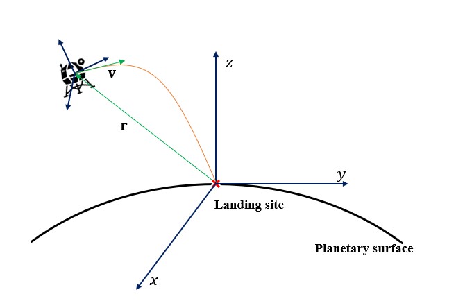
Figure 1: Spacecraft Landing Geometry

2 BACKGROUND AND PRELIMINARIES

2.1 Dynamics and Preliminary Results

The non-rotating inertial ENU-frame with origin at the landing site is considered as shown in Fig. 1. Assuming a 3-DOF dynamics in $\mathbb{R}^{3}$ domain, the lander can be modelled as:

$$\begin{array}[]{ll}&\dot{\mathbf{r}}=\mathbf{v}\\ &\dot{\mathbf{v}}=\mathbf{a}_{c}+\mathbf{g}+\mathbf{a}_{\mathrm{p}}\\ &{\mathbf{a}}=\frac{\mathbf{T}}{m}\\ &\dot{m}=-\frac{\|\mathbf{T}\|}{I_{\mathrm{sp}}g_{e}}\end{array}$$ (5)

where $\mathbf{r},\,\mathbf{v}$ represent the position and velocity of spacecraft, and $\mathbf{g}$ is the local gravity, and since the altitude at which the powered descent stage starts is much smaller than the radius of the planet, $\mathbf{g}=[0,0,-g]^{\mathrm{T}}$ is a valid assumption. The guidance command is represented by $\mathbf{a}_{c}$, $\mathbf{a}_{\mathrm{p}}$ is the net acceleration caused due to bounded perturbations (e.g. wind), $m$ is the lander’s mass, $I_{\mathrm{sp}}$ is the specific impulse, and $g_{e}$ is the gravitational acceleration of Earth.

The performance index $J=0.5\int_{t_{0}}^{t_{f}}\mathbf{a}^{\mathrm{T}}\mathbf{a}\,d\mathrm{t}$ was minimised in [6], subject to (5) and fixed final time $t_{f}$ with $\mathbf{a}_{\mathrm{p}}=0$, to derive the OGL as:

$$\mathbf{a}=\frac{6}{t_{\mathrm{go}}^{2}}\mathbf{ZEM}-\frac{2}{t_{\mathrm{go}}}\mathbf{ZEV}.$$ (6)

where $t_{\mathrm{go}}\triangleq t_{f}-t$ is the time-to-go and:

$$\begin{array}[]{ll}&\mathbf{ZEM}\triangleq{\mathbf{r}_{f}^{d}}-\left[\mathbf{r}(t)+\mathbf{v}t_{\mathrm{go}}+0.5\mathbf{g}t_{\mathrm{go}}^{2}\right]\\ &\mathbf{ZEV}\triangleq{\mathbf{v}_{f}^{d}}-\left[\mathbf{v}(t)+\mathbf{g}t_{\mathrm{go}}\right]\end{array}$$ (9)

here ${\mathbf{r}_{f}^{d}},\,{\mathbf{v}_{f}^{d}}$ represents desired position and velocity at $t_{f}$.

2.2 Optimal Terrain Avoidance Guidance Law

To avoid crashing in to the surface, the results in [6] were extended in [17, 18] by introducing a penalty term, which was a function of the distance of lander from the surface, to the standard performance index for fuel optimality. On the other hand, the idea of barriers were introduced in [12] to avoid more general terrain, however fuel optimality was not considered. A novel penalty to the performance index was introduced in [14], which was a function of the distance of lander with respect to the barriers, defined as $d_{i}\triangleq r_{i}-\rho_{i,j}$ where $i=x,\,y,\,z$. Here, predetermined terrain information can be used to approximate the terrain as $n$-step shapes and pre-define the barrier polynomials $\rho_{i,j}$ using the $n$-steps where $j$ is the counter for $n$-steps. An illustration of the barriers along with terrain approximated as $n$-step shapes is shown in Fig. 2. The figure also details the expressions used to create the barrier polynomials. The constants $\alpha_{i,j}$, $\beta_{i,j}$ and $\gamma_{i,j}$ are determined using the height and width of each step w.r.t the origin. Further details of the barrier formulation can be found in Section 3 of [14]. The modified performance index was considered as $J=0.5\int_{0}^{t_{f}}\big{[}\mathbf{a}^{\mathrm{T}}\mathbf{a}-\sum_{i}l_{3,i}e^{-\psi_{i}}\big{]}\,d\mathrm{\tau}$ where $e^{-\psi_{i}}$ is the augmentation term with $\psi_{i}\triangleq{l_{2,i}}/{(d_{i}^{2}+l_{1,i})}$, and here $l_{1,i},\,l_{2,i},\,l_{3,i}>0$ are constants.

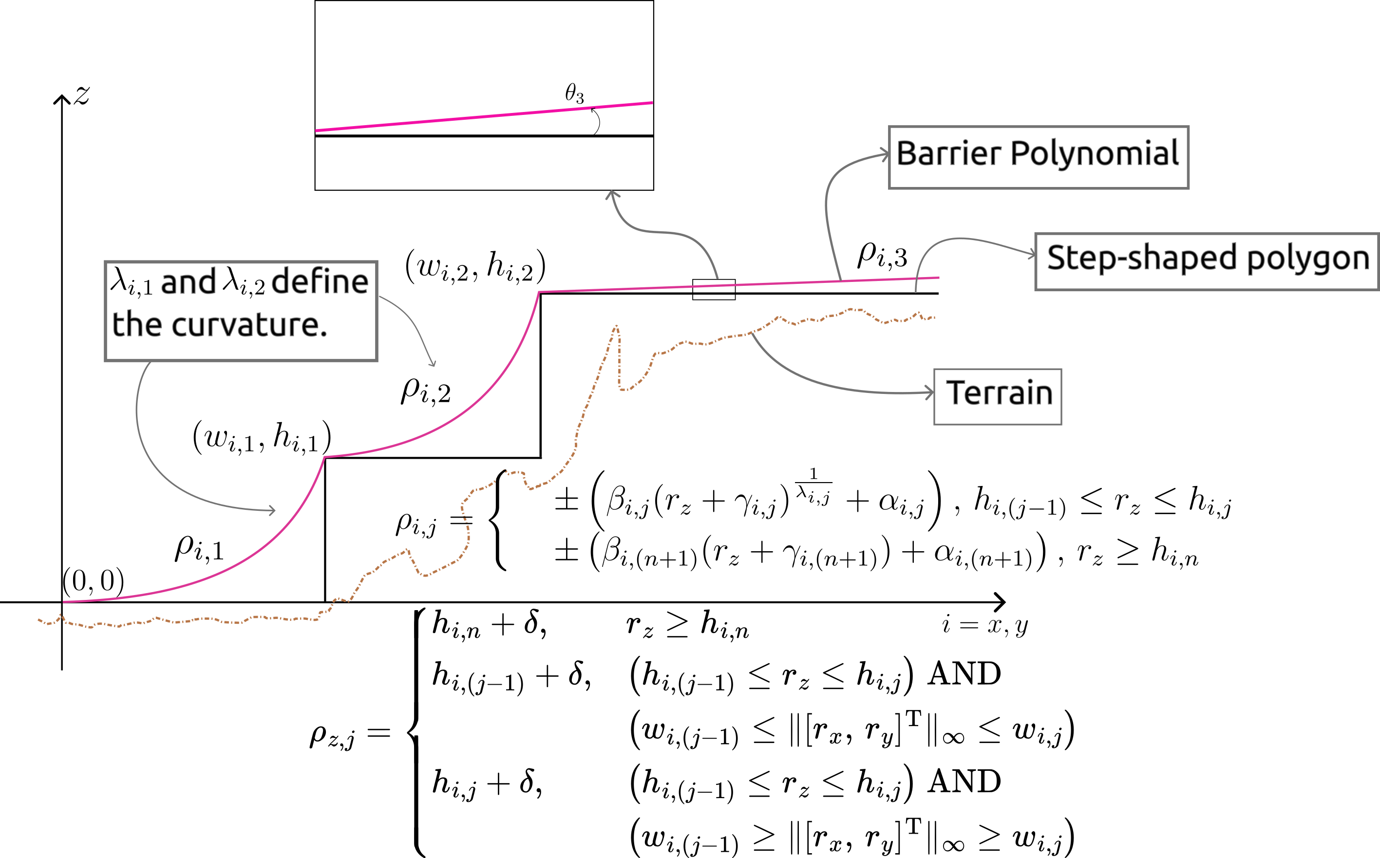
Figure 2: Illustration of barriers with $n=2$ [14]

Solving the minimum control effort problem, we get the near-fuel-optimal terrain avoidance guidance law as:

$$\mathbf{a}_{\mathrm{OTALG}}=\frac{6}{t_{\mathrm{go}}^{2}}\mathbf{ZEM}-\frac{2}{t_{\mathrm{go}}}\mathbf{ZEV}+\mathbf{p}\frac{t_{\mathrm{go}}^{2}}{12},$$ (10)

where $\mathbf{ZEM}$ and $\mathbf{ZEV}$ are as defined in (9). Comparing (6) and (10), $\mathbf{p}t_{\mathrm{go}}^{2}/12$ is responsible for the divert manoeuvre and $\mathbf{p}\triangleq[\dot{p}_{r_{x}},\,\dot{p}_{r_{y}},\,\dot{p}_{r_{z}}]$ where:

$$\dot{p}_{r_{i}}=l_{2,i}l_{3,i}\frac{d_{i}\mathrm{e}^{-\psi_{i}}}{(d_{i}^{2}+l_{1,i})^{2}}.$$ (11)

3 ROBUST OTALG USING MULTIPLE SLIDING SURFACES (MSS)

The OTALG presented in [14] showed good performance in terms of near-fuel-optimality and terrain avoidance compared to the existing literature. While OTALG is able to avoid the terrain with near-fuel-optimality, it was lacking in terms of accuracy of precision soft landing. Further, it was not designed to reject disturbances. Hence, expanding on the OTALG, multiple sliding surfaces are used here to improve its robustness and guarantee precision soft landing while having low fuel consumption even in the face of bounded external disturbances.

3.1 MSS Design: Surface 1

The first sliding surface is defined as $\mathbf{s}_{1}\triangleq\mathbf{r}-{\mathbf{r}_{f}^{d}}$ where ${\mathbf{r}_{f}^{d}}$ is the desired terminal position. This sliding surface is used to track the position error. To track $\mathbf{s}_{1}$ and drive the position error to zero, a virtual controller is defined as $\dot{\mathbf{s}}_{1}=-\frac{\Lambda}{t_{\mathrm{go}}}\mathbf{s}_{1}$ where $\Lambda>0$ is constant.

Theorem 1.

The virtual controller defined by $\dot{\mathbf{s}}_{1}=-\frac{\Lambda}{t_{\mathrm{go}}}\mathbf{s}_{1}$, is globally stable. Further, both $\mathbf{s}_{1}$ and its derivative, under the reaching law defined by the virtual controller reach zero in finite time.

Proof.   Global stability can be guaranteed for the virtual controller using Lyapunov’s second method, and choosing the candidate Lyapunov function as $V_{1}=0.5\mathbf{s}_{1}^{\mathrm{T}}\mathbf{s}_{1}$. From direct observation, it is clear that $V_{1}$ is positive definite everywhere, except at $\mathbf{s}_{1}=\mathbf{0}$ where $V_{1}(\mathbf{s}_{1}=\mathbf{0})=0$. Further, the candidate Lyapunov function is radially unbounded. To guarantee global stability, the time derivative of $V_{1}$ must be negative definite everywhere, that is $\dot{V}_{1}=\mathbf{s}_{1}^{\mathrm{T}}\dot{\mathbf{s}}_{1}<0$. This implies:

$$\dot{V}_{1} =-\frac{\Lambda}{t_{\mathrm{go}}}\mathbf{s}_{1}^{\mathrm{T}}\mathbf{s}_{1}<0$$ (12)

Equation (12) proves that the virtual controller is globally stable, and concludes the first part of the proof. To analyse the finite-time stability, we solve the differential equation given by the virtual controller component-wise.

$$\frac{\mathrm{d}s_{1i}}{\mathrm{dt}}=-\frac{\Lambda}{t_{\mathrm{go}}}s_{1i}$$

$$\Rightarrow \ln{s_{1i}}=\Lambda\ln{t_{\mathrm{go}}}+C_{1}$$

$$\Rightarrow \begin{array}[]{ll}s_{1i}=s_{1i0}\left({\frac{t_{\mathrm{go}}}{t_{f}}}\right)^{\Lambda}\\ \dot{s_{1i}}=-\frac{\Lambda}{t_{f}}s_{1i0}\left({\frac{t_{\mathrm{go}}}{t_{f}}}\right)^{\Lambda-1}\end{array}$$ (15)

The sliding surface and its derivative can be made finite-time convergent at $t=t_{f}$ by setting $\Lambda>1$, and thus concluding the proof of this theorem. $\Box$

3.2 MSS Design: Surface 2

At the beginning of powered descent stage, due to a variety of reasons, such as disturbances caused due to model uncertainty and atmospheric perturbations, the relation $\dot{\mathbf{s}}_{1}=-\frac{\Lambda}{t_{\mathrm{go}}}\mathbf{s}_{1}$ is not satisfied. The guidance law should be designed to drive $\dot{\mathbf{s}}_{1}$ from its initial condition to $\dot{\mathbf{s}}_{1}=-\frac{\Lambda}{t_{\mathrm{go}}}\mathbf{s}_{1}$, maintain it there regardless of any disturbances, and eventually drive $\mathbf{s}_{1}$ to zero. To achieve this, a second sliding surface is proposed as:

$$\mathbf{s}_{2}=\dot{\mathbf{s}}_{1}+\frac{\Lambda}{t_{\mathrm{go}}}\mathbf{s}_{1}$$ (16)

From $\mathbf{s}_{1}$ we have $\dot{\mathbf{s}}_{1}=\mathbf{v}-{\mathbf{v}_{f}^{d}}$ and $\ddot{\mathbf{s}}_{1}=\mathbf{a}_{c}+\mathbf{g}-\dot{\mathbf{v}}_{f}^{d}$, which when substituted in time derivative of (16) gives:

$$\dot{\mathbf{s}}_{2} =\ddot{\mathbf{s}}_{1}+\frac{\Lambda}{t_{\mathrm{go}}}\dot{\mathbf{s}}_{1}+\frac{\Lambda}{t_{\mathrm{go}}^{2}}\mathbf{s}_{1}$$

$$\dot{\mathbf{s}}_{2} =\mathbf{a}_{c}+\mathbf{g}-\dot{\mathbf{v}}_{f}^{d}+\frac{\Lambda}{t_{\mathrm{go}}}(\mathbf{v}-{\mathbf{v}_{f}^{d}})+\frac{\Lambda}{t_{\mathrm{go}}^{2}}(\mathbf{r}-{\mathbf{r}_{f}^{d}})$$ (17)

Since $\dot{\mathbf{s}}_{2}$, as shown in (17), has the acceleration term, the relative degree of $\mathbf{s}_{2}$ is 1, an appropriately chosen guidance law can drive $\mathbf{s}_{2}$ to zero.

Theorem 2.

Consider the system dynamics in (5) and the sliding surface $\mathbf{s}_{2}$ given by (16), the guidance law:

$$\mathbf{a}_{c}=\mathbf{a}_{\mathrm{OTALG}}-\bm{\Phi}\operatorname{sgn}{\mathbf{s}_{2}}-\mathbf{g}$$ (18)

where $\mathbf{a}_{\mathrm{OTALG}}$ is given by (10), will drive the second sliding surface $\mathbf{s}_{2}$ to zero in finite time, where $\bm{\Phi}=\mathrm{diag}\left\{\Phi_{x},\ \Phi_{y},\ \Phi_{z}\right\}$ is the sliding parameter, which depends on $d_{i}$ and $t_{\mathrm{go}}$.

Proof.   We begin the proof by choosing the candidate Lyapunov function as $V_{2}=0.5\mathbf{s}_{2}^{\mathrm{T}}\mathbf{s}_{2}$. From direct observation, $V_{2}$ is positive definite everywhere except at origin where it is zero and is radially unbounded everywhere in the domain of $\mathbf{s}_{2}$ that is $\mathbb{R}^{3}$. To prove global stability we analyse the negative definiteness of the time derivative of $V_{2}$, given by $\dot{V}_{2}=\mathbf{s}_{2}^{\mathrm{T}}\dot{\mathbf{s}}_{2}$. From (17) and (18), we get:

$$\dot{V}_{2} =\mathbf{s}_{2}^{\mathrm{T}}(\mathbf{a}_{\mathrm{OTALG}}-\bm{\Phi}\operatorname{sgn}{\mathbf{s}_{2}}-\dot{\mathbf{v}}_{f}^{d}+\frac{\Lambda}{t_{\mathrm{go}}}(\mathbf{v}-{\mathbf{v}_{f}^{d}})+\frac{\Lambda}{t_{\mathrm{go}}^{2}}(\mathbf{r}-{\mathbf{r}_{f}^{d}})).$$ (19)

From the nature of the landing guidance problem considered here, we have ${\mathbf{r}_{f}^{d}}=\mathbf{0}$ and ${\mathbf{v}_{f}^{d}}=\mathbf{0}$, and consequently $\dot{\mathbf{v}}_{f}^{d}=\mathbf{0}$. With these considerations, from (16), we have:

$$\mathbf{s}_{2}=\mathbf{v}+\frac{\Lambda}{t_{\mathrm{go}}}\mathbf{r}.$$ (20)

Then, from (9), (10) and (19), we get:

$$\dot{V}_{2}=\mathbf{s}_{2}^{\mathrm{T}}\bigg{[}\frac{\Lambda-6}{t_{\mathrm{go}}^{2}}\mathbf{r} +\frac{\Lambda-4}{t_{\mathrm{go}}}\mathbf{v}+\mathbf{p}\frac{t_{\mathrm{go}}^{2}}{12}-\bm{\Phi}\operatorname{sgn}\mathbf{s}_{2}\bigg{]}.$$ (21)

For $\Lambda=2,\,3$, from (20) and (21), we have:

$$\dot{V}_{2}=\frac{\Lambda-4}{t_{\mathrm{go}}}\mathbf{s}_{2}^{\mathrm{T}}\mathbf{s}_{2}+\mathbf{s}_{2}^{\mathrm{T}}\bigg{(}\mathbf{p}\frac{t_{\mathrm{go}}^{2}}{12}-\bm{\Phi}\operatorname{sgn}\mathbf{s}_{2}\bigg{)}.$$ (22)

We observe that the first term in (22), for $\Lambda=2,\,3$, is negative. To ensure the second term is negative as well, $\bm{\Phi}$ must be chosen suitably. Examining the second term component-wise for negative semi-definiteness, that is $s_{2i}\cdot\left(p_{i}\frac{t_{\mathrm{go}}^{2}}{12}-\Phi_{i}\operatorname{sgn}s_{2i}\right)\leq 0$. This implies,

$$s_{2i}\left(p_{i}\frac{t_{\mathrm{go}}^{2}}{12}\right) \leq\Phi_{i}|s_{2i}|$$

$$\Rightarrow\Phi_{i} \geq|p_{i}|\frac{t_{\mathrm{go}}^{2}}{12}.$$ (23)

Thus, setting $\Phi_{i}$ according to the inequality (23) will make (22) negative semi-definite and guarantee global asymptotic stability. Further, if the constraint on the sliding parameter in (23) is satisfied with strict inequality, then $\dot{V}_{2}$ will strictly be less than zero, and $V_{2}$ will converge to zero in finite time. Therefore, $\mathbf{s}_{2}$ also has finite time convergence, completing the proof for this theorem. $\Box$

3.3 Robustness Analysis

Now, we consider the disturbances in the environment, as expressed in (5), that can cause the spacecraft to deviate from its nominal trajectory. Equation (21) now becomes:

$$\dot{V}_{2}= \mathbf{s}_{2}^{\mathrm{T}}\left[\left(\frac{\Lambda-6}{t_{\mathrm{go}^{2}}}\mathbf{r}+\frac{\Lambda-4}{t_{\mathrm{go}^{2}}}\mathbf{v}\right)+\mathbf{a}_{\mathrm{p}}+\mathbf{p}\frac{t_{\mathrm{go}^{2}}}{12}-\bm{\Phi}\operatorname{sgn}\mathbf{s}_{2}\right]$$ (24)

Using a similar analysis used in the proof for Theorem 2, we get the following condition for guaranteed robustness:

$$\Phi_{i}\geq\left|p_{i}\frac{t_{\mathrm{go}}^{2}}{12}+a_{\mathrm{p}_{i}}\right|$$ (25)

where $a_{\mathrm{p}_{i}}$ is upper-bounded as $|a_{\mathrm{p}_{i}}|\leq a_{\mathrm{p}_{\mathrm{MAX}}}$.

4 ON THE CHOICE OF SLIDING PARAMETER

A common practice in sliding mode control is to fix the sliding parameter to be constant based on a-priori obtained estimates of disturbances. However, the lower bound on $\Phi_{i}$ defined in (25) depends on the states and the $t_{\mathrm{go}}$, and thus the sliding parameter should also be defined in the same manner. The maximum value of RHS in (25) can be determined and used as a sliding parameter, but it is an aggressive choice. An aggressive sliding parameter improves terminal precision as it commands a higher acceleration to turn towards the sliding surface as quickly as possible in the state-space and then maintain the states close to the sliding surfaces, requiring a higher control effort. Contrary to this, the states must come out of the vicinity of the sliding surface to avoid any collision with the terrain. To avoid aggressive sliding mode control and still achieve good accuracy in precision soft landing, we propose the sliding parameter as:

$$\Phi_{i}=k_{1}\left|p_{i}\right|\frac{t_{\mathrm{go}}^{2}}{12}+k_{2}a_{\mathrm{p}_{\mathrm{MAX}}}$$ (26)

where, $k_{1},\ k_{2}$ are tunable positive constants. Setting $k_{1},\,k_{2}=1$ guarantees (25) is satisfied. However, this requires divert manoeuvre to be executed with thrust higher than what is actually necessary. Setting $k_{1},\,k_{2}<1$ may, in fact, be sufficient to successfully execute the divert manoeuvre while still maintaining the robustness in precision soft landing. This, however, may lead to violations of (25), leading to loss of finite time stability and guaranteed robustness. We now show that even if the sliding constraint in (25) is violated, by choosing the sliding parameters as (26) with $k_{1},\,k_{2}<1$, the guidance law in (18) can still maintain robustness in precision soft landing. To this end, we first define the duration for which the dominant divert manoeuvre is active, and prove that the duration of the dominant divert manoeuvre is finite. Finally, we prove that with the sliding parameter chosen in (26), practical fixed time stability can be achieved.

Definition 1 (Duration of dominant divert manoeuvres).

Dominant divert manoeuvre is said to begin when $|p_{i}|t_{\mathrm{go}}^{2}/12>|(6/t_{\mathrm{go}}^{2})\mathrm{ZEM}_{i}-(2/t_{\mathrm{go}})\mathrm{ZEV}_{i}|$ and it ends when $|p_{i}|t_{\mathrm{go}}^{2}/12<|(6/t_{\mathrm{go}}^{2})\mathrm{ZEM}_{i}-(2/t_{\mathrm{go}})\mathrm{ZEV}_{i}|$. Further, in some cases when only a small divert acceleration is required, the dominant divert manoeuvre starts even with $|p_{i}|t_{\mathrm{go}}^{2}/12<|(6/t_{\mathrm{go}}^{2})\mathrm{ZEM}_{i}-(2/t_{\mathrm{go}})\mathrm{ZEV}_{i}|$ if $\operatorname{sgn}{\dot{d}_{i}}$ changes. In such cases, the dominant divert manoeuvre ends when $\operatorname{sgn}{\dot{d}_{i}}$ changes again.

Remark 1.

From the analysis of $p_{i}$ in Section 4.3 of [14], the behaviour of $|p_{i}|$ with respect to $d_{i}$ as shown in Fig. 3 is a decreasing function for all $|d_{i}|>|d_{i}^{*}|$ where $d_{i}^{*}$ is the value of $d_{i}$ for which $p_{i}$ is maximum, that is, $|p_{i}(d_{i}^{*})|=p_{\mathrm{MAX}}$. Also, note from the divert term in (10) and its definition in (11), for $d_{i}>0$ we have,

$$\frac{\partial(p_{i}t_{\mathrm{go}}^{2}/12)}{\partial d_{i}}= \Gamma\left[1-\frac{4d_{i}^{2}}{(d_{i}^{2}+l_{1,i})}+\frac{2l_{2,i}d_{i}^{2}}{(d_{i}^{2}+l_{1,i})^{2}}\right]\frac{t_{\mathrm{go}}^{2}}{12}.$$

where $\Gamma=\frac{l_{2,i}l_{3,i}e^{-\psi_{i}}}{(d_{i}^{2}+l_{1,i})^{2}}>0$ and $\frac{t_{\mathrm{go}}^{2}}{12}\geq 0$. The above expression can be then made negative for all values of $d_{i}>d_{i}^{*}$ by suitably choosing $l_{1,i}$ and $l_{2,i}$. This implies that when the lander approaches the barriers, that is, $d_{i}$ decreases, with initial conditions $d_{i}>d_{i}^{*}$, the divert term will necessarily increase and therefore will cause the dominant divert manoeuvre to begin. Similar logic also holds true for $d_{i}<0$.

Proposition 1.

The duration of a dominant divert manoeuvre is finite.

Proof.   Consider that the dominant divert manoeuvre begins for some $|d_{i}|>|d_{i}^{*}|$. During this time, the larger divert acceleration implies that the rate at which the lander approaches the barriers reduces. If the maximum thrust that the lander can generate is sufficiently large, then the sign of velocity, that is the direction of the velocity vector, will change and the lander will start to move away from the barrier. Observe that, in (10) when $t_{\mathrm{go}}$ is large and $|d_{i}|\gg|d_{i}^{*}|$, the magnitude of ZEM/ZEV component is of the order of $O(1/t_{\mathrm{go}}+g_{i})$, and when the $t_{\mathrm{go}}$ is small, the magnitude of ZEM/ZEV component is of the order of $O(1/t_{\mathrm{go}}^{2})$. Finally, for the mid-ranges of $t_{\mathrm{go}}$, the magnitude of ZEM/ZEV component has the order of $O(g_{i})$. Since initially $|d_{i}|\gg|d_{i}^{*}|$, $|p_{i}|t_{\mathrm{go}}^{2}/12\approx 0$. However, as $t$ increases, $t_{\mathrm{go}}$ decreases and $\lim_{t_{\mathrm{go}}\to 0}|p_{i}|t_{\mathrm{go}}^{2}/12=0$. This implies that at the end of the landing mission the magnitude of divert acceleration term in (10) comes sufficiently close to zero which is less than the magnitude of ZEM/ZEV term, and the dominant divert manoeuvre comes to an end in finite time. Since the mission is a fixed final time mission, this also implies that any dominant divert manoeuvre will come to an end in finite time. $\Box$

Figure 3: Behaviour of $p_{i}$ with respect to $d_{i}$ for $l_{1,i}=1,\,l_{2,i}=9500,\,l_{3,i}=500$.

Theorem 3.

The trajectory of the lander, governed by the dynamics given by (5) and under the guidance law $\mathbf{a}_{c}=\mathbf{a}_{\mathrm{OTALG}}-\bm{\Phi}\operatorname{sgn}\mathbf{s}_{2}-\mathbf{g}$ as defined in (18), have practical fixed-time stability (PFTS).

Proof.   From (22) we can obtain $\dot{V}_{2}=\sum\dot{V}_{2i},\>i=x,\,y,\,z$ where:

$$\dot{V}_{2i} =\left(\frac{\Lambda-4}{t_{\mathrm{go}}}\right)s_{2i}^{2}+s_{2i}\left(p_{i}\frac{t_{\mathrm{go}}^{2}}{12}-\Phi_{i}\operatorname{sgn}s_{2i}\right)$$

$$\Rightarrow\dot{V}_{2i} =A+B$$ (27)

where, $\mathrm{A}=\left({\Lambda-4}\right)\frac{|s_{2i}|^{2}}{t_{\mathrm{go}}}-\Phi_{i}|s_{2i}|$ and $\mathrm{B}=s_{2i}p_{i}\frac{t_{\mathrm{go}}^{2}}{12}$. Then, for $\Lambda=2,\,3$,

$$\mathrm{A}={2(\Lambda-4)V_{2i}}/{t_{\mathrm{go}}}-\sqrt{2}\Phi_{i}V_{2i}^{1/2}\leq-\sqrt{2}\Phi_{i}V_{2i}^{1/2}.$$ (28)

Similarly, for $B$, from Lemma 1:

$$\mathrm{B} =s_{2i}p_{i}\frac{t_{\mathrm{go}}^{2}}{12}$$

$$\Rightarrow\mathrm{B} \leq\left(\frac{2^{\frac{1+p_{1}}{2}}}{1+p_{1}}V_{2i}^{\frac{1+p_{1}}{2}}+\frac{p_{1}}{1+p_{1}}|p_{i}|^{\frac{1+p_{1}}{p_{1}}}\right)\frac{t_{\mathrm{go}}^{2}}{12}.$$ (29)

where $p_{1}>0$. Using (28) and (29) in (27), we get:

$$\begin{array}[]{lr}\dot{V}_{2i}&\leq-\bigg{(}\sqrt{2}\Phi_{i}V_{2i}^{1/2}-\frac{2^{\frac{1+p_{1}}{2}}}{1+p_{1}}V_{2i}^{\frac{1+p_{1}}{2}}\frac{t_{\mathrm{go}}^{2}}{12}\bigg{)}+\frac{p_{1}}{1+p_{1}}|p_{i}|^{\frac{1+p_{1}}{p_{1}}}\frac{t_{\mathrm{go}}^{2}}{12}\end{array}$$ (31)

Using the results of Lemma 2 in the Appendix (which gives the fundamental result on PFTS), we compare (31) with (42) to get

$$\begin{array}[]{rl}\alpha_{i}&=\sqrt{2}\Phi_{i}\\ \beta_{i}&=-\frac{2^{\frac{(1+p_{1})}{2}}}{1+p_{1}}\frac{t_{\mathrm{go}}^{2}}{12}\\ \eta_{i}&=\frac{p_{1}}{1+p_{1}}|p_{i}|^{\frac{1+p_{1}}{p_{1}}}\frac{t_{\mathrm{go}}^{2}}{12}\\ k=1,\>l=1/2,&m=\frac{(1+p_{1})}{2}\end{array}$$ (36)

where the conditions set by Lemma 2 enforce that $p_{1}>1$. Then, the settling time is given as:

$$T_{i}\leq\frac{2}{\sqrt{2}\Phi_{i}\theta}-\frac{2(1+p_{1})}{2^{\frac{p_{1}+1}{2}}(p_{1}-1)\theta}\frac{12}{t_{\mathrm{go}}^{2}}$$ (37)

where $i\>=\>x,\,y,\,z$. The RHS of (37) must be strictly positive and less than $t_{f}$, which lead to the following conditions respectively:

$$\Phi_{i} \leq\frac{2^{\frac{p_{1}}{2}}(p_{1}-1)}{1+p_{1}}\frac{t_{\mathrm{go}}^{2}}{12}=\mathrm{L}\>\text{(say)}$$ (38)

$$\Phi_{i} >\frac{1}{\frac{1+p_{1}}{2^{\frac{p_{1}}{2}}(p_{1}-1)}\frac{12}{t_{\mathrm{go}}^{2}}+\frac{t_{f}\theta}{\sqrt{2}}}=\mathrm{M}\>\text{(say)}.$$ (39)

In the condition given by (39), we observe that when $t_{\mathrm{go}}$ is large, $\Phi_{i}\geq M\approx\sqrt{2}/(t_{f}\theta)$, which can be satisfied by choosing a sufficiently large $a_{p_{\mathrm{MAX}}}$ in (26). Further, when $t_{\mathrm{go}}$ is very small, $\Phi_{i}\geq M\approx 0$ is trivially satisfied. Substituting the proposed sliding parameter (26) in (38) and rearranging the terms with $|p_{i}|=p_{\mathrm{MAX}}$, we get:

$$k_{1}p_{\mathrm{MAX}}+\frac{12k_{2}a_{\mathrm{p}_{\mathrm{MAX}}}}{t_{\mathrm{go}}^{2}}\leq\frac{2^{\frac{p_{1}}{2}}(p_{1}-1)}{(1+p_{1})}.$$ (40)

For all values of $t_{\mathrm{go}}\in(0,t_{f}]$, there exists a $p_{1}>1$ that satisfies (40). Further, in the condition given by (39), we observe that when $t_{\mathrm{go}}$ is large, $\Phi_{i}\geq M\approx\sqrt{2}/(t_{f}\theta)$, which can be satisfied by choosing a sufficiently large $a_{p_{\mathrm{MAX}}}$ in (26), and when $t_{\mathrm{go}}$ is very small, $\Phi_{i}\geq M\approx 0$ is trivially satisfied. Therefore, the proposed sliding parameter satisfies the conditions for PFTS set by (38) and (39), with settling time bounded by (37). Thus, even when the global finite time stability of Theorem 2 is not satisfied, the trajectories of the lander are PFTS, with settling time bounded by (37). $\Box$

5 SIMULATIONS AND DISCUSSIONS

5.1 Simulation Setup and Parameters

To demonstrate the effectiveness of MSS-OTALG, results from simulations are presented in this section. We assume a point-mass lander with specific impulse $I_{\mathrm{sp}}=225$ s, $T_{\mathrm{max}}=31000$ N. The value of $T_{\mathrm{max}}$ has been chosen based on the necessary condition derived in Section 4.3 of [14]. The desired terminal states are ${\mathbf{r}_{f}^{d}}=[0,\,0,\,0]^{\mathrm{T}}$ m, ${\mathbf{v}_{f}^{d}}=[0,\,0,\,0]^{\mathrm{T}}$ m/s, at terminal time $t_{f}=100$ s. The simulation is stopped when $r_{z}=0.05$ m or desired terminal time is achieved.

To emulate a trench surrounding the landing site on Mars, we consider the terrain that can be modelled as a $2$-step, flat-top shape (similar to the illustration in Fig. 2). The height and width of each step from the origin are given as $h_{i,i}=500,\,h_{i,2}=1000,\,w_{i,1}=600,\,w_{i,2}=1000$m. To design the barriers, we choose $\theta_{3}=0.05^{\circ}$, with $\lambda_{i,2}=6$, and $\lambda_{i,1}=20$. The guidance law constant are chosen as $l_{1,i}=1,\ l_{2,i}=9500,\$ and $l_{3,i}=500$, which gives the margin of safety for the vertical motion barrier as $\delta=1.2\cdot d_{i}^{*}=95.5$m. The local gravity at Mars is assumed to be $\textbf{g}=[0,\ 0,\,-3.7114]^{\mathrm{T}}$ m/s², and acceleration due to gravity on Earth $g_{e}=9.807$ m/s² [3]. Thruster actuation latency is incorporated as first-order delays as $\dot{\mathbf{a}}_{c}=(\mathbf{a}_{c_{\mathrm{ideal}}}-\mathbf{a}_{c})/\tau$ [10] where $\tau=0.0556$s to emulate 90% step response in 50ms [19]. In reality, the thrust commanded in never the exact thrust generated, especially in the case of solid rocket motors. To emulate this, we perturb the thrust command by $\pm 5\%$ using MATLAB’s rand() command. Finally, for sliding mode control we utilise $\Phi_{i}=k_{1}|p_{i}|{t_{\mathrm{go}}^{2}}/{12}+k_{2}a_{p_{\mathrm{MAX}}}$ where $k_{1}=0.8$ and $k_{2}=0.2$. To avoid the chattering problem associated with the signum function, we use the saturation function with boundary layer width $\epsilon=0.1$.

5.2 Illustration of a Numerical Example

Figure 4: Trajectory, velocity, commanded acceleration, divert term and sliding variables. [A: Divert manoeuvre 1 begins, B: Divert manoeuvre 1 ends, C: Divert manoeuvre 2 begins, D: Divert manoeuvre 2 ends]

To showcase the nominal performance of the proposed guidance law, the simulation results are presented in Figure 4. The initial conditions for this simulation are: ${\mathbf{r}_{0}}=[1051.86,\,562.15,\,2459.07]^{\mathrm{T}}$ m, ${\mathbf{v}_{0}}=[-165,\,-26.91,\,9.45]^{\mathrm{T}}$ m/s and $m_{0}=1905$ kg. From the trajectories, position, velocity and the commanded acceleration plots in Figs. 4a-d, it may be observed that the lander rises initially with a positive $v_{z}$ and then begins to descend at $t=4$s under the influence of gravity. During this time, to slow down the descent, a positive $a_{z}$ is continued to be commanded by the guidance law. Besides, note that a large and negative $v_{x}$ causes the lander to overshoot the desired landing site along the $x$-direction, which prompts the guidance law to generate a large and positive $a_{x}$ in order to slow down the lateral motion and bring the lander towards the landing site. As the lander nears the vertical motion barrier at $z=1000$m (refer to Figs. 4a-b), the first dominant divert manoeuvre begins at $t=40.2$s as the divert term surpasses the ZEM/ZEV term in the overall acceleration command (refer to (10), (18)), which is evident from Fig. 4e. As the vertical motion barrier is encountered, the divert acceleration and hence the commanded acceleration ramps up smoothly and does not exhibit discontinuities in the $a_{z}$ profile, which is justified from (11) and Fig. 3. Meanwhile, under the influence of positive $a_{x}$, the lander crosses the $x=-1000$m mark at $t=55.5$s. At this point, the vertical motion barrier switches from $\rho_{z,3}=1000+\delta$ to $\rho_{z,2}=500+\delta$. As a consequence, the magnitude of divert term falls below the magnitude of ZEM/ZEV term, and the first dominant divert manoeuvre comes to an end (refer to Fig. 4e). This also leads to the discontinuity observed in the $a_{z}$ profile at $t=55.5$s. On the other hand, the small discontinuities observed in the $a_{x}$ and $a_{y}$ profiles (refer to Fig. 4d) are due to $s_{2x}$ and $s_{2y}$ reaching nearly zero at around $t=65.8$s and $t=17.3$s, respectively, as can be seen in Fig. 4g. Those time-instants onwards, very small magnitude of $a_{x}$ and $a_{y}$ are only commanded to maintain $s_{2x}$ and $s_{2y}$, respectively, close to zero.

The effect of the divert term can also be observed in the sliding variables $s_{1z}$ and $s_{2z}$. Recall from (26) that the rate at which the $s_{2z}$ converges to zero is dependent on the choice of $k_{1}$ and $k_{2}$ in the sliding parameter. Larger values of of $k_{1}$ and $k_{2}$ imply that the convergence of $s_{2z}$ to zero is more aggressive. However, to execute the divert manoeuvre whenever necessary, smaller value of $k_{1}$ and $k_{2}$ are desirable in order to allow the state-space trajectory to leave the neighbourhood of the sliding surface $s_{2z}=0$. Hence, $k_{1}=0.8,\,k_{2}=0.2$ are chosen in this simulation.

Similar to the first divert manoeuvre, as observed from Fig. 4e, the second divert manoeuvre takes place when the lander approaches the last vertical motion barrier $\rho_{z,1}=\delta$ near the landing site. This slows down the lander further, thus further facilitating soft landing. However, the divert manoeuvre, in this case, ends soon due to small $t_{\mathrm{go}}$. However, when the lander crosses this barrier, the sign of divert term changes, as expected from its expression in (11). To avoid this behaviour, it is recommended that $\rho_{z,1}$ be sufficiently close to $r_{fz}^{d}$.

In this numerical example, there are two dominant divert manoeuvres. Since the number of divert manoeuvres is finite, and the sliding variables reach zero in finite time (see Figs. 4f-g), robustness of the MSS-OTALG is validated following the notion of PFTS in Theorem 3.

5.3 Comparative Simulation Study

Very few papers in existing literature have addressed both the problems of precision soft landing and terrain avoidance simultaneously. In this regard, it may be noted that it was stated in [10], a widely-referred precision soft landing paper, that the OSG presented therein could be augmented with the method in [17] for achieving precision soft-landing with terrain avoidance. This augmentation methods was later improved in [18]. Also, the MSS-OTALG presented in this paper is an expansion over the OTALG in [14], which also dealt with both these problems in an integrated way. Thus, in this section, the simulation study in Section 55.2 is extended to incorporate a comparative analysis of the performance of the MSS-OTALG w.r.t. that of the OTALG presented in [14] and augmented OSG [10, 18]. Illustrative examples of this comparative study using the same initial conditions and desired terminal condition, as in the previous subsection, under zero and non-zero atmospheric perturbation are presented in Figs. 5 (in Section 55.3.5.3.1) and 7 (in Section 55.3.5.3.2), respectively. Subsequently, extensive comparison study results under both zero and non-zero atmospheric perturbation are presented in Figs. 6 and 8, respectively.

5.3.1 Comparison study under zero atmospheric perturbations

Figure 5: Comparison of MSS-OTALG, aug. OSG and OTALG under no atmospheric perturbations.

Figure 6: MC simulation results for fuel consumption, landing dispersion and residual terminal velocity ($a_{\mathrm{P}}=0$). [1: MSS-OTALG, 2: augmented OSG, 3: OTALG]

From the trajectories in Fig. 5a, position profiles in Fig. 5b and velocity profiles in Fig. 5c, it is observed that all three guidance laws under comparison are able to drive the lander towards the desired landing site precisely and softly, while also successfully avoiding the terrain. From the net acceleration profile in Fig. 5e, observe that the augmented OSG applies a larger initial acceleration to bring the trajectory close to the sliding surface till $t=44.6$s and subsequently a nearly constant acceleration to maintain the trajectory near the sliding surface. However, as the augmented OSG has been formulated to avoid terrain only in the $z-$direction, it avoids the terrain only marginally in the $x-y$ direction, as can be observed in Fig. 5a. On the other hand, the OTALG is formulated to avoid the terrain in any direction. When the lander is away from any terrain, OTALG behaves similar to the OGL [6] in the sense that it applies just enough acceleration for precision soft-landing. But, when the terrain is encountered, the divert term starts to dominate the ZEM/ZEV term in the guidance law, leading to a higher acceleration commanded by OTALG to avoid the terrain and again bring it back to the desired landing site when the terrain is sufficiently avoided. The consequence of these two very different acceleration profiles is that while the augmented OSG has an excellent performance in terms of landing precision but the OTALG outperforms the former in terms of fuel consumption and terrain avoidance. Further, in the case of augmented OSG, increasing the sliding parameter to improve precision also increases the turn rate of the lander, which may be detrimental to the sensitive equipment carried onboard. To this end, the MSS-OTALG developed in this paper finds a middle ground between these conflicting objectives.

The presence of the sliding term in the MSS-OTALG imparts a high degree of precision, akin to the augmented OSG to the tune of $\Delta x_{f}=9.31\cdot 10^{-7}$m, $\Delta y_{f}=3.64\cdot 10^{-7}$m and $\Delta v_{zf}=-0.02$m/s for MSS-OTALG, $\Delta x_{f}=-9.98\cdot 10^{-6}$m, $\Delta y_{f}=3.45\cdot 10^{-6}$m and $\Delta v_{zf}=-0.01$m/s for augmented OSG and $\Delta x_{f}=-7.32\cdot 10^{-2}$m, $\Delta y_{f}=3.0\cdot 10^{-3}$m and $\Delta v_{zf}=-3.67$m/s for OTALG. Moreover, as the OTALG is also embedded in the formulation of MSS-OTALG, it inherits the feature of terrain avoidance in all directions and near-fuel-optimality from OTALG, which is evident from fuel consumption data ($\Delta m=391.37$ kg for MSS-OTALG, $\Delta m=394.60$ kg for aug. OSG and $\Delta m=379.22$ kg for OTALG). In this way, MSS-OTALG reconciles seemingly conflicting objectives, with both the sliding and divert terms collaborating to achieve terrain-avoided soft landing objectives.

Table 1: Normal Distribution for Initial Conditions

State	$x_{0}$	$y_{0}$	$z_{0}$	$v_{\mathrm{x0}}$	$v_{\mathrm{y0}}$	$v_{\mathrm{z0}}$	$m_{0}$
Mean	0	0	2500	0	0	-80	1905
SD	2200	2200	400	80	80	20	0

Monte Carlo simulations are conducted using 300 initial conditions selected from the normal distribution outlined in Table 1. The purpose is to objectively assess the soft-landing accuracy and fuel consumption statistics of the three guidance laws under comparison. The results of these simulations are depicted using box plot representation in Fig. 6, while the corresponding statistical data is summarised in Table 2. Augmented OSG and MSS-OTALG exhibit a high degree of accuracy in precision soft landing (refer to Fig. 6b-d), yet the former consumes significantly more fuel than the latter (as determined via paired t-test with null hypothesis $H_{0}:\Delta m_{\mathrm{aug.\,OSG}}=\Delta m_{\mathrm{{MSS-OTLAG}}}$ against $H_{1}:\Delta m_{\mathrm{aug.\,OSG}}>\Delta m_{\mathrm{{MSS-OTLAG}}}$, which gives $t_{\mathrm{stat}}=14.35$). This can also be observed from Fig. 6a. Conversely, OTALG is found to consume quite less fuel compared to MSS-OTALG, but performs poorly in terms of precision soft-landing performance. Thus, these Monte Carlo studies validate that the MSS-OTALG developed in this paper achieves significantly superior performance in precision soft-landing while also avoiding terrain yet demanding near-to-optimal fuel consumption.

Table 2: Terminal States Statistics ($a_{\mathrm{p}}=0$)

Guidance Law	Mean				SD
	$\Delta m$	$\Delta x$	$\Delta y$	$\Delta v_{z}$	$\Delta m$	$\Delta x$	$\Delta y$	$\Delta v_{z}$
MSS-OTALG	$366.67$	$1.65\cdot 10^{-5}$	$4.37\cdot 10^{-5}$	$-3.32\cdot 10^{-2}$	$12.72$	$6.25\cdot 10^{-4}$	$6.48\cdot 10^{-4}$	$8.29\cdot 10^{-2}$
aug. OSG	$371.73$	$1.67\cdot 10^{-6}$	$-1.55\cdot 10^{-5}$	$-6.69\cdot 10^{-2}$	$12.89$	$6.78\cdot 10^{-4}$	$6.19\cdot 10^{-4}$	$0.13$
OTALG	$365.91$	$-2.40$	$1.84$	$-7.43$	$19.62$	$46.29$	$31.23$	$4.22$

5.3.2 Comparison study under non-zero atmospheric perturbations

Figure 7: Comparison of MSS-OTALG, aug. OSG and OTALG under bounded atmospheric perturbations.

Figure 8: MC simulation results for fuel consumption, landing dispersion and residual terminal velocity ($a_{\mathrm{P}}\neq 0$). [1: MSS-OTALG, 2: augmented OSG, 3: OTALG]

Presence of disturbances, such as those caused due to atmosphere, can cause the lander to go off the nominal course and can cause the lander to perform poorly in terms of precision soft landing. In this section, comparative simulation study under non-zero atmospheric perturbations is presented in which $\mathbf{a}_{p}(t)=0.3\mathbf{a}_{c}\sin{\left({\pi t}/{3}\right)}$ is considered as the model for atmospheric perturbations. Using the same initial conditions as in Fig. 5, illustrative examples using the three guidance laws - MSS-OTALG, augmented OSG and OTALG - are presented in Fig. 7. All of them are able to avoid the terrain and precisely and softly land close to the desired landing site, as evident from Fig. 7a-c. Similar to the zero perturbation case, the augmented OSG demands a higher initial acceleration due to the sliding term, which in effect improves the disturbance rejection capability as can be observed in Fig. 7d-e, where the command acceleration and thrust vary to attenuate the disturbances caused by the winds. This results in almost no oscillations in the velocity of the lander, as can be observed in Fig. 7c. On the other hand, since the OTALG does not have any disturbance rejection capability, the thrust and commanded acceleration profiles are similar to that of zero perturbation case, however this causes the lander to sway continuously and thus degrade the soft-landing accuracy, as can be observed in the velocity profiles shown in Fig. 7c. Coming to the MSS-OTALG, sufficient disturbance rejection can be observed due to the sliding term, and at the same time the terrain is avoided due to the divert term. Since the constants $k_{1},\,k_{2}<1$ have been chosen for the sliding parameter, the disturbance rejection by MSS-OTALG is not as effective as that by the augmented OSG. However, it attenuates the disturbances caused by the wind significantly better that the OTALG. This phenomenon can be observed in the acceleration command and thrust profiles (refer to Fig. 7d-e). It can also be observed that as the divert term’s influence increases, it dominates the effect of the sliding term to avoid the terrain. Then, when the divert term is small the sliding term operates to mitigate disturbances, improving the accuracy of the precision soft landing.

To assess both the soft-landing precision and fuel usage in the presence of atmospheric disturbances, Monte-Carlo simulations has been conducted utilising the same 300 initial conditions as used in the Monte-Carlo simulations shown in Fig. 6. The outcomes are graphically represented via box plots in Fig. 8 and numerically summarised in Table 3. It’s evident from the simulations that the augmented OSG, as anticipated from the thrust and acceleration profiles in Fig. 7d-e, consumes more fuel. However, it consistently delivers the most accurate precision soft-landings. MSS-OTALG exhibits slightly higher fuel consumption compared to OTALG but, showcases commendable performance in precision soft-landing akin to the augmented OSG. On the other hand, although OTALG demonstrates lower fuel consumption compared to the augmented OSG and MSS-OTALG, it suffers from significantly poorer performance in precision soft-landing. Hence, the Monte-Carlo simulations effectively validate the robustness of MSS-OTALG in mitigating the impact of non-zero atmospheric perturbations while achieving the main objectives of terrain-avoided precision soft landing.

Table 3: Terminal States Statistics ($a_{\mathrm{p}}\neq 0$)

Guidance Law	Mean				SD
	$\Delta m$	$\Delta x$	$\Delta y$	$\Delta v_{z}$	$\Delta m$	$\Delta x$	$\Delta y$	$\Delta v_{z}$
MSS-OTALG	$367.73$	$2.75\cdot 10^{-5}$	$-4.71\cdot 10^{-5}$	$-0.17$	$11.74$	$1.37\cdot 10^{-3}$	$1.37\cdot 10^{-4}$	$4.49\cdot 10^{-2}$
aug. OSG	$381.33$	$3.03\cdot 10^{-5}$	$-9.02\cdot 10^{-5}$	$-0.19$	$12.46$	$1.05\cdot 10^{-3}$	$1.02\cdot 10^{-3}$	$0.15$
OTALG	$361.50$	$-1.87$	$1.41$	$-8.21$	$19.58$	$36.36$	$23.66$	$3.71$

6 CONCLUSION

Expanding upon the Optimal Terrain Avoidance Landing Guidance Law (OTALG) recently presented in literature with the help of sliding mode control by multiple sliding surfaces (MSS), a near-fuel optimal and robust guidance law for precision soft-landing in hazardous terrain, named MSS-OTALG, is presented in this paper. The incorporation of MSS renders it the desired robustness. To allow the lander to manoeuvre away from the terrain, a state and time-dependent sliding parameter is introduced, and practical fixed time stability is proven under the proposed guidance law. Finally, extensive computer simulations validate the ability of the MSS-OTALG to avoid the terrain and precisely and softly land at the desired landing site while having low fuel consumption, under realistic limitations posed by thruster dynamics, thrust constraints and atmospheric disturbances. When compared against the OTALG and an augmented version of optimal sliding guidance (OSG) using Monte Carlo simulations, it was observed that the MSS-OTALG finds the middle ground in terms of all the performance measures.

Appendix A Important Lemmas

Lemma 1.

(Young’s Inequality) For any vector $\mathbf{x}$, $\mathbf{y}\in\mathbb{R}^{n}$, $\mathbf{x}^{\mathrm{T}}\mathbf{y}\leq\|\mathbf{x}\|^{a}/a+\|\mathbf{y}\|^{b}/b$ holds true where $a,\,b>1$ and $(a-1)(b-1)=1$.

Lemma 2.

[15, 16] Consider the system,

$$\dot{\mathbf{x}}=\mathbf{f}(\mathbf{x}(t)),\>\mathbf{x}(t_{0})=\mathbf{x}_{0}.$$ (41)

Suppose there exists a Lyapunov function $V(\mathbf{x})$ such that,

$$\dot{V}(\mathbf{x})\leq-\left(\alpha V^{l}(\mathbf{x})+\beta V^{m}(\mathbf{x})\right)^{k}+\eta$$ (42)

where $\alpha$, $\beta$, $l$, $m$, $k$ $>0$, $lk<1$, $mk>1$ and $0<\eta<\infty$. Then the trajectories of (41) are practically fixed-time stable, with residual set

$$\left\{\lim_{t\rightarrow T}\mathbf{x}\left|\right.V(\mathbf{x})\leq\min\left\{\begin{array}[]{cc}&\alpha^{-\frac{1}{l}}\left(\frac{\eta}{1-\theta^{k}}\right)^{\frac{1}{lk}},\\ &\beta^{-\frac{1}{l}}\left(\frac{\eta}{1-\theta^{k}}\right)^{\frac{1}{mk}}\end{array}\right\}\right\}$$ (45)

where $\theta\in(0,1]$ and the settling time, $T$ is upper bounded by

$$T\leq\left(\frac{1}{\alpha^{k}\theta^{k}(1-lk)}+\frac{1}{\beta^{k}\theta^{k}(mk-1)}\right).$$ (46)

Throughout the paper the signum function, $\operatorname{sgn}(\cdot)$ is defined as:

$$\operatorname{sgn}\Delta\triangleq\left\{\begin{array}[]{cc}-1&\mathrm{if}\>\Delta<0\\ 0&\mathrm{if}\>\Delta=0\\ 1&\mathrm{if}\>\Delta>0\end{array}\right..$$ (47)

Further, consider $\mathbf{x}\in\mathbb{R}^{n}$, then

$$\operatorname{sgn}\mathbf{x}\triangleq\left[\operatorname{sgn}x_{1},\,\operatorname{sgn}x_{2},\dots,\operatorname{sgn}x_{n}\right]^{\mathrm{T}}.$$ (48)

References

- [1] NASA/JPL-Caltech, “Mars Probe Landing Ellipses.” [Online]. Available: https://www.jpl.nasa.gov/images/pia24377-mars-probe-landing-ellipses
- [2] B. Wu, J. Dong, Y. Wang, W. Rao, Z. Sun, Z. Li, Z. Tan, Z. Chen, C. Wang, W. C. Liu, L. Chen, J. Zhu, and H. Li, “Landing site selection and characterization of tianwen‐1 (zhurong rover) on mars,” Journal of Geophysical Research: Planets, vol. 127, no. 4, apr 2022.
- [3] B. Acikmese and S. R. Ploen, “Convex programming approach to powered descent guidance for mars landing.” Journal of Guidance, Control, and Dynamics, vol. 30, p. 1353–1366, 2007.
- [4] Y. Mao, M. Szmuk, and B. Açıkmeşe, “Successive convexification of non-convex optimal control problems and its convergence properties,” in 2016 IEEE 55th Conference on Decision and Control (CDC), 2016, p. 3636–3641.
- [5] B. S. Kim, J. G. Lee, and H. S. Han, “Biased PNG law for impact with angular constraint.” IEEE Transactions on Aerospace and Electronic Systems, vol. 34, p. 277–288, 1998.
- [6] B. Ebrahimi, M. Bahrami, and J. Roshanian, “Optimal sliding-mode guidance with terminal velocity constraint for fixed-interval propulsive maneuvers.” Acta Astronautica, vol. 62, p. 556–562, 2008.
- [7] R. Furfaro, B. Gaudet, D. R. Wibben, J. Kidd, and J. Simo, “Development of non-linear guidance algorithms for asteroids close-proximity operations.” in AIAA Guidance, Navigation, and Control (GNC) Conference, 2013.
- [8] R. Furfaro, D. Cersosimo, and D. R. Wibben, “Asteroid precision landing via multiple sliding surfaces guidance techniques.” Journal of Guidance, Control, and Dynamics, vol. 36, p. 1075–1092, 2013.
- [9] Y. Gong, Y. Guo, Y. Lyu, G. Ma, and M. Guo, “Multi-constrained feedback guidance for mars pinpoint soft landing using time-varying sliding mode,” Advances in Space Research, vol. 70, no. 8, p. 2240–2253, oct 2022.
- [10] D. R. Wibben and R. Furfaro, “Optimal sliding guidance algorithm for mars powered descent phase.” Advances in Space Research, vol. 57, p. 948–961, 2016.
- [11] C. Bai, J. Guo, and H. Zheng, “Optimal guidance for planetary landing in hazardous terrains,” IEEE Transactions on Aerospace and Electronic Systems, vol. 56, no. 4, p. 2896–2909, 2020.
- [12] Y. Gong, Y. Guo, G. Ma, Y. Zhang, and M. Guo, “Barrier lyapunov function-based planetary landing guidance for hazardous terrains.” IEEE/ASME Transactions on Mechatronics, vol. 27, p. 2764–2774, 2021.
- [13] ——, “Prescribed performance-based powered descent guidance for step-shaped hazardous terrains.” IEEE Transactions on Aerospace and Electronic Systems, vol. 58, p. 1083–1095, 2022.
- [14] S. Z. Basar and S. Ghosh, “Fuel-optimal powered descent guidance for hazardous terrain,” IFAC-PapersOnLine, vol. 56, no. 2, pp. 6018–6023, 2023, 22nd IFAC World Congress.
- [15] A. Polyakov, “Nonlinear feedback design for fixed-time stabilization of linear control systems,” IEEE Transactions on Automatic Control, vol. 57, no. 8, pp. 2106–2110, Aug. 2012.
- [16] B. Jiang, Q. Hu, and M. I. Friswell, “Fixed-time attitude control for rigid spacecraft with actuator saturation and faults,” IEEE Transactions on Control Systems Technology, vol. 24, no. 5, pp. 1892–1898, Sep. 2016.
- [17] L. Zhou and Y. Xia, “Improved ZEM/ZEV feedback guidance for mars powered descent phase.” Advances in Space Research, vol. 54, p. 2446–2455, 2014.
- [18] Y. Zhang, Y. Guo, G. Ma, and T. Zeng, “Collision avoidance ZEM/ZEV optimal feedback guidance for powered descent phase of landing on mars.” Advances in Space Research, vol. 59, p. 1514–1525, 2017.
- [19] M. Dawson, G. Brewster, C. Conrad, M. Kilwine, B. Chenevert, and O. Morgan, “Monopropellant hydrazine 700 lbf throttling terminal descent engine for mars science laboratory,” in 43rd AIAA/ASME/SAE/ASEE Joint Propulsion Conference and Exhibit. American Institute of Aeronautics and Astronautics, jul 2007.