The SIS process on Erdős-Rényi graphs: determining the infected fraction

Abstract

The SIS process on a graph poses many challenges. An important problem is to identify characteristics of the metastable behaviour. Existing mean-field methods (such as Heterogeneous Mean Field and the $N$-intertwined Mean Field Approximation) overestimate the metastable infected fraction, because they ignore correlations. Especially in sparse graphs, this leads to serious inaccuracies. We propose quenched and annealed methods incorporating correlations and giving significantly more accurate approximations. We use the Erdős-Rényi graph as a test case, but the methods can be generalized easily. Our methods are computationally very friendly and can be applied to fairly large graphs, in contrast with some other second-order mean field approximations.

Keywords: SIS process, Erdős-Rényi graph, Metastable behaviour, Infected fraction

1 Introduction

The Covid-19 virus was first identified in Wuhan (China) in December 2019, when it started to spread very quickly worldwide. In this initial stage, the number of cases was growing exponentially fast and the disease was disrupting society. In the next few years, many people got infected and there were several peaks of infections of the virus and its variants. Right now, it seems the situation is stabilizing. A large part of the world population has been infected at least once and many people have built up immunity. The number of new cases has dropped, but the disease still goes around and is expected to stay forever. The World Health Organization (WHO) shifts its focus from emergency response to long term Covid-19 disease management [20]. In this paper, we show how to predict and explain the behaviour of infectious diseases after stabilization.

Mathematical models for infectious diseases have been studied over the last decades, with a recently boosted interest due to the Covid-19 outbreak. In this work we focus on the SIS process (or contact process) on finite graphs. In this Markovian model, individuals are represented by nodes in a graph, which are either healthy or infected. Each infected node heals at rate 1, and it infects each of its healthy neighbors at rate $\tau$. This means that healthy individuals are always susceptible to the disease, like in the endemic Covid-19 phase. It motivates the terminology susceptible-infected-susceptible (SIS). For more background on the SIS process and related models, we refer to [16], [7].

The SIS process was first introduced by Harris [12] in 1974. Harris studied the process on the integer lattice $\mathbb{Z}^{d}$. It has later been studied on many other graphs [15, 17, 6, 23, 24], with recent attention to the process on random graphs [2, 4, 13, 18, 19]. Random graphs are designed to model social interactions within populations, and as such are suitable to model a population in which an infectious disease is spreading. Our focus in this paper is on the SIS process on Erdős-Rényi random graphs [9, 11]. For background on random graphs in general and the Erdős-Rényi graph in particular, we refer to [3, 25].

Our primary goal in this paper is to get a better understanding of the stabilized behaviour of the SIS-process on the Erdős-Rényi graph. Ultimately the process will reach the only stable solution in which all individuals are healthy. Assuming that the infection is strong enough to not dissappear immediately, extinction only happens at a very large time scale, see [4, 8, 10]. Before extinction, the process will be in a metastable or quasi-stationary state, which is quickly reached and corresponds to the Covid-19 endemic phase. We are particularly aiming at determining the infected fraction of the population in the metastable state based on the parameters of the process or on graph characteristics.

1.1 Review of models for the infected fraction

Exact analysis of the SIS process and its metastable state is hard, and only few rigorous results are available, even for quite simple graphs [6]. For a general graph given by its adjacency matrix, the probability distribution on the state space can in principle be computed numerically at any time. However, due to the exponential size of the state space, these matrix computations are limited to very small populations.

This is the reason that a lot of attention has gone to methods for approximating the behaviour of the process, see [21] for a discussion of the different approaches. Kephart and White consider the process on regular graphs, and derive a differential equation for the evolution of the infected fraction [14]. Wang et al. [27] had the interesting idea to generalize this to graphs with arbitrary adjacency matrix, but their results were shown to be inaccurate in the metastable regime [26]. This inspired Van Mieghem et al. [26] to introduce the $N$-intertwined Mean Field Approximation (NIMFA), which requires solving a system with ‘only’ $n$ unknowns to approximate the metastable infected fraction ($n$ being the population size). As the authors note, NIMFA overestimates the metastable infected fraction because it ignores correlations between nodes. As we will see, this is especially problematic if degrees in the graph are small. An attempt to correct NIMFA and take correlations into account is done in [5] with a second order approximation. Drawbacks are that it leads to a system with $n^{2}$ unknowns, and that its solutions might be unstable and physically meaningless.

The Heterogeneous Mean Field approximation (HMF) in [22] also implicitly ignores correlations.

One of our main findings is that simple averaging arguments are insufficient to get accurate predictions, especially when degrees in the graph are small. It is then important to take the exact degree distribution and correlations between nodes into account. We will present ways to do this and heuristics to accurately predict the infected fraction and related quantities. These methods are suitable to be applied beyond Erdős-Rényi graphs.

2 Preliminaries and goals

2.1 Model definitions

The goal of this paper is to predict and understand the behaviour of the contact process on Erdős-Rényi graphs. In particular we are interested in the quasi-stationary behaviour. Which fraction of the population will be infected on average if the process has reached its metastable equilibrium?

We denote the set of nodes in our Erdős-Rényi graph by $V=\{1,2,\ldots,n\}$. Each pair of nodes $\{i,j\}$ is connected (notation: $i\sim j$) with probability $p$, independent of all other pairs. This random graph is denoted $G_{n,p}$. We typically take $p$ to be a decreasing function of $n$. For instance, if $p=c/n$ for some constant $n$, the average degree does not depend on the size of the population. In this case $c$ has to be greater than 1, otherwise the graph only has small components which do not interact. If $c>1$, there is a unique giant component, containing a positive fraction of the population also for $n\to\infty$. The graph then is called supercritical. All Erdős-Rényi graphs in this paper are assumed to satisfy this criterion. Another threshold is $p=\log(n)/n$, when (almost) all nodes are in the giant.

On such an Erdős-Rényi graph $G=(V,E)$, we define our SIS process. This process is a continuous-time Markov process, with state space $2^{V}$. The state represents the set of infected nodes. Suppose $I\subseteq V$ is the set of infected nodes. The transition rates are then defined by

$$I\to I\setminus\{i\}\text{\ with\ rate\ $\delta$,\ for\ all\ }i\in I,$$ (healing)

$$I\to I\cup\{j\}\text{\ with\ rate\ }\#\{i\in I:i\sim j\}\cdot\tau,\text{\ for\ all\ }j\in V\setminus I.$$ (infection)

The healing rate for each infected node is $\delta$. Throughout this paper, we will stick to the convention that $\delta=1$, without loss of generality. The infection rate of an infected node to each of its healthy neighbors is $\tau$. Also for $\tau$, we will often take a function of $n$.

For each node $i$, we let $X_{i}(t)$ denote the status of node $i$ at time $t$, where $X_{i}(t)$ is either 1 (infected) or 0 (healthy). The total number of infected nodes at time $t$ is denoted by $X(t)$. Furthermore, we let

$$\overline{X}(t)=\frac{1}{n}\sum_{i=1}^{n}X_{i}(t)=\frac{X(t)}{n}$$

denote the infected fraction of the population at time $t$. Quasi-stationarity means that the probability distribution of these quantities is (almost) independent of $t$ in a large time window. Such behaviour will happen if the parameters admit a non-trivial state where healings and infections are balanced. For the complete graph, it is known that the quasi-stationary distribution is a well-defined object. This requires taking limits of $n$ and $t$ in the right way, see [1]. Similar behaviour is observed to appear in other graphs, in particular Erdős-Rényi graphs. Figure 1 clearly shows that the time evolution of the number of infected individuals fluctuates around some kind of equilibrium. In this paper we aim at predicting and understanding this equilibrium.

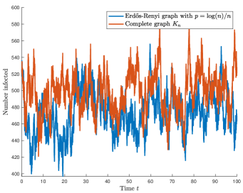
Figure 1: Number of infected nodes over time for the complete graph and an Erdős-Rényi graph. In both cases $n=1000$ and the effective infection rate $p\tau$ is equal to $2/n$, see the discussion in Section 2.2

2.2 A naive prediction for the infected fraction

The quasi-stationary distribution of the number of infected individuals is known for the contact process on the complete graph. Suppose the process has healing rate $1$ and infection rate $\tau=\lambda n^{-1}$ (for some constant $\lambda>1$). The number of infected nodes then has a normal (quasi-)stationary distribution with expectation $(1-\lambda^{-1})n$ and variance $\lambda^{-1}n$, see [1]. This result can be used for a first naive prediction for the metastable infected fraction in an Erdős-Rényi graph.

Consider the contact process with infection rate $\tau$ on the Erdős-Rényi graph $G_{n,p}$. An infected node can only infect a healthy node if there is an edge between them. Now assume that the event of two nodes being connected is independent of the event that exactly one of them is infected. The product $p\tau$ could then be interpreted as the expected infection rate between a random infected and a random healthy node and will be called the effective infection rate of the process. Heuristically, the behaviour on an Erdős-Rényi graph with edge probability $p$ and infection rate $\tau$ should be comparable to the behaviour on the complete graph with the same effective infection rate. To guarantee that the infected fraction of the population stays away from 0 and 1, we take $p\tau$ of order $n^{-1}$ so that we can write $p\tau=\lambda n^{-1}$ for some constant $\lambda>1$. Based on the heuristic that the effective infection rate determines the quasi-stationary infected fraction, comparison with the complete graph (which is $G_{n,p}$ with $p=1$) gives the following prediction

Heuristic 1.

Consider the contact process on an Erdős-Rényi graph $G_{n,p}$ with effective infection rate $p\tau=\lambda n^{-1}$. The quasi-stationary distribution satisfies

$$X\sim N(\mu,\sigma^{2}),\qquad\text{with}\qquad\mu=\left(1-\frac{1}{\lambda}\right)n,\qquad\sigma^{2}=\frac{n}{\lambda}.$$

We could make this into a heuristic for the infected fraction, by dividing by $n$. This gives

$$\overline{X}\sim N\left(1-\frac{1}{\lambda},\frac{1}{n\lambda}\right),$$

so the infected fraction converges to $1-\frac{1}{\lambda}$ if $n\to\infty$. The comparison with the complete graph only makes sense if the random graph is (almost) connected, i.e. the number of nodes outside the giant component should be negligible compared to $n$. This is equivalent to the number of isolated nodes being negligible [25]. For $p=\log(n)/n$, the expected number of isolated nodes is close to 1 for $n\to\infty$. So we should take $p$ at least of this order. For practical reasons, in our simulations we will mostly restrict to the case $\lambda=2$. We think that other choices give qualitatively similar behaviour.

To assess Heuristic 1, we did a simulation of the SIS process on the Erdős-Rényi graph with $n=1000$, $p=\log(n)/n$ and $\lambda=\tau np=2$ for $t\in[0,100]$. Heuristic 1 predicts that on average half of the population will be infected in the quasi-stationary situation. To get quick convergence to quasi-stationarity, we take each node to be infected with probability $1/2$ independently at $t=0$. We also did the simulation on the corresponding complete graph, so again with $\lambda=2$. Figure 1 shows the time evolution of the two processes.

Taking the average over time, the process on the complete graph has half of the population infected (this has been rigorously proved in [1]). Apparently, the average infected fraction in this realization of the Erdős-Rényi graph is lower, the picture shows an average around 470. Since we look at random graphs, the average infected fraction depends on the graph and might be different if we generate a new Erdős-Rényi graph. It could still be that the heuristic works well if we would average over multiple realizations of the Erdős-Rényi graph. We therefore repeated the simulation and generated 10 independent realizations of the Erdős-Rényi graph (all with $n=1000$ and $p=\log(n)/n$). On each of these graphs, we simulated the contact process with effective infection rate $p\tau=2/n$ for $0\leq t\leq 1000$. See Figure 2 for the (approximated) quasi-stationary distribution for each of the graphs and a comparison with the quasi-stationary distribution of the complete graph.

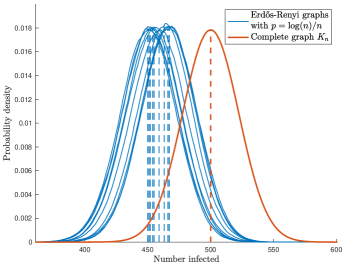
Figure 2: Probability distribution of the number of infected nodes in the complete graph (red) and in 10 realizations of the Erdős-Rényi-graph (blue), all with effective infection rate $2/n$. Dashed lines indicate means.

Based on Figure 2, there seems to be a systematic error in Heuristic 1, which does not vanish if we would average over multiple realizations of the Erdős-Rényi graph. The mean of the quasi-stationary distribution is typically smaller than $n/2$. Apparently Heuristic 1 is too naive. One reason is that the infected set is not a uniform selection of nodes. This is an essential difference with the complete graph, where transition rates only depend on the size of the infected set, not on the exact selection of infected nodes. In Erdős-Rényi graphs, nodes with higher degrees are more likely to be in the infected set. Another point is that there are local effects: neighbors tend to be infected or healthy simultaneously. These differences make the model more realistic, but at the same time more complicated. We can not just take averages over all nodes as in the complete graph, but need more subtle prediction methods.

2.3 Annealed and quenched predictions

When looking at Figure 2, we see that the distribution in the Erdős-Rényi graph is not only clearly different from the complete graph, but also depends on the realization of the graph. For a given graph $G$, we can estimate the metastable distribution by simulating the SIS process on this particular graph. The corresponding random variable depends on $G$ and on the infection rate $\tau$ and is denoted $X(G,\tau)$. Given $G$, the metastable mean infected number is a constant $\mu(G,\tau):=\mathbb{E}[X(G,\tau)\mid G]$. The expectation is taken with respect to the randomness of the process, not of the graph. We will call $\mu(G,\tau)$ the quenched mean and $\mu(G,\tau)/n$ the quenched infected fraction. Each blue curve in Figure 2 has its own quenched mean. Similarly, we denote the quenched variance by $\sigma^{2}(G,\tau)$.

If we take the graph to be random, then $\mathbb{E}[X(G,\tau)]$ becomes a random variable. Now we can take the expectation over the randomness of the graph as well to find the constant $\mathbb{E}[\mathbb{E}[X(G,\tau)]]$. This is what we will call the annealed mean. The annealed mean is independent of the graph realization and can be simulated by generating a bunch of graphs, running the process on each of them and taking the average of their metastable quenched means. For the SIS process on Erdős-Rényi graphs, the annealed mean is a function of the parameters which we denote by $\mu(n,p,\tau)$.

This gives rise to two different questions concerning prediction of the metastable infected fraction (or other quantities) in $G=G_{n,p}$:

1. Annealed prediction: given $n$, $p$ and $\tau$, predict $\mu(G,\tau)$, without observing $G$. The prediction will be a function $\hat{\mu}(n,p,\tau)$.

2. Quenched prediction: given the realization of $G$, predict $\mu(G,\tau)$ using the graph information. The prediction will be a function $\hat{\mu}(G,\tau)$.

When doing quenched prediction, we are estimating the constant $\mu(G,\tau)$. The metastable infected fraction is some complicated function of $G$ and $\tau$ which in principle could be determined exactly. However, when doing an annealed prediction, the realization of $G$ is not known and $\mu(G,\tau)$ is a random variable. This means that we will always make errors caused by the variation of this random variable. It therefore makes sense to investigate the order of the variance of $\mu(G,\tau)$ when $G$ is random.

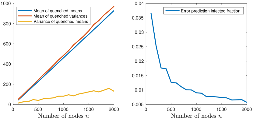
Figure 3: Left: Fixing an Erdős-Rényi graph, the metastable number of infected has mean (blue) and variance (red) both close to $n/2$. Varying the graph, the means themselves also fluctuate with a variance of order $n$ (yellow). Right: Approximate minimal standard error for any annealed method to predict a quenched infected fraction.

To do this, we generated for different values of $n$, realizations $G_{n}^{(1)},\ldots,G_{n}^{(100)}$ of an Erdős-Rényi graph $G_{n,p}$ with edge probability $p=\log(n)/n$. On each of them, we simulated the quenched mean $\mu(G_{n}^{(k)},\tau)$ and quenched variance $\sigma^{2}(G_{n}^{(k)},\tau)$ of the metastable distribution of the process with $\lambda=2$. Then we took averages over $k$ to obtain the mean of quenched means and the mean of quenched variances. Plotting them (Figure 3, left) shows that quenched means and quenched variances both grow linearly in $n$. In fact they are both close to $n/2$, as could be expected by comparing to the complete graph (cf. Heuristic 1).

Important is that also the variance of the quenched means appears to grow linearly with $n$. This means that annealed estimates for $\mu(G,\tau)$ will always have errors of the same order as fluctuations in the metastable distribution (i.e. the square root of the quenched variance). Therefore, graph information is for all graph sizes of significant importance to make accurate predictions. Taking the square root of the variance of the quenched means and dividing by $n$ gives the standard deviation in annealed prediction of $\mu(G,\tau)$, see right plot in Figure 3. For instance, for $n=1000$, the standard deviation is about 0.01. This means that any annealed estimation method for the infected fraction will make errors of at least this order.

This point is once again illustrated in Figure 4. Here we see simulations of infected fractions in Erdős-Rényi graphs of size $n=1000$ for different values of $p$. The simulation is compared with different heuristic predictions (all to be explained later in the paper). The point now is that some of these predictions are annealed (corresponding to the smooth curves) and some of them are quenched (the non-smooth curves). The quenched predictions fluctuate much more, but follow the simulation result much better. An annealed prediction can never predict these fluctuations, because they are caused by the randomness of the graph. Another noticable point is that Heuristic 1 systematically overestimates the infected fraction, especially when degrees are small.

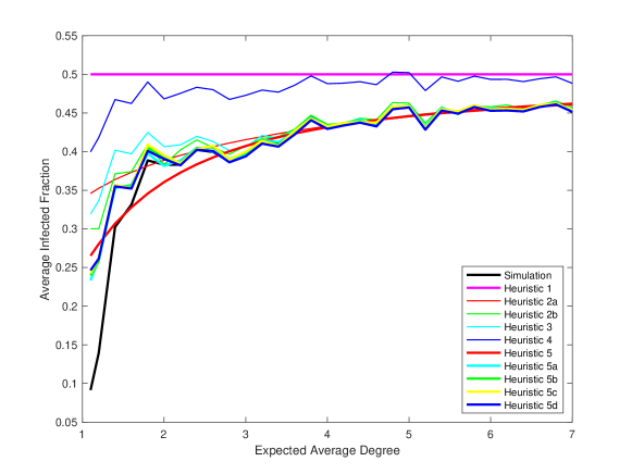
Figure 4: Simulated infected fraction compared to different predictions. In all cases, $n=1000$. The horizontal axis shows the expected average degree $np$.

The results of this paper are illustrated with extensive simulations and motivated by mathematical arguments. The main results include:

1. Quenched and annealed prediction methods for the metastable infected fraction in Erdős-Rényi graphs.

2. Degree-dependent predictions for the fraction of time individual nodes are infected.

3. Explanations why Heuristic 1 is flawed and how to repair these errors.

4. Degree-dependent predictions for correlations between neighboring nodes.

5. A heuristic to predict the metastable infected fraction in sparse graphs with other degree degree distributions, for which the giant component of $G_{n,p}$ is a test case.

An important point to take away is that it gets more and more delicate to make accurate predictions when graphs get sparser. Sparseness makes averages less reliable, correlations more important and heuristics more sensitive to errors. This can also be seen in Figure 4.

3 Improved heuristics for the infected fraction

When predicting the metastable infected fraction in an Erdős-Rényi graph, the graph structure and in particular the degree distribution is of key importance. In this section we show how to use the degrees to design more accurate prediction methods. One of these methods will turn out to be equivalent to NIMFA.

The methods in this section, although much better than Heuristic 1, still have their shortcomings. We will explain where it goes wrong, and in particular why NIMFA has a serious bias. Nevertheless, the ideas in this section are the basis for the exposition of more sophisticated methods in Section 4.

3.1 Nodes with higher degree are more frequently infected

Both in the Erdős-Rényi graph and in the complete graph, the fraction of nodes that is infected is close to $1-\lambda^{-1}$ and is quite stable over time, see again Figure 1. This also means that on average nodes are infected about a fraction $1-\lambda^{-1}$ of time.

Since nodes are indistinguishable in the complete graph, each individual node is expected to be infected the same fraction of time. In the complete graph ($n=1000,\lambda=2$), all nodes are infected about half of the time. If we send the running time (not too fast, to avoid extinction) and the number of nodes to infinity, this fraction of time will converge to 1/2 for each individual node. To illustrate, we ran the process on the complete graph for $10^{5}$ units of time and found that 99% of the nodes was infected between 49.5 and 50.3% of the time.

The fraction of time an individual node is infected could be quite different in the Erdős-Rényi graph. In Figure 5, we see a histogram of these fractions of time and an estimate of the density function (using kernel density estimation). In this Erdős-Rényi graph ($n=1000,p=\log(n)/n,\lambda=2$), nodes are only on average infected about half of the time. The fraction of time an individual node is infected ranges from 0 to about 0.7. For each individual node it will converge if the running time of the process increases, but the limiting fraction for each node will depend on the geometry of the graph.

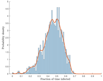
Figure 5: Simulated and estimated probability density of the fraction of time a node is infected.

The degree of a node can be used to give quite a good prediction for the fraction of time this node will be infected. This in turn will explain the shape of the density function in Figure 5. In first approximation, the fraction of time a randomly picked node is infected is equal to $1-\lambda^{-1}$. It therefore infects each of its neighbors at rate

$$\tau-\frac{\tau}{\lambda}.$$

Let $i$ be a random node with degree $d=d_{i}$. The fraction of time this node is infected will be called $f_{i}$. Assume that its neighbors are ‘random’ nodes. Then $i$ is healing at rate 1 and, since it has $d$ neighbors, getting infected at rate

$$d\tau-\frac{d\tau}{\lambda}.$$

If we consider a Markov process with one node, which is healing at rate 1 and getting infected at rate $\alpha$, in the stationary distribution this node is infected a fraction $\alpha/(1+\alpha)$ of time. Therefore, in our more complicated model, the fraction of time $i$ is infected can be estimated by

$$\hat{f}_{i}:=\frac{d\tau-\frac{d\tau}{\lambda}}{1+d\tau-\frac{d\tau}{\lambda}}.$$ (1)

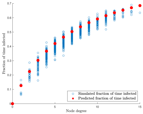
Figure 6: Simulation of the fraction of time nodes are infected, plotted as points $(d_{i},f_{i})$ in blue. The red markers indicate the degree-dependent prediction $(d,f_{d})$ based on the heuristic (1).

Fixing the parameters of the graph and the process, this estimate only depends on $d$, so we write $f(d)$ for $\hat{f}_{i}$. In Figure 6, we plotted the points $(d,f(d))$ and compare with all the points $(d_{i},f_{i})$ obtained by simulation of the contact process on an Erdős-Rényi graph ($n=1000,p=\log(n)/n,\lambda=2$).

In Figure 7, we compare the empirical distribution function of the per-node infected fraction of time,

$$\frac{1}{n}\sum_{i=1}^{n}\mathbbm{1}\left\{f_{i}\leq x\right\},$$

with the quenched estimated cumulative distribution function

$$\frac{1}{n}\sum_{i=1}^{n}\mathbbm{1}\{f(d(i))\leq x\}.$$

To compute this estimation, we need the actual degrees in the graph. Since we know that the degree distribution $D$ in the graph is $\text{Bin}(n-1,p)$, we can also estimate the distribution without observing the actual degrees by

$$\frac{1}{n}\sum_{i=1}^{n}\mathbbm{1}\{f(d(i))\leq x\} =\sum_{d=0}^{n-1}\frac{\#\{i:d_{i}=d\}}{n}\cdot\mathbbm{1}\{f(d)\leq x\}$$ (2)

$$\approx\sum_{d=0}^{n-1}\mathbb{P}(D=d)\cdot\mathbbm{1}\{f(d)\leq x\}$$ (3)

$$=\sum_{d=0}^{n-1}\binom{n-1}{d}p^{d}(1-p)^{n-1-d}\cdot\mathbbm{1}\{f(d)\leq x\}.$$ (4)

This prediction as well is compared with the observed empirical distribution in Figure 7. Note that this is an annealed prediction: it can be computed using only the three parameters $n$, $p$ and $\tau$.

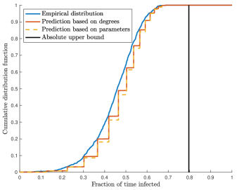
Figure 7: Cumulative distribution of infected fraction of time. Blue: empirical. Red: quenched prediction. Green: annealed prediction. Both predictions have jumps at the values $f(d)$. Black: absolute upper bound for the infected fraction caused by the maximal degree.

If the maximal degree $\Delta$ in the graph is known, we can compute an absolute upper bound for the (limiting) fraction of time a node is infected. Let $\theta$ be the maximal fraction of time a node is infected. Let $i$ be a node in the graph. If all its neighbors are infected all the time, then $i$ is infected at rate at most $\Delta\tau$. It follows that

$$\theta\leq\frac{\Delta\tau}{1+\Delta\tau}<1.$$ (5)

A sharper heuristic upper bound is obtained by the plausible assumption of positive correlations between $i$ and its neighbors. The neighbors of $i$ also are infected at most a fraction $\theta$ of time. Positive correlations mean that this upper bound still holds when restricting to periods when $i$ is healthy. Therefore, $i$ is infected at rate at most $\Delta\tau\theta$. This implies that

$$\theta\leq\frac{\Delta\tau\theta}{1+\Delta\tau\theta}.$$ (6)

It follows that $\theta$ is at most equal to the largest solution of (6), which is given by

$$\frac{\tau\Delta-1}{\tau\Delta}.$$

In our example in Figure 7, we have $\tau=2/(np)=2/\log(1000)\approx 0.29$ and $\Delta=17$. This gives approximately $0.79$ as an absolute upper bound for the fraction of time a node can be infected, see the vertical line in the plot.

Note that $\Delta=n-1$ in the complete graph $K_{n}$, giving the upper bound $1-1/((n-1)\tau)\approx 1-1/\lambda$. This is consistent with known results for $K_{n}$, see [1].

3.2 Degree-based heuristics for the infected fraction

The idea of estimate (1) will be used to predict the infected fraction $\mu/n=\mathbb{E}{\overline{X}}$ of the population. In the previous section, we estimated $\mu/n$ by $1-\lambda^{-1}$, based on Heuristic 1. We will derive a heuristic equation for $\mu/n$, leading to an improved estimate. Let $i$ be a node with degree $d$ and assume that its neighbors are infected a fraction $\mu/n$ of time. Analogous to (1), we estimate the fraction of time $i$ is infected by

$$\hat{f}_{i}:=\frac{d\tau\mu/n}{1+d\tau\mu/n}.$$ (7)

Averaging this quantity over all nodes in the graph, we obtain an estimate for $\mu/n$. Hence, if $n$, $p$ and $\tau$ are given, $\mu/n$ can be predicted by (numerically) solving

$$\frac{\mu}{n} =\frac{1}{n}\sum_{i=1}^{n}\hat{f}_{i}$$ (8)

$$=\sum_{d=0}^{n-1}\frac{\#\{i:d_{i}=d\}}{n}\cdot\frac{d\tau\mu/n}{1+d\tau\mu/n}$$ (9)

$$\approx\sum_{d=0}^{n-1}\binom{n-1}{d}p^{d}(1-p)^{n-1-d}\cdot\frac{d\tau\mu}{n+d\tau\mu}.$$ (10)

In fact the right hand side is the expectation $\mathbb{E}[\tau\mu D/(n+\tau\mu D)]$. Therefore, by Jensen’s inequality, (10) implies

$$\frac{\mu}{n}\leq\frac{\tau\mu\mathbb{E}[D]}{n+\tau\mu\mathbb{E}[D]}.$$ (11)

Solving for $\mu/n$ gives $\mu/n\leq 1-1/\lambda$, so that this procedure to predict the infected fraction always gives a lower estimate than Heuristic 1.

For large $n$ and $d$, the binomial probabilities in (10) are hard to compute, but they are well approximated by using the central limit theorem,

$$\mathbb{P}(\text{Bin}(n- 1,p)=d)\approx\mathbb{P}\left(|N((n-1)p,(n-1)p(1-p))-d|\leq\tfrac{1}{2}\right)$$ (12)

$$=\Phi\left(\frac{d-(n-1)p+\tfrac{1}{2}}{\sqrt{(n-1)p(1-p)}}\right)-\Phi\left(\frac{d-(n-1)p-\tfrac{1}{2}}{\sqrt{(n-1)p(1-p)}}\right),$$ (13)

where $\Phi$ is the cumulative distribution function of the standard normal. This gives us

Heuristic 2.

Consider the contact process on an Erdős-Rényi graph $G=G_{n,p}$ with infection rate $\tau$. The quasi-stationary infected fraction $\mu$ satisfies

$$\frac{\mu}{n}=\sum_{d=0}^{n-1}P(n,p,d)\cdot\frac{d\tau\mu}{n+d\tau\mu}.$$ (14)

Here $P(n,p,d)$ is either

1. The probability $\mathbb{P}(\text{Bin}(n-1,p)=d)$ or an approximation to it.

2. The exact frequency $\#\{i:d_{i}=d\}/n$.

Note that (a) gives an annealed prediction, while (b) is a quenched prediction. In view of earlier discussions, we expect (b) to be more accurate.

For $n\to\infty$, the probability mass of the degree distribution concentrates around its expectation $np$ with standard deviation $\sqrt{np(1-p)}$. This means that for $np\to\infty$ and $\tau np=\lambda$ the right hand side of (14) converges to

$$\lim_{n\to\infty}\frac{np\tau\mu}{n+np\tau\mu}=\frac{\lambda\lim_{n\to\infty}\mu/n}{1+\lambda\lim_{n\to\infty}\mu/n}.$$

Solving (14) for $\lim_{n\to\infty}\mu/n$, we obtain

$$\lim_{n\to\infty}\frac{\mu}{n}=1-\frac{1}{\lambda},$$ (15)

so that both versions of Heuristic 2 coincide with Heuristic 1 for $n\to\infty$. The advantage of taking $P(n,p,d)$ as a probability (as in Heuristic 2a) is that we do not need to know degrees in the graph.

3.2.1 Simulation and annealed prediction for $p=\log(n)/n$

We test Heuristic 2a, taking edge probability $p=\log(n)/n$ and using the normal approximation (13). The average degree in the graph is then about $\log(n)$, which is just enough to get an (almost) connected graph. For each $n=\lceil e^{k/10}\rceil$, $k=45,46,\ldots,80$, we generate 25 replications of the Erdős-Rényi graph so that in total we have $900$ graphs. The average degrees vary from $4.5$ to 8 and the sizes range from 91 to 2981 nodes. On each of those graphs, we simulate the contact process with infection rate $\tau=2/\log(n)$. With these choices, the effective infection rate is $\lambda=2$, so the crude Heuristic 1 predicts that on average half of the population is infected. Our simulation results are given in Figure 8. Each simulated graph is represented by a small blue circle. The horizontal coordinate is the expected average degree $\log{n}$. The vertical coordinate is the simulated infected fraction $\overline{X}$, averaged over time. This means it is an estimate for the quasi-stationary mean. For each value of $n$, the blue line gives the average over the 25 replications. The red horizontal line is Heuristic 1 and the other red curve is Heuristic 2a. Note that the quasi-stationary mean depends on the realization of the graph, but these two heuristics do not. Predictions are the same if graphs have the same horizontal coordinate.

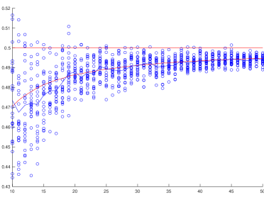
Figure 8: The annealed Heuristic 2a compared to simulation for $p=\log(n)/n$ and $\tau=2/\log(n)$. Horizontal axis: expected average degree. Vertical axis: quasi-stationary infected fraction of the population.

3.2.2 Using graph information: quenched predictions

Heuristic 2a seems to do quite well on average in Figure 8, but there is a lot of variation in the simulation results. The prediction by Heuristic 2a can be computed by just using the parameters $n$, $p$ and $\tau$, so the prediction is annealed and can be made before generating the graph. Can we predict the stationary infected fraction more accurately after generating the graph and using characteristics of the graph? This would be quenched prediction.

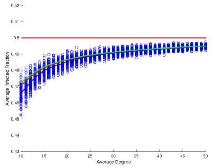
Figure 9: The quenched Heuristics 2b (green) and 3 (red) compared to simulation (blue) for $p=\log(n)/n$ and $\tau=2/\log(n)$. The horizontal axis gives the exact average degree.

To test this, we again generated Erdős-Rényi graphs with the same numbers of nodes as in Figure 8, now 100 realizations for each size $n$. If $p=\log(n)/n$, the expected total number of edges is $p\binom{n}{2}=\tfrac{1}{2}(n-1)\log(n)$. This time we conditioned the graphs to have the number of edges exactly equal to its (rounded) expectation. We can even eliminate the rounding error by slightly adjusting $p$. The simulation results are shown in Figure 9. The horizontal coordinate now is the exact average degree, since we fixed the number of edges to its expectation. This exact average degree is a quenched parameter, which can only be computed after observing the graph.

It turns out that graphs with the same exact average degree have a lot less variation in their quasi-stationary means than graphs merely having the same expected average degree. So a lot of the variation is explained by variation of the number of edges in the graph. The prediction therefore becomes more accurate by the following quenched prediction method: first estimate $p$ based on the observed number of edges, then use this adjusted $p$ for estimating the metastable infected fraction. The resulting heuristic is:

Heuristic 3.

Let $G$ be an Erdős-Rényi graph with $n$ nodes and $m$ edges. Consider the contact process on $G$ with infection rate $\tau$. The quasi-stationary infected fraction $\mu$ satisfies

$$\frac{\mu}{n}=\sum_{d=0}^{n-1}P\left(n,\frac{m}{\binom{n}{2}},d\right)\cdot\frac{d\tau\mu}{n+d\tau\mu}.$$ (16)

Here $P(n,p,d)$ is an approximation to the probability $\mathbb{P}(\text{Bin}(n-1,p)=d)$.

This heuristic is given in Figure 9 by the red curve. It is a function of the exact average degree $m/\binom{n}{2}$. A thing that becomes visible now is that this prediction still seems to have a small systematic bias, especially for the smaller values of $n$. We will discuss systematic errors in Heuristic 2 and 3 in the next section.

Heuristic 3 uses the exact number of edges in the graph, which is equivalent to using the sum of the degrees. Next steps would be to use all individual degrees or even the full adjacency matrix $A$ of the graph. If the full degree sequence is known, we could use Heuristic 2b with the exact numbers $\#\{i:d_{i}=d\}$. It turns out by simulations that this is more accurate than Heuristic 2a, but does not lead to an improvement over Heuristic 3, see again Figure 9. A remark to be made here is that now graphs with the same exact average degree might get different predictions. The curve for Heuristic 2b only shows the average of these predictions. This means that prediction errors for individual graph realizations can not be seen in the picture.

To see individual errors, we simulated the contact process on 100 Erdős-Rényi graphs with $n=400$ nodes, $p=1/\sqrt{n}$ and $\tau=2/\sqrt{n}$. Figure 10 gives boxplots for the errors: the difference between the predicted infected fraction and the simulated infected fraction for the different heuristics. In particular this picture shows that quenched predictions are more accurate. Indeed, the errors for Heuristics 1 and 2a have much more variation. On the other hand, more detailed information than the number of edges does not improve the predictions: Heuristic 3 is not worse than Heuristic 2b and 4. Heuristic 4 (to be discussed next) has a small variation, but a large systematic error. The systematic errors of Heuristics 3 and 2b are relatively small, but the situation gets worse when the graph is more sparse, in particular when the graph disconnects. In general, these heuristics work quite well on graphs which are fairly homogeneous such as the complete graph or Erdős-Rényi graph with enough edges. For less homogeneous graphs like power-law graphs, other heuristics are needed.

Now assume the full adjacency matrix is known. Writing again $f_{i}$ for the fraction of time $i$ is infected, and assuming independence between nodes, we find that $i$ gets infected at rate $\tau\sum_{j:i\sim j}f_{j}$. Therefore $f_{i}$ satisfies

$$f_{i}=\frac{\tau\sum_{j:i\sim j}f_{j}}{1+\tau\sum_{j:i\sim j}f_{j}}.$$ (17)

Solving this system of $n$ equations and $n$ unknowns gives a quenched prediction $\hat{f}_{i}$, after which the infected fraction of the population can be predicted by

Heuristic 4.

Let $G=(V,E)$ be an Erdős-Rényi graph. Consider the contact process on $G$ with infection rate $\tau$. Let $\hat{f}_{i},i\in V$ be the solution of the system (17). The quasi-stationary infected fraction $\mu$ satisfies

$$\frac{\mu}{n}=\frac{1}{n}\sum_{i=1}^{n}\hat{f}_{i}.$$ (18)

One would expect this to be more accurate than Heuristic 2b. However, our simulations show it to be obviously worse. In the next section we explain how this is possible.

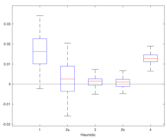
Figure 10: Error boxplots for each heuristic for Erdős-Rényi graphs with $n=400$, $p=1/\sqrt{n}$ and $\lambda=2$. From left to right: Heuristic 1 (comparison to complete graph), Heuristic 2a (using parameters $n,p,\tau$), Heuristic 3 (using exact number of edges), Heuristic 2b (using exact degrees), Heuristic 4 (using full adjacency matrix).

3.3 Systematic errors I: size bias and the infection paradox

Heuristics 2a, 2b and 3 are all based on the assumption that the neighbors of a random node $i$ are infected a fraction $\mu/n$ of time. However, given the information that $j$ is a neighbor of $i$, the degree distribution of $j$ is different. This is the so-called friendship paradox, and the degree distribution of $j$ is called the size-biased distribution [25]. Indeed

$$\mathbb{P}(d_{j}=d\mid i\sim j) =\mathbb{P}(\text{Bin}(n-2,p)=d-1).$$ (19)

For large $n$ and small $p$, this results in

$$\mathbb{P}(d_{j}=d\mid i\sim j)\approx\mathbb{P}(d_{i}=d-1),$$ (20)

so that the expected degree of $j$ is about $np+1$ rather than $np$. So we make an error of 1 in counting the neighbors at distance 1 of $j$. This error causes an underestimation of the fraction of time neighbors of $i$ are infected, which in turn also leads to underestimation for $i$ itself.

The friendship paradox thus implies an infection paradox:

Paradox 1.

An average neighbor of an average node is more often infected than the node itself.

In Figure 11 we see an illustration of this paradox. We simulated an Erdős-Rényi graph with $n=1000$, $p=\log(n)/n$ and $\tau=2/\log(n)$. For each node, we computed the fraction of time it was infected (horizontal axis) and the mean fraction of time its neighbors were infected (vertical axis). On average, nodes are infected 46.1% of time, but neighbors are infected 49.7% of time. Most of the points (606 out of 1000) are above the diagonal, meaning that neighbors of a node are more often infected than the node itself. Observe that also the shape of the distribution is different: taking the average over neighbors gives a more concentrated distribution than directly looking at infection times of nodes.

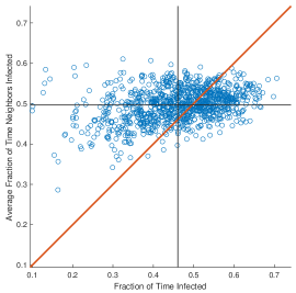
Figure 11: The infection paradox: most nodes are less often infected than their neighbors. Averages are indicated by the horizontal and vertical line, they intersect clearly above the diagonal.

Let again $i$ be a random node and $j$ a random neighbor of $i$. Instead of assuming that $i$ and $j$ themselves have the same degree distribution, now assume that neighbors of $j$ have the same degree distribution as neighbors of $i$. Note that this assumption is still not entirely correct, we now essentially make an error of 1 in counting neighbors at distance 2 of $j$. In a tree-like graph this error is of a smaller order. Under this improved assumption, we obtain

$$\frac{\tilde{\mu}}{n}=\sum_{d=1}^{n-1}\mathbb{P}(\text{Bin}(n-2,p)=d-1))\cdot\frac{d\tau\tilde{\mu}}{n+d\tau\tilde{\mu}}$$ (21)

where $\tilde{\mu}/n$ is the fraction of time a random neighbor of a random node is infected. This motivates to adapt Heuristic 2 and to estimate $\mu/n$ by

$$\frac{\mu}{n}=\sum_{d=0}^{n-1}\mathbb{P}(\text{Bin}(n-1,p)=d))\cdot\frac{d\tau\tilde{\mu}}{n+d\tau\tilde{\mu}}.$$ (22)

The infection paradox leads to underestimation of $\mu/n$, so this adaptation will increase the estimates.

3.4 Systematic errors II: neighbor correlation

Another aspect we ignored so far is dependence between neighboring nodes. Neighbors tend to align into the same state. When a node $i$ is healthy, this increases the likelihood of its neighbors being healthy as well. By ignoring this, we overestimate the rate at which $i$ gets infected by its neighbors.

To illustrate the phenomenon of neighbor correlation, we simulated the process on an Erdős-Rényi graph with $n=1000$ nodes, $p=\log(n)/n$ and $\lambda=2$. For each edge $(i,j)$ in the graph, (co)variances are given by

$$\text{Var}(X_{i}) =\mathbb{E}(X_{i}^{2})-(\mathbb{E}(X_{i}))^{2}=\mathbb{P}(X_{i}=1)-\mathbb{P}(X_{i}=1)^{2},$$ (23)

$$\text{Cov}(X_{i},X_{j}) =\mathbb{E}(X_{i}X_{j})-\mathbb{E}X_{i}\cdot\mathbb{E}X_{j}$$

$$=\mathbb{P}(X_{i}=X_{j}=1)-\mathbb{P}(X_{i}=1)\cdot\mathbb{P}(X_{j}=1).$$ (24)

These are estimated by the corresponding simulated fractions of time, after which we can also estimate the correlation coefficients

$$\rho(X_{i},X_{j})=\frac{\text{Cov}(X_{i},X_{j})}{\sqrt{\text{Var}(X_{i})\text{Var}(X_{j})}}.$$ (25)

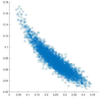
Figure 12: Each marker represents an edge $(i,j)$. The horizontal coordinate is the product of the fractions of time $i$ and $j$ are infected. Vertical is their correlation coefficient.

In Figure 12, we plot the estimated correlation coefficients against the estimated product $\mathbb{P}(X_{i}=1)\cdot\mathbb{P}(X_{j}=1)$. As expected, the correlations are clearly positive. Further note that the correlation is weaker if the nodes are more often infected. This can be explained as follows: a node which is frequently infected has more neighbors, so that the influence of an individual neighbor is less important. In fact, taking on the horizontal axis the product of the degrees instead would give a similar picture.

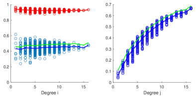
Figure 13: Dependence of conditional probabilities $\mathbb{P}(X_{j}=1\mid X_{i}=0)$ on the degrees $d_{i}$ and $d_{j}$.

All heuristics in the previous section use the assumption that the rate at which node $i$ is infected by node $j$ is equal to $\tau\cdot\mathbb{P}(X_{j}=1)$. However, node $j$ is only able to succesfully infect $i$ if $i$ is healthy. Therefore, the actual rate at which $j$ infects $i$ is equal to

$$\tau\cdot\mathbb{P}(X_{j}=1\mid X_{i}=0),$$ (26)

which is smaller than $\tau\cdot\mathbb{P}(X_{j}=1)$ due to correlations. In Figure 13, we see how the conditional probability $\mathbb{P}(X_{j}=1\mid X_{i}=0)$ depends on the degree of $i$ and the degree of $j$.

The left plot shows for each node $i$ a simulated estimate of

$$\frac{1}{d_{i}}\sum_{j:i\sim j}\mathbb{P}(X_{j}=1\mid X_{i}=0),$$ (27)

the average fraction of time its neighbors are infected, given that $i$ itself is healthy (blue markers). The plot shows that this quantity only mildly depends on the degree of $i$. The variation in this average of conditional probabilities is mainly explained by the variation in the degrees of the neighbors of $i$. Taking for each node $i$ the ratio

$$\frac{\sum_{j:i\sim j}\mathbb{P}(X_{j}=1\mid X_{i}=0)}{\sum_{j:i\sim j}\mathbb{P}(X_{j}=1)},$$ (28)

we get very little variation (red markers). It therefore seems quite reasonable to base heuristics on the assumption that

$$\frac{1}{d_{i}}\sum_{j:i\sim j}\mathbb{P}(X_{j}=1\mid X_{i}=0)\approx\eta\cdot\frac{1}{d_{i}}\sum_{j:i\sim j}\mathbb{P}(X_{j}=1)$$ (29)

for some constant $0<\eta<1$ which does not depend on $i$ and to try to estimate $\eta$. For each degree $d$, we also plotted the average of the conditional (blue) and of the unconditional probabilities (green),

$$\frac{1}{\#\{i:d_{i}=d\}}\sum_{i:d_{i}=d}\frac{1}{d}\sum_{j:i\sim j}\mathbb{P}(X_{j}=1\mid X_{i}=0),$$ (30)

$$\frac{1}{\#\{i:d_{i}=d\}}\sum_{i:d_{i}=d}\frac{1}{d}\sum_{j:i\sim j}\mathbb{P}(X_{j}=1)$$ (31)

and their ratio’s (28) averaged over $i$ (red). From the values on the green curve, we can reproduce an estimate of the size-biased infected fraction $\tilde{\mu}/n$ by taking a weighted average:

$$\frac{\tilde{\mu}}{n}=\frac{1}{n}\sum_{d=1}^{n-1}\sum_{i:d_{i}=d}\frac{1}{d}\sum_{j:i\sim j}\mathbb{P}(X_{j}=1).$$ (32)

Dependence of $\mathbb{P}(X_{j}=1\mid X_{i}=0)$ on the degree of $j$ is visible in the right plot of Figure 13. Each blue marker now corresponds to a single ordered edge $(i,j)$. Dependence of $\mathbb{P}(X_{j}=1)$ on the degree of $j$ has already been observed before, and here we see very similar patterns for the conditional probabilities $\mathbb{P}(X_{j}=1\mid X_{i}=0)$. Averages of conditional and of unconditional probabilities are again given by the blue and green curve respectively.

4 Taking size-bias and neighbor correlations into account

The two types of systematic errors work in opposite directions. Ignoring the size-bias effect means that we underestimate the fraction of time neighbors of a random node $i$ are infected. Then we also underestimate the rate at which $i$ is infected. Eventually, this comes down to underestimation of the infected fraction $\mu/n$ of the population.

On the other hand, neighbors of a healthy node are less likely to be infected. Ignoring this correlation means that we overestimate the rate at which $i$ is infected, which eventually leads to overestimation of the infected fraction of the population.

It seems that these two opposite errors somehow cancel each other in Heuristics 2 and 3, at least for the parameter values in Figure 10. In Heuristic 4, we do not use the binomial degree distribution anymore, but the exact adjacency matrix. This means that Heuristic 4 does not make the size-bias error. However, it still does make the correlation error. This explains why Heuristic 4 in the end gives a much larger systematic prediction error, see Figure 10.

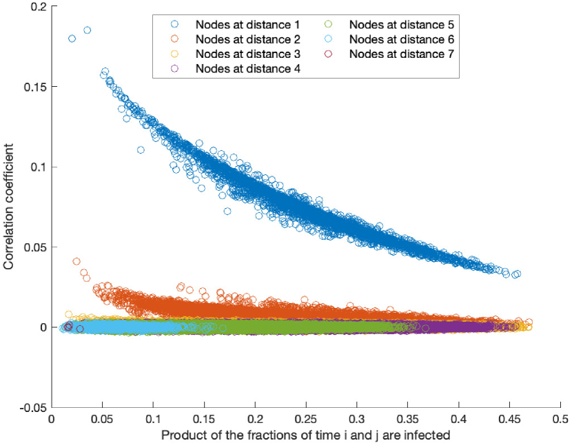
Figure 14: Correlations for each pair of nodes. The color indicates the distance in the graph.

We now will propose heuristics to repair both errors. Presumably, nodes are still positively correlated if they are not direct neighbors. We again simulated the case $n=1000$, $p=\log(n)/n$ and $\lambda=2$. Figure 14 gives for each pair of nodes $i$ and $j$ the estimated correlation coefficient as a function of the product $\mathbb{P}(X_{i}=1)\mathbb{P}(X_{j}=1)$. The color indicates the distance between $i$ and $j$ in the graph. We observe that indeed correlations tend to be positive. Typically, if two nodes have high infection probabilities ($\mathbb{P}(X_{i}=1)\mathbb{P}(X_{j}=1)$ large), then the distance between $i$ and $j$ is small. And finally, correlations rapidly decrease when the distance increases. Based on this last observation, we will design a heuristic which takes correlations between direct neighbors into account, but ignores correlations between other pairs of nodes.

Consider random nodes $i$ and $j$ which are neighbors and have degrees $d_{i}\geq 1$ and $d_{j}\geq 1$. We make the following assumptions:

1. All neighbors of $i$ and $j$ (except $i,j$ themselves) are infected the same fraction of time. We assume this fraction to be independent of $d_{i}$ and $d_{j}$, and equal to the (unknown) size-biased infected fraction $\tilde{\mu}/n$:

   $$\mathbb{P}(X_{k}=1)=\tilde{\mu}/n,\qquad\text{for}\ k\sim i\ \text{or}\ k\sim j,k\neq i,j.$$

2. All these neighbors are assumed to be independent of each other.

3. There exists a constant $\eta\in(0,1)$ such that

   • $\mathbb{P}(X_{k}=1\mid X_{i}=0)=\eta\tilde{\mu}/n$ for each $k\sim i,k\neq j$.

   • $\mathbb{P}(X_{k}=1\mid X_{j}=0)=\eta\tilde{\mu}/n$ for each $k\sim j,k\neq i$.

Note that we do not use degrees other than the degrees of $i$ and $j$. This causes the first assumption to be quite inaccurate for individual nodes, but it does keep the analysis feasible and the errors will mostly average out.

Under these assumptions, we are interested in the simultaneous evolution of nodes $i$ and $j$. This evolution is described by a Markov chain on four states, with transition rates in the diagram in Figure 15.

Figure 15: Transition diagram for infectious status of $i$ and $j$. States are numbered $(1),\ldots,(4)$.

This Markov chain has a unique stationary distribution, which is found by solving the equations

$$\begin{cases}\mathbf{x}^{T}Q=\mathbf{0}^{T},\\ \mathbf{x}^{T}\mathbf{1}=1,\end{cases}\qquad\mathbf{x}^{T}=\begin{pmatrix}x_{1}&x_{2}&x_{3}&x_{4}\end{pmatrix},$$ (33)

where $\mathbf{0}$ and $\mathbf{1}$ are the all zero and all one vector in $\mathbb{R}^{4}$ and $Q=(Q_{k,\ell})$ is the generator matrix:

$$Q=\begin{pmatrix}-\sum_{\ell\neq 1}Q_{1,\ell}&(d_{j}-1)\eta\tilde{\mu}\tau/n&(d_{i}-1)\eta\tilde{\mu}\tau/n&0\\ 1&-\sum_{\ell\neq 2}Q_{2,\ell}&0&((d_{i}-1)\eta\tilde{\mu}\tau/n)+\tau\\ 1&0&-\sum_{\ell\neq 3}Q_{3,\ell}&((d_{j}-1)\eta\tilde{\mu}\tau/n)+\tau\\ 0&1&1&-\sum_{\ell\neq 4}Q_{4,\ell}\end{pmatrix}.$$ (34)

The matrix $Q$ has rank 3 and the equations in (33) have a unique solution, giving $x_{1},\ldots,x_{4}$ as functions of $n$, $\tau$, $d_{i}$, $d_{j}$, $\eta$ and $\tilde{\mu}$. In principle these functions can be determined exactly. We will not do this, but we will show that in this system $X_{i}$ and $X_{j}$ have positive correlation, which vanishes if the degrees go to infinity. This agrees with conjectured and simulated behaviour of the contact process.

First we take a look at the Markov chain for $np\to\infty$. In this case, by the law of large numbers, $(d_{i}-1)/(np)\to 1$ and $(d_{j}-1)/(np)\to 1$ as $n\to\infty$. Since $\tau=\lambda/(np)$ is of order $(np)^{-1}$, all rates to the right are of constant order and asymptotically equal to $\lambda\eta\tilde{\mu}/n$. By symmetry, states (2) and (3) will then have the same stationary probability. The Markov chain therefore asymptotically simplifies to the one in Figure 16. Solving for the stationary distribution of this system, we can easily find $\mathbf{x}$ as well:

$$\mathbf{x}^{T}=\frac{1}{(1+c)^{2}}\cdot\left(1,c,c,c^{2}\right),\qquad\text{where\ }c=\frac{\lambda\eta\tilde{\mu}}{n}.$$ (35)

Figure 16: Transition diagram for infectious status of $i$ and $j$ as $np\to\infty$

We note that from this solution it follows that nodes $i$ and $j$ become independent as the degrees go to $\infty$:

$$\mathbb{P}(X_{i}=0)\cdot\mathbb{P}(X_{j}=0) =(x_{1}+x_{2})(x_{1}+x_{3})=\left(\frac{1+c}{(1+c)^{2}}\right)^{2}=\mathbb{P}(X_{i}=X_{j}=0).$$ (36)

Now consider the more complicated Markov chain of Figure 15. To avoid very awkward calculations, define

$$a=\frac{(d_{i}-1)\eta\tilde{\mu}\tau}{n},\qquad b=\frac{(d_{j}-1)\eta\tilde{\mu}\tau}{n}.$$ (37)

Since $\tau>0$, the rate from $X_{i}=0$ to $X_{i}=1$ is at least $a$. Therefore,

$$\mathbb{P}(X_{i}=0)=x_{1}+x_{2}<\frac{1}{1+a},\qquad\mathbb{P}(X_{j}=0)=x_{1}+x_{3}<\frac{1}{1+b},$$

so that in particular there exist constants $r_{1},r_{2}<1$ for which $x_{1}+x_{2}=r_{1}/(1+a)$ and $x_{1}+x_{3}=r_{2}/(1+b)$. Further, the detailed balance equation for state (1) yields $(a+b)x_{1}=x_{2}+x_{3}$, and hence

$$(2+a+b)x_{1}=2x_{1}+x_{2}+x_{3}=\frac{r_{1}}{1+a}+\frac{r_{2}}{1+b}.$$ (38)

Solving this for $x_{1}=\mathbb{P}(X_{i}=X_{j}=0)$, we obtain

$$\mathbb{P}(X_{i}=X_{j}=0) =\frac{r_{1}(1+b)+r_{2}(1+a)}{(1+a)(1+b)(2+a+b)}$$ (39)

$$>\frac{r_{1}r_{2}}{(1+a)(1+b)}=\mathbb{P}(X_{i}=0)\cdot\mathbb{P}(X_{j}=0),$$ (40)

proving positive correlation for all choices of the parameters.

As noted, given the parameters $n,\tau,d_{i},d_{j}$, we can determine the solution $\mathbf{x}$. However, this solution will still depend on the unknown $\eta$ and $\tilde{\mu}$. To solve for these variables, we need additional equations.

So far, $i$ and $j$ have played the same role. But now we consider $j$ to be a random neighbor of a randomly chosen node $i$. This is only possible if $i$ has degree at least 1. Therefore, $d_{i}$ has distribution $\text{Bin}(n-1,p)$, conditioned on being non-zero. The node $j$ has the size-biased degree distribution $d_{j}-1\sim\text{Bin}(n-2,p)$, which is non-zero by definition. Consequently, $j$ has the same degree distribution as all neighbors of $i$ and $j$ (except $i$ itself). It therefore makes sense to approximate the expected fraction of time $j$ is infected by the same $\tilde{\mu}/n$. Concretely, for each combination of $d_{i}$ and $d_{j}$, we solve the system (33) for $\mathbf{x}$. In particular we get a different solution $\mathbb{P}(X_{j}=1)=x_{2}(d_{i},d_{j})+x_{4}(d_{i},d_{j})$ for each combination $(d_{i},d_{j})$. Then we take a weighted average according to the degree distributions of $i$ and $j$. The resulting equation is

$$\frac{\tilde{\mu}}{n}=\sum_{d_{i}=1}^{n-1}\sum_{d_{j}=1}^{n-1}P^{(\geq 1)}(n,p,d_{i})\tilde{P}(n,p,d_{j})\left(x_{2}(d_{i},d_{j})+x_{4}(d_{i},d_{j})\right),$$ (41)

where $P^{(\geq 1)}(n,p,d_{i})$ and $\tilde{P}(n,p,d_{j})$ are the probabilities that $i$ and $j$ have degrees $d_{i}$ and $d_{j}$ respectively. That is, $P^{(\geq 1)}(n,p,d_{i})=\mathbb{P}(B=d_{i}\mid B\geq 1)$ and $\tilde{P}(n,p,d_{j})=\mathbb{P}(\tilde{B}=d_{j})$ with $B\sim\text{Bin}(n-1,p)$ and $\tilde{B}\sim\text{Bin}(n-2,p)$. Of course these probabilities can be replaced by suitable approximations for large $n$ or by graph-based estimates (see Section 5).

Another equation is obtained by considering conditional probabilities. Since $\mathbb{P}(X_{j}=1\mid X_{i}=0)$ hardly depends on the degree of $i$ (supported by Figure 13), we can assume this conditional probability to be equal to $\eta\tilde{\mu}$. In terms of $\mathbf{x}$, we have $\mathbb{P}(X_{j}=1\mid X_{i}=0)=x_{2}/(x_{1}+x_{2})$. Proceeding along the same lines as above, we obtain

$$\frac{\eta\tilde{\mu}}{n} =\sum_{d_{i}=1}^{n-1}\sum_{d_{j}=1}^{n-1}P^{(\geq 1)}(n,p,d_{i})\tilde{P}(n,p,d_{j})\frac{x_{2}(d_{i},d_{j})}{x_{1}(d_{i},d_{j})+x_{2}(d_{i},d_{j})}.$$ (42)

If all parameters of the process are given, the equations (33), (41) and (42) can be solved to find $\eta$ and $\tilde{\mu}$. Finding exact expressions is a tall order, but an iterative numerical procedure gives satisfactory results.

The solutions for $\eta$ and $\tilde{\mu}$ only depend (in a complicated way) on the process parameters $n$, $p$ and $\tau$. Once they have been determined, we can plug them into $\mathbf{x}$, which will then be a function of the same parameters and the degrees $d_{i}$ and $d_{j}$. This allows to compute an estimate for $\mu$ in the same fashion, by using that $\mathbb{P}(X_{i}=1)=x_{3}+x_{4}$ and taking a weigthed average similar to (41). This time, we first pick a random node $i$. If it has degree 0, it will not contribute to $\mu$ (it quickly heals and never gets infected again). If it has degree $\geq 1$, we let $j$ be a random neighbor of $i$. The estimate for $\mu$ then is

$$\frac{\mu}{n}=\sum_{d_{i}=1}^{n-1}\sum_{d_{j}=1}^{n-1}P(n,p,d_{i})\tilde{P}(n,p,d_{j})\left(x_{3}(d_{i},d_{j})+x_{4}(d_{i},d_{j})\right),$$ (43)

with $P(n,p,d)=\mathbb{P}(\text{Bin}(n-1,p)=d)$. The subtle difference with (41) and (42) is that now $i$ is not conditioned to have degree $\geq 1$, though still degree 0 does not contribute to the sum.

The resulting equations for $\tilde{\mu}$ and $\mu$ can be seen as a more sophisticated version of (21) and (22), which takes size-bias effects and correlations simultaneously into account. We now obtain a new annealed heuristic for predicting $\mu$ as a function of $n$, $p$ and $\tau$:

Heuristic 5.

Let $G=(V,E)$ be an Erdős-Rényi graph with parameters $n$ and $p$. Consider the contact process on $G$ with infection rate $\tau$. For each $1\leq d_{i},d_{j}\leq n-1$, let $\mathbf{x}(d_{i},d_{j})$ be the solution of (33), which depends on the unknowns $\tilde{\mu}$ and $\eta$. Solve (41) and (42) for $\tilde{\mu}$ and $\eta$ and substitute the solutions in $\mathbf{x}(d_{i},d_{j})$. Finally, take the weighted average (43) to obtain a prediction for $\mu$.

Before turning to the numerical results, we wrap up our discussion on asymptotics for $np\to\infty$. The degree distributions of $d_{i}$ and $d_{j}$ concentrate around their expectations, and $\mathbf{x}$ becomes independent of the degrees as in (35). The equations (41) and (42) become

$$\frac{\tilde{\mu}}{n}=x_{2}+x_{4}=\frac{c+c^{2}}{(1+c)^{2}}=\frac{c}{1+c}$$ (44)

$$\frac{\eta\tilde{\mu}}{n}=\frac{x_{2}}{x_{1}+x_{2}}=\frac{c/(1+c)^{2}}{(1+c)/(1+c)^{2}}=\frac{c}{1+c},$$ (45)

and solving them gives

$$\tilde{\mu}=\frac{\lambda-1}{\lambda}n,\qquad\eta=1.$$ (46)

Since $x_{2}=x_{3}$ in this case, we also get $\mu=\tilde{\mu}$. The conclusion is that according to Heuristic 5, both the size-bias effect and the correlations vanish if the degrees go to infinity. This conclusion is consistent with simulations and intuition. Also note that the asymptotic prediction for $\mu$ agrees with Heuristic 1, which can be seen as a small sanity check. Finally, no solution exists for $\lambda<1$, reflecting the fact that the process has no metastable behaviour in this case.

5 Numerical results

5.1 Predicting the infected fraction again

We apply Heuristic 5 to one of our standard test cases: $p=\log(n)/n$ and $\tau=1/(np)$ so that $\lambda=2$. The average degree now only is about $\log(n)$, which is just enough to get an (almost) connected graph. We take graph sizes $n=\lceil e^{k/10}\rceil,k=45,46,\ldots,80$, so that the average degrees vary from 4.5 to 8 in graphs with size ranging from 91 to 2981 nodes. Each size is simulated 100 times. For $P(n,p,d)$, $P^{\geq 1}(n,p,d)$ and $\tilde{P}(n,p,d)$, we take the exact binomial probabilities corresponding to the degree distribution and the size-biased degree distribution respectively. The results are displayed in Figure 17. As before (see Figure 8), the expected average degree is on the horizontal axis, infected fractions on the vertical. Each blue marker corresponds to one graph on which the process is simulated, the blue curve averages over graphs with the same set of parameters, and the red curves are predictions, which are all functions of $n$, $p$ and $\tau$ only. We truncated the picture to zoom in on the curves.

The prediction by Heuristic 5 seems a bit more accurate than previous parameter-based methods, in particular Heuristic 2. Note that the average prediction error is much smaller than fluctuations in the simulations. So the prediction is quite good on average, but it is impossible to reach the same accuracy for individual realisations. Also the graph size plays a role here: the smaller $n$, the more fluctuations in the quasi-stationary infected fraction.

Figure 17: Heuristic 2 (thin red line) and Heuristic 5 (thick red line) compared to simulation (blue) for $p=\log(n)/n$ and $\tau=2/\log(n)$.

Heuristic 5 can be reinforced if information about the graph is available. In particular, we can replace $P(n,p,d)$, $P^{(\geq 1)}(n,p,d)$ and $\tilde{P}(n,p,d)$ with graph-based estimates. We only have to do this for $d\geq 1$. We have the following quenched variants of Heuristic 5:

Heuristic 5 (Variants).

1. Estimate $p$ by the number of edges $m$ in the graph: $\hat{p}=\frac{2m}{n(n-1)}$ and use $P(n,\hat{p},d)$, $P^{(\geq 1)}(n,\hat{p},d)$ and $\tilde{P}(n,\hat{p},d)$.

2. Estimate probabilities by true degree frequencies in the graph:

   $$P(n,p,d)=\frac{\#\{i:d_{i}=d\}}{n}=\frac{1}{n}\sum_{i=1}^{n}\mathbf{1}\{d_{i}=d\},$$ (47)

   $$P^{(\geq 1)}(n,p,d)=\frac{\#\{i:d_{i}=d\}}{\#\{i:d_{i}\geq 1\}}=\frac{\sum_{i=1}^{n}\mathbf{1}\{d_{i}=d\}}{\sum_{i=1}^{n}\mathbf{1}\{d_{i}\geq 1\}},$$ (48)

   $$\tilde{P}(n,p,d)=\frac{1}{\#\{i:d_{i}\geq 1\}}\sum_{i=1,d_{i}\geq 1}^{n}\frac{1}{d_{i}}\sum_{j\sim i}\mathbf{1}\{d_{j}=d\}.$$ (49)

3. Estimate products of probabilities by true frequencies in the graph:

   $$P(n,p,d)\cdot\tilde{P}(n,p,e)=\frac{1}{n}\sum_{i=1}^{n}\sum_{j\sim i}\frac{\mathbf{1}\{d_{i}=d,d_{j}=e\}}{d},$$ (50)

   $$P^{(\geq 1)}(n,p,d)\cdot\tilde{P}(n,p,e)=\frac{1}{\#\{i:d_{i}\geq 1\}}\sum_{i=1}^{n}\sum_{j\sim i}\frac{\mathbf{1}\{d_{i}=d,d_{j}=e\}}{d}.$$ (51)

4. For each combination $d_{i},d_{j}$, solve the system (33). Estimate $\mathbb{P}(X_{j}=1)$ by $x_{2}+x_{4}$ and $\mathbb{P}(X_{j}=1\mid X_{i}=0)$ by $x_{2}/(x_{1}+x_{2})$. Set

   $$\eta_{d_{i},d_{j}}=\frac{\mathbb{P}(X_{j}=1\mid X_{i}=0)}{\mathbb{P}(X_{j}=1)}\approx\frac{x_{2}}{(x_{1}+x_{2})(x_{2}+x_{4})}.$$

   Write $f(i)$ for the fraction of time $i$ is infected (as in Heuristic 4) and solve the system

   $$f(i)=\frac{\tau\sum_{j:j\sim i}\eta_{d_{i},d_{j}}\cdot f(j)}{1+\tau\sum_{j:j\sim i}\eta_{d_{i},d_{j}}\cdot f(j)}.$$ (52)

   to obtain estimates $\hat{f}(i)$. Finally estimate

   $$\frac{\mu}{n}=\frac{1}{n}\sum_{i=1}^{n}\hat{f}(i).$$ (53)

We tested these heuristics for the case $n=1000$, $p=\log(n)/n$ and $\tau=2/(np)$ by generating 100 realizations of the graph. For each realization, we computed the errors made by the different heuristics, i.e. the difference between the predicted and simulated infected fraction. See Figure 18 for a comparison of the results. A few remarks:

• Heuristics 2a and 5 are annealed predictions and only use the parameters $n$, $p$ and $\tau$. In the light of the results in Figure 3, annealed estimates necessarily have errors of about this size.

  These heuristics seem to give comparable results for this set of parameters. Heuristic 2a ignores size-bias and correlations, which will make it inferior to Heuristic 5 for smaller $p$. See Section 5.3.

• Heuristics 5a, 5b and 5c use the average degree, individual degrees and degrees of neighboring pairs respectively. All these quenched variants seem quite accurate. The differences between them are small, so apparently knowing the average degree is already sufficient to get high accuracy.

• Heuristic 4 had a large systematic error, since it does take size-bias into account but not correlation. Heuristic 5d is the improved version of Heuristic 4 and does incorporate correlations. There still seems to be a small systematic error, probably due to higher order effects.

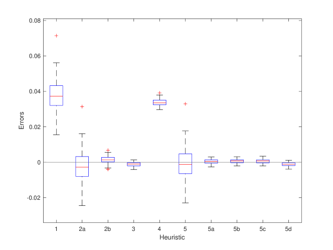
Figure 18: Error boxplots for all heuristics so far for Erdős-Rényi graphs with $n=1000$, $p=\log(n)/n$ and $\lambda=2$.

The effect of correlations and size-bias becomes more important when degrees in the graph are smaller. So far we looked at Erdős-Rényi graphs with $p$ close to or above the connectivity threshold. In these cases, variants of Heuristic 2 still do reasonably well. Below the connectivity threshold, the picture changes. We simulated the contact process on Erdős-Rényi graphs of $1000$ nodes with $p=c/n$ and $c$ ranging from $1.1$ to $7$ $(\approx\log(n))$. In all cases, $\lambda=2$. For each parameter combination and heuristic, an average of $100$ simulations is compared with an average of the corresponding predictions. In Figure 19 we see that variants of Heuristic 5 clearly outperform variants of Heuristic 2. Ignoring correlations and size-bias might lead to serious estimation errors. For really small $p$, Heuristic 5 fails to give good predictions. The reason is that a substantial fraction of the nodes is not in the largest component. For a further discussion in this parameter regime, see Section 5.3.

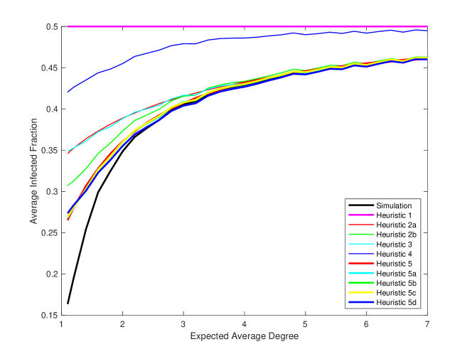
Figure 19: Sparse Erdős-Rényi graphs: average of simulations compared to predictions by all different heuristics.

5.2 Estimating per-node infected fractions, correlations and the total variance

The ideas behind Heuristic 5 give more information than just a prediction for $\mu$. After solving all equations, we know $\mathbf{x}(d_{i},d_{j})$ for all combinations of $d_{i}$ and $d_{j}$. This means that we can make degree-dependent predictions. For instance, to estimate the fraction of time a random node of degree $d$ is infected, take $d_{i}=d$ and average over $d_{j}$ (cf. (43)). Similarly, we can estimate conditional probabilities.

Figure 20: Infection probabilities and conditional infection probabilities for pairs $(i,j)$. Estimates (blue) and predictions (red) for $\mathbb{P}(X_{j}=1\mid X_{i}=0)$ (solid) and $\mathbb{P}(X_{j}=1)$ (dashed). Left: averaged over neighbors of $i$ and as function of $d_{i}$. Right: as function of $d_{j}$.

For illustration, we simulated the process on an Erdős-Rényi graph with $p=\log(n)/n$ and $\lambda=2$. We examined each pair of neighbors $(i,j)$ and estimated $\mathbb{P}(X_{j}=1\mid X_{i}=0)$ by the corresponding simulated fraction of time. For each node $i$ we averaged over its neighbors $j$ and plotted this average as a function of $d_{i}$ in Figure 20, left plot. The solid blue line is the average over all $i$ with given degree. The dashed blue line is the average of ‘unconditional’ probabilities $\mathbb{P}(X_{j}=1)$. We use quotations, since we are still looking at the same nodes, and each of them has a neighbor with degree $d_{i}$. This means that there is still dependence on $d_{i}$, but not on the infectious status of $i$ . Similarly we estimated $\mathbb{P}(X_{j}=1\mid X_{i}=0)$ and $\mathbb{P}(X_{j}=1)$ as a function of $d_{j}$ (right plot). All this is essentially the same as Figure 13, but now we can predict these quantities as follows.

Let $i$ and $j$ be neighboring nodes. First we solve for $\mathbf{x}(d_{i},d_{j})$ as in Heuristic 5. An approximation for $\mathbb{P}(X_{j}=1\mid X_{i}=0)$ is $x_{2}/(x_{1}+x_{2})$. Fixing $d_{i}$ and taking a weighted average over all values of $d_{j}$ gives a prediction for $\mathbb{P}(X_{j}=1\mid X_{i}=0)$ as function of $d_{i}$. Similarly, we get predictions as function of $d_{j}$. These predictions are as in (42), but now only summing over $d_{j}$ or only over $d_{i}$ respectively. These predictions are given by the solid red curves in Figure 20. For the unconditional probabilities $\mathbb{P}(X_{j}=1)$, the procedure is analogous, but now using (41), see the dashed red curves. In fact, by looking at pairs, we are predicting a version of a size-biased distribution here. Similar methods can be used to predict the infected fraction of time for a random node with degree $d_{i}$ using (43) and only summing over $d_{j}$.

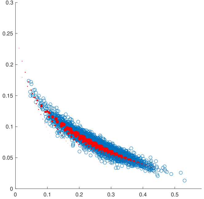
Figure 21: Simulated correlations (blue) and estimated correlations (red).

Another feature of interest are correlations between neighbors. For an edge $(i,j)$ with degrees $d_{i}$ and $d_{j}$, we can again solve for $\mathbf{x}(d_{i},d_{j})$ and then predict the correlation coefficient of $i$ and $j$ by the formula

$$\rho(X_{i},X_{j})\approx\frac{x_{4}-(x_{3}+x_{4})\cdot(x_{2}+x_{4})}{\sqrt{(x_{3}+x_{4})(1-(x_{3}+x_{4}))\cdot(x_{2}+x_{4})(1-(x_{2}+x_{4}))}},$$ (54)

based on (25). Plotting this against

$$\mathbb{P}(X_{i}=1)\cdot\mathbb{P}(X_{j}=1)\approx(x_{3}+x_{4})\cdot(x_{2}+x_{4})$$ (55)

gives Figure 21. The left hand sides of (54) and (55) are simulated, the right hand sides are predictions. For each combination of degrees $d_{i}$ and $d_{j}$, there is one predicted point, plotted as a red marker. The size of the marker is proportional to the probability of the degree pair $(d_{i},d_{j})$. We see that correlations are maybe slightly underestimated for the less likely degree combinations. This could be explained by the fact that Heuristic 5 ignores correlations at distance 2 and larger.

One could wonder if we can use these correlation estimates to obtain predictions for the variance of the number of infected nodes. We have

$$\text{Var}\left(\sum_{i=1}^{n}X_{i}\right)=\sum_{i=1}^{n}\text{Var}(X_{i})+2\sum_{i\neq j}\text{Cov}(X_{i},X_{j}).$$ (56)

For instance, in the complete graph expectation and variances are known: $\mathbb{E}[X_{i}]=1-\frac{1}{\lambda}$, $\text{Var}(X_{i})=\frac{1}{\lambda}(1-\frac{1}{\lambda})$ and $\text{Var}(\sum X_{i})=\frac{n}{\lambda}$. Substituting in (56) gives

$$\frac{n}{\lambda}=\frac{n}{\lambda}(1-\frac{1}{\lambda})+n(n-1)\text{Cov}(X_{1},X_{2}),$$ (57)

So we can compute the covariances as well to find $\text{Cov}(X_{1},X_{2})\sim 1/(n\lambda^{2}).$ This means that pair covariances are small compared to node variances, but the sum of covariances significantly contributes to the total variance.

In the Erdős-Rényi graph, we can estimate $\mu=\sum\mathbb{E}[X_{i}]$ as in (43). Similarly, we estimate the sum of variances $\sum\text{Var}(X_{i})=\sum\mathbb{E}[X_{i}^{2}]-\mathbb{E}[X_{i}]^{2}$ by taking a weighted average of degree-dependent predictions.

For covariances of neighbors, we have degree-dependent predictions $\text{Cov}(d_{i},d_{j})$ as well in the numerator of 54. This can be used to predict

$$2\sum_{i\sim j}\text{Cov}(X_{i},X_{j})\approx pn(n-1)\sum_{d_{i}=1}^{n-1}\sum_{d_{j}=1}^{n-1}\tilde{P}(n,p,d_{i})\tilde{P}(n,p,d_{j})\text{Cov}(d_{i},d_{j}).$$ (58)

The right hand side is twice the expected number of edges, multiplied by the predicted covariance for a randomly chosen edge. A subtlety to be noted here is the weighting: if we pick a random edge, then both endpoints have the size-biased degree distribution.

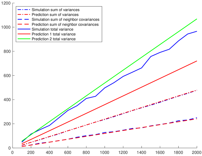
Figure 22: Simulations and predictions of variances and covariances.

What is still missing to predict the total variance in (56) are covariances for pairs of non-neighboring nodes. Figure 22 shows simulations and predictions for the terms

$$\sum_{i}\text{Var}(X_{i}),\qquad 2\sum_{i\sim j}\text{Cov}(X_{i},X_{j}).$$ (59)

Both terms are predicted quite accurately. However, the sum of these two (solid red in the figure) turns out to be a bad prediction for the total variance, which was simulated as well. This means that we can not ignore correlations between nodes at mutual distance 2 or larger. The covariances $\text{Cov}(X_{i},X_{j})$ for $i\not\sim j$ are much smaller, but the number of pairs is much larger, making the sum a significant contribution to the total variance. Since Heuristic 5 is based on analysis of direct neighbors, it falls short to predict the total variance.

There is however another way to predict the total variance. In equilibrium, the total healing rate is equal to $\mu n$. By definition of equilibrium, this is equal to the total infection rate. For a uniformly at random selected set of $\mu n$ nodes, we expect $p\mu(1-\mu)n^{2}$ edges to its complement. The set of infected nodes is not a uniform selection (e.g. high degrees are overrepresented). Still, if the number of infected $k$ is close to equilibrium, we can assume that the number of edges to the complement is proportional $k(n-k)$. In equilibrium ($k=\mu n$), the total infection rate is $\tilde{p}\tau\mu(1-\mu)n^{2}$, where $\tilde{p}$ is a conditional edge probability given that we consider a healthy and an infected node. This gives the equilibrium equation

$$\mu n=\tilde{p}\tau\mu(1-\mu)n^{2},$$ (60)

so that $\tilde{p}\tau$ is equal to the reciprocal of the number $(1-\mu)n$ of healthy nodes in equilibrium. Note that this is consistent with the complete graph, when $p=\tilde{p}=1$.

Now suppose the number of infected deviates a bit from equilibrium and is equal to $k=\mu n+d$. The ratio of total infection and total healing rate is then given by

$$\frac{\tilde{p}\tau(\mu n+d)((1-\mu)n-d)}{\mu n+d}=1-\frac{d}{(1-\mu)n}.$$ (61)

In this formula, we see a drift towards the equilibrium $\mu n$. This type of drift is known to lead to a Gaussian metastable distribution with variance $(1-\mu)n$, see [1]. Since we have an estimate for $\mu$, we have an estimate for the variance as well, which is added to the plot in Figure 22 (solid green). This improves the prediction based on Heuristic 5, but is still biased. A better understanding of correlations of non-neighboring nodes will be needed to get more accurate variance estimates.

5.3 Estimation in sparse graphs, the regime $p=c/n$

The annealed and quenched versions of Heuristic 5 give good results for (almost) connected Erdős-Rényi graphs, i.e. for edge probability $p>\log(n)/n$. For smaller $p$, the graph disconnects and there will be a unique giant component if $p=c/n$ with $c>1$. This giant component has size about $y\cdot n$, with $y$ the largest solution of $1-y=e^{-cy}$, see [25]. All other components will be much smaller, of size at most logarithmic in $n$. The degree distribution inside the giant will differ from the degree distribution in the whole graph. For instance, isolated nodes never appear in the giant. Similarly, size-biased degree distributions inside and outside the giant component are different. In general, degrees inside the giant component will be larger.

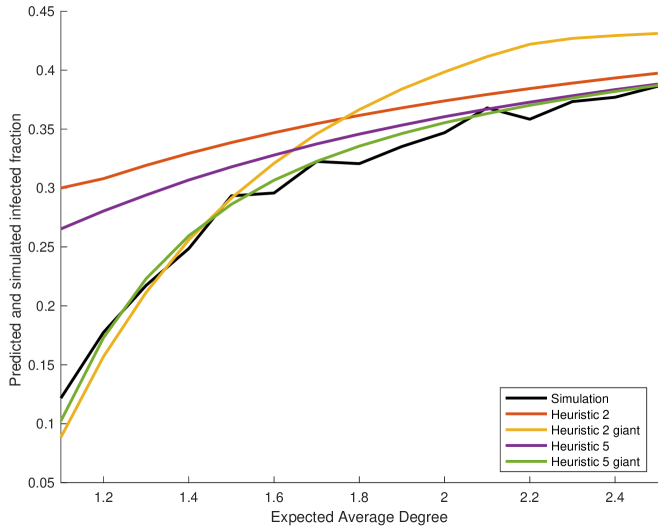
Figure 23: Most heuristics are wrong in very sparse Erdős-Rényi graphs. One should take the degree distribution of the giant and apply size-bias and correlation corrections (green).

Our implementations of Heuristic 5 so far do not account for these properties of subcritical Erdős-Rényi graphs. For the degree distribution they just take the binomials which apply to the whole graph. In Figure 19, we see that all heuristics become less accurate for graphs with really small degrees.

Assuming that the infection quickly disappears outside the giant, we could improve the estimates by analysing the process in the giant and using the corresponding degree distributions. The calculation of these distributions is discussed in Appendix A. Using the results, Heuristic 5 can be used to predict the infected fraction within the giant. After rescaling by the size of the giant, we obtain estimates for $\mu/n$ in the Erdős-Renyi graph.

We followed this procedure for $n=1000$ and $p=c/n$ with $c$ in the range $1.1,1.2,\ldots,2.5$. Figure 23 compares the prediction with the average of a number of realizations of the graph for each value of $c$. The exact number of repetitions depends on $c$, see motivation below. Also added to the plot are a few other predictions, which are all clearly worse:

• Red is Heuristic 2, using the binomial degree distribution, and not correcting for size-bias and correlations.

• Orange is Heuristic 2, using the degree distribution of the giant, but still not correcting for size-bias and correlations.

• Purple is Heuristic 5, using the binomial degree distribution and now correcting for size-bias and correlations. It is better than red.

• Green is Heuristic 5, using the degree distribution of the giant, and correcting for size-bias and correlations.

We conclude that really all things have to be done right to get accurate estimates for the whole range of small $p$. The difference between the different methods becomes much smaller when $c$ increases to $7$ (which is about the connectivity threshold), see Figure 19.

Note that $c$ is the average degree in the graph. The average degree inside a connected component typically is different. In the giant, the average degree is about $c(2-y)>c$ (see Appendix A). All other components are much smaller. Since these components typically are trees, in the largest of them the average degree is close to 2 rather than close to $c$. Taking $1<c<4$ and infection rate $\tau=2/c$, the product of average degree and infection rate will exceed 1 in such components. This means that infection in these components is ‘supercritical’, in the sense that there is a non-trivial equilibrium in which infections and healings are balanced. The only reason that the infection does not survive for a very long time is the size of the component. But it could survive for a moderately long period. Especially when $c$ is close to 1, since this gives the biggest components outside the giant, see Figure 24 for the component structure for $c=1.1$. In this example, the biggest component has size 211, but the second component is quite big as well and has 40 nodes. This means that a simulation of the process on an Erdős-Rényi graph in this regime might need more time to reach the true metastable behaviour. For this reason, Figure 23 was created with less repetitions but longer running times for smaller $c$.

Figure 24: Components in a realization of an Erdős-Rényi graph with $n=1000$ and $p=1.1/n$.

Figure 23 compares predictions with an average over multiple realizations of the graph. This average (the annealed infected fraction) is predicted quite well, but the differences between the quenched infected fractions can be large. In the spirit of variants of Heuristic 5, we could get more accurate estimates after observing the graph. In that case we could for instance use the exact size of the giant, the exact number of edges in the giant, exact frequencies of degrees or exact frequencies of pairs of degrees. Since the predictions on average already are quite good and since similar ideas are discussed in detail before, we do not go deeper into this.

The analysis of the giant serves as a test case for graphs with other degree distributions. Since our methods work quite well in the giant, we expect them to apply to graphs with other degree distributions as well. Which features of the graph are essential to make the methods work requires further research. We expect that the methods are less suitable for graphs with a high variation in degrees (like power-law degree distributions) and for graphs which locally do not look like a tree (like grids). Graphs for which we do expect good results include the random regular graph.

6 Conclusion

We conclude this section by listing a few strengths of Heuristic 5.

1. Heuristic 5 is more accurate than previous heuristics, especially in sparse Erdős-Rényi graphs.

2. We expect that Heuristic 5 can be successfully applied to other (sparse) graphs, like the random regular graph, or to a real-world network given by its adjacency matrix. Further investigation is required to see for which types of graphs Heuristic 5 performs well.

3. Heuristic 5 can be exploited to obtain estimates for other quantities, for instance correlations.

Appendix A Degrees in the giant component

A.1 Degree distribution in the giant component

Here we discuss the degree distribution in the giant component of a sparse Erdős-Rényi graph with edge probability $p=c/n$. Suppose that the graph has been created on $n-1$ nodes and that there is a giant component $C$ of size $y\cdot(n-1)$ for some $0<y<1$. Add the last node to the graph, and connect it to other nodes with probability $p$ independently. To be consistent, the probability that this node does not end up in the giant component has to be close to $1-y$. This gives the equation

$$1-y=(1-p)^{(n-1)y}\sim e^{-cy}.$$ (62)

Indeed it can be shown rigorously that the size $|C|/n$ of the giant is equal to the largest solution to this equation [25], at least asymptotically.

The degree distributions inside and outside the giant can be calculated in the same way. Create all edges between the first $n-1$ nodes, and suppose the giant in this graph has size $C$. Add the final node $v$. The probability that $v$ has degree $k$ and does not end up in the giant is

$$\mathbb{P}(D=k,v\not\in C) =(1-p)^{|C|}\cdot\binom{n-|C|}{k}p^{k}(1-p)^{n-|C|-k-1}.$$ (63)

In this expression $|C|$ is a random variable as well. We can approximate the degree distribution of an arbitrary node by substituting $y\cdot n$ for $|C|$. Further, we assume that $k$ is small compared to $n$, to obtain

$$\mathbb{P}(D=k,v\not\in C) \sim\frac{(c(1-y))^{k}}{k!}e^{-c}.$$ (64)

This gives us

$$\mathbb{P}(D=k,v\in C) =\mathbb{P}(D=k)-\mathbb{P}(D=k,v\not\in C)$$ (65)

$$\sim\frac{(1-(1-y)^{k})c^{k}}{k!}e^{-c},$$ (66)

and leads to the conditional probability

$$\mathbb{P}(D=k\mid v\in C) =\frac{\mathbb{P}(D=k,v\in C)}{\mathbb{P}(v\in C)}$$ (67)

$$\sim\frac{(1-(1-y)^{k})c^{k}}{yk!}e^{-c}.$$ (68)

Now we can as wel find an (asymptotic) estimate for the expected degree in the giant:

$$\mathbb{E}[D\mid v\in C] =\sum_{k=1}^{\infty}\frac{k(1-(1-y)^{k})c^{k}}{yk!}e^{-c}$$

$$=\frac{e^{-c}}{y}\sum_{k=0}^{\infty}\frac{(1-(1-y)^{k+1})c^{k+1}}{k!}$$

$$=\frac{e^{-c}}{y}(ce^{c}-(1-y)ce^{(1-y)c})$$

$$=\frac{c}{y}(1-e^{-2cy})=\frac{c}{y}(1-(1-y)^{2})=c(2-y).$$

If the expected degree $c$ is close to 1, then the expected degree in the giant is close to 2 (the minimum needed for connectedness). If $c$ is large, then $y\approx 1$ and the expected degree inside the giant is approximately the same as the expected degree in the whole graph. This makes sense, since there is (almost) nothing outside the giant.

A.2 Size bias distribution in de giant component

Here we calculate the size-bias degree distribution in the giant component. Let $u$ be an arbitrary node in the giant and let $v$ be a random neighbor of $u$. We are interested in the degree distribution of $v$, which is the size-bias distribution inside the giant.

$$\mathbb{P}(d(v)=k\mid v\leftrightarrow u,u\in C) =\frac{\mathbb{P}(d(v)=k,v\leftrightarrow u,u\in C)}{\mathbb{P}(v\leftrightarrow u,u\in C)}.$$ (69)

Observe that

$$\mathbb{P}(v\leftrightarrow u,u\not\in C) =\mathbb{P}(v\leftrightarrow u)\cdot\mathbb{P}(u\not\in C\mid v\leftrightarrow u)=p\cdot(1-p)^{2|C|}$$ (70)

$$\sim p\cdot e^{-2cy}.$$ (71)

Therefore

$$\mathbb{P}(v\leftrightarrow u,u\in C)=p\left(1-(1-p)^{2|C|}\right)\sim p(1-e^{-2cy}).$$ (72)

Moreover, for $1\leq k\ll n$ we have

$$\mathbb{P}(d(v)=k,v\leftrightarrow u,u\not\in C) =p\cdot(1-p)^{2|C|}\cdot\binom{n-|C|-2}{k-1}p^{k-1}(1-p)^{n-|C|-k-1}$$ (73)

$$\sim\frac{(1-y)^{k-1}n^{k-1}}{(k-1)!}p^{k}e^{-c-cy}$$ (74)

$$=\frac{c^{k}\cdot(1-y)^{k}}{n(k-1)!}e^{-c}.$$ (75)

We further need that

$$\mathbb{P}(d(v) =k,v\leftrightarrow u)=p\cdot\mathbb{P}(\text{Bin}(n-2,p)=k-1)$$ (76)

$$=\binom{n-2}{k-1}p^{k}(1-p)^{n-k-1}$$ (77)

$$\sim\frac{n^{k-1}p^{k}}{(k-1)!}e^{-c}=\frac{c^{k}e^{-c}}{n(k-1)!}.$$ (78)

It now follows that

$$\mathbb{P}(d(v)=k,v\leftrightarrow u,u\in C) =\mathbb{P}(d(v)=k,v\leftrightarrow u)-\mathbb{P}(d(v)=k,v\leftrightarrow u,u\not\in C)$$ (79)

$$=\binom{n-2}{k-1}p^{k}(1-p)^{n-k-1}-\binom{n-|C|-2}{k-1}\cdot p^{k}\cdot(1-p)^{n-k-1+|C|}$$ (80)

$$\sim\frac{c^{k}e^{-c}}{n(k-1)!}\left(1-(1-y)^{k}\right),$$ (81)

which leads to the following size-bias distribution in the giant:

$$\mathbb{P}(d(v)=k\mid v\leftrightarrow u,u\in C) =\frac{p^{k-1}(1-p)^{n-k-1}\left(\binom{n-2}{k-1}-\binom{n-|C|-2}{k-1}\cdot(1-p)^{|C|}\right)}{1-(1-p)^{2|C|}},$$ (82)

The asymptotic approximation is

$$\mathbb{P}(d(v)=k\mid v\leftrightarrow u,u\in C) \sim\frac{p^{k-1}e^{-c}\left(n^{k-1}-((1-y)n)^{k-1}\cdot e^{-cy}\right)}{(k-1)!\cdot(1-e^{-2cy})}$$ (83)

$$=\frac{c^{k-1}e^{-c}\left(1-(1-y)^{k}\right)}{(k-1)!\cdot(1-e^{-2cy})}.$$ (84)

One can check that this sums up to 1.

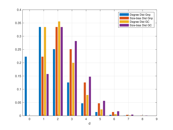
Figure 25: Four different degree distributions for $G_{n,p}$ with $p=\frac{3}{2n}$.

References

- [1] O. S. Awolude, E. Cator, and H. Don. Random walks on with metastable gaussian distribution caused by linear drift with application to the contact process on the complete graph, 2023.
- [2] Shankar Bhamidi, Danny Nam, Oanh Nguyen, and Allan Sly. Survival and extinction of epidemics on random graphs with general degree. Ann. Probab., 49(1):244–286, 2021.
- [3] Béla Bollobás. Random graphs. Academic Press, Inc. [Harcourt Brace Jovanovich, Publishers], London, 1985.
- [4] E. Cator and H. Don. Explicit bounds for critical infection rates and expected extinction times of the contact process on finite random graphs. Bernoulli, 27(3):1556–1582, 2021.
- [5] E. Cator and P. Van Mieghem. Second-order mean-field susceptible-infected-susceptible epidemic threshold. Phys. Rev. E, 85:056111, May 2012.
- [6] E. Cator and P. Van Mieghem. Susceptible-infected-susceptible epidemics on the complete graph and the star graph: Exact analysis. Phys. Rev. E, 87:012811, Jan 2013.
- [7] Odo Diekmann, Hans Heesterbeek, and Tom Britton. Mathematical tools for understanding infectious disease dynamics. Princeton Series in Theoretical and Computational Biology. Princeton University Press, Princeton, NJ, 2013.
- [8] Richard Durrett and Xiu Fang Liu. The contact process on a finite set. Ann. Probab., 16(3):1158–1173, 1988.
- [9] P. Erdős and A. Rényi. On random graphs. I. Publ. Math. Debrecen, 6:290–297, 1959.
- [10] A. Ganesh, L. Massoulie, and D. Towsley. The effect of network topology on the spread of epidemics. In Proceedings IEEE 24th Annual Joint Conference of the IEEE Computer and Communications Societies., volume 2, pages 1455–1466 vol. 2, 2005.
- [11] E. N. Gilbert. Random graphs. Ann. Math. Statist., 30:1141–1144, 1959.
- [12] T. E. Harris. Contact interactions on a lattice. Ann. Probability, 2:969–988, 1974.
- [13] Xiangying Huang and Rick Durrett. The contact process on random graphs and Galton Watson trees. ALEA Lat. Am. J. Probab. Math. Stat., 17(1):159–182, 2020.
- [14] J.O. Kephart and S.R. White. Directed-graph epidemiological models of computer viruses. In Proceedings. 1991 IEEE Computer Society Symposium on Research in Security and Privacy, pages 343–359, 1991.
- [15] Thomas M. Liggett. Multiple transition points for the contact process on the binary tree. Ann. Probab., 24(4):1675–1710, 1996.
- [16] Thomas M. Liggett. Stochastic interacting systems: contact, voter and exclusion processes, volume 324 of Grundlehren der mathematischen Wissenschaften [Fundamental Principles of Mathematical Sciences]. Springer-Verlag, Berlin, 1999.
- [17] T. S. Mountford. A metastable result for the finite multidimensional contact process. Canad. Math. Bull., 36(2):216–226, 1993.
- [18] Thomas Mountford, Daniel Valesin, and Qiang Yao. Metastable densities for the contact process on power law random graphs. Electron. J. Probab., 18:No. 103, 36, 2013.
- [19] Jean-Christophe Mourrat and Daniel Valesin. Phase transition of the contact process on random regular graphs. Electron. J. Probab., 21:Paper No. 31, 17, 2016.
- [20] World Health Organization. From emergency response to long-term COVID-19 disease management: sustaining gains made during the COVID-19 pandemic, volume WHO/WHE/SPP/2023.1. WHO Geneva, 2023.
- [21] Romualdo Pastor-Satorras, Claudio Castellano, Piet Van Mieghem, and Alessandro Vespignani. Epidemic processes in complex networks. Rev. Modern Phys., 87(3):925–979, 2015.
- [22] Romualdo Pastor-Satorras and Alessandro Vespignani. Epidemic dynamics and endemic states in complex networks [j]. Physical review. E, Statistical, nonlinear, and soft matter physics, 63:066117, 07 2001.
- [23] Robin Pemantle. The contact process on trees. Ann. Probab., 20(4):2089–2116, 1992.
- [24] Alan Stacey. The contact process on finite homogeneous trees. Probab. Theory Related Fields, 121(4):551–576, 2001.
- [25] Remco van der Hofstad. Random graphs and complex networks. Vol. 1, volume [43] of Cambridge Series in Statistical and Probabilistic Mathematics. Cambridge University Press, Cambridge, 2017.
- [26] Piet Van Mieghem, Jasmina Omic, and Robert Kooij. Virus spread in networks. IEEE/ACM Transactions on Networking, 17(1):1–14, 2009.
- [27] Yang Wang, D. Chakrabarti, Chenxi Wang, and C. Faloutsos. Epidemic spreading in real networks: an eigenvalue viewpoint. In 22nd International Symposium on Reliable Distributed Systems, 2003. Proceedings., pages 25–34, 2003.