Abstract

Existing neural operator architectures face challenges when solving multiphysics problems with coupled partial differential equations (PDEs), due to complex geometries, interactions between physical variables, and the lack of large amounts of high-resolution training data. To address these issues, we propose Codomain Attention Neural Operator (CoDA-NO), which tokenizes functions along the codomain or channel space, enabling self-supervised learning or pretraining of multiple PDE systems. Specifically, we extend positional encoding, self-attention, and normalization layers to the function space. CoDA-NO can learn representations of different PDE systems with a single model. We evaluate CoDA-NO’s potential as a backbone for learning multiphysics PDEs over multiple systems by considering few-shot learning settings. On complex downstream tasks with limited data, such as fluid flow simulations and fluid-structure interactions, we found CoDA-NO to outperform existing methods on the few-shot learning task by over $36\%$. The code is available at https://github.com/ashiq24/CoDA-NO.

1 Introduction

Figure 1: CoDA-NO, our proposed architecture, generalizes to novel multi-physics systems. CoDA-NO can be pre-trained on fluid dynamics data, a single physics system governed by the Navier-Stocks equation with variables such as velocities ($u_{x},u_{y}$) and pressure $(p)$. The pre-trained CoDA-NO can be easily adapted to a multi-physics fluid-solid interaction system governed by coupled Navier-Stocks and Elastic wave equations. It handles the addition displacement variables ($d_{x},d_{y}$) without any architecture changes.

Many science and engineering problems frequently involve solving complex multiphysics partial differential equations (PDEs) (Strang, ). However, traditional numerical methods usually require the PDEs to be discretized on fine grids to capture important physics accurately. This becomes computationally infeasible in many applications.

Neural operators (Li et al., 2021; Azzizadenesheli et al., 2023) have shown to be a powerful data-driven technique for solving PDEs. Neural operators learn maps between function spaces and converge to a unique operator for any discretization of the functions. This property, called discretization convergence, makes them suitable for approximating solution operators of PDEs. By training on pairs of input and solution functions, we obtain estimates of solution operators that are often orders of magnitude faster to evaluate than traditional PDE solvers while being highly accurate (Schneider et al., 2017; Kossaifi et al., 2023; Bonev et al., 2023).

Neural operators are a data-driven approach and therefore, their performance depends on the quality and abundance of training data. This can be a bottleneck since it is expensive to generate data from traditional solvers or collect them from experiments. A promising approach to dealing with this is to learn physically meaningful representations across multiple systems of PDEs and then transfer them to new problems. Such a self-supervised learning approach with foundation models has found immense success in computer vision and natural language processing (Caron et al., 2021; Radford et al., 2021). Foundation models are trained in a self-supervised manner on large unlabeled datasets. They can be efficiently adapted or fine-tuned to a broad range of downstream tasks with minimal to no additional data or training.

Recent works have delved into the possibility of establishing a foundation model for solving PDEs (Subramanian et al., 2023; McCabe et al., 2023). However, these methods only work on simple, predetermined PDEs with a fixed number of interacting variables. In addition, they are restricted to uniform equidistant grids, which limits their applicability. For example, standard patching-based approaches, used in Vision Transformers (ViTs) (Dosovitskiy et al., 2021), often struggle with discontinuities in predicted functions (Zhang et al., 2022). Further, since they are limited to fixed uniform grids, they cannot be applied to resolutions different from the training resolution.

Our Approach. We propose a novel co-domain transformer neural operator (CoDA-NO) that alleviates the above problems. While previous neural operators have successfully modeled solution operators of one PDE system, our transformer architecture explicitly models dependencies across different physical variables of multiple PDE systems, using self-attention in the co-domain or channel space. Specifically, CoDA-NO tokenizes the functions channel-wise in each layer and treats each physical variable as a token, obviating the need for patching. It also extends the transformer from finite-dimensional vectors to infinite-dimensional functions by appropriately redesigning positional encodings, self-attention mechanism, and normalization.

CoDA-NO can be applied to varying numbers of input functions (on different geometries) and easily adapt to novel PDEs with additional or fewer interacting variables, as illustrated in Fig. 1. This allows us to learn multiple PDE systems in one model. Our proposed framework is highly modular and allows the inclusion of previous neural operators as components. In contrast to the previous works by Li et al. (2023c); Guibas et al. (2021) that extend transformers to operator learning by designing attention on the spatial or temporal domains, in CoDA-NO, we instead design attention on the co-domain or channel space to capture the different physical variables present in multiphysics PDEs and across different PDEs with common physical variables (see Fig. 1).

To assess models’ generalizability across diverse physical systems, we examine two problems. One involves fluid dynamics governed by the Navier-Stokes equation, with velocity and pressure as variables. The other is a fluid-structure interaction problem governed by both the Navier-Stokes equation and the Elastic wave equation, with an additional variable of displacement field associated with the Elastic wave equation. Both of the problems also provide an additional challenge of irregular mesh over a complex geometry.

We pre-train CoDA-NO in a self-supervised manner on snapshots of fluid flows by masking different parts of the velocity or pressure fields. Using few-shot supervised fine-tuning, we show that our model can adapt to unseen viscosities and additional displacement fields given by the elastic wave equation. We use graph neural operator (GNO) layers Li et al. (2023a) as encoders and decoders to handle time-varying irregular meshes of fluid-structure interaction problems. For the few-shot learning problem, our model achieves $36.8\%$ lower errors on average compared to the best-performing baseline trained from scratch on the target problem.

Our contributions are as follows:

• We propose a co-domain attention neural operator that efficiently learns solution operators to PDEs by formulating transformer operations in function space and ensuring discretization convergence.

• The proposed architecture enables self-supervised learning in function space for diverse physical systems by handling varying numbers of input functions and geometries.

• CoDA-NO achieves state-of-the-art performance in generalizing to unknown physical systems with very limited data. That is, CoDA-NO can be viewed as the first foundation neural operator for multiphysics problems.

2 Related Works

Transformers for solving PDEs.

Recently, Takamoto et al. (2023) proposes a method to weight variables/codomains of the input function based on the weights calculated from the PDE parameters. Another study by Li et al. (2023c) proposes a scalable transformer architecture by combining a projection operator to a one-dimensional domain and a learnable factorized kernel. In contrast to these works, CoDA-NO provides a complete attention operator by considering each co-domain as a token function, i.e., infinite dimensional vector, extending traditional transformers on finite dimension tokens.

Self-supervised learning.

Self-supervised learning (SSL) was proposed to tackle the issue of limited labeled data He et al. (2022); Radford et al. (2018); Chen et al. (2020). It allowed the training of large foundation models on massive amounts of data in the field of computer vision and natural language processing. These models are being successfully applied to a wide range of downstream tasks with minimal to no additional task-specific data (Chowdhery et al., 2023; Saharia et al., 2022; Liu et al., 2021; Radford et al., 2021).

Pre-training for PDE solving.

Self-supervised pre-trained models have also been gaining traction in the domain of scientific computing. McCabe et al. (2023) propose pretraining the models with autoregressive tasks on a diverse dataset of multiple PDEs. These models can then be fine-tuned for specific downstream PDEs. Several recent studies have investigated task-agnostic approaches through masking-and-reconstruction (He et al., 2022) and the consistency of representations under symmetry transformations (Xu et al., 2023; Li et al., 2020a; Mialon et al., 2023). Recent work by Subramanian et al. (2023) sheds light on the transferability of these models between different systems of PDEs. While these methods achieve good performance, the target (downstream) PDE must maintain a strict resemblance to the ones used for pretraining. In addition, adapting these models for PDEs with new additional output variables is not possible. ViT-based patching approaches (Zhang et al., 2022) disrupt the continuity and are not resolution-invariant.

3 Preliminaries

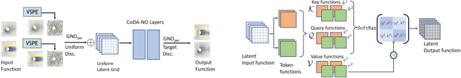
Figure 2: On the left, we illustrate the architecture of the Codomain Attention Neural Operator. Each physical variable (or co-domain) of the input function is concatenated with variable specific positional encoding (VSPE). Each variable, along with the VSPE, is passed through a GNO layer, which maps from the given non-uniform geometry to a latent regular grid. Then, the output on a uniform grid is passed through a series of CoDA-NO layers. Lastly, the output of the stacked CoDA-NO layers is mapped onto the domain of the output geometry for each query point using another GNO layer. On the right, we illustrate the mechanism of codomain attention. At each CoDA-NO layer, the input function is tokenized codomain-wise, and each token function is passed through the ${\mathcal{K}},{\mathcal{Q}},$ and ${\mathcal{V}}$ operators to get key, query, and value functions $\{k^{1},k^{2}\},\{q^{1},q^{2}\},$ and $\{v^{1},v^{2}\}$ respectively. The output function is calculated via an extension of the self-attention mechanism to the function space.

We briefly review the necessary concepts to understand our approach and establish the notation. For any input function $a\colon\mathcal{D}\rightarrow\mathbb{R}^{d_{in}}$, we will denote the $d_{in}$ dimensional output shape as codomain. We consider each of the components of the codomain as different physical variables, which are real-valued functions over the input domain $\mathcal{D}$, i.e., $a=[a^{1},\dots,a^{d_{in}}]$ with $a^{i}:\mathcal{D}\rightarrow\mathbb{R}$. The same applies to the output function $u\colon\mathcal{D}\rightarrow\mathbb{R}^{d_{out}}$.

Neural Operators. Neural operators are a class of deep learning architectures designed to learn maps between infinite-dimensional function spaces (Kovachki et al., 2021). A Neural Operator seeks to approximate an operator $\mathcal{G}$ that maps an input function $a\in\mathcal{A}$ to its corresponding output function $u\in\mathcal{U}$ by building a parametric map $\mathcal{G}_{\phi}:\mathcal{A}\to\mathcal{U}$. The typical architecture of a Neural Operator can be described as

$$\mathcal{G}_{\phi}=\mathcal{P}\circ{\mathcal{I}}_{L}\circ\dots\mathcal{I}_{1}\circ\mathcal{L}.$$ (1)

Here, $\mathcal{L}\colon a\rightarrow w_{0}$ and $\mathcal{P}\colon w_{L}\rightarrow u$ are lifting and pointwise projection operators, respectively. The action of any pointwise operator ${\mathcal{H}}:\{f:\mathcal{D}\rightarrow\mathbb{R}^{d_{f}}\}\rightarrow\{g:\mathcal{D}\rightarrow\mathbb{R}^{d_{g}}\}$ can be defined as

$${\mathcal{H}}[f][x]=h_{\phi}(f(x)),$$ (2)

where $h_{\phi}:\mathbb{R}^{d_{f}}\rightarrow\mathbb{R}^{d_{g}}$ is any function with parameters $\phi$. The integral operator ${\mathcal{I}}_{l}:w_{l-1}\rightarrow w_{l}$ performs a kernel integration over the input function $w_{l-1}$ as

$${\mathcal{I}}_{l}[w_{l-1}](x)=\int_{\mathcal{D}_{l-1}}k_{l}(x,y)w_{l-1}(y)\,\mathrm{d}y.$$ (3)

Here, $\mathcal{D}_{l-1}$ is the domain of the function $w_{l-1}$. In the case of Fourier Neural operators (FNO) (Li et al., 2020a), a convolution kernel, i.e., $k_{l}(x,y)=k_{l}(x-y)$ was used. By the convolution theorem, this enables the representation of an integral operator as a pointwise multiplication of the Fourier coefficients as follows:

$$w_{l}=\mathcal{F}^{-1}(\mathcal{F}(k_{l})\odot\mathcal{F}(w_{l-1})).$$ (4)

In the presence of discretization, the corresponding integration is approximated using a discrete Fourier transform,  i.e., the Riemann sum approximation, and for equidistant grids, can be efficiently computed using a fast Fourier transform (FFT) implementation.

For the Graph neural operator (GNO) (Li et al., 2020b), a small neighborhood $B_{r}(x)\cap\mathcal{D}_{l-1}$ around the point $x$ is considered instead of integrating over the whole domain $\mathcal{D}_{l-1}$, such that Eq. (3) changes to

$$w_{l}(x)=\int_{B_{r}(x)\cap D_{l-1}}k_{l}(x,y)w_{l-1}(y)\,\mathrm{d}y.$$ (5)

Given a set of evaluations of the function $w_{l-1}$ on points $\{y_{i}\}_{i=1}^{n}\subset\mathcal{D}_{l-1}$, the kernel integral can be approximated by

$$w_{l}(x)\approx\sum_{y_{i}\in B_{r}(x)}k_{l}(x,y_{i})w_{l-1}(y_{i})q_{i},$$ (6)

where $q_{i}\in\mathbb{R}$ are suitable quadrature weights (Kovachki et al., 2021). The discretized kernel integral can be viewed as a message passing on graphs, where the neighborhood of each point $x$ consists of all points within radius $r$.

4 Method

Problem Statement. Our goal is to develop a neural operator architecture $\mathcal{G}$ that explicitly models the interaction between physical variables of PDE systems. To learn and predict different systems, the architecture should not be restricted to a fixed number of such variables.

Let’s consider two input functions $a\colon\mathcal{D}\rightarrow\mathbb{R}^{d_{in}}$ and $\tilde{a}\colon\mathcal{D}\rightarrow\mathbb{R}^{\tilde{d}_{in}}$ of two different PDE solution operators with corresponding output functions $u\colon\mathcal{D}\rightarrow\mathbb{R}^{d_{out}}$ and $\tilde{u}\colon\mathcal{D}\rightarrow\mathbb{R}^{\tilde{d}_{out}}$. In general, the functions $a$ and $\tilde{a}$ represent $d_{in}$ and $\tilde{d}_{in}$ physical variables over the domain $\mathcal{D}$ with $d_{in}\neq\tilde{d}_{in}$ . We aim to design neural operator architectures $\mathcal{G}$ that can both be applied to $a$ as well as $\tilde{a}$ despite the different codomains of the input as well as output functions. Such property provides the possibility to evaluate or finetune the operator on PDEs with different numbers of variables than those on which it was trained. In particular, when the PDE systems have overlapping physical variables $\{a^{i}\}_{i=1}^{d_{in}}\cap\{\tilde{a}^{i}\}_{i=1}^{\tilde{d}_{in}}\neq\emptyset$, this naturally allows to transfer learned knowledge from one system to the other. We will next describe the details of the CoDa-NO layers and architecture to achieve this goal.

Permutation Equivariant Neural Operator. As we consider the vector-valued input function $a$ as a set of $d_{in}$ functions $\{a^{1},a^{2},\dots,a^{d_{in}}\}$ that represent different physical variables of the PDE. We seek to construct operators that act on sets of input functions with different cardinalities. For an efficient implementation, we mimic transformer architectures and share weights across different variables. We achieve this by defining permutation equivariant integral operator ${\mathcal{I}}_{per}$ as

$${\mathcal{I}}_{per}[w]=\bigg{[}{\mathcal{I}}[w^{1}_{e}],\dots,{\mathcal{I}}[w^{d_{in}}_{e}]\bigg{]},$$ (7)

where ${\mathcal{I}}$ is a regular integral operator following Eq. (3) and $w^{i}_{e}$ is the codomain group of the input variable $i$. Following the same mechanism, we can also define permutation equivariant pointwise operator ${\mathcal{H}}_{per}$ with a shared pointwise operator ${\mathcal{H}}$ as described in Eq. (2). We will use FNO_per and GNO_per to denote permutation equivariant operators using a shared GNO and FNO, respectively.

CoDA-NO Layer. Given a function $w:\mathcal{D}\rightarrow\mathbb{R}^{d}$, we partition the function into a set of so-called token functions $w^{i}:\mathcal{D}\rightarrow\mathbb{R}^{d^{\prime}}$ for $i\in\{1,\dots L\}$ along the codomain, such that $w=\big{[}w^{1},\dots w^{T}\big{]}$. That is, $w$ represents the codomain-wise concatenation of the token functions $w_{i}$ and $d^{\prime}=\frac{d}{L}$. If no other value is specified, we assume that $d^{\prime}=1$. The CoDA-NO layer now processes the token functions using an extension of the self-attention mechanism to the function space (see Appendix Sec. A.1 and Fig. 2).

Let us begin by introducing a single-head CoDA-NO layer. Later, we will expand the concept to multi-head codomain attention. We extend the key, query, and value matrices of the standard attention (see Appendix Sec. A.1 for details) to operators mapping token functions $w^{i}\colon\mathcal{D}\to\mathbb{R}^{d^{\prime}}$ to key, query, and value functions. We define the key, query, and value operators as

$${\mathcal{K}}:w^{i}\rightarrow\{k^{i}:\mathcal{D}\rightarrow\mathbb{R}^{d_{k}}\},$$ (8)

$${\mathcal{Q}}:w^{i}\rightarrow\{q^{i}:\mathcal{D}\rightarrow\mathbb{R}^{d_{q}}\},$$ (9)

$${\mathcal{V}}:w^{i}\rightarrow\{v^{i}:\mathcal{D}\rightarrow\mathbb{R}^{d_{v}}\}.$$ (10)

Assuming $d_{k}=d_{q}$, we denote by $k^{i}={\mathcal{K}}[w^{i}]$, $q^{i}={\mathcal{Q}}[w^{i}]$, and $v^{i}={\mathcal{V}}[w_{i}]$ the key, query, and value functions of the token functions, respectively.

Next, we calculate the output (token) functions $o^{i}:\mathcal{D}\rightarrow\mathbb{R}^{d_{v}}$ as

$$o^{i}={{\tt Softmax}}\left([\frac{\langle q^{i},k^{1}\rangle}{\tau}\dots\frac{\langle q^{i},k^{T}\rangle}{\tau}]\right)[v^{1},\dots,v^{L}]^{\top}$$ (11)

where $\tau$ is the temperature hyperparameter. Here, $\langle.,.\rangle$ denotes a suitable dot product in the function space. We take the $L^{2}(\mathcal{D},\mathbb{R}^{d_{k}})$-dot product given by

$$\langle q^{i},k^{j}\rangle=\int_{\mathcal{D}}\langle q^{i}(x),k^{j}(x)\rangle\,\mathrm{d}x,$$ (12)

where the integral can be discretized using quadrature rules, similar to the integral operator (see Sec. 3).

To implement multi-head attention, we apply the (single-head) attention mechanism described above separately for multiple heads $h\in\{1,\dots H\}$ using ${\mathcal{K}}^{h},{\mathcal{Q}}^{h},\text{ and }{\mathcal{V}}^{h}$ to obtain $o^{i,h}$. We then concatenate these outputs $o^{i,h}$ along the codomain and get $c^{i}:=[o^{i,1},\dots o^{i,H}]$. Finally, we use an operator

$$\mathcal{M}:\{c^{i}:\mathcal{D}\rightarrow\mathbb{R}^{H\cdot d_{v}}\}\rightarrow\{o^{i}:\mathcal{D}\rightarrow\mathbb{R}^{d_{v}}\}$$ (13)

to get the output function $o^{i}$.

We obtain the output of the attention mechanism by concatenating $o^{i}$ as $o=[o^{1},o^{2},\dots o^{L}]$. Finally, we complete the CoDA-NO layer by applying a permutation equivariant integral operator ${\mathcal{I}}_{per}$ on $o$. When CoDA-NO is acting on functions sampled on a uniform grid, the internal operators $\mathcal{K}^{h},{\mathcal{Q}}^{h},\mathcal{V}^{h},\mathcal{M},$ and ${\mathcal{I}}$ are implemented as FNOs.

Function Space Normalization. Normalization is a vital aspect of deep learning architectures. However, when it comes to neural operators mapping infinite-dimensional functions, this topic remains largely unexplored. We now provide a natural extension. Given a function $w$, let $w^{j}_{e}:\mathcal{D}\rightarrow\mathbb{R}^{d_{l}}$ be the codomain group. Then we calculate the mean $\mu\in\mathbb{R}^{d_{l}}$ and standard deviation $\sigma\in\mathbb{R}^{d_{l}}$ for each codomain group as

$$\mu^{j}=\int_{\mathcal{D}}w^{j}_{e}(x)\,\mathrm{d}x.$$ (14)

$$\sigma^{j}=\bigg{(}\int_{\mathcal{D}}(w^{j}_{e}(x)-\mu^{j})^{\circ 2}\,\mathrm{d}x\bigg{)}^{\circ\frac{1}{2}}.$$ (15)

Here, ${\circ i}$ denotes the elementwise (Hadamard) $i^{th}$-power. The normalization operator can be written as

$${\tt Norm}[w^{j}_{e}](x)=({\mathbf{g}}\oslash\sigma^{j})\odot(w^{j}_{e}(x)-\mu^{j})+{\mathbf{b}},$$ (16)

where ${\mathbf{b}}\in\mathbb{R}^{d_{l}}$ and ${\mathbf{g}}\in\mathbb{R}^{d_{l}}$ are learnable bias and gain vectors and $\oslash$ and $\odot$ denote elementwise division and multiplication operation. This normalization can be seen as an extension of the Instance Normalization(Ulyanov et al., 2016) for function spaces. Similarly, normalziaiton variants, group norm, layer norm, and batch norm extend to operator learning with mentioned defitnion of activation statistics (Ioffe & Szegedy, 2015; Ba et al., 2016; Wu & He, 2018).

Variable Specific Positional Encoding (VSPE). We learn positional encoders $e^{j}:\mathcal{D}\rightarrow\mathbb{R}^{d_{en}}$ for each physical variable $j\in\{1,\dots,d_{in}\}$, for the given vector-valued input function $a=[a^{1},\dots,a^{d_{in}}]$. We concatenate each positional encoding $e^{j}$ with the respective variable $a^{j}:\mathcal{D}\rightarrow\mathbb{R}$ along to codomain to obtain extended input functions $a^{j}_{e}=[a^{j},e^{j}]$. Next, we apply a shared pointwise lifting operator

$$\mathcal{P}:\{a_{e}^{j}:\mathcal{D}\rightarrow\mathbb{R}^{d_{en}+1}\}\rightarrow\{w^{j}_{e}:\mathcal{D}\rightarrow\mathbb{R}^{d}\},$$ (17)

typically with $d>d_{en}+1$. Finally, we concatenate $w^{j}_{e}$, $j\in\{1,\dots d_{in}\}$, to get the lifted function

$$w=[w^{1}_{e},\dots,w^{d_{in}}_{e}]\colon\mathcal{D}\to\mathbb{R}^{d\cdot d_{in}}.$$ (18)

We refer to each $w^{j}_{e}$ as a codomain group.

CoDA-NO Architecture. To effectively handle non-uniform complex geometries, we follow the GINO architecture (Li et al., 2023b) where a GNO is used as an encoding and decoding module. Given a set of evaluations of an input function $a$ on a mesh, as represented by $\{a(x_{i}^{in})\}_{i=1}^{n}$, where $\{x_{i}^{in}\}_{i=1}^{n}\subset\mathcal{D}_{in}$, our first step involves concatenation of each physical variables with respective VSPEs. Next, we use GNO_per to transform the function $a$ into a new function $w_{0}$ on a uniform latent grid, represented by $\{x_{i}^{grid}\}_{i=1}^{n^{\prime}}$. Finally, we apply stacked CoDA-NO layers to $w_{0}$ to obtain the encoded function $w_{l}$, which acts as a representation of the input function $a$.

The decoding module is essentially a mirrored version of the encoding module. It starts by applying another block of stacked CoDA-NO layers to the encoded function $w_{l}$ to obtain $w_{L}$. Subsequently, it uses another GNO_per operator to transform $w_{L}$ on a uniform grid to an approximation $u$ of the solution function on an arbitrary output grid $\{u(x_{i}^{out})\}_{i=1}^{n^{\prime}}$. The architecture is summarized in Fig. 2.

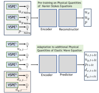
Figure 3: Test time adaptation to new physical variables. The model is pre-trained on the Navier-Stokes equation dataset, which comprises physical variables such as velocities $u_{x}$, $u_{y}$, and pressure $p$. To adapt this pre-trained model on a fluid-solid interaction dataset containing an additional Elastic wave equation with new displacement variables $d_{x}$ and $d_{y}$, it is only necessary to add two additional VSPEs to the whole pipeline.

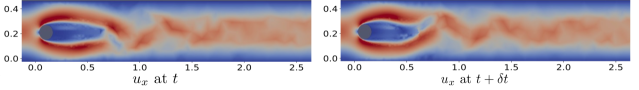
Figure 4: Horizontal velocity $u_{x}$ at $t$ and $t+\delta t$ time step.

Model Training. The model undergoes a two-stage training process: Self-supervised pretraining is followed by a supervised fine-tuning stage. For a summary, we refer to Fig. 3.

Pre-training. In the context of self-supervised pretraining, the objective is to train the model to reconstruct the original input function from its masked version. Within this phase, the model’s encoding component is denoted as the Encoder, while the decoding component comprises the Reconstructor. The values of the input function at a specific percentage of mesh points are randomly masked to zero, and certain variables (of the co-domain) of the input function are entirely masked to zero. The model is then trained to reconstruct the original input from this masked version. We emphasize that the self-supervised learning phase is agnostic of the downstream supervised task and only requires snapshots of simulations of the physical systems.

Fine-tuning. In the supervised fine-tuning phase, the Reconstructor is omitted from the decoding module and replaced by a randomly initialized Predictor module. The parameters of the Encoder and VSPEs are copied from pre-trained weights. If the fine-tuning (target) PDE introduces variables that are not present in the pre-training PDE, we train additional variable encoders for these newly introduced variables (see Fig. 3). This ensures that the model adapts to the expanded set of variables needed for the fine-tuning task.

5 Experiments

Modeling Fluid-structure Interaction. We consider the following problems: (a) a fluid dynamics problem, where a Newtonian, incompressible fluid impinges on a rigid object, and (b) a fluid-structure interaction problem between a Newtonian, incompressible fluid and an elastic, compressible solid object Turek & Hron (2006). We denote $\Omega^{f}_{t}$ (resp. $\Omega^{s}_{t}$) as the domain occupied by the fluid (resp. the solid) at time $t$. The dynamics of the fluid are governed by the Navier-Stokes equations

$$\begin{aligned} &\rho^{f}\frac{\partial u}{\partial t}+\rho^{f}\nabla\cdot(u\otimes u)=\nabla\cdot\bm{\sigma}^{f},~{}\nabla\cdot u=0,\\ \end{aligned}\quad\mbox{in }\Omega^{f}_{t}$$ (19)

where $u$ and $\rho^{f}$ denote the fluid velocity and density, respectively. And $\bm{\sigma}^{f}$ denotes the Cauchy stress tensor, given by

$$\bm{\sigma}^{f}=-p\mathbb{I}+\mu(\nabla u+\nabla u^{T}),$$ (20)

where $\mathbb{I}$ is the identity tensor, $p$ the fluid pressure, and $\mu$ the fluid dynamic viscosity.

For fluid-structure interaction, the deformable solid is governed by the elastodynamics equations

$$\rho^{s}\frac{\partial^{2}d}{\partial t^{2}}=\nabla.(J\bm{\sigma}^{s}(\mathbf{F}^{-1})^{T})\qquad\mbox{ in }\Omega^{s}_{t}$$ (21)

with $\mathbf{F}=\mathbb{I}+\nabla d$ and $J=\det(\mathbf{F})$. Here $d$, $\rho^{s}$, $F$, and $\bm{\sigma}^{s}$ denote the deformation field, the solid density, the deformation gradient tensor, and the Cauchy stress tensor, respectively(see Eq. (28) in the Appendix).

The fluid dynamics (resp. the fluid-structure interaction) problem considers a fluid flow past a fixed, rigid cylinder, with a rigid (resp. elastic) strap attached; details regarding the geometric setup (see Fig. 4), as well as the initial conditions, are provided in the Appendix (see Sec. A.2).

Time-dependent inlet boundary conditions consist of $4^{th}$ order polynomials velocity profiles which vanish at the channel walls (Kachuma & Sobey, 2007; Ghosh, 2017). The inlet conditions are given by

$$u^{\mathcal{I}}_{c_{1},c_{2}}(y,t)=v(t)\cdot\frac{y(y-H)\left(y-c_{1}\frac{H}{2}\right)\left(y-c_{2}\frac{H}{2}\right)}{H(1-c_{1})(1-c_{2})}.$$ (22)

Here $v$ is the ramp function defined as

$$v(t)=\left\{\begin{array}[]{ccl}70\cdot\left(1-\cos\left(\frac{\pi t}{2}\right)\right)&\mbox{if}&0\leq t<2\\ 140&\mbox{if}&t\geq 2\\ \end{array}\right.$$ (23)

and $(c_{1},c_{2})\in\mathcal{I}$, where

$$\mathcal{I}=\left\{(a,b)\in\{-6,-4,-2,0,2,4,6\}^{2}\ |\ a\leq b\right\}$$ (24)

are enforced at the inlet $x=0$. Details regarding the boundary conditions imposed on the strap, which forms the solid-fluid interface, as well as on the remaining domain boundaries, are provided in the Appendix (see Sec. A.2).

Dataset Description and Generation. Two datasets are generated using the TurtleFSI package, one for fluid-structure interaction and the other for fluid dynamics (Bergersen et al., 2020). We simulate the fluid-structure interaction and the fluid dynamics test cases described above up to time $T=10$, using a constant time-step $\delta t=\frac{T}{n}$, where $n=1000$. The data sets are composed of solution trajectories $[u_{t},p_{t},d_{t}]$ (resp. $[u_{t},p_{t}]$), which denote the approximate solution of the fluid-structure interaction problem (resp. the fluid dynamics problem) at times $t=i\delta t,i\in\{0,\dots,n\}$. These trajectories are obtained on the basis of all triplets $(\mu,c_{1},c_{2})$ describing combinations of fluid viscosities and inlet conditions, such that $\mu\in\{1,5,10\},(c_{1},c_{2})\in\mathcal{I}.$ Additional details regarding the solver and simulation parameters used can be found in the Appendix (see Sec. A.2).

Table 1: Test errors ($L_{2}$ loss) for fluid dynamics (NS) and fluid-solid interaction (NS+EW) datasets with viscosity $\mu=5.0$ for different numbers of few-shot training samples.

Model	Pretrain Dataset	# Few Shot Training Samples
		5		25		100
		NS	NS+EW	NS	NS+EW	NS	NS+EW
GINO	-	0.200	0.122	0.047	0.053	0.022	0.043
DeepO	-	0.686	0.482	0.259	0.198	0.107	0.107
GNN	-	0.038	0.045	0.008	0.009	0.008	0.009
Ours	NS	0.025	0.071	0.007	0.008	0.004	0.005
	NS+EW	0.024	0.040	0.006	0.005	0.005	0.003

Experiment Setup. To evaluate the adaptability of the pre-trained model to new PDEs featuring varying numbers of variables, we conduct two distinct pre-training procedures for CoDA-NO and obtain two pre-trained models: ${\tt\mathcal{G}^{p}_{NS-EW}}$ and ${\tt\mathcal{G}^{p}_{NS}}$. The former is pre-trained on a fluid-structure interaction dataset that combines the Navier-Stokes equation and the elastic wave equation, denoted as ${\tt\mathcal{G}^{p}_{NS-EW}}$. The latter, ${\tt\mathcal{G}^{p}_{NS}}$, is pre-trained on a dataset containing fluid motion governed solely by the Navier-Stokes equation. In both scenarios, the pre-training involves utilizing 8000 snapshots of flow and displacement fields, encompassing fluid viscosities $\mu\in\{1,10\}$.

The supervised task involves training the model to predict the state of the system at the subsequent time step based on its current state. For the fluid-structure interaction dataset, we train an operator ${\tt\mathcal{G}_{NS-EW}}$ such that

$${\tt\mathcal{G}_{NS-EW}}:[u_{t},p_{t},d_{t}]\rightarrow[u_{t+\delta t},p_{t+\delta t},d_{t+\delta t}],$$ (25)

where $u,p$, and $d$ are the velocity, pressure, and mesh deformation fields (see Sec. 5). For the data with only fluid motion, we train the operator ${\tt\mathcal{G}_{NS}}$ which maps between the current and next time step velocity and pressure field as

$${\tt\mathcal{G}_{NS}}:[u_{t},p_{t}]\rightarrow[u_{t+\delta t},p_{t+\delta t}].$$ (26)

For both datasets, the pre-trained model is fine-tuned for unseen viscosity $\mu=5.0$ with different numbers of few shot examples. The inlet conditions of these simulations are excluded from the pre-training data. So both viscosity and inlet conditions of the target PDEs are absent in the per-taining dataset. We finetune both of the pre-train models ${\tt\mathcal{G}^{p}_{NS-EW}}$ and ${\tt\mathcal{G}^{p}_{NS}}$ on each dataset.

Baselines. For comparision on the supervised tasks, we train GINO (Li et al., 2023a), DeepONet (Lu et al., 2019), and a graph neural network (GNN) from scratch following Battaglia et al. (2016). To efficiently handle irregular mesh, in the branch network of DeepONet we use a GNN layer followed by MLPs. It should be noted that employing the existing models for pertaining and subsequent finetuning on the target datasets is nontrivial due to complex geometry and the changes in the number of physical variables between the pertaining and target datasets. We report the $L^{2}$ error between the predicted and target functions, which serves as a measure of model performance .

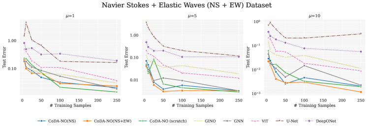
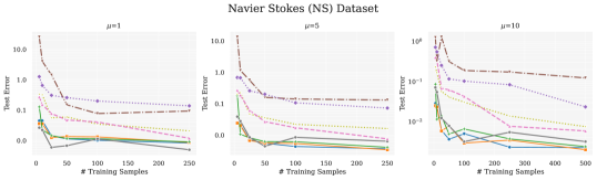
Figure 5: Test Error of different models for different number of training samples.

Implementation Details. The variable encoders are implemented using a multi-layer perceptron mapping the position $x\in\mathcal{D}$ to the embedding vector. Following transformers and NeRF (Mildenhall et al., ) model, we use positional encoding instead of raw coordinates. The Encoder and Reconstructor modules use three stacked CoDA-NO layers. The Predictor modules uses one layer of CoDA-NO.

For masking, 50% of the mesh points of 60% of variables are masked, i.e., set to zero, or 30% of the variables are masked out completely (see Appendix Sec. A.3). For every training sample, one of these two masking choices is selected with equal probability.

Results. In Tab. 1, we report the $L^{2}$ error between the predicted and target functions for each of the methods. We observe that the pre-trained CoDA-NO model performs better than the baselines trained from scratch. Importantly, the performance gain is higher when the number of few-shot examples is very low. This demonstrates the sample efficiency and generalization capability of CoDA-NO to previously unseen physical systems.

Next, when CoDA-NO is pre-trained solely on the Navier-Stokes equation (NS dataset), it shows an impressive ability to adapt to the more challenging fluid-structure interaction PDE (NS+EW dataset). Finally, when CoDA-NO is pre-trained on the more intricate NS+EW dataset, it easily adapts to the simpler NS dataset through fine-tuning.

Table 2: Ablation studies on fluid dynamics (NS) and fluid-solid interaction (NS+EW) datasets with viscosity $\mu=5.0$ for different numbers of few-shot training samples; Reporting $L_{2}$ loss.

Model	Pretrain Dataset	# Few Shot Training Samples
		5		25		100
		NS	NS+EW	NS	NS+EW	NS	NS+EW
ViT	-	0.271	0.211	0.061	0.113	0.017	0.020
U-Net	-	13.33	3.579	0.565	0.842	0.141	0.203
Ours	-	0.182	0.051	0.008	0.084	0.006	0.004
Ours	NS	0.025	0.071	0.007	0.008	0.004	0.005
	NS+EW	0.024	0.040	0.006	0.005	0.005	0.003

Ablation Studies. To evaluate the efficiency of the proposed CoDA-NO layer, VSPE, and codomain-wise tokenization, we compare it against the vision transformer (ViT) (Dosovitskiy et al., 2021) and the Unet (Ronneberger et al., 2015) model.

The mesh points of the NS and NS+EW datasets are irregular and change for each sample. As a result, we cannot directly train ViT and Unet on the dataset. Instead, we follow the architecture of GINO and use a GNN layer to query the latent function on a uniform grid and apply Unet and ViT on the uniform grid, followed by another GNN layer to get the output at the desired query points. We report these comparisons in Tab. 2. On few-shot learning tasks, pre-trained CoDA-NO models outperform the regular transformer base ViT, U-Net models, and CoDA-NO trained from scratch.

We also assess the significance of pre-training, we add a CoDA-NO baseline trained from scratch for each of the datasets. Specifically, we evaluate all the models on all viscosities $\mu\in\{1.0,5.0,10.0\}$ with different numbers of training samples where the initial condition used in these simulations is excluded from the pre-training dataset. The ablation results are shown in Fig. 5.

We observe that when the number of supervised training data is low, the pre-trained CoDA-NO model outperforms other models on most of the dataset. Conversely, with more training samples, the CoDA-NO trained from scratch achieves similar or better performance than the pre-trained model.

Interestingly, when more training data is available, CoDA-NO trained from scratch significantly outperforms all other models, including the regular attention mechanism (ViT), U-Net, and GNN. This illustrates the applicability of the CoDA-NO architecture not just for few-shot learning but also in scenarios where abundant data is available, thanks to its effective attention mechanism for function spaces. We also provide an ablation study where we freeze the parameters of the ”Encoder” and only train the parameters of the ”Predictor”. Here we also perform significantly better than other models on most of the dataset (see Appendix Sec. A.5).

Limitations. In general, CoDA-NO’s performance on target PDEs is influenced by the number of training examples, and we highlight the potential for further enhancement through the integration of physics-informed approaches.

6 Conclusion

In this work, we introduce CoDA-NO, a versatile pre-trained model architecture designed for seamless adaptation to Partial Differential Equations (PDEs) featuring diverse variable compositions. Departing from conventional patch-based attention modules, CoDA-NO innovatively extends the transformer to function spaces by computing attention across co-domains. Leveraging a flexible variable encoding scheme and a graph-based neural operator module, CoDA-NO exhibits adaptability to any target PDE, accommodating new and previously unseen variables with arbitrary input-output geometries during fine-tuning. Our empirical evaluations demonstrate that CoDA-NO consistently outperforms baselines across varying amounts of training data and exhibits robustness in handling missing variables. Our findings on complex multiphysics simulations underscore the efficacy and adaptability of CoDA-NO, positioning it as a valuable tool for addressing challenges in machine learning for PDEs.

Impact Statement

This paper presents work whose goal is to advance the field of Machine Learning and PDEs. Developing open-source foundation models that can be efficiently fine-tuned to solve diverse PDE systems could make high-quality simulations more accessible to academic researchers or other groups with limited resources and accelerate innovation. There might also be potential negative societal consequences of our work, but none of them are immediate to be specifically highlighted here.

Appendix A Appendix

A.1 Attention mechanism for finite-dimensional vectors

Given three sets of vectors, so-called queries $\{{\mathbf{q}}_{i}\}_{i=1}^{N_{q}}$, keys $\{{\mathbf{k}}_{i}\}_{i=1}^{N_{k}}$, and values $\{{\mathbf{v}}_{i}\}_{i=1}^{N_{v}}$ with $N_{k}=N_{v}$ and matching dimensions of queries and keys, attention mechanism calculates weighted sums of the value vectors. Specifically, the set of output vectors $\{{\mathbf{o}}_{i}\}_{i=1}^{N_{q}}$ can be expressed that

$${\mathbf{o}}_{i}={\mathbf{a}}^{i}[{\mathbf{v}}_{1},\dots\mathbf{v}_{N_{v}}]^{\top},\quad i=1,\dots N_{q},$$ (27)

where ${\mathbf{a}}^{i}={\tt SoftMax}[\frac{\langle{\mathbf{q}}_{i},{\mathbf{k}}_{1}\rangle}{\tau},\dots,\frac{\langle{\mathbf{q}}_{i},{\mathbf{k}}_{N_{k}}\rangle}{\tau}]$ and $\tau$ is the temperature term. For the self-attention mechanism, the key, query, and value vectors are calculated from some input sequence $\{{\mathbf{z}}\}_{i=1}^{L}$ using the key, query, and value matrices ${\mathbf{K}},{\mathbf{Q}},$ and ${\mathbf{V}}$ as

$${\mathbf{q}}_{i}={\mathbf{Q}}{\mathbf{z}}_{i},\quad{\mathbf{k}}_{i}={\mathbf{K}}{\mathbf{z}}_{i},\quad{\mathbf{v}}_{i}={\mathbf{V}}{\mathbf{z}}_{i}.$$

A.2 Dataset Description

Fluid structure interaction model.

Under the Kirchoff St-Venant model, the Cauchy stress tensor $\bm{\sigma}^{s}$ verifies

$$\bm{\sigma}^{s}=\frac{1}{J}\mathbf{F}(\lambda^{s}(tr(\mathbf{E}))\mathbb{I}+2\mu^{s}\mathbf{E})\mathbf{F}^{T}$$ (28)

where $\lambda^{s}$ and $\mu^{s}$ are the Lame coefficients, and

$$\mathbf{E}=\frac{1}{2}(\mathbf{F}\mathbf{F}^{T}-\mathbb{I}).$$

Fluid structure interaction geometric setup, boundary and initial conditions.

In the considered setup (see also Figure 4), a fluid flows past a fixed cylinder of radius $R=0.05$ centered at $(x_{c},y_{c})=(0.2,0.2)$ in a two-dimensional channel of length $L=2.5$ and width $H=0.41$. A deformable elastic strap of length $\ell=0.35$ and height $h=0.02$ is attached to the back of the cylinder. Note that, in the test cases considering fluid motion exclusively, the elastic strap is assumed to be rigid.

In the case of the fluid-structure interaction, the interaction conditions arise from the mechanical equilibrium at the boundaries of the strap, which are given by

$$\bm{\sigma}^{f}\cdot\mathbf{n}=\bm{\sigma}^{s}\cdot\mathbf{n}$$

$$u=\frac{\partial d}{\partial t}$$

where $\mathbf{n}$ denotes a unit normal vector to the fluid-solid interface. No-slip boundary conditions are imposed on the fluid velocity at the top (resp .bottom) boundaries of the channel at $y=0$ (resp. $y=H$), as well as on the boundaries of the cylinder and the elastic strap. Outflow boundary conditions are imposed at $x=2.5$ by enforcing the values $p=0$ for the pressure.

The initial conditions

$$(u,p,d)=(0,0,0)$$

where the displacement $d=0$ corresponds to a perfectly horizontal elastic strap and is imposed at time $t=0$.

Details regarding the data set generation.

The TurtleFSI package provides a monolithic solver for the fluid-structure interaction test case, that is, combining the equations describing the solid and fluid evolution into one coupled system based on an Arbitrary Eulerian-Lagrangian (ALE) formulation of the problem and developed on the FEniCS computing environment Logg et al. (2012).

The initial conditions are expressed at set $X=X_{\mathcal{S}}\cup X_{\mathcal{F}}$ of mesh points, corresponding to the union of the solid and fluid domains. In the ALE formulation, at each snapshot $0\leq t\leq t_{M}$ of the simulation, the solution is given at a set of mesh points $X_{t}=X+d_{t}$, where $d_{t}$ denotes the mesh displacement. In particular, the snapshots $u_{t}$ (resp. $p_{t}$) correspond to numerical approximations of the velocity (resp. the pressure) at the mesh points $X_{t}$. Notably, while equation (21) governs the deformation field in the solid domain $\Omega^{s}_{t}$, the displacements $d_{t}$ are obtained through an extension of the deformation field to the fluid domain $\Omega^{f}_{t}$ via a biharmonic extrapolation.

In all the cases considered, the values $\rho^{f}=1.0\times 10^{3}$, $\rho^{s}=1.0\times 10^{3}$, $\lambda^{s}=4.0\times 10^{6}$ and $\mu^{s}=2.0\times 10^{6}$ were used. The simulations were performed using a constant time step $\delta t=0.01$.

A.3 Additional Implementation Details

Masking on Irregular Mesh.

In order to apply masking on an irregular mesh, we select a point at random from the mesh. Following this, we identify the neighboring points within a fixed distance from the selected point and set their values to zero. This process is continued until we have masked out a predetermined portion of all mesh points.

A.4 Super Resolution Test

Here we present the results of our zero-shot super-resolution models, which focused on fluid-solid interaction problems. Specifically, we trained the model using a domain mesh of 1317 points with a given viscosity. During inference, the solution function is queried directly on a denser and non-uniform target mesh consisting of 2193 points.

Table 3: Zero Shot Super Resolution Performance on Fluid-Solid (NS-EW) Interaction Problem

Model	Pretrain Dataset	Fluid Viscocities
		$\mu=5$	$\mu=1$	$\mu=10$
U-Net	-	0.144	0.267	0.216
Vit	-	0.052	0.175	0.046
GINO	-	0.069	0.103	0.0711
GNN	-	0.223	0.211	0.247
CoDA-NO	NS-ES	0.041	0.063	0.048
CoDA-NO	NS	0.032	0.049	0.035

A.5 Additional Experiments

Here, we present some additional ablation studies on our model’s performance when we keeping the weight of the ”Encoder” frozen during supervised fine-tuning.

Table 4: Test errors ($L_{2}$ loss) for fluid dynamics (NS) and fluid-solid interaction (NS+EW) datasets with viscosity $\mu=1.0$ for different numbers of few-shot training samples. The pre-training is done with 8000 samples taken from NS and NS+EW datasets with viscosities $\mu\in\{1.0,10.0\}$.

Model	Pretrain Dataset	# Few Shot Training Samples
		5		10		50		100		250
		NS	NS+EW	NS	NS+EW	NS	NS+EW	NS	NS+EW	NS	NS+EW
Ours	NS	0.0493	0.2645	0.0237	0.1955	0.0092	0.0378	0.0103	0.0604	0.0085	0.0294
	NS+EW	0.0416	0.2371	0.0221	0.1786	0.0105	0.0484	0.0110	0.0380	0.0089	0.0273
CoDA-NO	-	0.1279	0.2435	0.0225	0.2282	0.0117	0.0745	0.0115	0.0219	0.0091	0.0148
GINO	-	0.3337	0.2615	0.3189	0.1817	0.0596	0.0667	0.0349	0.0636	0.0209	0.0308
GNN	-	0.0265	0.1800	0.0222	0.1799	0.0068	0.0867	0.0113	0.0539	0.0050	0.0193
ViT	-	0.2738	0.5087	0.1519	0.4146	0.0473	0.1119	0.0407	0.1106	0.0119	0.0381
U-Net	-	25.33	1.434	4.007	4.320	0.1495	0.6653	0.07723	0.1821	0.0934	0.1651
DeepONet	-	1.262	0.8186	0.6485	0.4937	0.2576	0.3198	0.1992	0.3399	0.1385	0.1916

Table 5: Test errors ($L_{2}$ loss) for fluid dynamics (NS) and fluid-solid interaction (NS+EW) datasets with viscosity $\mu=5.0$ for different numbers of few-shot training samples. The pre-training is done with 8000 samples taken from NS and NS+EW datasets with viscosities $\mu\in\{1.0,10.0\}$.

Model	Pretrain Dataset	# Few Shot Training Samples
		5		10		50		100		250
		NS	NS+EW	NS	NS+EW	NS	NS+EW	NS	NS+EW	NS	NS+EW
Ours	NS	0.0190	0.1597	0.0141	0.0220	0.0043	0.0042	0.0054	0.0053	0.0033	0.0025
	NS+EW	0.0201	0.1077	0.0157	0.0153	0.0053	0.0053	0.0044	0.0030	0.0037	0.0022
CoDA-NO	-	0.1820	0.0513	0.0107	0.0199	0.0063	0.0066	0.0062	0.0045	0.0041	0.0029
GINO	-	0.2004	0.1222	0.2245	0.0753	0.0359	0.0364	0.0222	0.0438	0.0163	0.0190
GNN	-	0.0390	0.0460	0.0280	0.0294	0.0045	0.0123	0.0086	0.0094	0.0064	0.0033
ViT	-	0.2719	0.2113	0.1889	0.1561	0.0271	0.0474	0.0173	0.0207	0.0077	0.0122
U-Net	-	13.3370	3.5790	1.1540	2.1340	0.1608	0.3178	0.1418	0.2035	0.1317	0.1180
DeepONet	-	0.6863	0.4821	0.6720	0.2945	0.2019	0.2024	0.1076	0.1070	0.0731	0.1085

Table 6: Test errors ($L_{2}$ loss) for fluid dynamics (NS) and fluid-solid interaction (NS+EW) datasets with viscosity $\mu=10.0$ for different numbers of few-shot training samples. The pre-training is done with 8000 samples taken from NS and NS+EW datasets with viscosities $\mu\in\{1.0,10.0\}$.

Model	Pretrain Dataset	# Few Shot Training Samples
		5		10		50		100		250
		NS	NS+EW	NS	NS+EW	NS	NS+EW	NS	NS+EW	NS	NS+EW
Ours	NS	0.0186	0.1203	0.0105	0.0207	0.00327	0.00444	0.00391	0.00412	0.00229	0.00215
	NS+EW	0.0171	0.0925	0.0109	0.0130	0.00383	0.00360	0.00303	0.00232	0.00225	0.00133
CoDA-NO	-	0.0859	0.0618	0.0115	0.0166	0.00494	0.00763	0.00660	0.00330	0.00374	0.00195
GINO	-	0.2316	0.1560	0.1679	0.0582	0.04122	0.03327	0.03074	0.0395	0.01389	0.01139
GNN	-	0.0715	0.0448	0.0547	0.0179	0.00789	0.00494	0.00319	0.0148	0.00547	0.00229
ViT	-	0.4001	0.2201	0.3388	0.1967	0.06215	0.05700	0.04299	0.01867	0.00770	0.00903
U-Net	-	1.2550	0.6995	0.3255	0.9148	0.3156	0.2095	0.1889	0.2085	0.1732	0.3132
DeepONet	-	0.7158	0.3794	0.5515	0.2533	0.1164	0.1337	0.1027	0.07814	0.08359	0.05697

References

- Azzizadenesheli et al. (2023) Azzizadenesheli, K., Kovachki, N., Li, Z., Liu-Schiaffini, M., Kossaifi, J., and Anandkumar, A. Neural operators for accelerating scientific simulations and design. arXiv preprint arXiv:2309.15325, 2023.
- Ba et al. (2016) Ba, J. L., Kiros, J. R., and Hinton, G. E. Layer normalization. arXiv preprint arXiv:1607.06450, 2016.
- Battaglia et al. (2016) Battaglia, P., Pascanu, R., Lai, M., Jimenez Rezende, D., et al. Interaction networks for learning about objects, relations and physics. Advances in neural information processing systems, 2016.
- Bergersen et al. (2020) Bergersen, A. W., Slyngstad, A., Gjertsen, S., Souche, A., and Valen-Sendstad, K. turtlefsi: A robust and monolithic fenics-based fluid-structure interaction solver. Journal of Open Source Software, 2020.
- Bonev et al. (2023) Bonev, B., Kurth, T., Hundt, C., Pathak, J., Baust, M., Kashinath, K., and Anandkumar, A. Spherical fourier neural operators: Learning stable dynamics on the sphere. In Proceedings of the International Conference on Machine Learning (ICML), 2023.
- Caron et al. (2021) Caron, M., Touvron, H., Misra, I., Jégou, H., Mairal, J., Bojanowski, P., and Joulin, A. Emerging properties in self-supervised vision transformers. In Proceedings of the IEEE/CVF international conference on computer vision, 2021.
- Chen et al. (2020) Chen, T., Kornblith, S., Norouzi, M., and Hinton, G. A simple framework for contrastive learning of visual representations. In International conference on machine learning. PMLR, 2020.
- Chowdhery et al. (2023) Chowdhery, A., Narang, S., Devlin, J., Bosma, M., Mishra, G., Roberts, A., Barham, P., Chung, H. W., Sutton, C., Gehrmann, S., et al. Palm: Scaling language modeling with pathways. Journal of Machine Learning Research, 2023.
- Dosovitskiy et al. (2021) Dosovitskiy, A., Beyer, L., Kolesnikov, A., Weissenborn, D., Zhai, X., Unterthiner, T., Dehghani, M., Minderer, M., Heigold, G., Gelly, S., et al. An image is worth 16x16 words: Transformers for image recognition at scale. In International Conference on Learning Representations, 2021.
- Ghosh (2017) Ghosh, S. Relative effects of asymmetry and wall slip on the stability of plane channel flow. Fluids, 2017.
- Guibas et al. (2021) Guibas, J., Mardani, M., Li, Z., Tao, A., Anandkumar, A., and Catanzaro, B. Adaptive Fourier neural operators: Efficient token mixers for transformers. arXiv preprint arXiv:2111.13587, 2021.
- He et al. (2022) He, K., Chen, X., Xie, S., Li, Y., Dollár, P., and Girshick, R. Masked autoencoders are scalable vision learners. In Proceedings of the IEEE/CVF conference on computer vision and pattern recognition, 2022.
- Ioffe & Szegedy (2015) Ioffe, S. and Szegedy, C. Batch normalization: Accelerating deep network training by reducing internal covariate shift. In International conference on machine learning. PMLR, 2015.
- Kachuma & Sobey (2007) Kachuma, D. and Sobey, I. Linear instability of asymmetric poiseuille flows. 2007.
- Kossaifi et al. (2023) Kossaifi, J., Kovachki, N. B., Azizzadenesheli, K., and Anandkumar, A. Multi-grid tensorized fourier neural operator for high resolution PDEs, 2023. URL https://openreview.net/forum?id=po-oqRst4Xm.
- Kovachki et al. (2021) Kovachki, N., Li, Z., Liu, B., Azizzadenesheli, K., Bhattacharya, K., Stuart, A., and Anandkumar, A. Neural operator: Learning maps between function spaces. arXiv preprint arXiv:2108.08481, 2021.
- Li et al. (2020a) Li, Z., Kovachki, N., Azizzadenesheli, K., Liu, B., Bhattacharya, K., Stuart, A., and Anandkumar, A. Fourier neural operator for parametric partial differential equations. arXiv preprint arXiv:2010.08895, 2020a.
- Li et al. (2020b) Li, Z., Kovachki, N., Azizzadenesheli, K., Liu, B., Bhattacharya, K., Stuart, A., and Anandkumar, A. Neural operator: Graph kernel network for partial differential equations. arXiv preprint arXiv:2003.03485, 2020b.
- Li et al. (2021) Li, Z., Kovachki, N. B., Azizzadenesheli, K., Bhattacharya, K., Stuart, A., Anandkumar, A., et al. Fourier neural operator for parametric partial differential equations. In Proceedings of the International Conference on Learning Representations (ICLR), 2021.
- Li et al. (2023a) Li, Z., Kovachki, N. B., Choy, C., Li, B., Kossaifi, J., Otta, S. P., Nabian, M. A., Stadler, M., Hundt, C., Azizzadenesheli, K., and Anandkumar, A. Geometry-informed neural operator for large-scale 3d pdes. arXiv preprint arXiv:2309.00583, 2023a.
- Li et al. (2023b) Li, Z., Kovachki, N. B., Choy, C., Li, B., Kossaifi, J., Otta, S. P., Nabian, M. A., Stadler, M., Hundt, C., Azizzadenesheli, K., et al. Geometry-informed neural operator for large-scale 3d pdes. arXiv preprint arXiv:2309.00583, 2023b.
- Li et al. (2023c) Li, Z., Shu, D., and Farimani, A. B. Scalable transformer for pde surrogate modeling. arXiv preprint arXiv:2305.17560, 2023c.
- Liu et al. (2021) Liu, Z., Lin, Y., Cao, Y., Hu, H., Wei, Y., Zhang, Z., Lin, S., and Guo, B. Swin transformer: Hierarchical vision transformer using shifted windows. In Proceedings of the IEEE/CVF international conference on computer vision, 2021.
- Logg et al. (2012) Logg, A., Mardal, K.-A., and Wells, G. Automated solution of differential equations by the finite element method: The FEniCS book. Springer Science & Business Media, 2012.
- Lu et al. (2019) Lu, L., Jin, P., and Karniadakis, G. E. Deeponet: Learning nonlinear operators for identifying differential equations based on the universal approximation theorem of operators. arXiv preprint arXiv:1910.03193, 2019.
- McCabe et al. (2023) McCabe, M., Blancard, B. R.-S., Parker, L. H., Ohana, R., Cranmer, M., Bietti, A., Eickenberg, M., Golkar, S., Krawezik, G., Lanusse, F., et al. Multiple physics pretraining for physical surrogate models. arXiv preprint arXiv:2310.02994, 2023.
- Mialon et al. (2023) Mialon, G., Garrido, Q., Lawrence, H., Rehman, D., LeCun, Y., and Kiani, B. Self-supervised learning with lie symmetries for partial differential equations. In ICLR 2023 Workshop on Physics for Machine Learning, 2023.
- (28) Mildenhall, B., Srinivasan, P. P., Tancik, M., Barron, J. T., Ramamoorthi, R., and Ng, R. Nerf: Representing scenes as neural radiance fields for view synthesis. Communications of the ACM.
- Radford et al. (2018) Radford, A., Narasimhan, K., Salimans, T., Sutskever, I., et al. Improving language understanding by generative pre-training. 2018.
- Radford et al. (2021) Radford, A., Kim, J. W., Hallacy, C., Ramesh, A., Goh, G., Agarwal, S., Sastry, G., Askell, A., Mishkin, P., Clark, J., et al. Learning transferable visual models from natural language supervision. In International conference on machine learning. PMLR, 2021.
- Ronneberger et al. (2015) Ronneberger, O., Fischer, P., and Brox, T. U-net: Convolutional networks for biomedical image segmentation. In Medical Image Computing and Computer-Assisted Intervention. Springer, 2015.
- Saharia et al. (2022) Saharia, C., Chan, W., Saxena, S., Li, L., Whang, J., Denton, E. L., Ghasemipour, K., Gontijo Lopes, R., Karagol Ayan, B., Salimans, T., et al. Photorealistic text-to-image diffusion models with deep language understanding. Advances in Neural Information Processing Systems, 2022.
- Schneider et al. (2017) Schneider, T., Teixeira, J., Bretherton, C. S., Brient, F., Pressel, K. G., Schär, C., and Siebesma, A. P. Climate goals and computing the future of clouds. 2017.
- (34) Strang, G. Computational science and engineering. Optimization.
- Subramanian et al. (2023) Subramanian, S., Harrington, P., Keutzer, K., Bhimji, W., Morozov, D., Mahoney, M., and Gholami, A. Towards foundation models for scientific machine learning: Characterizing scaling and transfer behavior. arXiv preprint arXiv:2306.00258, 2023.
- Takamoto et al. (2023) Takamoto, M., Alesiani, F., and Niepert, M. Learning neural pde solvers with parameter-guided channel attention. arXiv preprint arXiv:2304.14118, 2023.
- Turek & Hron (2006) Turek, S. and Hron, J. Proposal for numerical benchmarking of fluid-structure interaction between an elastic object and laminar incompressible flow. Springer, 2006.
- Ulyanov et al. (2016) Ulyanov, D., Vedaldi, A., and Lempitsky, V. Instance normalization: The missing ingredient for fast stylization. arXiv preprint arXiv:1607.08022, 2016.
- Wu & He (2018) Wu, Y. and He, K. Group normalization. In Proceedings of the European conference on computer vision (ECCV), 2018.
- Xu et al. (2023) Xu, B., Zhou, Y., and Bian, X. Self-supervised learning based on transformer for flow reconstruction and prediction. arXiv preprint arXiv:2311.15232, 2023.
- Zhang et al. (2022) Zhang, B., Gu, S., Zhang, B., Bao, J., Chen, D., Wen, F., Wang, Y., and Guo, B. Styleswin: Transformer-based gan for high-resolution image generation. In Proceedings of the IEEE/CVF conference on computer vision and pattern recognition, 2022.