A program for 3D nuclear static and time-dependent density-functional theory with full Skyrme energy density functional: hit3d

Abstract

This work presents a computer program that performs symmetry-unrestricted 3D nuclear time-dependent density function theory (DFT) calculations. The program features the augmented Lagrangian constraint in the static calculation. This allows for the calculation of the potential energy surface. In addition, the code includes the full energy density functionals derived from the Skyrme interaction, meaning that the time-even and time-odd tensor parts are included for the time-dependent calculations. The results of the hit3d code are carefully compared with the Sky3D and Ev8 programs. The testing cases include unconstrained DFT calculations for doubly magic nuclei, the constrained DFT + BCS calculations for medium-heavy nucleus ¹¹⁰Mo, and the dynamic applications for harmonic vibration and nuclear reactions.

PROGRAM SUMMARY

Program Title: hit3d
CPC Library link to program files:
Code Ocean capsule:
Licensing provisions: CC0 1.0
Programming language: C/C++
Supplementary material:
Nature of problem: The program performs symmetry-unrestricted time-dependent (TD) density-functional theory (DFT) calculations for finite nuclei. For the static calculations, it performs precise constraint calculations using the augmented Lagrangian method. For vibrational calculations, the program performs Fourier analysis of the multipole moments as functions of time. The energy-weighted sum rule obtained in this manner can be compared with those obtained using the ground state densities. In addition, the program performs collision calculations.
Solution method: The single-particle wave functions of the DFT + BCS problem are represented on a three-dimensional Cartesian coordinate space. The derivatives of relevant wave functions and densities are evaluated using a finite-difference method. For the static problem, the Hartree-Fock (HF) nonlinear equations are solved by using the imaginary time step method. For the dynamic calculations, the time propagator is approximated by Taylor expansion.
Restrictions: The program suffers from relatively longer running time for the static and dynamic calculations compared to symmetry restricted codes, or those without the full density functional.
Unusual features: The program includes the full energy density functional derived from the Skyrme interaction, including the tensor and the time-odd contributions. This allows the program to compute the odd-$A$ nucleus on the HF level without losing consistency.

1 Introduction

Nuclear self-consistent mean field models are widely used to describe ground-state and low-energy properties of medium and heavy nuclei [1]. The power of these models lies in the fact that the mean-field potentials are calculated variationally from the effective nucleon-nucleon interaction. For example, with only about ten parameters, the Skyrme Hartree-Fock (SHF) model can describe the available experimental nuclear masses with an error of only $\approx 1$ MeV. The nuclear density-functional theories (DFTs) are similar to the SHF models, except that the energy density functionals (EDF) of the DFTs may not correspond to an effective nucleon-nucleon force.

With the time-dependent DFT (TDDFT), the dynamics of finite nuclei can be studied [2, 3, 4, 5, 6]. These include the harmonic vibrations near the ground state (g.s.) and the large amplitude motions such as nuclear fission and fusion.

One of the main advantages of the TDDFT is that these models are in some sense parameter-free, in that the parameters from the effective interactions are fitted to the g.s. data and nuclear matter properties, with no further adjustment to dynamics. However, older TDDFT implementations omitted some of the terms arising from the Skyrme interaction in order to make the computation mode tractable. For example, the earliest TDHF calculations for heavy ion reactions used a simplified Skyrme interaction [7]. Calculations omitting the spin-orbit force showed an anomolously low fusion cross section for central collisions, an effect which was resolved by the inclusion of spin-orbit [8]. Full spin-orbit contributions of the Skyrme interaction are available in Refs. [9, 10, 11], their inclusion ultimately requiring the increased computing power then available. The tensor contribution, which plays a role in describing the shell evolutions near spherical shell closures [12, 13], has been included in TDHF calculations [14, 15, 16, 17, 18], though no published codes with these terms are available. See Ref. [4] for a recent review of the history and role of terms in the density functional and their application in TDHF/TDDFT.

The purpose of the current work is to present a package of codes that enable one to perform static and dynamic simulations on the same footing. For the static calculations, a large number of computer codes [19, 20, 21, 22, 23, 24, 25, 26, 27, 28] exist. The code in this work is advantageous in that we do not have limitations on the spatial coordinates or truncation of terms in the Skyrme EDFs. For the TDDFT calculations, similar codes [29, 30, 31] exist but with different emphasis on their functionality.

Compared to a previously published code, Sky3D [29, 30], that belongs to a similar category, the code hit3d contains three main features that differentiate itself. First, it could perform constrained calculations in the static case. The static part of the code possesses the same function as the Ev8 code [32], except that hit3d relaxes spatial and time-reversal symmetries. In addition, the hit3d code contains time-odd densities facilitating the inclusion of single-particle (s.p.) Hamiltonians of terms that break the time-reversal symmetry of an even-even nucleus. Second, compared to the Sky3D code, the hit3d code includes the tensor interaction in the static and dynamic calculations. Third, since the hit3d code is written in C++ language, it can be parallelized efficiently using C++ Standard Parallelism or C++-based CUDA.

Section 2 presents the theoretical models and the numerical methods used in the hit3d code. In Sec. 3, we compare the static and dynamic results of hit3d code with those of other codes. In Sec. 4, we include a detailed description of the inputs for the code.

2 Implemented models

This section presents the theories implemented and the numerical methods used to solve the static and dynamic problems. First, we briefly introduce the nuclear DFT (Sec. 2.1), which is at the core of the methods that the hit3d code solves. Second, we discuss the constraint method used in the hit3d code (Sec. 2.2). This is followed by a discussion of the time advancement method used in the code (Sec. 2.3). We end the section with the detailed numerical method used to solve the static and time-dependent problems (Sec. 2.4.2).

2.1 The DFT method

There have been many reviews (see e.g. [33]) of the nuclear DFT. Here, we focus on aspects that are relevant to the time-dependent application, as well as the tensor parts which have not been standardized among theoretical groups.

2.1.1 The single-particle states

In a nuclear Hartree-Fock (HF) theory, one describes the many-body system in terms of an anti-symmetrized product of s.p. wave functions $\phi_{k}$. The Bardeen-Cooper-Schrieffer (BCS) theory postulates the following many-body wave function for an even-even nucleus

$$|{\rm BCS}\rangle=\prod_{k>0}\big{(}u_{k}+v_{k}\hat{a}_{k}^{+}\hat{a}_{\bar{k}}^{+})|0\rangle,$$ (1)

where $|0\rangle$ is the vacuum state, $\hat{a}_{k}^{+}$ the generator of a fermion in s.p. state $\phi_{k}$, and $\hat{a}_{\bar{k}}^{+}$ the time reverse partner to $\phi_{k}$. The $u_{k}$ and $v_{k}$ are linked by the normalization condition $u_{k}^{2}+v_{k}^{2}=1$. The phase convention used is $u_{k}=u_{\bar{k}}\geq 0$ and $v_{k}=-v_{\bar{k}}\geq 0$. That is, the $u_{k}$’s and $v_{k}$’s are chosen as positive real numbers.

The index, $q\in\{n,p\}$, labels neutron and proton quantities. For a given nucleonic type, the s.p. states with spin degree of freedom in the Cartesian coordinate representation can be written in a spinor form

$$\phi_{k,q}(\bm{r}\sigma)=\matrixquantity(\phi_{k,q}(\bm{r}\sigma=+1)\\ \phi_{k,q}(\bm{r}\sigma=-1)),$$ (2)

where $\phi_{k}(\bm{r}\sigma)$ represents the spin-up and spin-down components for $\sigma=+1$ and $-1$, respectively.

For an even-even nucleus, the s.p. Hamiltonian for the static g.s. contains no term that breaks the time-reversal symmetry. Consequently, the resulting s.p. states are doubly degenerate. In addition, the majority of the application scenarios involves nuclei that possess certain spatial symmetry. Enforcing the time-reversal or certain spatial symmetry can significantly reduce the computing time involved in the orthonormalization step [34]. However, in the hit3d code, we do not enforce these two types of symmetries. That is, the s.p. wave functions are symmetry-unrestricted 3D quantities.

2.1.2 The Skyrme Interaction

One of the most popular nuclear DFTs is derived from an effective interaction proposed by Skyrme [35, 36]. It is composed of central, spin-orbit (LS), and tensor interactions

$$\hat{v}=\hat{v}^{\rm central}+\hat{v}^{\rm LS}+\hat{v}^{\rm tensor}.$$ (3)

The two-body Skyrme interaction is defined as

$$\hat{v}^{\rm central}({\bf\it r},{\bf\it r^{\prime}}) =t_{0}\,\quantity(1+x_{0}\hat{P}_{\sigma})\,\delta({\bf\it r}-{\bf\it r^{\prime}})$$ (4)

$$\quad+\frac{1}{2}\,t_{1}\,\quantity(1+x_{1}\hat{P}_{\sigma})\,\quantity[\hat{{\bf\it k^{\prime}}}^{2}\,\delta({\bf\it r}-{\bf\it r^{\prime}})+\delta({\bf\it r}-{\bf\it r^{\prime}})\,\hat{{\bf\it k}}^{2}]$$

$$\quad+t_{2}\,\quantity(1+x_{2}\hat{P}_{\sigma})\,\hat{{\bf\it k^{\prime}}}\cdot\delta({\bf\it r}-{\bf\it r^{\prime}})\,\hat{{\bf\it k}}$$

$$\quad+\frac{t_{3}}{6}\,\quantity(1+x_{3}\hat{P}_{\sigma})\,\rho^{\alpha}\quantity(\frac{{\bf\it r}+{\bf\it r^{\prime}}}{2})\,\delta({\bf\it r}-{\bf\it r^{\prime}}),$$

where $\hat{P}_{\sigma}\equiv\frac{1}{2}\quantity(1+\hat{{\bf\it\sigma}}_{1}\cdot\hat{{\bf\it\sigma}}_{2})$ is the spin exchange operator, $\hat{{\bf\it k}}\equiv\frac{1}{2i}\quantity({\bf\it\nabla}_{1}-{\bf\it\nabla}_{2})$ is the relative momentum operator acting to the right, $\hat{{\bf\it k^{\prime}}}\equiv-\frac{1}{2i}\quantity({\bf\it\nabla}^{\prime}_{1}-{\bf\it\nabla}^{\prime}_{2})$ acting to the left, and $\rho\equiv\rho_{n}+\rho_{p}$ is the total density. The spin-orbit part of the interaction is given by

$$\hat{v}^{\rm LS}=i\,W_{0}\,\quantity(\hat{{\bf\it\sigma}}_{1}+\hat{{\bf\it\sigma}}_{2})\cdot\hat{{\bf\it k^{\prime}}}\times\delta({\bf\it r}-{\bf\it r})\,\hat{{\bf\it k}}.$$ (5)

The tensor part of the Skyrme interaction is given by

$$\hat{v}^{\rm tensor} ({\bf\it r},{\bf\it r^{\prime}})$$ (6)

$$=\frac{1}{2}t_{e}\left\{\quantity[3\quantity(\hat{{\bf\it\sigma}}_{1}\cdot\hat{{\bf\it k}})\quantity(\hat{{\bf\it\sigma}}_{2}\cdot\hat{{\bf\it k^{\prime}}})-\quantity(\hat{{\bf\it\sigma}}_{1}\cdot\hat{{\bf\it\sigma}}_{2})\hat{{\bf\it k^{\prime}}}^{2}]\,\delta({\bf\it r}-{\bf\it r^{\prime}})\right.$$

$$\quad\left.+\delta({\bf\it r}-{\bf\it r^{\prime}})\,\quantity[3\quantity(\hat{{\bf\it\sigma}}_{1}\cdot\hat{{\bf\it k}})\quantity(\hat{{\bf\it\sigma}}_{2}\cdot\hat{{\bf\it k}})-\quantity(\hat{{\bf\it\sigma}}_{1}\cdot\hat{{\bf\it\sigma}}_{2})\hat{{\bf\it k}}^{2}]\right\}$$

$$\quad+t_{o}\left\{\quantity[3\quantity(\hat{{\bf\it\sigma}}_{1}\cdot\hat{{\bf\it k^{\prime}}})\quantity(\hat{{\bf\it\sigma}}_{2}\cdot\hat{{\bf\it k}})-\quantity(\hat{{\bf\it\sigma}}_{1}\cdot\hat{{\bf\it\sigma}}_{2})\hat{{\bf\it k^{\prime}}}\cdot\hat{{\bf\it k}}]\,\delta({\bf\it r}-{\bf\it r^{\prime}})\right\}.$$

2.1.3 Densities in the Skyrme energy density functional

When performing the HF calculations [37], one first evaluates the expectation value of the Hamiltonian over a Slater determinant, which consists of a set of trial s.p. wave functions. Due to the structure of the Skyrme force (3), the resulting total energy turns out to be an integral of a functional of various local densities [36]. This functional, which is derived from the Skyrme force (3), is called the Skyrme EDF.

The local densities can be constructed from the non-local density, which reads [38, 39]

$$\rho_{q}(\bm{r}\sigma,\bm{r^{\prime}}\sigma^{\prime})=\frac{1}{2}\rho_{q}(\bm{r},\bm{r^{\prime}})\delta_{\sigma\sigma^{\prime}}+\frac{1}{2}\matrixelement{\sigma}{\hat{{\bf\it\sigma}}}{\sigma^{\prime}}\cdot\bm{s}_{q}(\bm{r},\bm{r^{\prime}}),$$ (7a)

with

$$\rho_{q}(\bm{r},\bm{r^{\prime}}) =\sum_{\sigma=\pm 1}\rho_{q}(\bm{r}\sigma,\bm{r^{\prime}}\sigma),$$ (7b)

$$\bm{s}_{q}(\bm{r},\bm{r^{\prime}}) =\sum_{\sigma\sigma^{\prime}=\pm 1}\rho_{q}(\bm{r}\sigma,\bm{r^{\prime}}\sigma^{\prime})\matrixelement{\sigma^{\prime}}{\hat{{\bf\it\sigma}}}{\sigma},$$ (7c)

where $\hat{\sigma}_{x,y,z}$ are the Pauli matrices.

In terms of the s.p. wave functions, the nonlocal density matrix (7a) is given by

$$\rho_{q}(\bm{r}\sigma,\bm{r^{\prime}}\sigma^{\prime})=\sum_{k}\,v_{k,q}^{2}\,\phi_{k,q}(\bm{r}\sigma)\,\phi_{k,q}^{*}(\bm{r^{\prime}}\sigma^{\prime}),$$ (8)

where the occupation factors $v_{k,q}^{2}$ are determined through the BCS procedure (Sec. 2.1.8) based on the s.p. energies obtained at each iteration. Inserting Eq. (8) into Eqs. (7b) and (7c), one obtains the $\rho_{q}(\bm{r},\bm{r^{\prime}})$ and $\bm{s}_{q}(\bm{r},\bm{r^{\prime}})$ densities.

With $\rho_{q}$ (7b) and $\bm{s}_{q}$ (7c), the local densities and currents used to construct the Skyrme energy density functional are given by

$$\rho_{q}(\bm{r}) =\rho_{q}(\bm{r},\bm{r^{\prime}})\big{|}_{\bm{r}=\bm{r^{\prime}}},$$ (9a)

$$\tau_{q}(\bm{r}) =\divergence{\gradient^{\prime}\,\rho_{q}(\bm{r},\bm{r^{\prime}})}\big{|}_{\bm{r}=\bm{r^{\prime}}},$$ (9b)

$$J_{q,\mu\nu}(\bm{r}) =\frac{1}{2i}(\nabla_{\mu}-\nabla^{\prime}_{\mu})\,s_{q,\nu}(\bm{r},\bm{r^{\prime}})\big{|}_{\bm{r}=\bm{r^{\prime}}},$$ (9c)

$$\bm{j}_{q}(\bm{r}) =\frac{1}{2i}(\gradient-\gradient^{\prime})\,\rho_{q}(\bm{r},\bm{r^{\prime}})\big{|}_{\bm{r}=\bm{r^{\prime}}},$$ (9d)

$$\bm{s}_{q}(\bm{r}) =\bm{s}_{q}(\bm{r},\bm{r^{\prime}})\big{|}_{\bm{r}=\bm{r^{\prime}}},$$ (9e)

$$\bm{T}_{q}(\bm{r}) =\divergence{\gradient^{\prime}\,\bm{s}_{q}(\bm{r},\bm{r^{\prime}})}\big{|}_{\bm{r}=\bm{r^{\prime}}},$$ (9f)

$${\it F}_{q,\mu}(\bm{r}) =\frac{1}{2}\sum_{\nu=x,y,z}(\nabla_{\mu}\nabla^{\prime}_{\nu}+\nabla^{\prime}_{\mu}\nabla_{\nu})\,s_{q,\nu}(\bm{r},\bm{r^{\prime}})\big{|}_{\bm{r}=\bm{r^{\prime}}},$$ (9g)

which are the density $\rho_{q}(\bm{r})$, the kinetic density $\tau_{q}(\bm{r})$, the spin-current (pseudotensor) density $J_{q,\mu\nu}(\bm{r})$, the current (vector) density $\bm{j}_{q}(\bm{r})$, the spin (pseudovector) density $\bm{s}_{q}(\bm{r})$, the spin-kinetic (pseudovector) density $\bm{T}_{q}(\bm{r})$, and the tensor-kinetic (pseudovector) density $\bm{F}_{q}(\bm{r})$.

From the properties of the density and spin density matrices under time reversal [40],

$$\rho_{q}^{T}(\bm{r},\bm{r^{\prime}}) =\rho_{q}(\bm{r^{\prime}},\bm{r}),$$ (10)

$$\bm{s}_{q}^{T}(\bm{r},\bm{r^{\prime}}) =-\bm{s}_{q}(\bm{r^{\prime}},\bm{r}),$$ (11)

it follows that

$$\rho_{q}^{T}(\bm{r}) =\rho_{q}(\bm{r}),~{}~{}\tau_{q}^{T}(\bm{r})=\tau_{q}(\bm{r}),~{}~{}J_{q,\mu\nu}^{T}=J_{q,\mu\nu}(\bm{r}),$$

$$\bm{s}_{q}^{T}(\bm{r}) =-\bm{s}_{q}(\bm{r}),~{}~{}\bm{j}_{q}^{T}(\bm{r})=-\bm{j}_{q}(\bm{r}),~{}~{}\bm{T}_{q}^{T}(\bm{r})=-\bm{T}_{q}(\bm{r}),$$ (12)

$$\bm{F}_{q}^{T}(\bm{r}) =-\bm{F}_{q}(\bm{r}).$$

It can be seen that $\rho_{q}(\bm{r})$, $\tau_{q}(\bm{r})$, and $J_{q,\mu\nu}(\bm{r})$ are time even, whereas $\bm{s}_{q}(\bm{r})$, $\bm{j}_{q}(\bm{r})$, $\bm{T}_{q}(\bm{r})$, and $\bm{F}_{q}(\bm{r})$ are time odd. When time reversal is a self-consistent symmetry, the time-odd densities vanish. When time reversal is no longer a symmetry, such as those in the TDDFT calculations, the time-odd densities start to contribute.

Finally, the pairing densities read

$$\tilde{\rho}_{q}(\bm{r})=\sum_{k,\sigma}\,u_{k,q}\,v_{k,q}\,\big{|}\phi_{k,q}(\bm{r}\sigma)\big{|}^{2}.$$ (13)

In Eqs. (8) and (13), the hit3d code sums over all s.p. states, without assuming the fact that they are doubly degenerate. Here, we add a few words about why the code does not enforce such a symmetry. The Skyrme interaction (3) we use conserves the time-reversal symmetry. If we compute the g.s. of an even-even nucleus, the time-reversal invariance of the s.p. Hamiltonian (2.1.7) will be maintained throughout the iteration. This self-consistent symmetry leads to the double-degeneracy of the s.p. states. For odd-$A$ or odd-odd nuclei, the g.s. and the time advancement require the breaking of the time-reversal symmetry in both phases of the calculations. For even-even nuclei, the static calculation may benefit from enforcing the time-reversal symmetry. But the time advancement requires the breaking of this symmetry.

2.1.4 The Skyrme energy density functionals

In the HF method [37], one starts with a Slater determinant ($\ket{\Phi}$) comprised of a set of trial s.p. wave functions ($\ket{\phi_{k}}$). The expectation value of the Hamiltonian ($\expectationvalue{\hat{H}}{\Phi}$) of a collection of nucleons interacting through the Skyrme two-body interaction is given by [40, 39, 41, 42]

$$E =E_{\rm kin+c.m.}+E_{\rm Skyrme}+E_{\rm pair}+E_{\rm Coul}$$

$$=\int d^{3}r\Bigg{\{}\mathcal{K}(\bm{r})+\mathcal{H}^{\rm Skyrme}(\bm{r})\Bigg{.}$$

$$\quad\Bigg{.}+\sum_{q=p,n}\left[\mathcal{H}^{\rm Skyrme}_{q}(\bm{r})+\mathcal{H}^{\rm pair}_{q}(\bm{r})\right]+\mathcal{H}^{\rm Coul}(\bm{r})\Bigg{\}},$$ (14)

with

$$\mathcal{H}^{\rm Skyrme}(\bm{r}) =b_{1}\rho^{2}+b_{3}(\rho\tau-\bm{j}^{2})+b_{5}\rho\Delta\rho+b_{7}\rho^{2+\alpha}$$

$$\quad+b_{9}\quantity[\rho\divergence{\bm{J}}+\bm{j}\dotproduct\quantity(\curl{\bm{s}})]+b_{10}\bm{s}^{2}+b_{12}\rho^{\alpha}\bm{s}^{2}$$

$$\quad+b_{14}\quantity(\sum_{\mu,\nu=x}^{z}J_{\mu\nu}J_{\mu\nu}-\bm{s}\dotproduct\bm{T})$$

$$\quad+b_{16}\quantity[\quantity(\sum_{\mu=x}^{z}J_{\mu\mu})^{2}+\sum_{\mu,\nu=x}^{z}J_{\mu\nu}J_{\nu\mu}-2\bm{s}\dotproduct\bm{F}]$$

$$\quad+b_{18}\bm{s}\dotproduct\Delta\bm{s}+b_{20}(\divergence{\bm{s}})^{2},$$ (15a)

where the densities and currents without subscripts denote the total density such as $$\rho=\rho_{n}+\rho_{p}$$, and

$$\mathcal{H}^{\rm Skyrme}_{q}(\bm{r}) =b_{2}\rho_{q}^{2}+b_{4}(\rho_{q}\tau_{q}-\bm{j}_{q}^{2})+b_{6}\rho_{q}\Delta\rho_{q}+b_{8}\rho^{\alpha}\rho_{q}^{2}$$

$$\quad+b_{9q}\quantity[\rho_{q}\divergence{\bm{J}_{q}}+\bm{j}_{q}\dotproduct\quantity(\curl{\bm{s}_{q}})]+b_{11}\bm{s}_{q}^{2}+b_{13}\rho^{\alpha}\bm{s}_{q}^{2}$$

$$\quad+b_{15}\quantity(\sum_{\mu,\nu=x}^{z}J_{q,\mu\nu}J_{q,\mu\nu}-\bm{s}_{q}\dotproduct\bm{T}_{q})$$

$$\quad+b_{17}\quantity[\quantity(\sum_{\mu=x}^{z}J_{q,\mu\mu})^{2}+\sum_{\mu,\nu=x}^{z}J_{q,\mu\nu}J_{q,\nu\mu}-2\bm{s}_{q}\dotproduct\bm{F}_{q}]$$

$$\quad+b_{19}\bm{s}_{q}\dotproduct\Delta\bm{s}_{q}+b_{21}(\divergence{\bm{s}_{q}})^{2}.$$ (15b)

In Eq. (2.1.4), the Coulomb energy for protons and the correction energies are postponed for the next subsections. Here, we focus on the Skyrme EDF, where the included tensor contributions vary for different theoretical groups.

The terms of EDFs are derived from the Skyrme force. Hence, there is a fixed link between the $\{t,x\}$ parameters in Eq. (3) and the $\{b\}$ parameters in Eq. (15). This connection is provided in A through the $\{a\}$ parameters presented in Ref. [43]. Another class of parameters is obtained by regrouping the EDF (15) as functions of isoscalar and isovector quantities. This set of parameters, the $\{C_{t}\}$ parameters, can be linked to the $\{t,x\}$ parameters as presented in Ref. [4].

Kohn and collaborators [44, 45] proved that, for the g.s. of interacting electrons, a density functional exists and can be determined by a procedure similar to that of a HF method. This liberates one from having to refer to an interaction. Instead, one may try to determine a density functional for the g.s. A good starting point is an EDF, which contains the same terms as those derived from the Skyrme force (15). That is, the $\{b\}$ parameters are now not necessarily determined from the $\{t,x\}$ parameters. We can treat those $\{b\}$ parameters as free ones. Having the total energy, we solve the Kohn-Sham/HF equations to determine the g.s. energy and s.p. wave functions. This method is what we call the nuclear DFT.

Still, the majority of existing parameters are derived from the Skyrme force. Only a few new EDFs [46, 47, 48] are fitted directly by varying the $\{b\}$ or $\{C\}$ parameters to match the properties of the finite nuclei and nuclear matter without referring to the Skyrme force. It has to be mentioned that, in the hit3d code, we always ignore the terms with $b_{18,19,20,21}$. The inclusion of them results in instabilities in the static calculations [42].

2.1.5 The kinetic energy and center-of-mass correction

The kinetic energy is given by

$$\mathcal{K}(\bm{r})=\frac{\hbar^{2}}{2m}\,\tau(\bm{r}),$$ (16)

where $m=\frac{1}{2}(m_{n}+m_{p})$ and $\tau=\tau_{n}+\tau_{p}$. The mean-field method uses a set of localized s.p. states, $\phi_{k,q}(\bm{r},\sigma)$ to approximate the nuclear g.s. Consequently, the translational invariance of the Hamiltonian has been broken. Conventionally, the one-body contribtion due to the broken translational invariance can be approximately included into the kinetic energy through

$$\mathcal{K}(\bm{r})=\frac{\hbar^{2}}{2m}\,\tau(\bm{r})\,\quantity(1-\frac{1}{A}),$$ (17)

where $A$ is the mass number. The additional coefficient is due to the so-called one-body center-of-mass correction, which is included in the hit3d code.

2.1.6 The pairing energy

Another important contribution to the total energy (2.1.4) is the pairing energy density, which is given by

$$\mathcal{H}^{\rm pair}_{q}(\bm{r})=\frac{1}{4}\tilde{\rho}^{2}_{q}(\bm{r})\,G(\bm{r}),$$ (18)

with

$$G_{q}(\bm{r})=\left\{\begin{array}[]{ll}V_{0,q}&\mbox{delta force}\\ V_{0,q}\quantity[1-\frac{\rho(\bm{r})}{2\rho_{0}}]&\mbox{mixed force}\end{array}\right.\,,$$ (19)

where $\rho_{0}=0.16$ fm^-3 is the saturation density of symmetric nuclear matter.

2.1.7 The single-particle Hamiltonian

The minimization of $E$ (2.1.4) with a constraint to ensure normality of each s.p. wave functions,

$$\delta\left(E-\sum_{k,\sigma}\sum_{q\in\{n,p\}}\,\epsilon_{k,q}\,\int\,d^{3}r\,\phi^{\ast}_{k,q}(\bm{r}\sigma)\,\phi_{k,q}(\bm{r}\sigma)\right)=0,$$ (20)

leads to the HF (or Skyrme-Kohn-Sham) equations [43]:

$$\hat{h}_{q}\,\phi_{k,q}(\bm{r},\sigma)=\epsilon_{k,q}\,\phi_{k,q}(\bm{r},\sigma),$$ (21)

with the s.p. Hamiltonian for protons and neutrons given by

$$\hat{h}_{q} =-\divergence{B_{q}(\bm{r})\gradient}+U_{q}(\bm{r})+\bm{S}_{q}(\bm{r})\dotproduct\hat{\bm{\sigma}}$$

$$\quad+\frac{1}{2i}\sum_{\mu,\nu=x}^{z}\quantity[W_{q,\mu\nu}(\bm{r})\nabla_{\mu}\hat{\sigma}_{\nu}+\nabla_{\mu}\hat{\sigma}_{\nu}W_{q,\mu\nu}(\bm{r})]$$

$$\quad+\frac{1}{2i}\quantity[\bm{A}_{q}(\bm{r})\dotproduct\gradient+\divergence{\bm{A}_{q}(\bm{r})}]$$

$$\quad-\gradient\dotproduct\quantity[\hat{\bm{\sigma}}\dotproduct\bm{C}_{q}(\bm{r})]\gradient-\gradient\dotproduct\bm{D}_{q}(\bm{r})\hat{\bm{\sigma}}\dotproduct\gradient,$$ (22)

and where the various potentials read

$$W_{q,\mu\nu}(\bm{r})= -\sum_{\kappa=x}^{z}\epsilon_{\kappa\mu\nu}\quantity(b_{9}\nabla_{\kappa}\rho+b_{9q}\nabla_{\kappa}\rho_{q})+2b_{14}J_{\mu\nu}$$

$$+2b_{15}J_{q,\mu\nu}+2b_{16}\quantity(J_{\nu\mu}+\sum_{\kappa=x}^{z}J_{\kappa\kappa}\delta_{\mu\nu})$$

$$+2b_{17}\quantity(J_{q,\nu\mu}+\sum_{\kappa=x}^{z}J_{q,\kappa\kappa}\delta_{\mu\nu})\,,$$ (23a)

$$A_{q,\mu}(\bm{r})= -2b_{3}j_{\mu}-2b_{4}j_{q,\mu}+b_{9}(\bm{\nabla}\times\bm{s})_{\mu}+b_{9q}(\bm{\nabla}\times\bm{s}_{q})_{\mu}\,,$$ (23b)

$$S_{q,\mu}(\bm{r})= -\quantity(b_{9}\curl{\bm{j}}+b_{9q}\curl{\bm{j}_{q}})_{\mu}+2b_{10}s_{\mu}+2b_{11}s_{q,\mu}$$

$$+2b_{12}\rho^{\alpha}s_{\mu}+2b_{13}\rho^{\alpha}s_{q,\mu}-b_{14}T_{\mu}-b_{15}T_{q,\mu}$$

$$-2b_{16}F_{\mu}-2b_{17}F_{q,\mu}+2b_{18}\Delta s_{\mu}+2b_{19}\Delta s_{q,\mu}$$

$$-2b_{20}\nabla_{\mu}(\divergence{\bm{s}})-2b_{21}\nabla_{\mu}(\divergence{\bm{s}_{q}})\,,$$ (23c)

$$C_{q,\mu}(\bm{r})= -b_{14}s_{\mu}-b_{15}s_{q,\mu}\,,$$ (23d)

$$D_{q,\mu}(\bm{r})= -2b_{16}s_{\mu}-2b_{17}s_{q,\mu}\,.$$ (23e)

For protons, one needs to add Coulomb potentials [Eqs. (20) and (24) in Ref. [49]]. The detailed expression of $U_{q}$ can be found in Eq. (18) of Ref. [49].

The potential $B_{q}(\bm{r})$ containing the effective mass through $B_{q}(\bm{r})\equiv\frac{\hbar^{2}}{2m^{*}(\bm{r})}$ is defined as

$$B_{q}(\bm{r})=\frac{\hbar^{2}}{2m}\quantity(1-\frac{1}{A})+b_{3}\rho(\bm{r})+b_{4}\rho_{q}(\bm{r}).$$ (24)

2.1.8 The Bardeen-Cooper-Schrieffer method

At each iteration for solving the nonlinear Kohn-Sham/HF equation (21), one obtains the Lagrangian multipliers, $\epsilon_{k,q}$, which are identified with s.p. energies. We use the BCS method [50] to approach the nuclear pairing interaction. For BCS method, we associate with each s.p. wave function a real number, $v_{k}$, whose square gives the occupation probability of the $k$th orbit.

After each HF iteration, the occupation amplitude $v_{k}$ is determined, in the current work, by the following BCS equations [51]

$$v_{k,q}^{2}=\frac{1}{2}\left[1-\frac{\epsilon_{k,q}-\lambda_{q}}{\sqrt{(\epsilon_{k,q}-\lambda_{q})^{2}+\Delta_{k,q}^{2}}}\right],$$ (25)

where $\epsilon_{k,q}$’s are the HF s.p. energies; $\lambda_{q}$ is the Fermi energy for given nucleonic type, which is adjusted so that $2\sum_{k}v_{k,q}^{2}$ gives the correct nucleon number. In Eq. (25), the state-dependent s.p. pairing gaps, $\Delta_{k,q}$’s, are given by

$$\Delta_{k,q}=\sum_{\sigma}\,\int d\bm{r}\,\Delta_{q}(\bm{r})\,\phi_{k,q}^{*}(\bm{r},\sigma)\,\phi_{k,q}(\bm{r},\sigma),$$ (26)

where

$$\Delta_{q}(\bm{r})=-\frac{1}{2}\,G_{q}(\bm{r})\,\tilde{\rho}_{q}(\bm{r}).$$ (27)

2.2 Deformation constraints

In many nuclear mean-field calculations, one needs to calculate the total energy of the nucleus at a specific deformation. For example, the generator-coordinate methods use deformation as a generator coordinate to include more correlations into the g.s. Spontaneous fission calculations may require potential-energy-surface calculations with high-order deformations. For some particular configurations of a nucleus, such as the shape isomeric states, it is favorable to constrain the deformation to a nearby deformation before removing the constraints, facilitating the variation procedure to converge to the desired isomeric state.

In TDDFT calculations [29, 30], as a starting point, the center of mass may drift from the center of the simulating box. A deformed heavy nucleus may rotate with respect to the principal system, resulting in a slightly rotated static solution before time development. If the initial guessed wave functions are obtained with the Hamiltonian containing relevant symmetries, then the self-consistent process tends to maintain the center of mass at the center of the box or the orientation of the principal system to align with the laboratory system [52].

However, for some deformed calculations, it has been noticed that the self-consistent symmetry could not ensure the nucleus aligns with the laboratory system [29, 30]. Hence, it is necessary to be able to fix the orientation and center of mass of the nucleus in the static calculation by constraining relevant moments. The hit3d code allows for precise constraints on a few multipole moments. Section 2.2.1 describes the multipole moments used in the hit3d code. In Sec. 2.2.2, we introduce the method of constraining, namely, the augmented Lagrangian method (ALM) [53, 32].

2.2.1 Multipole moments considered

The hit3d code constrains on two types of nuclear isoscalar multipole moments. The first type of moments are those that characterize the nucleus’ center of mass and orientations in a simulating box

$$\hat{Q}_{x}\equiv\hat{x},~{}~{}\hat{Q}_{y}\equiv\hat{y},~{}~{}\hat{Q}_{z}\equiv\hat{z},$$ (28)

$$\hat{Q}_{xy}\equiv\hat{x}\hat{y},~{}~{}\hat{Q}_{yz}\equiv\hat{y}\hat{z},~{}~{}\hat{Q}_{xz}\equiv\hat{x}\hat{z}.$$ (29)

The second type concerns the intrinsic deformations of a nucleus. The quadrupole and octupole moments, whose operators are defined as

$$\hat{Q}_{20}\equiv 2\hat{z}^{2}-\hat{x}^{2}-\hat{y}^{2},~{}~{}\hat{Q}_{22}\equiv\sqrt{3}(\hat{x}^{2}-\hat{y}^{2}),$$ (30)

$$\hat{Q}_{3\mu}\equiv\real\quantity[\hat{r}^{3}\hat{Y}^{*}_{3\mu}(\theta,\phi)],~{}~{}\mu=0,1,2,3,$$ (31)

where the spherical harmonics defined in Eq. (31) can be found in Ref. [54]. Conventionally, the definitions of $\hat{Q}_{20}$ and $\hat{Q}_{22}$ [Eq. (30)] differ from a spherical harmonics definition. To make the discussions in later sections more compact, we define a new set of multipole moment operators

$$\hat{\mathscr{Q}}_{\lambda\mu}\equiv\real\quantity[\hat{r}^{\lambda}\hat{Y}^{*}_{\lambda\mu}(\theta,\phi)].$$ (32)

For the quadrupole moment operators, the two definitions of Eqs. (30) and (32) differ by the coefficients. The two definitions are the same for the octupole moment operators. For the static constraint calculations, we use the quadrupole moment operators defined in Eq. (30). For time-dependent harmonic vibration calculations in Sec. 2.3, we use the operator $\hat{\mathscr{Q}}_{\lambda\mu}$ presented in Eq. (32).

In a static calculation of a triaxial nucleus, the nucleus is placed at the center of the simulating box. It is oriented in such a way that the principal axes of the nucleus coincide with the $x$-, $y$-, and $z$-axis of the laboratory system. These two goals are achieved by constraining the expectation values of the first type of operators listed in Eqs. (28) and (29) to zero.

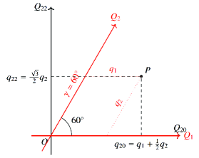
Figure 1: Schematic plot demonstrating the fact that the relation between $q_{20,22}$ and $q_{1,2}$ (33) indicates a tilted axis for $q_{1}$ and $q_{2}$. A quadrupole deformation point “P” is at ($q_{20}$, $q_{22}$), with $Q_{20}$ and $Q_{22}$ being the horizontal and vertical axes ($Q_{20}$-$Q_{22}$ system), respectively. The same point, “P” can be represented in a new system formed by $Q_{1}$ and $Q_{2}$ (differentiated from the $Q_{20}$-$Q_{22}$ system by red color). In this new system, the coordinate ($q_{1}$, $q_{2}$) relates to the coordinate in the $Q_{20}$-$Q_{22}$ system through Eq. (33).

Conventionally, one adds constraints on $q_{20}\equiv\langle\hat{Q}_{20}\rangle$ and $q_{22}\equiv\langle\hat{Q}_{22}\rangle$ moments for quadrupole deformations. However, the hit3d code adds constraints to the $q_{1}$ and $q_{2}$ values. The $q_{1}$ and $q_{2}$ moments are defined to be linked to the $q_{20}$ and $q_{22}$ values through [32]

$$q_{20} =q_{1}+\frac{1}{2}q_{2},$$ (33)

$$q_{22} =\frac{\sqrt{3}}{2}q_{2}.$$

It is customary to define two mass-independent parameters to quantify the degree of quadrupole deformation, namely

$$\beta_{2} =\sqrt{\alpha_{20}^{2}+\alpha_{22}^{2}},$$ (34)

$$\gamma =2\arctan(\frac{\sqrt{3}q_{2}}{\sqrt{(2q_{1}+q_{2})^{2}+3q_{2}^{2}}+2q_{1}+q_{2}}),$$ (35)

with $\alpha_{2\mu}=\frac{\sqrt{5\pi}}{3AR^{2}}q_{2\mu}$, $R=1.2A^{1/3}$ fm.

From Eq. (33), it is clear that if $q_{20}$ and $q_{22}$ form a coordinate system measuring the $x$ and $y$ directions, $q_{1}$ and $q_{2}$ form a system with $q_{1}$ measuring the horizontal direction, $q_{2}$ measuring the direction that is rotated anti-clockwise by $\gamma=60^{\circ}$ with respect to $q_{1}$ direction. For details, see Figure 1.

Table 1: Suppose $a$ is a positive real number, the $q_{1}$ and $q_{2}$ values one needs to take to obtain the typical $\gamma$ values.

$\gamma$	$q_{1}$	$q_{2}$
$+60^{\circ}$	0	$a$
$+30^{\circ}$	$a$	$a$
$0^{\circ}$	$a$	0
$-30^{\circ}$	$2a$	$-a$
$-60^{\circ}$	$a$	$-a$
$-90^{\circ}$	$a$	$-2a$
$-120^{\circ}$	0	$-a$

Compared to the $q_{20}$ and $q_{22}$ values, constraining on the $q_{1}$ and $q_{2}$ values provides more convenient access to the deformation points on the $\gamma=30^{\circ}$ and 60^∘ lines. Indeed, to have a $\gamma=30^{\circ}$ or 60^∘ deformation, one constrains $q_{1}=q_{2}={\rm constant}$ or $q_{1}=0$, $q_{2}={\rm constant}$. For applications breaking the time-reversal symmetry, the deformation points in the sector from $\gamma=0^{\circ}$ to 60^∘ are not sufficient. For example, a cranking calculation in the $y$ direction may require the calculation of total Routhian in the range of $\gamma$ from $-120^{\circ}$ to $60^{\circ}$. Table 1 lists a few typical $\gamma$ values and $(q_{1},q_{2})$ values corresponding to them.

To obtain a potential-energy curve with axial symmetry, one asks for $q_{2}=0$ and varies $q_{1}$ from a negative value to a positive value, which corresponds to a shape varying from an oblate to a prolate deformation. An alternative way to access the oblate deformation is to keep $q_{1}=0$ and increase the $q_{2}$ value to positive numbers. These two methods differ in that the oblate shapes have different orientations in the Cartesian coordinate. To have a triaxial deformation, one needs to constrain the $q_{2}$ to a non-zero value.

2.2.2 The augmented Lagrangian method

In a quadratic penalty method, one minimizes the following total energy

$$E^{\prime}=E+C\quantity(q-q^{0})^{2},$$ (36)

where $q\equiv\langle\hat{Q}\rangle$ and $q^{0}$ is the desired multipole moment introduced in Section 2.2.1. For each different multipole constraint, a term such as that in Eq. (36) is added, and in general, $q$, $q^{0}$, and the associated coefficient $C$ have indices to label the particular moments constrained. If one adds more than one constraint, a summation of terms is assumed. The indexes and summation symbols are ignored here for brevity.

Taking the variational derivative of $E^{\prime}$, one obtains the s.p. Hamiltonian

$$\hat{h^{\prime}}=\hat{h}+2C\quantity(q-q^{0})\hat{Q},$$ (37)

where the parameter $C$ is chosen in such a way that the total constraint energy $E_{\rm mult}\equiv C(q-q^{0})^{2}$ is in the order of a few MeV at the beginning of the iteration.

In general, the quadratic penalty method can constrain the solution to be near the desired value $q^{0}$, but seldomly to $q^{0}$ exactly. The ALM is introduced to the DFT in Ref. [53]. In the ALM, one minimizes the following total energy

$$E^{\prime}=E+L\quantity(q-q^{0})+C\quantity(q-q^{0})^{2}.$$ (38)

Compared to the quadratic penalty method in Eq. (36), the ALM includes a linear term in the total energy in Eq. (38). The s.p. Hamiltonian becomes

$$\hat{h^{\prime}}=\hat{h}+2C\quantity(q-q^{0}(L)),$$ (39)

where $q^{0}(L)=q^{0}-\frac{L}{2C}$. Comparing Eq. (37) and Eq. (39), we see that the ALM requires the targeted multipole moment ($q^{0}$) to be substituted by $q^{0}-\frac{L}{2C}$. However, the $L$ value needs to be updated during the iteration process according to

$$L^{(k+1)}=L^{(k)}+2C\quantity(q-q^{0}).$$ (40)

The iterations can start from a zero value, $L^{(0)}=0$.

Another similar constraining method to the ALM has been used in the Lyon group [32]. The two methods differ in that the targeted moment is updated according to

$$L^{(k+1)}=L^{(k)}-\epsilon_{\rm constr.}\quantity(q-q^{0}),$$ (41)

where $\epsilon_{\rm constr.}$ is a constant between 0 and 1. The two methods turn out to be effective in constraining the nuclear deformations exactly at the desired moment values.

2.3 TDDFT method

This section presents aspects related to the calculations of nuclear dynamics. Since the application areas of the TDDFT method are mostly nuclear vibrations or collisions, the preparations of the initial states in Sec. 2.3.1 are for these two applications. The time evolution of the wave functions is discussed in Sec. 2.3.2. Section 2.3.3 includes comments about the consistencies with the EDFs and pairing treatment of the static calculations. After the time evolution, analysis needs to be performed. For the vibration calculations, we include a discussion about the absorbing boundary conditions in Sec. 2.3.4, the Fourier transform of the response functions in Sec. 2.3.5, and the calculation of the energy-weighted sum rules in Sec. 2.3.6.

2.3.1 Boosting the wave functions

A time-dependent simulation starts with a boost on the static states before time evolution. Two main research areas exist for the TDDFT application, namely, the harmonic vibration of nuclear near the minimum of the potential well and the heavy-ion collision of two nuclei. In this subsection, we discuss the two ways of exciting the two types of modes in the hit3d code.

A. Harmonic vibration

One of the main application areas of the TDDFT is to simulate the harmonic vibrations of a nucleus and analyze the spectrum. One of the most common excitation modes is the isovector dipole resonances. To initiate such a vibration, one applies an instantaneous boost on proton and neutron wave functions in opposite directions. For details, see Ref. [52].

This section discusses how the hit3d code excites multipole vibration modes. Taking the isoscalar quadrupole boosts as an example, we have

$$\phi_{k,q}(\bm{r},\sigma;t=0)=\exp\left[-i\epsilon\,\alpha\,\hat{\mathscr{Q}}_{2,\mu}\right]\phi^{\rm(stat)}_{k,q}(\bm{r},\sigma),$$ (42)

where the constant, $\alpha$, is chosen to be $Z/A$. Similar choice is made in Refs. [55, 56]. The s.p. wave functions resulted from a converged static calculation are denoted with $\phi^{\rm(stat)}$. For the isovector quadrupole boosts, we differentiate protons and neutrons, namely

$$\phi_{k,q}(\bm{r},\sigma;t=0)=\exp\left[-i\epsilon\,\alpha_{q}\,\hat{\mathscr{Q}}_{2,\mu}\right]\phi^{\rm(stat)}_{k,q}(\bm{r},\sigma),$$ (43)

where $\alpha_{n}=-Ze/A$ and $\alpha_{p}=Ne/A$.

After the boosts, the quadrupole moments $q^{\rm IS}_{2\mu}(t)\equiv\expectationvalue*{\alpha\,\hat{\mathscr{Q}}_{2,\mu}}{\Phi(t)}$ and $q^{\rm IV}_{2\mu}(t)\equiv\sum_{q\in\{n,p\}}\expectationvalue*{\alpha_{q}\,\hat{\mathscr{Q}}_{2,\mu}}{\Phi(t)}$ are recorded for the isoscalar and isovector boosts, respectively. These quadrupole moments are later used to perform the Fourier analysis to obtain the strength functions. The current version of the hit3d code allows for the isoscalar and isovector boosts with $(\lambda,\mu)=(2,0),(2,1),(2,2),(3,0),(3,2)$. In addition, it boosts isoscalar monopole [$(\lambda,\mu)=(0,0)$] and isovector dipole ($\lambda=1$) moments.

B. Heavy-ion reactions

To prepare for reaction calculations involving two nuclei, one first places the nuclei at the proper positions before giving them momenta. This is done by the following transformation [29, 4]

$$\phi_{k,q}^{(1)}(\bm{r},\sigma;t=0)=\exp(i\bm{p}_{1}\cdot\bm{r})\,\phi^{\rm(stat)}_{k,q}(\bm{r}-\bm{R}_{1},\sigma),$$ (44a)

$$\phi_{k,q}^{(2)}(\bm{r},\sigma;t=0)=\exp(i\bm{p}_{2}\cdot\bm{r})\,\phi^{\rm(stat)}_{k,q}(\bm{r}-\bm{R}_{2},\sigma).$$ (44b)

In this case, two identical nuclei, denoted with $(1)$ and $(2)$, are placed at $\bm{R}_{1}$ and $\bm{R}_{2}$, respectively. They are boosted from a g.s. indicated by $\phi^{\rm(stat)}$. The resulting two nuclei move with the momenta of $\bm{P}_{1}=A_{1}\bm{p}_{1}$ and $\bm{P}_{2}=A_{2}\bm{p}_{2}$.

Note, that since the wave functions are defined only on the grid points, we can only move nucleus at incremented positions. To place the nuclei at any position, one needs to perform an interpolation procedure. This may end up with an excited HF solution. Hence, the current version of the hit3d code does not have this feature of repositioning the nucleus at any coordinate in the simulating box.

Upon the boosts in Eqs. (42) and (44) being performed, a new compound system is formed. For the nuclear reaction case, the system constitutes two nuclei placed at a distance:

$$\phi_{k,q}(\bm{r},\sigma) =\phi_{k,q}^{(1)}(\bm{r},\sigma),~{}~{}\mbox{for }k=1,...,M,$$

$$\phi_{M+k,q}(\bm{r},\sigma) =\phi_{k,q}^{(2)}(\bm{r},\sigma),~{}~{}\mbox{for }k=1,...,N.$$

The new compound system $\phi(\bm{r},\bm{\sigma})$ is formed by concatenating the s.p. wave function indices of the two displaced systems (44) together. Before performing time advancement, the code performs an orthonormalization for this new system.

2.3.2 The time advancement

The nuclear non-relativistic time-dependent Schrödinger equation reads

$$i\hbar\partialderivative{\phi_{k,q}(t)}{t}=\hat{h}_{q}(t)\phi_{k,q}(t),$$ (45)

where $\hat{h}_{q}$ can be found in Eq. (2.1.7). In this section, the subscript $q$ is ignored for simplicity. The equation (45) has the formal solution

$$\phi_{k}(t)=\hat{\mathscr{U}}(t)\phi_{k}(0)=\hat{T}\exp(-\frac{i}{\hbar}\int_{0}^{t}\hat{h}(t^{\prime})\,dt^{\prime})\phi_{k}(0),$$ (46)

where $\hat{\mathscr{U}}$ is the time-evolution operator, and $\hat{T}$ is the time-ordering operator. To solve the time-dependent problem, one breaks up the total time evolution into $N$ small increments of time $\Delta t$

$$\hat{U}(t,t+\Delta t)=\exp(-\frac{i}{\hbar}\int_{t}^{t+\Delta t}\hat{h}(t^{\prime})\,dt^{\prime}).$$ (47)

The time-evolution operator $\hat{\mathscr{U}}(t)$ can be obtained by consecutive actions of $\hat{U}(t,t+\Delta t)$

$$\hat{\mathscr{U}}(t)=\prod_{n=0}^{N-1}\hat{U}(n\Delta t,(n+1)\Delta t).$$ (48)

For small $\Delta t$ one could approximate $\hat{U}(t,t+\Delta t)$ by Taylor expansion up to order $m$:

$$\exp(-\frac{i}{\hbar}\hat{h}\Delta t)\approx\sum_{n=0}^{m}\frac{1}{n!}\left(\frac{-i\Delta t}{\hbar}\right)^{n}\hat{h}^{n},$$ (49)

where $\hat{h}$ has been assumed to be time independent in the time interval of $\Delta t$. In the current work, $\Delta t$ is taken to be 0.2 fm/$c$, and $m=4$. These choices are motivated by previous TDHF calculations.

In realistic calculations, each time advance of s.p. wave functions $\phi_{k}$, from time $t$ to $t+\Delta t$, has been achieved by using the procedure adopted by the Sky3D code [29, 30]. Specifically, from a series of s.p. wave functions at $t$, $\phi_{k}(t)$, one first performs

$$\phi_{k}^{\rm temp}(t+\Delta t)=\hat{U}^{\rm t}(t,t+\Delta t)\phi_{k}(t).$$ (50)

Having $\phi_{k}^{\rm temp}(t+\Delta t)$, and $\phi_{k}(t)$, one assembles various densities using respective s.p. wave functions, obtaining the $\rho^{\rm temp}(t+\Delta t)$ and $\rho(t)$.

Using these densities, one obtains the densities at a “middle time”, $\rho^{\rm mid}(t+\frac{\Delta t}{2})=0.5[\rho^{\rm temp}(t+\Delta t)+\rho(t)]$. Now, one constructs the Hamiltonian $\hat{h}^{\rm mid}$, using $\rho^{\rm mid}(t+\frac{\Delta t}{2})$ [see Eq. (15) of Ref. [49], and Eq. (2.1.7) for the form of the Hamiltonian]. A second time propagation operation $\hat{U}^{\rm mid}(t,t+\Delta t)$ with $\hat{h}^{\rm mid}$ [Eq. (49)] is performed on the s.p. states, finally obtaining the wave functions at $t+\Delta t$

$$\phi_{k}(t+\Delta t)=\hat{U}^{\rm mid}(t,t+\Delta t)\phi_{k}(t).$$ (51)

Here, $\hat{U}^{\rm mid}$ differs from $\hat{U}^{\rm t}$ [Eq. (50)] in that the former uses the s.p. Hamiltonian in its exponent [Eq. (49)] at the time $t+\frac{\Delta t}{2}$, whereas the latter refers to the operator $\hat{U}$, where the Hamiltonian is constructed using the quantities at the time $t$.

2.3.3 Consistencies in the static and dynamic calculations

As alluded to in the Introduction (1), the hit3d code ensures that the EDFs in static and time-dependent calculations are the same. For the kinetic term (24) in $\hat{h}_{q}$ (2.1.7), the hit3d code switches on or off the center-of-mass correction for static and time-dependent parts together. For the case of harmonic vibrations, careful analyses [57] show that small spurious strength may occur if the consistency is not maintained. In the results presented later in this work, we ignore the center-of-mass correction for both static and dynamic parts. We also note that for collisions where the mass number $A$ is different for the fragments and the combined system, the simple centre-of-mass prescription (24) cannot be used since there is not a single consistent definition of $A$.

When the BCS pairing is included, the occupation amplitudes, $v_{k,q}$’s, are kept unchanged during the time development [29, 30]. When evaluating the densities, the s.p. wave functions vary according to Eq. (45). This is a coarse approximation of dynamical pairing, as the occupation probabilities should vary with time. Indeed, some of the problems associated with the TDHF + BCS method in describing particle transport have been discussed in Ref. [58]. This approximation of the pairing will be improved in our future developements. A natural extension would be to solve the full time-dependent HFB problem [59, 60, 61]. Since the HFB theory treats nuclear interactions in the particle-hole and pairing channels in one single variational process [37], a time-dependent HFB treatment allows for the occupation amplitudes to be determined dynamically by the upper and lower components at a given time.

2.3.4 The absorbing boundary conditions

With Dirichlet boundary conditions, it is known that the TDDFT calculations show the occurrence of non-physical particle densities at the boundary region. To cure this problem, the so-called absorbing boundary conditions (ABC) is proposed [9]. The hit3d code implements such a feature by introducing an imaginary potential

$$\hat{h}(\bm{r})\rightarrow\hat{h}(\bm{r})+i\tilde{\eta}(\bm{r})$$ (52a)

at the boundary region of the form

$$\tilde{\eta}(\bm{r})=\left\{\begin{array}[]{ll}0&\mbox{for }0<|\bm{r}|\leq R\\ \eta_{0}\frac{|\bm{r}|-R}{\Delta r}&\mbox{for }R<|\bm{r}|<R+\Delta r\end{array}\right.\,.$$ (52b)

The ABC method turns out to be effective in absorbing the emitted particles.

2.3.5 The Fourier transform

For harmonic vibrations, after the boost, the nucleus starts to vibrate. The relevant multipole moment $q(t)\equiv\sum_{k}\,v_{k}^{2}\,\langle\phi_{k}(t)|\hat{\mathscr{Q}}|\phi_{k}(t)\rangle$ is recorded as a function of time. A Fourier transform is then performed on $\Delta q(t)\equiv q(t)-q(t=0)$ to obtain the strength function corresponding to $\hat{\mathscr{Q}}$:

$$S(E;\hat{\mathscr{Q}})=-\frac{1}{\pi\hbar\epsilon}{\rm Im}\int\Delta q(t)\,dt\,e^{(iE-\Gamma/2)t/\hbar},$$ (53)

where $\Gamma$ (in MeV) is the smoothing width.

2.3.6 The energy-weighted sum rules (EWSRs)

From the strengths, the EWSR can be calculated using

$$m_{1}=\int E\times S(E)dE.$$ (54)

Recently, the EWSR for the density functional theory has been systematically derived in Refs. [62, 56]. The EWSRs for the IVD operator has been shown in Ref. [52]. For the isoscalar operators considered here, the sum rule using Eq. (62) of Ref. [56] can be adapted as follows

$$m_{1}\quantity(\hat{\mathscr{Q}}_{\lambda\mu})=\frac{\hbar^{2}}{2m}\alpha^{2}\int d\bm{r}\,\quantity(\gradient{\mathscr{Q}_{\lambda\mu}})^{2}\,\rho(\bm{r}),$$ (55)

where $\rho=\rho_{n}+\rho_{p}$, and $m=\frac{1}{2}(m_{n}+m_{p})$.

The EWSR value obtained from Eq. (55) is related to various densities of the g.s. Thus, they can be determined rather precisely. To what extent the $m_{1}$ values obtained from TDDFT [Eq. (54)] and Eq. (55) agree forms a stringent testing ground for the hit3d code.

2.4 Numerical solution of the static and time-dependent problems

As shown in Eq. (2.1.7), the s.p. Hamiltonian of the SHF problem contains systematic derivative operations on the wave functions up to the second order. This can be seen more specifically in B, where the most complicated operation of $\hat{h}_{q}$ on a spinor is specifically expanded. In this section, we present in some detail about the numerical methods used to solve the DFT (2.1) and TDDFT (2.3) problems. In Sec. 2.4.1, we show the way hit3d discretizes the 3D Cartesian space. Section 2.4.2 presents the way hit3d evaluates the first and second derivatives of a function, namely, the finite-difference method used by the code. Finally, the imaginary time step method hit3d code adopts to solve the HF problem is presented in Sec. 2.4.3.

2.4.1 The grid points arrangement

The grid points in the present implementation are moved away from the origin of the simulating box and differs from those of Ref. [49]. Specifically, in the example of one dimension, instead of using a set of coordinates at

$$[-n_{x}^{\rm max},...,0,1,...+n_{x}^{\rm max}]\times dx,$$ (56)

the hit3d code represents the problem on grid points at the coordinates

$$[-n_{x}^{\rm max}+0.5,...,-0.5,0.5,...+n_{x}^{\rm max}-0.5]\times dx,$$ (57)

where $n_{x}^{\rm max}$ is an integer enumerating the points at the edge of the simulating box. $dx$ denotes the grid spacing. Note that the latter choice (57) has an even number of grid points, whereas the former one (56) has an odd number of grid points. This choice is guided by the fact that the inclusion of the grid point at the origin of the box results in numerical problems [29]. Using the grid shown in Eq. (57), the integration can be carried out by summation on the grid, without the interpolation as presented in Ref. [49].

2.4.2 Derivatives on the grid points

Table 2: The finite-difference coefficients for the first-order ($c_{m}$) and second-order ($d_{m}$) derivatives. For the first derivatives, we use a seven-point central formula (Eq. (58a)). Whereas for the second derivatives, we use a nine-point formula (58b).

$k$	$i-4$	$i-3$	$i-2$	$i-1$	$i$	$i+1$	$i+2$	$i+3$	$i+4$
$c_{m}$	$-$	$-\frac{1}{60}$	$+\frac{9}{60}$	$-\frac{45}{60}$	0	$+\frac{45}{60}$	$-\frac{9}{60}$	$+\frac{1}{60}$	$-$
$d_{m}$	$-\frac{9}{5040}$	$+\frac{128}{5040}$	$-\frac{1008}{5040}$	$+\frac{8064}{5040}$	$-\frac{14350}{5040}$	$+\frac{8064}{5040}$	$-\frac{1008}{5040}$	$+\frac{128}{5040}$	$-\frac{9}{5040}$

The hit3d code uses the finite difference (FD) formulae to approximate the derivatives of various densities and wave functions. We use the seven- and nine-point formulae to approximate the first and second derivatives at $x_{i}=(i-0.5)\times dx$, respectively:

$$f^{\prime}(x_{i})\approx\frac{1}{dx}\sum_{k=i-3}^{i+3}c_{k}f(x_{k}),$$ (58a)

and

$$f^{\prime\prime}(x_{i})\approx\frac{1}{dx^{2}}\sum_{k=i-4}^{i+4}d_{k}f(x_{k}).$$ (58b)

The $c_{k}$ and $d_{k}$ values are listed in table 2.

The values of the function outside the simulating box are unknown. To calculate the derivatives at the border region, we set the values outside the box to be zero. That is, we use the Dirichlet boundary condition for solving the static and time-dependent problems.

Although the FD method is simple, it turns out to be fairly accurate. In Section 3.1.1, we will demonstrate that, from the lighter (⁴⁸Ca) to the heaviest (²⁰⁸Pb) doubly magic nuclei, the method overbinds by only $\sim 0.1\%$ of the total binding energy with $dx=1.0$ fm. It has to be mentioned that such a simple method provides a base for further refinements, such as the Lagrangian interpolation method [32] or a Fourier transformation method [29, 30].

2.4.3 Imaginary time step method

To solve the nonlinear HF problem presented in Eq. (2.1.7), one can expand the Hamiltonian on a basis and diagonalize it. For the nuclear HF problem where only a few tens of s.p. levels are occupied, one finds the imaginary time step method introduced in Ref. [63] to be quite efficient.

The imaginary time step method includes two steps to advance the variation process until the convergence of the nonlinear HF problem. First, one evaluates the following transformed s.p. wave functions

$$\Phi_{k}^{(i+1)}(\bm{r}\sigma)=\Bigg{(}1-\frac{\delta t}{\hbar}\hat{h}\Bigg{)}\,\phi_{k}^{(i)}(\bm{r}\sigma).$$ (59)

The indexes $(i)$ label the iteration number. Note, that $\Phi_{k}^{(i+1)}$’s are not orthonormal now. Second, one performs a Gram-Schmidt procedure to orthonormalize $\Phi_{k}^{(i+1)}$’s, obtaining the $\phi_{k}^{(i+1)}$ for the $(i+1)$-th iteration.

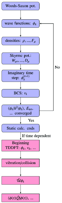
Figure 2: A flowchart demonstrating the main procedures the hit3d code takes to solve the nuclear (TD)DFT problem.

We end this section by summarizing the procedures that the hit3d program adopts to solve the static and time-dependent problems. In Fig. 2, we provide a flowchart to facilitate the explanation.

• The calculation starts by solving the 3D Schrödinger equation with a triaxially deformed Woods-Saxon (WS) potential . Optionally, the code can read the s.p. wave functions recorded on a file. The s.p. wave functions can be solutions to the same static problem but with a nearby deformation.

• Retaining the requested number of neutron and proton wave functions, hit3d computes the densities (9) and potentials (23).

• With the s.p. Hamiltonian, one obtains the s.p. energies and the sum of the fluctuations of each s.p. orbital, weighted by their occupation probabilities [32]

  $$\frac{1}{A}\sum_{k}v_{k}^{2}\Delta\epsilon_{k}^{2}=\frac{1}{A}\sum_{k}v_{k}^{2}\Big{(}\langle\phi_{k}|\hat{h}^{2}|\phi_{k}\rangle-\langle\phi_{k}|\hat{h}|\phi_{k}\rangle^{2}\Big{)}.$$ (60)

• The HF iteration starts by evolving the s.p. wave functions using an imaginary time step method. For this and the last step, one needs to evaluate $\hat{h}\phi_{i}$. In B, we include how this is performed for the most complicated term ($\bm{D}$-term) in Eq. (2.1.7).

• If the differences in total energies, weighted fluctuation sums (60), and quadrupole moments between consecutive iterations are small enough, the static calculation is considered to be converged.

• After obtaining a set of orthonormal wave functions upon convergence, one performs spatial boost on the s.p. wave functions (42-44).

• The time-dependent evolution (46) is then performed on the s.p. wave functions. The quadrupole moments are recorded for the Fourier transformation (53).

3 Comparisons with other codes

3.1 Static cases

In this section, we present a set of static calculations using the hit3d code. For the non-constrained DFT calculations, comparisons are made with the Sky3D codes (Sec. 3.1.1). For the constrained DFT + BCS calculations in Sec. 3.1.2, we use the ALM method to obtain the results with two deformation points for the ¹¹⁰Mo nucleus. The hit3d results are compared with those of the Ev8 code. For these static calculations, the T44 EDF is adopted without center-of-mass correction.

3.1.1 DFT Results without constraint

Table 3: The total ($E_{\rm tot}$), kinetic ($E_{\rm Kin.}$), Coulomb ($E_{\rm Coul}$), tensor ($E_{J^{2}}$), and the Skyrme energies without the tensor contributions ($E_{\rm Skyrme}$) of ⁴⁸Ca, ¹³²Sn, and ¹³²Pb calculated with the T44 parameter [41]. The results calculated using the Sky3D [29, 30] code are also included. The energies are in MeV. The center-of-mass correction [the (1-1/$A$) factor in Eq. (24)] is not included in these calculations.

Nuclei		hit3d				Sky3D
		$dx=1.2$	$dx=1.0$	$dx=0.8$	$dx=0.6$	$dx=0.6$
48Ca	$E_{\rm tot}$	$-$401.034	$-$400.753	$-$400.759	$-$400.816	$-$400.845
	$E_{\rm Kin.}$	837.996	837.251	837.028	837.075	837.103
	$E_{\rm Coul}$	71.156	71.066	71.035	71.029	71.024
	$E_{\rm Skyrme}$	$-$1314.619	$-$1313.568	$-$1313.352	$-$1313.461	$-$1313.518
	$E_{\rm J^{2}}$	4.434	4.498	4.529	4.542	4.545
132Sn	$E_{\rm tot}$	$-$1085.306	$-$1083.747	$-$1083.556	$-$1083.632	$-$1083.709
	$E_{\rm Kin.}$	2463.306	2460.134	2459.179	2459.115	2458.973
	$E_{\rm Coul}$	341.977	341.706	341.602	341.578	341.556
	$E_{\rm Skyrme}$	$-$3909.377	$-$3904.614	$-$3903.469	$-$3903.498	$-$3903.420
	$E_{\rm J^{2}}$	18.788	19.029	19.134	19.171	19.182
208Pb	$E_{\rm tot}$	$-$1619.901	$-$1617.209	$-$1616.681	$-$1616.692	$-$1616.769
	$E_{\rm Kin.}$	3893.725	3889.133	3887.414	3887.170	3887.226
	$E_{\rm Coul}$	798.737	798.150	797.913	797.862	797.809
	$E_{\rm Skyrme}$	$-$6332.832	$-$6325.205	$-$6322.822	$-$6322.571	$-$6322.660
	$E_{\rm J^{2}}$	20.469	20.714	20.814	20.848	20.856

In this section, the ground-state energies of a few spherical nuclei are calculated using the hit3d and Sky3D codes. Special attention has been paid to the convergence of the energies with respect to the grid spacing as well as the contributions due to the time-even part of the tensor contribution.

Table 3 lists the calculated total energies and the decompositions of ⁴⁸Ca, ¹³²Sn, and ²⁰⁸Pb. The tensor contributions are nonzero with the T44 EDF used for these nuclei. For the hit3d and Sky3D codes, the sizes of the simulating boxes have been chosen to be big enough so that the densities at the edge are lower than $10^{-7}$ fm^-3.

First, we discuss the performance with the hit3d code (the first four columns of Table 3). For ⁴⁸Ca, the total energy with $dx=1.2$ fm is overbound by a few hundreds of keV compared to the results with $dx=0.6$ fm. With $dx=1.0$ fm, the total energies are close to those with $dx=0.6$ fm ($\sim 100$ keV) for ⁴⁸Ca and ¹³²Sn. For ²⁰⁸Pb, using $dx=1.0$ fm overbinds the converged total energy by $\sim 500$ keV. Decreasing $dx$ to 0.8 or 0.6 fm, we see the total energies of these three nuclei converge rather well, with the total energies changing by $<100$ keV, indicating good convergence at $dx=0.8$ fm for the heavies nucleus ²⁰⁸Pb. To summarize, for the lighter or medium heavy nuclei with $A<132$, it is adequate to use a grid spacing of $dx=1.0$ fm. Whereas for even heavier nuclei with $A>208$, it is necessary to use a finer grid spacing of $dx=0.8$ fm if one needs better-converged g.s. energies.

We compute the three nuclei using the Sky3D code, listed in the last column in Table 3. For ⁴⁸Ca, these two methods are converged/saturated with respect to the respective model parameters. We notice good agreement among the two sets of calculated results. Indeed, the differences in total energies are smaller than 50 keV, which is only $\sim 0.02\%$ of the total energy. This marks the limit of the comparability of these two codes. For heavier nuclei, we notice that the differences among different codes are about $0.02\%$ of the respective energies.

It is interesting to note that the kinetic energy agrees rather well between hit3d and Sky3D codes. At $dx=0.6$ fm, the differences are only a few tens of keV for the three nuclei. This is impressive because the kinetic energy depends on the Laplacian operation of the s.p. wave functions. The agreement of the kinetic energy indicates that the wave functions are rather close between the two codes.

3.1.2 Constrained DFT Results

Table 4: The calculated total energies ($E_{\rm tot}$) and its decompositions of the kinetic ($E_{\rm Kin}$), Coulomb ($E_{\rm Coul.}$), tensor ($E_{\rm J^{2}}$) energies, and the Skyrme energies minus tensor contributions ($E_{\rm Skyrme}$) of ¹¹⁰Mo calculated using T44 EDF. The pairing energies and pairing gaps ($\Delta_{n,p}$) are also included. The first two columns correspond to the constraint calculations with the targeting quadrupole moments of $(q_{1},q_{2})=(200,200)$ fm². The last two columns correspond results with desired $(q_{1},q_{2})=(600,400)$ fm². The first and third columns are hit3d results; the second and fourth columns are Ev8^τ results. Both codes use a grid spacing of $dx=0.8$ fm. For the pairing strengths, both codes use $V_{n,p}=-500$ MeV fm³. All values are in MeV, except for the $q_{1,2}$ values, the latter of which are in fm².

	hit3d	Ev8τ	hit3d	Ev8τ
$E_{\rm tot}$	$-$896.986	$-$897.111	$-$898.041	$-$898.136
$E_{\rm Kin.}$	1985.011	1990.244	2000.360	2005.029
$E_{\rm Coul.}$	252.435	252.669	250.93	251.112
$E_{\rm Skyrme}$	$-$3122.763	$-$3127.839	$-$3151.848	$-$3155.745
$E_{\rm J^{2}}$	5.158	5.295	9.230	9.353
$E_{\rm pair}^{n}$	$-$12.613	$-$13.163	$-$4.649	$-$5.456
$E_{\rm pair}^{p}$	$-$4.214	$-$4.318	$-$2.064	$-$2.429
$\Delta_{n}$	1.734	1.757	1.029	1.1075
$\Delta_{p}$	1.109	1.119	0.774	0.8364
$q_{1}$ (fm2)	200.054	200.109	600.070	600.135
$q_{2}$ (fm2)	199.942	200.187	399.868	399.590

Table 4 lists the results of ¹¹⁰Mo calculated using two constraint methods: the hit3d and Ev8^τ codes . Comparing the hit3d results with the Ev8^τ results, it can be seen that the total energies agree on the level of 0.1 MeV, although the kinetic energies differ by about 5 MeV. The differences in the kinetic energies using different codes are well known [32]. Note that the two codes give similar pairing properties (pairing gaps and energies).

For the constraining calculations in Table 4, it can be seen that both codes obtain the desired solution at the desired quadrupole moments. The calculated $q_{1,2}$ values deviate from the targeted values by only $<0.2$ fm².

The constrained calculations frequently suffer from divergence. To increase the chance of reaching convergence, we add a few tips when running the code:

• Start the calculation with a set of s.p. wave functions, resulted from the WS potential with the $basis$ deformation that corresponds to the desired quadrupole moments.

• The constraining coefficients (36) of relevant constraining terms need to be chosen in such a way that the constraint energies (36) are not too high, with $E_{\rm constr.}=\sum_{\lambda\mu}C_{\lambda\mu}\quantity(q_{\lambda\mu}-q^{0}_{\lambda\mu})^{2}<10$ MeV.

• If a constraint calculation is successful, use this set of wave functions as a starting point for the constraint calculation for a nearby deformation.

• Use a large mixture of densities from the last iteration. This will tend to slow down the convergence but increase the chance of convergence.

3.2 Dynamic cases

3.2.1 Harmonic Vibrations

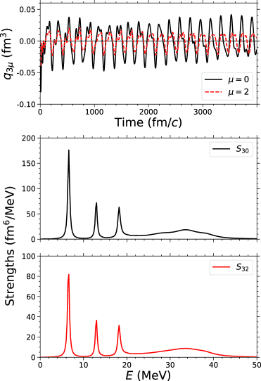
Figure 3: The isoscalar octupole ($\lambda=3$, $\mu=\{0,2\}$) vibrations calculations for ¹⁶O. The upper panel shows the octupole moments as a function of time. The lower two panels display the strengths functions for the $\mu=\{0,2\}$ vibration modes.

Figure 3 plots the results for the harmonic isoscalar octupole vibration of ¹⁶O using the SkM* force. Figure 3(a) plots the octupole moments up to $t=4000$ fm/$c$ after the isoscalar octupole boosts (strength $\epsilon=0.0001$ fm^-3) with $\mu=0,2$ at $t=0$. It can be seen that the magnitudes are maintained.

Fourier transformations are performed on the response functions (53) of the octupole moments, obtaining the strengths of the $q_{30}$ and $q_{32}$ modes, which are displayed in Figs. 3(b) and (c), respectively. Strong narrow peaks at 6.6, 13.0, and 18.2 MeV can be seen, suggesting good harmonic vibrations with phonon energies of $\sim$6.5 MeV. These correspond to the isoscalar $Q_{30}$ and $Q_{32}$ modes. The lowest peaks are the strongest. This seems to be confirmed by the experimental data, where a few lowest negative-parity states (with $I^{\pi}=1^{-}$ and 3^-) appear near $E_{x}\sim 6$ to 9 MeV [65]. In the energy interval of $E\sim[25,45]$ MeV, there are broad continuum strengths corresponding to these octupole modes.

Table 5: EWSR of a few doubly magic nuclei obtained for g.s. and the TDDFT calculation using SkM* force.

Nuclei	Modes	ISM	IVD	ISQ ($\mu=0$)	ISQ ($\mu=2$)	ISO ($\mu=0$)	ISO($\mu=2$)
	unit	fm4MeV	$e^{2}$fm2MeV	fm4MeV	fm4MeV	fm6MeV	fm6MeV
16O	g.s.	9908.0	75.8	492.8	246.4	11891.8	5948.1
	TDDFT	9863.0	75.8	491.1	245.6	11840.9	5920.1
24Mg	g.s.	18666.6	117.1	1161.9	347.5	34738.4	13228.7
	TDDFT	18601.0	116.2	1158.1	346.4	34594.2	13173.3
40Ca	g.s.	38904.2	197.8	1934.9	967.5	67277.6	33658.5
	TDDFT	38513.8	196.3	1928.3	964.0	66997.9	33515.0
48Ca	g.s.	50422.9	234.9	1741.9	870.6	63975.2	32010.6
	TDDFT	50278.7	232.6	1737.8	867.5	63698.6	31867.5
208Pb	g.s.	534222.7	1031.6	16517.8	8258.9	1373619.5	687306.1
	TDDFT	534972.0	1023.2	16460.8	8233.4	1365840.0	684045.0

Table 5 lists the EWSR calculated using the g.s. densities (55) compared with those resulting from a TDDFT-calculated strengths function (54) for a few nuclei. A good agreement can be seen for all the modes that allowed for the hit3d code.

3.2.2 Heavy-ion Collisions

When two ¹⁶O collide, with certain center-of-mass kinetic energy, which is larger than the Coulomb barrier between them, the two nuclei fuse. With higher center-of-mass energy, the two nuclei will separate into two. The threshold energy (the highest center-of-mass kinetic energy at which the fuse happens) is sensitive to the included Skyrme terms. Consequently, it has been customarily used as a benchmark when new terms are added to the TDDFT applications for nuclear reactions [10, 15].

Table 6 lists the threshold energy for the two head-on (with $b=0$) colliding ¹⁶O nuclei. Comparing the results calculated using hit3d with the results using Sky3D code [15], we see a systematic underestimation of the threshold of hit3d results by $\sim 1$ to 2 MeV [15]. It has to be noted that the differences become smaller (by $\sim 1$ MeV) if the Sky3D uses similar grid spacings and colliding angles as those adopted by the hit3d code.

Table 6: The threshold energies for the head-on ¹⁶O-¹⁶O collision ($b=0$) calculated using the TDDFT code hit3d with different forces. The SLy5T is the force fitted for the shell evolutions [13].

Force	Threshold (MeV)
SkM* (full)	72
SLy5T[13]	69
T12	60
T22	64
T26	80
T44	77
T46	85
T64	85
T66	91

4 Input description

The input parameters are included in two files. The header file headers.tensor.108.h contains those parameters fixed at the compilation stage. While the input file input_118.dat contains parameters sent to the executable file.

4.1 Header file

The parameters inside the header file headers.tensor.108.h are fixed at the compilation stage. They can stay unchanged for one mode of calculation.

• HOshell_: the largest $n$ for the Hermite functions used to expand the WS Hamiltonian.

• Spcing: the grid spacing ($dx,dy,dz$) fm for both the HF and TDDFT calculations.

• delta_t: the step size of the imaginary time [$\delta t$ in Eq. (59)] in units of 10^-22 s. A large $\delta t$ leads to divergence of the HF problem since we expand the exponent up to the first order in Eq. (59). With $dx=1.0$ fm, it is found that $\delta t=0.04$ leads to divergence. We use a much smaller $\delta t=0.005$ to ensure convergence for grid spacings ranging from 0.6 to 1.2 fm. Static calculations with smaller grid spacings require even smaller $\delta t$ to achieve convergence.

• Rab, dRab, and eta_0: the $R$, $\Delta r$, and $\eta_{0}$ parameters for the ABC (52).

• Nx_max: this parameter specifies the largest $N$ quantum number in the $x$ direction of the 3D HO wave functions expanding the WS Hamiltonian. The actual largest value is Nx_max-1.

• Ny_max, Nz_max: similar to Nx_max, except for the $y$, and $z$ directions.

• N: the number of ($n_{x}$, $n_{y}$, $n_{z}$) points for the WS potential.

• beta2_ws: the $\beta_{2}$ deformation of the WS potential.

• gamma_ws: the $\gamma$ deformation of the WS potential.

• max_x, xo: xo and max_x-1 specify the left-most and right-most points in the $x$-axis. Specifically, the coordinate on the left-most is (xo-0.5)$\times$Spcing. On the right-most is (max_x-1.5)$\times$Spcing.

• max_y, yo: similar to max_x and xo, except in the $y$ direction.

• max_z, zo: similar to max_x and xo, except in the $z$ direction.

4.2 Input file

The data file input_118.dat contains input parameters for the executable file to read. The program reads the file line by line. The meaning of the lines is determined by the order they appear in the data file. Thus, no line can be omitted, and the order of the lines needs to be kept. For most lines, the first keywords are there to remind the user what they are changing. The program reads the data after the keywords. This section discusses all the parameters in the data (input_118.dat) file.

• NZ: after this keyword, two real numbers are given to indicate the neutron and proton numbers of the nucleus to be calculated. We take an integer of the two real numbers. If the resulting integers are both even, the TDDFT + BCS calculation will be performed. If either or both of the two integers is/are odd, BCS is switched off.

• N_wf: two integers are provided to indicate the number of wave functions for the neutrons and protons, respectively. They should be larger than the neutron and proton numbers, respectively.

• Force: a string is provided to indicate the force name.

• pair_type: an integer is provided. “0” for delta force; “1” for mixed pairing (19).

• v0n: the neutron pairing strength (19). It is in the unit of MeV fm³

• v0p: similar to v0n, except for proton pairing strength.

• tensor_on: an integer is provided after this keyword. If it is “0”, then the tensor contribution in Eq. (15) is ignored. Specifically, we set $b_{14,15,16,17}$ to be zero. If it is “1”, then the tensor contribution in the form of Eq. (2.1.7) is included. If it is “2”, then the last term in Eq. (2.1.7) is calculated using Eq. (63) from Ref. [43], see B.

• st_on: an integer is provided. If it is “0”, the terms inside the same bracket as $\bm{s}\dotproduct\bm{T}$ in the EDF (15) are not included. Specifically, we set $b_{14}$ and $b_{15}$ to be zero. If it is “1”, those terms are included.

• sf_on: similar to st_on, except for the terms inside the same bracket as $\bm{s}\dotproduct\bm{F}$ in the EDF (15).

• the line after sf_on contains an integer followed by a file name. If the integer is “1”, the static run will be restarted from the wave functions in the file with the filename provided after the “1” in this line. If the integer is “0”, the run will start without reading information from another file. Instead, it will start by calculating the WS wave functions.

• this line, which is before vibration, contains an integer followed by a file name. If the integer is “1”, the s.p. wave functions of the current static run will be written in the file with the file name provided after the “1” in this line. If the integer is “0”, the information will not be saved.

• vibration: an integer is provided after this keyword. If it is “1”, the time-dependent calculation will be performed for a harmonic vibration [isoscalar boost (42)]. If it is “2”, the isovector boost (43) will be performed. If it is “0”, the time-dependent vibration calculation will not be performed. The mode is specified with the ExcMod keyword.

• ExcMod: an integer is provided after this keyword to select the vibration mode to excite. The integers “0”, “1”, “20”, “21”, “22”, “30”, and “32” are available to excite the isoscalar monopole, isovector dipole, isoscalar/isovector quadrupole ($\mu=0,2$), and octupole ($\mu=0,2$) vibrations, respectively. For the last five modes, to specify the isoscalar or isovector vibration, one can refer to the vibration keyword.

• kick_xyz: an integer is provided after this keyword. If “1” is provided, the isovector dipole vibration is in the direction of $(\hat{\bm{x}},\hat{\bm{y}},\hat{\bm{z}})$. If “0” is provided, the isovector vibration is only in the $z$ direction. This keyword does not concern other modes except for the isovector dipole vibration.

• epsilon_monopole: the boost parameter $\epsilon$ (in fm^-2) for the isoscalar monopole vibration.

• epsilon_quadrupole: the boost parameter $\epsilon$ (in fm^-2) for the isoscalar/isovector quadrupole vibrations.

• epsilon_dipole: the boost parameter $\epsilon$ (in fm^-1) for the isovector dipole vibration.

• epsilon_octupole: the boost parameter $\epsilon$ (in fm^-3) for the isoscalar/isovector octupole vibrations.

• collision: an integer is provided after the keyword.

  • If “0” is provided, the collision calculation will not be performed.

  • If “1” is provided, the calculation will compute a testing case where the nucleus from the static run will be replaced at a new position (see frag_one) and boosted across the box.

  • If “2” is provided, the same two nuclei calculated from the static run will be duplicated to two positions (see frag_one and frag_two to specify positions) and boosted.

  • If “3” is provided, the first nucleus will be from the current static run. The second colliding nucleus will be read from a file specified in the next line.

• the line after keyword collision contains an integer and a file name. If the previous line collision is “3”, then the integer in this line has to be “1”. Meanwhile, the input with the given file name has to be supplied. If the integer in the previous line is not “3”, then the integer of this line can be “0”. In this case, the file name of this line is ignored.

• E_cm: the total kinetic energy plus the Coulomb energy for the two colliding nuclei. It is in the unit of MeV.

• frag_one: three real numbers are provided to indicate the position ($x_{1},y_{1},z_{1}$) of the first nucleus. They are in the unit of fm.

• frag_two: the same as frag_one, except for the position of the second nucleus.

• TaylorExp: an integer number, “4” or “6”, is provided to specify the order of the Taylor expansion $m$ in Eq. (49).

• delta_t: a real number (in the unit of fm/$c$) is provided to specify the time step for TDDFT calculations in Eq. (49). This is to be distinguished from the time step in the imaginary time step method, delta_t, which is in the header file.

• max_ite: an integer is provided to specify the maximum iteration number for the static calculation.

• itmax: an integer is provided to specify the largest number of time steps for the TDDFT calculations.

• nprint: an integer is provided. The report for the static calculation is printed every nprint iterations. The table for dynamic information is printed every 20$\times$nprint time steps.

• threshold: a small real number (close to zero) is provided to specify the threshold energy (in MeV). If the energy difference between this iteration and the last iteration is smaller than it for five consecutive iterations, then the static calculation is terminated if other thresholds are also reached, see below.

• threshold_q1t: a threshold value for $q_{1}$ (in fm²) is provided after the keyword. If the difference in $q_{1}$ between the two consecutive iterations is smaller than it, the convergence is reached.

• threshold_q2t: similar to threshold_q1t but for the $q_{2}$ value.

• threshold_disp: similar to threshold_q1t but for the threshold of fluctuation (60).

• alpha_mix: a real coefficient between 0 and 1 is provided to multiply with the densities from the last iteration. Only (1-alpha_mix) of the current iteration is taken to the next iteration.

• nfree: an integer is provided. After nfree number of iterations, the constraints on the $q_{1}$ and $q_{2}$ quadrupole moments will be removed.

• C1t: two real numbers need to be provided. The first one is the quadratic constaint coefficient (in MeV fm^-4) in Eq. (36) for the $q_{1}$ quadrupole moment defined in Eq. (33). The second real number specifies the desired $q_{1}$ value (in fm²).

• C2t: the same as C1t, except for the $q_{2}$ values defined in Eq. (33).

• C30t: the same as C1t, except for $q_{30}$ (in fm³) defined in Eq. (31). It is in the unit of MeV fm^-6.

• C31t: the same as C30t, except for $q_{31}$.

• C32t: the same as C30t, except for $q_{32}$.

• C33t: the same as C30t, except for $q_{33}$.

• C10x: three real numbers need to be provided after this keyword. The first one is the quadratic constraint coefficient (in MeV fm^-2) for the $q_{x}$ moment (28). The second and the third are the desired $q_{x}$ value (in fm) one aims to calculate for neutrons and protons, respectively.

• C10y: the same as C10x, except for the $q_{y}$ moment.

• C10z: the same as C10x, except for the $q_{z}$ moment.

• Cxy: similar to C10x, except for the $q_{xy}$ moment (29). The coefficient is in MeV fm^-4, and the $q_{xy}$ moments are in fm².

• Cyz: the same as Cxy, except for the $q_{yz}$ moment.

• Czx: the same as Cxy, except for the $q_{xz}$ moment.

• epscst: a real number ranging from 0 to 1.0 is specified. It is to be multiplied by the updated $L$ [$\epsilon_{\rm constr.}$ in Eq. (41)]. epscst is for $q_{1}$ and $q_{2}$ updates.

• epscst_q3: similar to epscst, except for updates on octupole moments.

• epscst_cent: similar to epscst, except for updates on the $q_{x,y,z}$ moments.

• epscst_refl: similar to epscst, except for updates on the $q_{xy,yz,zx}$ moments.

• ral: a real number ranging from 0 to 1.0 is specified. It is to be multiplied by the potentials (39) due to the linear constraints on the moments that are intrinsic deformation, $q_{1}$, $q_{2}$, $q_{30}$, and $q_{32}$.

• rall: a real number is provided after the keyword, which is similar to ral except for the moments that are responsible for the center of mass and the orientation of the nucleus.

• in the line after rall, a file name is provided to record the multipole moments as a function of time. At the end of this file, the strengths associated with this vibration mode are saved as a function of energy.

• the last line of the data file contains a file name to save the various energies originating from the energy functional (15) as functions of time.

5 Acknowledgments

The current work is supported by National Natural Science Foundation of China (Grant No. 12075068 and No. 11705038), the UK STFC under grant No. ST/P005314/1, ST/V001108/1, JSPS KAKENHI Grant No. 16K17680, and No. 20K03964.

Appendix A Relationships between $\{t,x\}$ and $\{b\}$ coefficients

In this section, we connect the $\{b\}$ coefficients in Eq. (2.1.4) with the $\{t,x\}$ coefficients used to define the Skyrme force [35]. In the hit3d code, the interconnection between $\{b\}$ and ${t,x}$ coefficients are mediated by the $\{a\}$ coefficients that appeared in Ref. [43].

Specifically, the ${t,x}$ coefficients are first transformed to $\{a\}$ coefficents:

$$a_{1} =\frac{t_{0}}{2}\quantity(1+\frac{x_{0}}{2}), a_{2} =-\frac{t_{0}}{2}\quantity(x_{0}+\frac{1}{2}),$$

$$a_{3} =\frac{t_{0}x_{0}}{4}, a_{4} =-\frac{t_{0}}{4},$$

$$a_{5} =\frac{1}{4}\quantity(t_{1}+t_{2}+\frac{t_{1}x_{1}+t_{2}x_{2}}{2}), a_{6} =\frac{1}{16}\quantity(t_{2}-3t_{1}-\frac{3t_{1}x_{1}}{2}+\frac{t_{2}x_{2}}{2}),$$

$$a_{7} =\frac{3}{2}\quantity(t_{2}x_{2}-t_{1}x_{1}), a_{8} =\frac{1}{32}\quantity(t_{2}+3t_{1}),$$

$$a_{9} =\frac{1}{16}\quantity(3t_{1}x_{1}+t_{2}x_{2}), a_{10} =\frac{1}{8}\quantity(t_{1}x_{1}+t_{2}x_{2}),$$

$$a_{11} =\frac{1}{8}\quantity(t_{2}-t_{1}), a_{12} =\frac{1}{4}\quantity(t_{2}x_{2}-t_{1}x_{1}),$$

$$a_{13} =\frac{t_{3}}{12}\quantity(1+\frac{x_{3}}{2}), a_{14} =-\frac{t_{3}}{12}\quantity(x_{3}+\frac{1}{2}),$$

$$a_{15} =\frac{t_{3}x_{3}}{12}, a_{16} =-\frac{t_{3}}{12},$$

$$a_{17} =\frac{W_{0}}{2}, a_{18} =\frac{W_{0}}{2}.$$

For tensor part of the Skyrme EDF, the relations between $\{a\}$ and $\{t,x\}$ coefficients are

$$a_{19} =\frac{3}{16}\quantity(3t_{e}-t_{o}), a_{20} =-\frac{3}{16}\quantity(3t_{e}+t_{o}),$$

$$a_{21} =-\frac{1}{4}\quantity(t_{e}+t_{o}), a_{22} =\frac{1}{4}\quantity(t_{e}-t_{o}),$$

$$a_{23} =\frac{3}{4}\quantity(t_{e}+t_{o}), a_{24} =-\frac{3}{4}\quantity(t_{e}-t_{o}),$$

$$a_{25} =\frac{1}{16}\quantity(3t_{e}-t_{o}), a_{26} =-\frac{1}{16}\quantity(3t_{e}+t_{o}).$$

The ${b}$ coefficients are related to the ${a}$ coefficients through

$$b_{1} =a_{1}, b_{2} =a_{2},$$

$$b_{3} =a_{5}, b_{4} =a_{11}+a_{12},$$

$$b_{5} =a_{6}, b_{6} =a_{8}+a_{9},$$

$$b_{7} =a_{13}, b_{8} =a_{14},$$

$$b_{9} =a_{17}, b_{9q} =a_{18},$$

$$b_{10} =a_{3}, b_{11} =a_{4},$$

$$b_{12} =a_{15}, b_{13} =a_{16},$$

$$b_{14} =-a_{21}-a_{10}, b_{15} =-a_{22}-a_{11},$$

$$b_{16} =-\frac{1}{2}a_{23}, b_{17} =-\frac{1}{2}a_{24},$$

$$b_{18} =a_{25}, b_{19} =a_{26},$$

$$b_{20} =a_{19}, b_{21} =a_{20}.$$

Note that for $b_{14}$ and $b_{15}$, contributions from $t_{1}$ and $t_{2}$ can be seen (through $a_{10}$ and $a_{11}$) [43]. This means that even if the tensor force is ignored ($t_{o}=t_{e}=0$), contributions due to $\bm{s}\dotproduct\bm{T}$ terms in Eq. (15) appear in the Skyrme EDF. Therefore, ideally, st_on should be turned on even for the EDFs without tensor interaction. However, only a few parameter sets include the $\bm{s}\dotproduct\bm{T}$ terms in the fitting process. The common practice has been to ignore these complicated terms. Consequently, the users are advised to switch them off to save running time, especially for the EDFs without tensor interactions included in the fitting procedure.

Appendix B The last term in Eq. (2.1.7)

Now, we specifically expand the last two terms in Eq. (2.1.7):

$$-\gradient\dotproduct\quantity[\hat{\bm{\sigma}}\dotproduct\bm{C}]\gradient\matrixquantity(\phi_{\uparrow}\\ \phi_{\downarrow})$$

$$=-\quantity[\gradient\quantity(\hat{\bm{\sigma}}\dotproduct\bm{C})]\dotproduct\gradient\matrixquantity(\phi_{\uparrow}\\ \phi_{\downarrow})-\quantity(\hat{\bm{\sigma}}\dotproduct\bm{C})\nabla^{2}\matrixquantity(\phi_{\uparrow}\\ \phi_{\downarrow})$$ (61)

and

$$-\gradient\dotproduct\bm{D}\hat{\bm{\sigma}}\dotproduct\gradient\matrixquantity(\phi_{\uparrow}\\ \phi_{\downarrow})$$

$$=-\quantity(\gradient\dotproduct\bm{D})\quantity[\hat{\sigma}_{x}\gradient_{x}\matrixquantity(\phi_{\uparrow}\\ \phi_{\downarrow})+\hat{\sigma}_{y}\gradient_{y}\matrixquantity(\phi_{\uparrow}\\ \phi_{\downarrow})+\hat{\sigma}_{z}\gradient_{z}\matrixquantity(\phi_{\uparrow}\\ \phi_{\downarrow})]$$

$$\quad-\bm{D}\dotproduct\gradient\quantity[\quantity(\hat{\bm{\sigma}}\dotproduct\gradient)\matrixquantity(\phi_{\uparrow}\\ \phi_{\downarrow})].$$ (62)

Another form of the $b_{16},b_{17}$ term is obtained in Barton’s thesis [43] [Eq. (2.4.8)], which reads

$$-\frac{1}{2}\sum_{\mu\nu}\hat{\sigma}_{\nu}\quantity[(\nabla_{\nu}D_{q,\mu})\nabla_{\mu}+2D_{q,\mu}\nabla_{\nu}\nabla_{\mu}+(\nabla_{\mu}D_{q,\mu})\nabla_{\nu}].$$ (63)

Appendix C Computing times

Table 7: The computing time (in hours) cost for 1000 static iterations and 1000 time steps in dynamic calculations. The numbers of wave functions for the protons and neutrons are the same as the respective proton and neutron numbers. The boxes have $dx=0.8$ fm. For ¹⁶O, ⁴⁸Ca, and ¹³²Sn, the cubic boxes are used with sizes [$-$11.6,11.6] fm, [$-$13.2,13.2] fm, and [$-$16.4,16.4] fm, respectively. The dynamic calculations adopt a Taylor expansion of order $m=4$. The tests are performed on an Intel(R) Xeon(R) Gold 5218R processor with 80 cores.

	Static		Dynamic
	(1000 iterations)		(1000 time steps)
Nuclei	Sequential	OpenMP	Sequential	OpenMP
16O	0.478	0.436	1.656	1.408
48Ca	1.939	1.556	6.496	5.172
132Sn	10.766	7.654	33.322	25.632

Table 7 summarizes the computing times for the two typical application cases. Focusing on the sequential tests, the time used for 1000 time advances is about three times those used on 1000 static iterations. It has to be mentioned that the time used is much longer compared to the Ev8 and Sky3D codes, which are written in Fortran.

For the orthonormalization and Laplacian (58b) operations over the s.p. wave functions, we add a simple OpenMP parallelization. Table 7 compares the time used by the code with OpenMP switched on with those sequential results. We see a significant shortening of the time used starting from medium-heavy nucleu ¹³²Sn. This is due to the long time the code spends on the orthonormalization and Laplacian operations for the heavier nuclei. Future extensions of the code will include a GPU parallelization for these computationally expensive parts.

References

- [1] J. W. Negele, The mean-field theory of nuclear structure and dynamics, Rev. Mod. Phys. 54 (1982) 913–1015.
- [2] T. Nakatsukasa, K. Matsuyanagi, M. Matsuo, K. Yabana, Time-dependent density-functional description of nuclear dynamics, Rev. Mod. Phys. 88 (2016) 045004.
- [3] C. Simenel, A. Umar, Heavy-ion collisions and fission dynamics with the time-dependent Hartree–Fock theory and its extensions, Prog. Part. Nucl. Phys. 103 (2018) 19 – 66.
- [4] P. Stevenson, M. Barton, Low-energy heavy-ion reactions and the Skyrme effective interaction, Prog. Part. Nucl. Phys. 104 (2019) 142–164.
- [5] K. Sekizawa, TDHF theory and its extensions for the multinucleon transfer reaction: A mini review, Front. Phys. 7 (2019) 20.
- [6] M. Tohyama, Applications of time-dependent density-matrix approach, Front. Phys. 8 (2020) 67.
- [7] P. Bonche, B. Grammaticos, S. Koonin, Three-dimensional time-dependent Hartree-Fock calculations of + and + fusion cross sections, Phys. Rev. C 17 (1978) 1700–1705.
- [8] A. S. Umar, M. R. Strayer, P. G. Reinhard, Resolution of the fusion window anomaly in heavy-ion collisions, Phys. Rev. Lett. 56 (1986) 2793–2796.
- [9] T. Nakatsukasa, K. Yabana, Linear response theory in the continuum for deformed nuclei: Green’s function vs time-dependent Hartree-Fock with the absorbing boundary condition, Phys. Rev. C 71 (2005) 024301.
- [10] A. S. Umar, V. E. Oberacker, Three-dimensional unrestricted time-dependent Hartree-Fock fusion calculations using the full Skyrme interaction, Phys. Rev. C 73 (2006) 054607.
- [11] J. A. Maruhn, P.-G. Reinhard, P. D. Stevenson, M. R. Strayer, Spin-excitation mechanisms in Skyrme-force time-dependent Hartree-Fock calculations, Phys. Rev. C 74 (2006) 027601.
- [12] T. Otsuka, T. Suzuki, R. Fujimoto, H. Grawe, Y. Akaishi, Evolution of nuclear shells due to the tensor force, Phys. Rev. Lett. 95 (2005) 232502.
- [13] G. Colò, H. Sagawa, S. Fracasso, P. Bortignon, Spin–orbit splitting and the tensor component of the Skyrme interaction, Phys. Lett. B 646 (2007) 227 – 231.
- [14] G.-F. Dai, L. Guo, E.-G. Zhao, S.-G. Zhou, Dissipation dynamics and spin-orbit force in time-dependent Hartree-Fock theory, Phys. Rev. C 90 (2014) 044609.
- [15] P. D. Stevenson, E. B. Suckling, S. Fracasso, M. C. Barton, A. S. Umar, Skyrme tensor force in heavy ion collisions, Phys. Rev. C 93 (2016) 054617.
- [16] L. Guo, C. Simenel, L. Shi, C. Yu, The role of tensor force in heavy-ion fusion dynamics, Phys. Lett. B 782 (2018) 401 – 405.
- [17] L. Guo, K. Godbey, A. S. Umar, Influence of the tensor force on the microscopic heavy-ion interaction potential, Phys. Rev. C 98 (2018) 064607.
- [18] K. Godbey, L. Guo, A. S. Umar, Influence of the tensor interaction on heavy-ion fusion cross sections, Phys. Rev. C 100 (2019) 054612.
- [19] K. Bennaceur, J. Dobaczewski, Coordinate-space solution of the Skyrme–Hartree–Fock–Bogolyubov equations within spherical symmetry. the program HFBRAD (v1.00), Comp. Phys. Commun. 168 (2005) 96 – 122.
- [20] B. Carlsson, J. Dobaczewski, J. Toivanen, P. Veselý, Solution of self-consistent equations for the N3LO nuclear energy density functional in spherical symmetry. the program HOSPHE (v1.02), Comput. Phys. Commun. 181 (2010) 1641 – 1657.
- [21] M. Stoitsov, J. Dobaczewski, W. Nazarewicz, P. Ring, Axially deformed solution of the Skyrme–Hartree–Fock–Bogolyubov equations using the transformed harmonic oscillator basis. the program HFBTHO (v1.66p), Comput. Phys. Commun. 167 (2005) 43 – 63.
- [22] R. N. Perez, N. Schunck, R.-D. Lasseri, C. Zhang, J. Sarich, Axially deformed solution of the Skyrme–Hartree–Fock–Bogolyubov equations using the transformed harmonic oscillator basis (III) HFBTHO (v3.00): A new version of the program, Comput. Phys. Commun. 220 (2017) 363 – 375.
- [23] J. Dobaczewski, J. Dudek, Solution of the Skyrme-Hartree-Fock equations in the Cartesian deformed harmonic oscillator basis I. the method, Comput. Phys. Commun. 102 (1997) 166 – 182.
- [24] J. Dobaczewski, J. Dudek, Solution of the Skyrme-Hartree-Fock equations in the Cartesian deformed harmonic oscillator basis II. the program HFODD, Comput. Phys. Commun. 102 (1997) 183 – 209.
- [25] J. Dobaczewski, P. Olbratowski, Solution of the Skyrme–Hartree–Fock–Bogolyubov equations in the Cartesian deformed harmonic-oscillator basis. (IV) HFODD (v2.08i): a new version of the program, Comput. Phys. Commun. 158 (2004) 158 – 191.
- [26] J. Dobaczewski, W. Satuła, B. Carlsson, J. Engel, P. Olbratowski, P. Powałowski, M. Sadziak, J. Sarich, N. Schunck, A. Staszczak, M. Stoitsov, M. Zalewski, H. Zduńczuk, Solution of the Skyrme–Hartree–Fock–Bogolyubov equations in the Cartesian deformed harmonic-oscillator basis. (VI) HFODD (v2.40h): A new version of the program, Comput. Phys. Commun. 180 (2009) 2361 – 2391.
- [27] N. Schunck, J. Dobaczewski, J. McDonnell, W. Satuła, J. Sheikh, A. Staszczak, M. Stoitsov, P. Toivanen, Solution of the Skyrme–Hartree–Fock–Bogolyubov equations in the cartesian deformed harmonic-oscillator basis. (VII) HFODD (v2.49t): a new version of the program, Comput. Phys. Commun. 183 (2012) 166 – 192.
- [28] P. Bonche, H. Flocard, P. Heenen, Solution of the Skyrme HF+BCS equation on a 3D mesh, Comput. Phys. Commun. 171 (2005) 49–62.
- [29] J. Maruhn, P.-G. Reinhard, P. Stevenson, A. Umar, The TDHF code Sky3D, Comput. Phys. Commun. 185 (2014) 2195 – 2216.
- [30] B. Schuetrumpf, P. G. Reinhard, P. D. Stevenson, A. S. Umar, J. A. Maruhn, The TDHF code Sky3D version 1.1, Comput. Phys. Commun. 229 (2018) 211.
- [31] S. Jin, K. J. Roche, I. Stetcu, I. Abdurrahman, A. Bulgac, The lise package: Solvers for static and time-dependent superfluid local density approximation equations in three dimensions, Comput. Phys. Commun. 269 (2021) 108130.
- [32] W. Ryssens, V. Hellemans, M. Bender, P.-H. Heenen, Solution of the Skyrme–HF+BCS equation on a 3D mesh, II: A new version of the Ev8 code, Comput. Phys. Commun. 187 (2015) 175 – 194.
- [33] M. Bender, P.-H. Heenen, P.-G. Reinhard, Self-consistent mean-field models for nuclear structure, Rev. Mod. Phys. 75 (2003) 121–180.
- [34] W. Ryssens, Symmetry breaking in nuclear mean-field models (PhD thesis), University of Bruxelles, 2016.
- [35] T. H. R. Skyrme, The effective nuclear potential, Nucl. Phys. 9 (1958–1959) 615 – 634.
- [36] D. Vautherin, D. M. Brink, Hartree-Fock calculations with Skyrme’s interaction. I. spherical nuclei, Phys. Rev. C 5 (1972) 626–647.
- [37] P. Ring, P. Schuck, The Nuclear Many-Body Problem, Springer-Verlag, Berlin, 1980.
- [38] J. Dobaczewski, J. Dudek, S. G. Rohoziński, T. R. Werner, Point symmetries in the Hartree-Fock approach. I. densities, shapes, and currents, Phys. Rev. C 62 (2000) 014310.
- [39] E. Perlińska, S. G. Rohoziński, J. Dobaczewski, W. Nazarewicz, Local density approximation for proton-neutron pairing correlations: Formalism, Phys. Rev. C 69 (2004) 014316.
- [40] Y. Engel, D. Brink, K. Goeke, S. Krieger, D. Vautherin, Time-dependent Hartree-Fock theory with Skyrme’s interaction, Nucl. Phys. A 249 (1975) 215 – 238.
- [41] T. Lesinski, M. Bender, K. Bennaceur, T. Duguet, J. Meyer, Tensor part of the Skyrme energy density functional: Spherical nuclei, Phys. Rev. C 76 (2007) 014312.
- [42] V. Hellemans, P.-H. Heenen, M. Bender, Tensor part of the Skyrme energy density functional. III. time-odd terms at high spin, Phys. Rev. C 85 (2012) 014326.
- [43] M.C. Barton, Time-Dependent Density Matrix Theory with a Skyrme Force (PhD thesis), University of Surrey, 2018.
- [44] P. Hohenberg, W. Kohn, Inhomogeneous electron gas, Phys. Rev. 136 (1964) B864–B871.
- [45] W. Kohn, L. J. Sham, Self-consistent equations including exchange and correlation effects, Phys. Rev. 140 (1965) A1133–A1138.
- [46] M. Kortelainen, T. Lesinski, J. Moré, W. Nazarewicz, J. Sarich, N. Schunck, M. V. Stoitsov, S. Wild, Nuclear energy density optimization, Phys. Rev. C 82 (2010) 024313.
- [47] M. Kortelainen, J. McDonnell, W. Nazarewicz, P.-G. Reinhard, J. Sarich, N. Schunck, M. V. Stoitsov, S. M. Wild, Nuclear energy density optimization: Large deformations, Phys. Rev. C 85 (2012) 024304.
- [48] M. Kortelainen, J. McDonnell, W. Nazarewicz, E. Olsen, P.-G. Reinhard, J. Sarich, N. Schunck, S. M. Wild, D. Davesne, J. Erler, A. Pastore, Nuclear energy density optimization: Shell structure, Phys. Rev. C 89 (2014) 054314.
- [49] Y. Shi, Precision of finite-difference representation in 3D coordinate-space Hartree-Fock-Bogoliubov calculations, Phys. Rev. C 98 (2018) 014329.
- [50] J. Bardeen, L. N. Cooper, J. R. Schrieffer, Theory of superconductivity, Phys. Rev. 108 (1957) 1175–1204.
- [51] M. Bender, K. Rutz, P.-G. Reinhard, J. Maruhn, Pairing gaps from nuclear mean–field models, Eur. Phys. J. A 8 (2000) 59.
- [52] Y. Shi, N. Hinohara, B. Schuetrumpf, Implementation of nuclear time-dependent density-functional theory and its application to the nuclear isovector electric dipole resonance, Phys. Rev. C 102 (2020) 044325.
- [53] A. Staszczak, M. Stoitsov, A. Baran, W. Nazarewicz, Augmented Lagrangian method for constrained nuclear density functional theory, Eur. Phys. J. A 46 (2010) 85 – 90.
- [54] J. D. Jackson, Classical Electrodynamics, Wiley, New York, 1975.
- [55] M. Stoitsov, M. Kortelainen, T. Nakatsukasa, C. Losa, W. Nazarewicz, Monopole strength function of deformed superfluid nuclei, Phys. Rev. C 84 (2011) 041305.
- [56] N. Hinohara, Energy-weighted sum rule for nuclear density functional theory, Phys. Rev. C 100 (2019) 024310.
- [57] S. Fracasso, E. B. Suckling, P. D. Stevenson, Unrestricted Skyrme-tensor time-dependent Hartree-Fock model and its application to the nuclear response from spherical to triaxial nuclei, Phys. Rev. C 86 (2012) 044303.
- [58] G. Scamps, D. Lacroix, G. F. Bertsch, K. Washiyama, Pairing dynamics in particle transport, Phys. Rev. C 85 (2012) 034328.
- [59] I. Stetcu, A. Bulgac, P. Magierski, K. J. Roche, Isovector giant dipole resonance from the 3D time-dependent density functional theory for superfluid nuclei, Phys. Rev. C 84 (2011) 051309.
- [60] A. Bulgac, P. Magierski, K. J. Roche, I. Stetcu, Induced fission of within a real-time microscopic framework, Phys. Rev. Lett. 116 (2016) 122504.
- [61] P. Magierski, K. Sekizawa, G. Wlazłowski, Novel role of superfluidity in low-energy nuclear reactions, Phys. Rev. Lett. 119 (2017) 042501.
- [62] N. Hinohara, M. Kortelainen, W. Nazarewicz, E. Olsen, Complex-energy approach to sum rules within nuclear density functional theory, Phys. Rev. C 91 (2015) 044323.
- [63] K. Davies, H. Flocard, S. Krieger, M. Weiss, Application of the imaginary time step method to the solution of the static Hartree-Fock problem, Nucl. Phys. A 342 (1980) 111 – 123.
- [64] P. Bonche, H. Flocard, P. Heenen, S. Krieger, M. Weiss, Self-consistent study of triaxial deformations: Application to the isotopes of Kr, Sr, Zr and Mo, Nucl. Phys. A 443 (1985) 39 – 63.
- [65] USA National Nuclear Data Center database CSISRS and EXFOR Nuclear reaction experimental data,arXiv:http://www.nndc.bnl.gov/exfor/exfor00.htm.