Asymptotic Error Rates for
Point Process Classification

Abstract

Point processes are finding growing applications in numerous fields, such as neuroscience, high frequency finance and social media. So classic problems of classification and clustering are of increasing interest. However, analytic study of misclassification error probability in multi-class classification has barely begun. In this paper, we tackle the multi-class likelihood classification problem for point processes and develop, for the first time, both asymptotic upper and lower bounds on the error rate in terms of computable pair-wise affinities. We apply these general results to classifying renewal processes. Under some technical conditions, we show that the bounds have exponential decay and give explicit associated constants. The results are illustrated with a non-trivial simulation.

1 Introduction

In the past several decades, point processes (a.k.a. spike trains) have arisen in a wide range of applications, such as neural coding [1], genomics [5], seismology [33]. More recently, analysis of point process data has revealed the temporal dynamics of social media data [42] and has found a potential application in event triggered state estimation [35]. There is also widespread interest in point fields (i.e. where the points are distributed in space rather than along a time line) but we do not consider them here.

Now the emergence of large scale point process data has led to an interest in the classification and clustering of point process trajectories based on their statistical properties. Lukasik et al. [26] modeled Twitter data with Hawkes processes. Victor and Purpura [39] introduced a point-wise distance between point processes to cluster neural spike trains from the auditory and visual cortex.

Despite this emerging interest basic properties such as classification error probability (a.k.a. error rate) are barely discussed. Our previous work [32] was the first to tackle the problem but only treated binary classification (i.e. classification into one of two groups) and only found an upper bound. There was no asymptotic analysis. Pawlak et al. [29, 30] studied binary classification of time-varying Poisson processes, and developed error rate bounds for various classification schemes. Their analysis included some asymptotics.

Finding bounds for the multi-class (MC) error rate is challenging, even in non point process scenarios. For binary classification, some upper bounds are well-known [16], e.g. Chernoff bound [7], Bhattacharya bound [21] and Shannon bound [23]. More recent binary work [14] uses mutual information. But for MC problems one must move to entropy or (Kullback-Liebler) divergence, e.g. [6, 25, 31, 40, 34], however, they seldom yield analytical expressions [40, 34]. None of these works have asymptotic analysis of error rates. There is asymptotic analysis in [3, 11, 18, 38] but the random variables are discrete valued (multinomial) distributions. Another apparently related domain is source coding where MC classification has been discussed. But all this deals with finite alphabets in discrete time. We can get an approximate representation of a point process in discrete time by binning the counts, but the resulting alphabet is not finite, since any count, no matter how large has a positive probability of occurring. Finally then, none of the work in this paragraph deals with point processes.

In this paper, we tackle, for the first time, the challenging problem of finding both asymptotic upper and lower bounds on the error rate for classifying point processes from MCs. We consider likelihood based classification (aka Bayes rule). We derive general bounds based on pair-wise affinities and an asymptotic inverse Fano theorem. We then apply these results to renewal processes. We show that the error rate bounds have asymptotic exponential decay under some technical conditions. We give explicit asymptotic rates and amplitude constants.

Since renewal process event times are sums of independent and identically distributed (iid) inter-event times, one might suppose the classification problem reduces to iid classification, which is of course well studied. But there is a huge difference since iid classification deals with a fixed number of events whereas renewal process classification deals with a fixed observation time interval and so a variable number of events. This makes the analysis of these two cases totally different.

The rest of the paper is organized as follows. In Section 2, we review point process and likelihood classification properties. In Section 3, we find upper and lower bounds on the error rate based on pairwise affinities. Additionally we provide for the first time, an asymptotic inverse Fano theorem. In Section 4, we derive the asymptotics of pair-wise affinities for renewal processes. In section 5 we put all this together to get asymptotic error rate bounds for MC classification of renewal processes. In Section 6, we show comparative simulation results. Section 7 contains conclusions. There are three appendices which contain proofs.

2 Preliminaries

We review point processes and likelihood classification properties. We shall see that the characterization of point processes involve a hybrid likelihood of both discrete and continuous random variables and thus, the likelihood classification properties differ from the usual.

2.1 Point Process Properties

A scalar point process can be described in two equivalent ways:

1. as a sequence of event times $T_{1}<T_{2}<\dotsm<T$.

2. as a counting process: $N_{t}=N_{(0,t]}=$no. of events up to and including time $t$.

A point process is characterized by its intensity function, which is the probability of getting a new event in the next small time interval given history up to time $t$ and has the form

$$\lambda(t)=\lambda(t|N_{0}^{t_{-}})=\lim_{\delta\to 0}\frac{1}{\delta}P[N_{t+\delta}-N_{t}=1|N_{0}^{t_{-}}],$$

where $N_{0}^{t_{-}}=\{N_{u},0<u<t\}$ is the history up to current time $t$. Generally, the intensity is stochastic; but for Poisson processes it is deterministic.

Renewal processes (RPs) are characterized by having iid inter-event times (IETs) $X_{i}=T_{i}-T_{i-1}$ with common IET density $p(x)$. The next event time is dependent on the immediately preceding event time. Introduce the cumulative distribution function (cdf) $F(x)=\int_{0}^{x}p(u)du$, the survivor function $S(x)=1-F(x)$, hazard function $h(x)=\frac{p(x)}{S(x)}$ and integrated hazard $H(x)=\int_{0}^{x}h(u)du$. Then the stochastic intensity is given by [10]

$$\lambda(t)=h(t-T_{r}),\quad T_{r}\leq t<T_{r+1}.$$

The classic hazard relations [10]

$$p(x)=h(x)e^{-H(x)},\quad S(x)=e^{-H(x)}$$

are frequently used in later sections.

We assume throughout that $0<h(x)<\infty$. This avoids pathological cases. Also introduce the integrated intensity $\Lambda(t)=\int_{0}^{t}\lambda(u)du$. It is straightforward to show that on $[T_{r},T_{r+1})$

$$\begin{array}[]{lcl}\Lambda(t)&=&\Lambda(T_{r})+H(t-T_{r})\mbox{ where}\\ \Lambda(T_{r})&=&{\textstyle\sum}_{k=1}^{r}H(X_{k}).\end{array}$$

(iii) The likelihood / Janossy density:

The likelihood function of a point process is a hybrid density of the total number of events $N_{T}$, and event times $T_{1}^{N_{T}}$, observed in time period $[0,T]$.

If we denote a trajectory $N_{0}^{T}=\{N_{T}=n,T_{1}^{N_{T}}=t_{1}^{n}=\{t_{1},\dotsm,t_{n}\}\}$, then, the likelihood (aka the Janossy density) has the form [10]

$$\begin{array}[]{rcll}&L(N_{0}^{T})&=&L(T,n;t_{1}^{n})\\ \mbox{if }N_{T}=0&&=&P(N_{T}=0)=e^{-\Lambda(T)}\\ \mbox{if }N_{T}>0&&=&P(N_{T}=n,T_{1}^{n}=t_{1}^{n})\\ &&=&e^{-\Lambda(T)}\prod_{r=1}^{n}\lambda(t_{r})\end{array}$$

The Janossy density sums, integrates to $1$ as follows [10],

$$1 =P[N_{T}=0]+{\textstyle\sum}_{n=1}^{\infty}P[N_{T}=n]$$

$$=e^{-\Lambda(T)}+{\textstyle\sum}_{n=1}^{\infty}\int_{R_{n}(T)}L(T,n;t_{1}^{n})dt_{1}^{n}$$

$$R_{n}(T) =\{t_{1}^{n}|0<t_{1}<t_{2}<\dotsm<t_{n}<T\}.$$

For simplicity, in the rest of the paper, we informally write the sum/integral ${\textstyle\sum}_{0}^{\infty}\int L(T,n;t_{1}^{n})dt_{1}^{n}={\textstyle\sum}_{0}^{\infty}\int L(N_{0}^{T})dt_{1}^{n}$.

2.2 Likelihood Classification

2.2.1 Likelihood Rule/Bayes Rule

Consider the problem of classifying a point process trajectory into one of $M\geq 2$ classes. Class $k$ has intensity function $\lambda_{k}(t)$ and occurs with prior probability $\pi_{k}$. The class label $C$ is a random variable with mass function, $P(C=k)=\pi_{k}$ and ${\textstyle\sum}_{k=1}^{M}\pi_{k}=1$.

Then the class $k$ log-likelihoods are

$$\ell_{k}(N_{0}^{T})=\ln L_{k}(N_{0}^{T})=\begin{cases}-\Lambda_{k}(T),&N_{T}=0\\ \ln\lambda_{k}(t_{r})-\Lambda_{k}(T),&N_{T}>0.\end{cases}$$

The likelihood rule assigns the trajectory $N_{0}^{T}$ to class $k$ if

$$\ln\pi_{k}+\ell_{k}(N_{0}^{T})\geq\ln\pi_{j}+\ell_{j}(N_{0}^{T}),\mbox{for all }j\neq k.$$

We also use the mixture likelihood

$$L={\textstyle\sum}_{k=1}^{M}\pi_{k}L_{k}(N_{0}^{T}),$$

and the class expectation notation

$$\operatorname{E}_{k}[f(N_{T},T_{1}^{N_{T}})] ={\textstyle\sum}_{0}^{\infty}\int f(n,t_{1}^{n})L_{k}(N_{0}^{T})dt_{1}^{n}.$$

2.2.2 Misclassification Error Rate

Firstly we consider the classification problem for analog data $X$. A classifier, i.e. an estimator of the class label $\hat{C}(X)$, has misclassification error [13]

$$e={\textstyle\sum}_{k=1}^{M}\pi_{k}P[\hat{C}(X)\neq k|C=k].$$

This is minimized by the likelihood classification rule, yielding misclassification error probability

$$P_{e}=1-\int\max\{\pi_{1}L_{1}(x),\dotsm,\pi_{M}L_{M}(x)\}dx.$$

In the point process case, we have Janossy densities, thus

$$P_{e}(T)=1-{\textstyle\sum}_{0}^{\infty}\int\max\{\pi_{1}L_{1},\dotsm,\pi_{M}L_{M}\}dt_{1}^{n},$$

which we note, is a function of observation time $T$.

3 Error Rate Bounds: Affinities and Asymptotics

In this section, we consider calculating the mis-classification error rate. In the first subsection we develop new upper and lower error rate bounds based on Shannon entropy. But entropies turn out to be very hard to calculate. So in the second subsection, we extend to point processes, the recent method of [22] which bounds the entropies in terms of pair-wise affinities. But the affinities can only be calculated asymptotically. So in the third subsection, we develop a general asymptotic inverse Fano theorem which will enable asymptotic evaluation of the affinity bounds.

3.1 Point Process Error Rate Entropy Bounds

We first define the Shannon entropy and mutual information as applied to point process classification as follows.

Definition 1.

The Kullback-Liebler (KL) divergence $D(f||g)$ between two point process densities $f,g$ has the form

$$D(f||g)={\textstyle\sum}_{0}^{\infty}\int f(N_{0}^{T})\ln\frac{f(N_{0}^{T})}{g(N_{0}^{T})}dt_{1}^{n}.$$

Definition 2.

(a) The Shannon entropy is

$$\mathcal{H}(T) =\mathcal{H}(C|N_{0}^{T})$$

$$=-\operatorname{E}\left[{\textstyle\sum}_{k=1}^{M}P[C=k|N_{0}^{T}]\log P[C=k|N_{0}^{T}]\right],$$

where $\log$ is $\log_{2}$ and $\operatorname{E}[\cdot]$ is expectation taken regarding the mixture, throughout the paper.

(b) The mutual information (MI) is

$$\mathcal{I}(T)=\mathcal{I}(C;N_{0}^{T}) ={\textstyle\sum}_{k=1}^{M}\pi_{k}\operatorname{E}_{k}\left[\log\frac{L_{k}}{L}\right]$$

$$={\textstyle\sum}_{k=1}^{M}\frac{\pi_{k}}{\ln 2}D(L_{k}||L).$$

They are both functions of observation time $T$. Also note that in terms of entropies the MI is

$$\mathcal{I}(C;N_{0}^{T})=\mathcal{H}(C)-\mathcal{H}(C|N_{0}^{T}),$$

where $\mathcal{H}(C)=-{\textstyle\sum}_{k=1}^{M}\pi_{k}\log\pi_{k}$ is the discrete entropy of priors.

We now have the following result.

Lemma 1.

Multiclass Error Rate Entropy Bounds. The misclassification error rate $P_{e}$ is bounded as follows.

$$\phi(\mathcal{H}(T))\leq P_{e}(T)\leq\frac{1}{2}\mathcal{H}(T),$$

where $\phi_{T}=\phi(\mathcal{H}(T))$ solves

$$\mathcal{H}_{b}(\phi_{T})+\phi_{T}\log(M-1)=\mathcal{H}(T),$$

and $\mathcal{H}_{b}(\phi)=-\phi\log\phi-(1-\phi)\log(1-\phi)$ is the binary entropy.

Proof. For analog random variables $X\in\mathbb{R}^{n}$, the proof of the upper bound can be found in [23],[25] and the lower bound is a direct application of Fano’s inequality [8]. The proofs both extend to point processes without difficulty. $\square$

Remarks.

(i) Some other upper bounds given in [23] might be tighter when $T$ is small. But for large $T$ the bound quoted above is the tightest.

(ii) However, the Shannon entropy $\mathcal{H}(T)$, generally has no analytic expression and finding its asymptotics directly is also notoriously difficult given the unusual likelihood of point processes. So we follow [22] and bound it in terms of pairwise affinities by developing a point process version of [22].

3.2 Point Process Error Rate Affinity Bounds

We first introduce the following affinities for point processes.

Definition 3.

The Bhattacharyya affinity has form

$$R_{kj}(T) ={\textstyle\sum}_{0}^{\infty}\int\sqrt{L_{k}(N_{0}^{T})L_{j}(N_{0}^{T})}dt_{1}^{n},$$

and the KL affinity has form

$$K_{kj}(T) =e^{-D_{kj}(T)},\quad D_{kj}(T)=D(L_{k}||L_{j}).$$

Note that $-\ln R_{kj}$ and $-\ln K_{kj}$ are the Bhattacharyya divergence and the KL divergence, respectively. We give the point process bounds in the following theorem.

Lemma 2.

Entropy and MI Bounds via Afinities.

(a) The MI is bounded as follows

$$M_{R}(T)\leq\mathcal{I}(T)\leq M_{K}(T),$$

where $M_{R}(T)=-{\textstyle\sum}_{k=1}^{M}\pi_{k}\log{\textstyle\sum}_{j=1}^{M}\pi_{j}R_{kj}(T)$ and
$M_{K}(T)=-{\textstyle\sum}_{k=1}^{M}\pi_{k}\log{\textstyle\sum}_{j=1}^{M}\pi_{j}K_{kj}(T)$.

(b) The Shannon entropy is bounded as follows

$$\mathcal{H}_{K}(T)\leq\mathcal{H}(T)\leq\mathcal{H}_{R}(T),$$

where

$$\mathcal{H}_{R}(T) ={\textstyle\sum}_{k=1}^{M}\pi_{k}\log\left[1+{\textstyle\sum}_{j\neq k}\frac{\pi_{j}}{\pi_{k}}R_{kj}(T)\right]$$

$$\mathcal{H}_{K}(T) ={\textstyle\sum}_{k=1}^{M}\pi_{k}\log\left[1+{\textstyle\sum}_{j\neq k}\frac{\pi_{j}}{\pi_{k}}K_{kj}(T)\right].$$

(c) The misclassification error probability $P_{e}(T)$ is then bounded as follows

$$\phi(\mathcal{H}_{K}(T))\leq P_{e}(T)\leq\frac{1}{2}\mathcal{H}_{R}(T).$$ (3.1)

Proof. See appendix A.

3.3 Asymptotic Inverse Fano Theorem

We first define the asymptotic decay rate. We say a function $f(T)$ asymptotes to $G(T)$ at $\tau$, or $f(T)\sim G(T)$ at $\tau$, with $\tau$ to be finite or infinite, if $\lim_{T\rightarrow\tau}\frac{f(T)}{G(T)}=1.$

To develop the asymptotic bounds related to the affinities, we need the following asymptotic inverse Fano theorem.

Theorem 1.

Asymptotic Inverse Fano Theorem.
Suppose $0<\phi_{T}<1$ solves

$$-\phi_{T}\log\phi_{T}-(1-\phi_{T})\log(1-\phi_{T})+d\phi_{T}=\mathcal{H}(T),$$

where $d$ is a constant and $\mathcal{H}(T)\downarrow 0$, as $T\to\infty$. Then,

$$\phi_{T}\sim\frac{\mathcal{H}(T)}{-\log\mathcal{H}(T)}\mbox{ as }T\to\infty.$$

Theorem 1 enables asymptotics of the lower bound. Then using the equivalence $\log(1+f)\sim\frac{1}{\ln 2}f$ as $f\to 0$, it is straightforward to find that the bounds in (3.1) have the following asymptotic behaviors related to the affinities

$$\begin{array}[]{rrcl}&(\ln 2){\cal H}_{R}(T)&\sim&{\textstyle\sum}_{k=1}^{M}\pi_{k}{\textstyle\sum}_{j\neq k}\pi_{j}R_{kj}(T)\\ &(\ln 2){\cal H}_{K}(T)&\sim&{\textstyle\sum}_{k=1}^{M}\pi_{k}{\textstyle\sum}_{j\neq k}\pi_{j}K_{kj}(T)\\ \Rightarrow&\phi_{T}=\phi({\cal H}_{K}(T))&\sim&\frac{{\cal H}_{K}(T)}{-\log{\cal H}_{K}(T)},\mbox{ as }T\to\infty.\end{array}$$

4 Asymptotic Affinities for Renewal Processes

Here, we consider classification for RPs and develop the asymptotic affinities based on Laplace transform (LT) analysis. In the first subsection derive the LTs of the affinities and divergences. Then in the following two subsections, we derive their asymptotics.

4.1 Laplace Transform of Affinities and Divergences

We first derive the various LTs of the Bhattacharyya affinity $R_{kj}$ and KL divergence $D_{kj}$ for $k\neq j$. We denote $\bar{f}(s)=\int_{0}^{\infty}f(t)e^{-st}dt$ the LT of $f(t)$.

Recall from Section 2 A that for class $k$, the IET has density $p_{k}(x)$, hazard $h_{k}(x)$, survivor $S_{k}(x)$ and integrated hazard $H_{k}(x)$. We introduce

$$\begin{array}[]{rclll}p_{kj}(x)&=&\sqrt{p_{k}(x)p_{j}(x)},\quad G_{kj}(x)&=&\sqrt{S_{k}(x)S_{j}(x)}\\ q_{kj}(x)&=&p_{k}(x)\ln\frac{p_{k}(x)}{p_{j}(x)},\quad F_{kj}(x)&=&S_{k}(x)\ln\frac{S_{k}(x)}{S_{j}(x)}.\end{array}$$

We have the following LT results.

Lemma 3.

The Bhattacharyya affinity $R_{kj}(T)$ has LT

$$\bar{R}_{kj}(s)=\frac{\bar{G}_{kj}(s)}{1-\bar{p}_{kj}(s)}.$$

Proof. See [32].

Lemma 4.

The KL divergence $D_{kj}(T)$ has LT

$$\bar{D}_{kj}(s) =\frac{\bar{B}_{kj}(s)}{s(1-\bar{p}_{k}(s))}=\frac{\bar{q}_{kj}(s)+s\bar{F}_{kj}(s)}{s(1-\bar{p}_{k}(s))}.$$

Proof. See appendix B.

Remark.

To recover time domain expressions, numerical inversion is possible in some cases, e.g. [9][36][15][37][20]. However, we have shown in [32] that all methods have problems when the bounds are close to $0$, i.e. when observation time $T$ is large. So we proceed to derive the analytical asymptotics.

4.2 $R_{kj}$ Asymptotics

We assume regular IET densities whose moment generating functions (MGFs) exist as defined below. Heavy-tailed distributions do not have MGFs and will be treated elsewhere.

Definition 4.

We call a density $p$ regular, iff there exists a real number $\theta^{\ast}>0$, such that

$$m(\theta)=\bar{p}(-\theta)=\int_{0}^{\infty}e^{\theta x}p(x)dx<\infty,$$

for all $\theta<\theta^{\ast}$, and $m(\infty)=\infty$.

We now obtain an exponential decay formula for the Bhattacharyya affinity $R_{kj}(T)$ under two conditions.

Theorem 2.

$R_{kj}$ Asymptotics. Suppose $p_{k},p_{j}$ are both regular. Introduce $p_{kj}^{*}(x)=e^{\gamma_{kj}x}p_{kj}(x)$. Then, we can find a unique $\gamma_{kj}>0$ to make $p_{kj}^{*}(x)$ a density i.e. $\int_{0}^{\infty}p_{kj}^{*}(x)dx=1$.

If (a) $\bar{G}_{kj}(-\gamma_{kj})=\int_{0}^{\infty}e^{\gamma_{kj}x}G_{kj}(x)dx<\infty$ and (b) $-\bar{p}_{kj}^{\prime}(-\gamma_{kj})=\int_{0}^{\infty}xp_{kj}^{*}(x)dx<\infty$, then as $T\to\infty$,

$$R_{kj}(T)\sim\alpha_{kj}e^{-\gamma_{kj}T},$$ (4.1)

where

$$\alpha_{kj}=\frac{\bar{G}_{kj}(-\gamma_{kj})}{-\bar{p}_{kj}^{\prime}(-\gamma_{kj})}=\frac{\int_{0}^{\infty}e^{\gamma_{kj}x}G_{kj}(x)dx}{\int_{0}^{\infty}xp_{kj}^{*}(x)dx}.$$

Proof. See appendix B.

Now we are left with two conditions to be checked:

1. $\int_{0}^{\infty}e^{\gamma_{kj}x}G_{kj}(x)dx<\infty$ and,

2. $\int_{0}^{\infty}xp_{kj}^{*}(x)dx<\infty$

We show in Appendix B that condition (b) is almost surely satisfied for regular densities. We now give a general sufficient condition under which (a) is satisfied.

Assumption A1. Hazard bounded away from $0$.

$$\liminf_{x\to\infty}h(x)>0.$$

A1 is a general condition that almost all frequently used regular distributions obey, e.g. (mixture of) exponential, gamma, normal distributions. We now show condition (a) is satisfied under A1 in the following lemma.

Lemma 5.

Suppose $p_{k},p_{j}$ are regular and their hazards satisfy A1. Then, if $\bar{p}_{kj}(-\gamma_{kj})=1$, we have

$$\bar{G}_{kj}(-\gamma_{kj})=\int_{0}^{\infty}e^{\gamma_{kj}x}G_{kj}(x)dx<\infty.$$

Proof. See appenix B.

4.3 $K_{kj}$ Asymptotics

$K_{kj}(T)$ has exponential decay under the following assumptions.

A2. Finite IET KL divergence. We assume
$\bar{q}_{kj}(0)=\int_{0}^{\infty}q_{kj}(x)dx=\int_{0}^{\infty}p_{k}(x)\ln\frac{p_{k}(x)}{p_{j}(x)}dx<\infty$.

A2*. $-\bar{q}_{kj}^{\prime}(0)=\int_{0}^{\infty}xq_{kj}(x)dx<\infty$.

Theorem 3.

Under A2 and A2*, if both $p_{k},p_{j}$ are regular, then, as $T\to\infty$,

$$K_{kj}(T) \sim c_{kj}e^{-\rho_{kj}T},\quad\rho_{kj}=\frac{\bar{q}_{kj}(0)}{\mu_{k}},$$ (4.2)

where

$$\mu_{k} =\int_{0}^{\infty}xp_{k}(x)dx=\int_{0}^{\infty}S_{k}(x)dx=\bar{S}_{k}(0)$$

$$c_{kj} =\exp\left(\frac{1}{\mu_{k}}\left[\bar{q}_{kj}^{\prime}(0)+\frac{1}{2}\rho_{kj}(\sigma_{k}^{2}+\mu_{k}^{2})+\bar{F}_{kj}(0)\right]\right)$$

$$\sigma_{k}^{2} =\operatorname{var}_{k}[X]=\int_{0}^{\infty}x^{2}p_{k}(x)dx-\mu_{k}^{2}.$$

Proof. See appendix B.

Since we only have the LT of the KL divergence $D_{kj}(T)=-\ln K_{kj}(T)$, we use a different proof and need a stronger asymptotic relation.

5 Error Rate Asymptotics for Renewal Processes

Here we use the RP affinity asymptotics from section IV in the general asymptotic results of section III to get our main theorem. We illustrate the theorem with a non-trivial example having Gamma distributed IETs.

Theorem 4.

Error Rate Asymptotics for the Renewal Process. Assume A1, A2, A2^∗ and regular $p_{k}(x)$. Then $R_{kj}(T)\sim\alpha_{kj}e^{-\gamma_{kj}T}$ and $K_{kj}(T)\sim c_{kj}e^{-\rho_{kj}T}$ as given in (4.1) and (4.2), respectively. Further, the upper and lower error bounds behave as follows: $\phi_{T}=\phi({\cal H}_{K}(T))\leq P_{e}(T)\leq\frac{1}{2}{\cal H}_{R}(T)$ where

$$\mathcal{H}_{R}(T) \sim\frac{\alpha^{*}}{\ln 2}e^{-\gamma^{*}T}\mbox{ and }\phi_{T}\sim\frac{c^{*}}{\rho^{*}T}e^{-\rho^{*}T}.$$

where $\gamma^{*}=\min_{k\neq j}\{\gamma_{kj}\}$, $\rho^{*}=\min_{k\neq j}\{\rho_{kj}\}$,
$\alpha^{*}={\textstyle\sum}_{\gamma_{kj}=\gamma^{*},k\neq j}\pi_{j}\alpha_{kj}$ and $c^{*}={\textstyle\sum}_{\rho_{kj}=\rho^{*},k\neq j}\pi_{j}c_{kj}$.

Proof. See appendix C.

Gamma Example. Here, we apply the results to the Gamma distributed IET. We assume class densities

$$p_{k}(x)=p(x;\theta_{k},\beta_{k})=\frac{\beta_{k}^{\theta_{k}}}{\Gamma(\theta_{k})}x^{\theta_{k}-1}e^{-\beta_{k}x},$$

where $\Gamma(\theta)=\int_{0}^{\infty}x^{\theta-1}e^{-x}dx$ is the gamma function.

(a) Upper Bound Asymptotics

We need to find $\gamma_{kj},-\bar{p}_{kj}^{\prime}(-\gamma_{kj}),\bar{G}_{kj}(-\gamma_{kj})$.

First, let $\theta_{kj}=\frac{1}{2}(\theta_{k}+\theta_{j}),\beta_{kj}=\frac{1}{2}(\beta_{k}+\beta_{j})$ and $d_{kj}=\sqrt{\frac{\beta_{k}^{\theta_{k}}\beta_{j}^{\theta_{j}}}{\Gamma(\theta_{k})\Gamma(\theta_{j})}}$. Then we can find that

$$\int_{0}^{\infty}e^{\gamma_{kj}x}p_{kj}(x)dx =d_{kj}\int_{0}^{\infty}x^{\theta_{kj}-1}e^{-(\beta_{kj}-\gamma_{kj})x}dx$$

$$=d_{kj}\frac{\Gamma(\theta_{kj})}{(\beta_{kj}-\gamma_{kj})^{\theta_{kj}}}=1$$

$$\Rightarrow\gamma_{kj} =\beta_{kj}-(d_{kj}\Gamma(\theta_{kj}))^{1/\theta_{kj}}.$$

Further,

$$-\bar{p}_{kj}^{\prime}(-\gamma_{kj}) =\int_{0}^{\infty}xe^{\gamma_{kj}x}p_{kj}(x)dx$$

$$=d_{kj}\int_{0}^{\infty}x^{\theta_{kj}}e^{-(\beta_{kj}-\gamma_{kj})x}dx$$

$$=d_{kj}\frac{\Gamma(\theta_{kj}+1)}{(\beta_{kj}-\gamma_{kj})^{\theta_{kj}+1}}=\frac{\theta_{kj}}{\beta_{kj}-\gamma_{kj}}.$$

And $\bar{G}_{kj}(-\gamma_{kj})=\int_{0}^{\infty}e^{\gamma_{kj}x}G_{kj}(x)dx$ can then be found numerically.

(b) Lower bound asymptotics

We need to find: $\bar{q}_{kj}(0),\bar{q}_{kj}^{\prime}(0),\bar{F}_{kj}(0)$ and $\operatorname{E}_{k}[X^{2}]=\mu_{k}^{2}+\sigma_{k}^{2}$.

It is well-known that $\mu_{k}=\frac{\theta_{k}}{\beta_{k}},\sigma_{k}^{2}=\frac{\theta_{k}}{\beta_{k}^{2}}$ and $\bar{q}_{kj}(0)=$

$$(\theta_{k}-\theta_{j})\psi(\theta_{k})-\ln\frac{\Gamma(\theta_{k})}{\Gamma(\theta_{j})}+\theta_{j}\ln\frac{\beta_{k}}{\beta_{j}}+\theta_{k}\frac{\beta_{j}-\beta_{k}}{\beta_{k}},$$

where $\psi(x)=\frac{\Gamma^{\prime}(x)}{\Gamma(x)}$ is the digamma function.

We now find

$$-\bar{q}_{kj}^{\prime}(0) =\int_{0}^{\infty}xp_{k}(x)\ln\frac{p_{k}(x)}{p_{j}(x)}dx$$

$$=\int_{0}^{\infty}xp_{k}(x)\ln\frac{xp_{k}(x)}{p_{j}(x)}dx-\int_{0}^{\infty}xp_{k}(x)\ln xdx$$

$$=\mu_{k}\int_{0}^{\infty}p(x;\theta_{k}+1,\beta_{k})\ln\frac{p(x;\theta_{k}+1,\beta_{k})}{p_{j}(x)}dx$$

$$\quad-\mu_{k}\int_{0}^{\infty}p(x;\theta_{k}+1,\beta_{k})\ln\frac{p(x;\theta_{k}+1,\beta_{k})}{p_{k}(x)}dx$$

$$=\mu_{k}\left(\bar{q}_{kj}(0)-\frac{\theta_{j}}{\theta_{k}}+\frac{\beta_{j}}{\beta_{k}}\right).$$

And $\bar{F}_{kj}(0)$ can also be found numerically.

6 Simulations

Here we show non-trivial classification simulations for RPs with mixture of Erlang (MoE) IET distributions and compare them with the asymptotic bounds. MoE is widely used for modeling RPs [41].

We consider an $M=10$-class point process classification problem with IET densities

$$p_{k}(x)={\textstyle\sum}_{l=1}^{m_{k}}\omega_{kl}\frac{\beta_{kl}^{l}}{(l-1)!}x^{l-1}e^{-\beta_{kl}x},\quad k=1,\dotsm,10$$

where $m_{k}$ is the model order and $0<\omega_{kl}\leq 1$ are mixture weights with ${\textstyle\sum}_{l=1}^{m_{k}}\omega_{kl}=1$. We assume equal priors $\pi_{k}=1/10,k=1,\dotsm,10$.

We specify the model parameters

$$m_{1}^{10} =\begin{bmatrix}m_{1}&\dotsm&m_{10}\end{bmatrix}^{\top}$$

$$=\begin{bmatrix}1&2&3&3&4&1&2&3&3&4\end{bmatrix}^{\top}$$

$$[\omega_{kl}] =\begin{bmatrix}1&\frac{1}{2}&\frac{1}{2}&\frac{1}{2}&\frac{1}{2}&1&\frac{1}{2}&\frac{1}{2}&\frac{1}{2}&\frac{1}{2}\\ 0&\frac{1}{2}&\frac{1}{4}&\frac{1}{4}&\frac{1}{6}&0&\frac{1}{2}&\frac{1}{4}&\frac{1}{4}&\frac{1}{6}\\ 0&0&\frac{1}{4}&0&\frac{1}{6}&0&0&\frac{1}{4}&0&\frac{1}{6}\\ 0&0&0&\frac{1}{4}&\frac{1}{6}&0&0&0&\frac{1}{4}&\frac{1}{6}\end{bmatrix}^{\top}$$

$$[\beta_{kl}] =\left[\begin{smallmatrix}1.2&1.2&1.2&1.2&1.2&1.5&1.5&1.5&1.5&1.5\\ -&1.5&1.5&1.5&1.5&-&1.7&1.7&1.7&1.7\\ -&-&1.8&-&2&-&-&2.5&-&3\\ -&-&-&2&3.2&-&-&-&3&4.5\end{smallmatrix}\right]^{\top}$$

The maximum mixture order is $4$ and the parameters are chosen so that the class IET densities are close to each other. The IET densities are plotted in Fig. 1.

Aside from $\mu_{k},\sigma^{2}_{k}$, the parameters in asymptotic error bounds must be found numerically. $\gamma_{kj}$ were found by varying its values so that $\int_{0}^{\infty}xe^{\gamma_{kj}x}p_{kj}(x)dx$ fell within a tiny interval around $1$. The other parameters were found using the vpaintegral() command in MATLAB with machine arithmetic.

For the upper bound, we find $R_{89}(T)=R_{98}(T)$ to dominate. Then, the upper bound is

$$\frac{1}{2}\mathcal{H}_{R}(T)\sim\frac{\pi_{8}+\pi_{9}}{2\ln 2}\alpha_{89}e^{-\gamma_{89}T}=\alpha^{*}e^{-\gamma^{*}T},$$

where $\alpha^{*}=0.14$ and $\gamma^{*}=4.8\times 10^{-4}$.

For the lower bound, we find $K_{98}(T)$ to dominate and the lower bound

$$\phi(T)\sim\pi_{8}\frac{c_{98}}{\rho_{98}}\frac{1}{T}e^{-\rho_{98}T}=\frac{c^{*}}{\rho^{*}}\frac{1}{T}e^{-\rho^{*}T},$$ (6.1)

where $\frac{c^{*}}{\rho^{*}}=76.5$ and $\rho^{*}=1.9\times 10^{-3}$.

To get the error probability $P_{e}(T)$, we run Monte Carlo (MC) simulations on $5$ grids between $T=5000$ and $T=10000$. The number of RPs simulated at each grid of $T$ is determined ${60}/{\mathcal{H}_{R}(T)}$, i.e. the larger observation time $T$, the larger number of RPs.

Two RP simulation methods are possible. The first is to use the classic inversion method [12] to simulate IETs until the sum of the IETs exceeds $T$. The second is to use the thinning algorithm [24][27], commonly used to simulate point processes with finite intensities. We use the later since the first requires numerical solution for an inverse distribution.

In the ‘thinning’ simulation calculation of the hazard is time consuming. We thus pre-calculate the hazard values on a dense grid for each class and look up the closest values in each simulation step. We use a similar method when calculating the log-likelihoods in the likelihood classification.

We plot the error probability $P_{e}(T)$, the upper bound $\frac{1}{2}\mathcal{H}_{R}(T)$ and the lower bound $\phi(T)$ in Fig. 2(a). We plot in Fig. 2(b) the transformed error $\ln P_{e}(T)/T$ and also the transformed bounds. They should converge to a constant. We need to point out that we plot Fig. 2(b) to show clearly that these quantities have asymptotically exponential decay, however this is a weaker version of out theoretical results, since our asymptotic results imply the log-asymptotics but not the inverse.

We observe in both figures that the MC error probabilities are bounded by the asymptotic error bounds. In Fig. 2(b), we find that the error probability $P_{e}$ also has asymptotically exponential decay and the decaying rate converges closer to the upper bound rate.

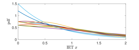
Figure 1: MoE IET densities.

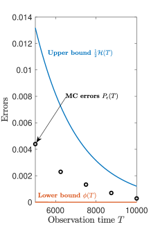
(a) Errors and bounds

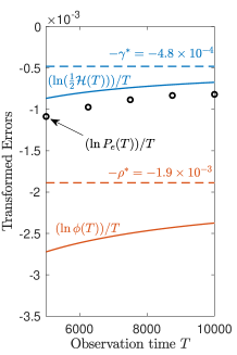
(b) Transformed errorsand bounds

Figure 2: MC error probabilities and error bounds: (a) For $T\geq 5000$, the error probabilities are bounded by the asymptotic bounds. (b) The transformed plots show that the error probability $P_{e}(T)$ has asymptotically exponential decay.

7 Conclusion

In this paper we studied, for the first time, the asymptotics of the multi-class misclassification error probability ($P_{e}(T))$ for point processes. After extending some standard entropy based analog bounds to point processes the analysis proceeded in four stages.

Firstly we extended recent pair-wise Bhattacharyya and Kullback-Liebler affinity based entropy bounds to the point process case. Secondly we develop a new asymptotic inverse Fano theorem that enables asymptotic calculation of both lower and upper bounds. Then thirdly, we specialised to the renewal processes case. We found the Laplace transforms of the Bhattacharyya affinity and the Kullback-Liebler divergence and thus derived asymptotic expressions for these affinities.

Then in the fourth stage we put all this together to derive asymptotic upper and lower bounds on the mis-classification error probability (a.k.a. error rate) for multi-class classification of renewal processes. We illustrated the theory with a non-trivial Gamma example. And further illustrated the results with a medium sized simulation using a mixture of Erlang distributions.

In future work, we will tackle asymptotics for heavy-tailed renewal processes and for Hawkes processes.

Appendix A. Proofs for Section 3

Here we prove Lemma 2 and Theorem 1. The proof of Lemma 2 relies on the following ‘opposite’ Jensen’s inequality.

Lemma 6. KL upper bound.
Consider the mixture density $p(x)={\textstyle\sum}_{k=1}^{M}\pi_{k}p_{k}(x)$ for an analog random variable and introduce $D_{kj}=D(p_{k}||p_{j})$, $K_{kj}=e^{-D_{kj}}$ as well as $D_{k}={\textstyle\sum}_{j=1}^{M}\pi_{j}K_{kj}$. Then,

$$D(p_{k}||p)\leq-\ln D_{k},$$

The proof is given after the proof of Lemma 2.

$\bullet$ Proof of Lemma 2.

(a) The MI lower bound is proved in [22],[14]. The MI upper bound is stated in [22],[14], but depends on a key lemma from [19], [28]. But [28] is not available and [19] does not have the key lemma. Thus, we give a new short direct proof of the upper bound using Lemma 6.

To finish the proof of (a) multiply through the inequality in Lemma 6 by $\pi_{k}$ and sum to obtain

$$\mathcal{I}(T) ={\textstyle\sum}_{k=1}^{M}\frac{\pi_{k}}{\ln 2}D(L_{k}||L)$$

$$\leq-{\textstyle\sum}_{k=1}^{M}\pi_{k}\log({\textstyle\sum}_{j=1}^{M}\pi_{j}K_{kj})=M_{K}.$$

(b) Use the information relation $\mathcal{H}(T)=\mathcal{H}(C)-\mathcal{I}(T)$ to get

$$\mathcal{H}(T) \leq\mathcal{H}(C)-M_{R}(T)$$

$$=-{\textstyle\sum}_{k=1}^{M}\pi_{k}\log\pi_{k}+{\textstyle\sum}_{k=1}^{M}\pi_{k}\log({\textstyle\sum}_{j=1}^{M}\pi_{j}R_{kj})$$

$$={\textstyle\sum}_{k=1}^{M}\pi_{k}\log\left[1+{\textstyle\sum}_{j\neq k}\frac{\pi_{j}}{\pi_{k}}R_{kj}(T)\right]=\mathcal{H}_{R}(T)$$

$$\mathcal{H}(T) \geq\mathcal{H}(C)-M_{R}(T)$$

$$=-{\textstyle\sum}_{k=1}^{M}\pi_{k}\log\pi_{k}+{\textstyle\sum}_{k=1}^{M}\pi_{k}\log({\textstyle\sum}_{j=1}^{M}\pi_{j}K_{kj})$$

$$={\textstyle\sum}_{k=1}^{M}\pi_{k}\log\left[1+{\textstyle\sum}_{j\neq k}\frac{\pi_{j}}{\pi_{k}}K_{kj}(T)\right]=\mathcal{H}_{K}(T).$$

(c) Applying Lemma 1 gives the result. $\square$

$\bullet$ Proof of Lemma 6.

Let $\omega_{j},j=1,\dotsm,M$ be a mass function to be chosen. Now with $k$ fixed, apply the log-sum inequality to find

$${\textstyle\sum}_{j}\left(\omega_{j}p_{k}(x)\ln\frac{\omega_{j}p_{k}(x)}{\pi_{j}p_{j}(x)}\right)\geq \left({\textstyle\sum}_{j}\omega_{j}p_{k}(x)\right)\ln\frac{{\textstyle\sum}_{j}\omega_{j}p_{k}(x)}{{\textstyle\sum}_{j}\pi_{j}p_{j}(x)}$$

$$= p_{k}(x)\ln\frac{p_{k}(x)}{p(x)}.$$

Integrate both sides to obtain

$$LHS ={\textstyle\sum}_{j}\omega_{j}\int p_{k}(x)\ln\frac{\omega_{j}p_{k}(x)}{\pi_{j}p_{j}(x)}dx\geq D(p_{k}||p).$$

We now rewrite the LHS as follows

$$LHS ={\textstyle\sum}_{j}\omega_{j}\ln\frac{\omega_{j}}{\pi_{j}}+{\textstyle\sum}_{j}\omega_{j}\int p_{k}(x)\ln\frac{p_{k}(x)}{p_{j}(x)}dx$$

$$={\textstyle\sum}_{j}\omega_{j}\ln\frac{\omega_{j}}{\pi_{j}}+{\textstyle\sum}_{j}\omega_{j}D_{kj}.$$

We choose $\omega_{j}$ to minimize the LHS. Adding a Lagrangian penalty $\lambda({\textstyle\sum}_{j}\omega_{j}-1)$ and differentiating w.r.t $\omega_{j}$ gives

$$\begin{array}[]{rrcl}&0&=&\ln\frac{\omega_{j}}{\pi_{j}}+1+D_{kj}+\lambda\\ \Rightarrow&\ln\frac{\omega_{j}}{\pi_{j}}&=&-(\lambda+1)-D_{kj}\\ \Rightarrow&\omega_{j}&=&C\pi_{j}e^{-D_{kj}}=C\pi_{j}K_{kj},\quad C=e^{-(\lambda+1)}.\end{array}$$

Applying the constraint ${\textstyle\sum}_{j}\omega_{j}=1$ gives $\omega_{j}=\frac{\pi_{j}K_{kj}}{D_{k}}.$

The minimized LHS is then

$$LHS ={\textstyle\sum}_{j}\omega_{j}\ln\frac{\omega_{j}}{\pi_{j}}+{\textstyle\sum}_{j}\omega_{j}D_{kj}$$

$$=\frac{1}{D_{k}}{\textstyle\sum}_{j}\pi_{j}K_{kj}\ln\frac{e^{-D_{kj}}}{D_{k}}+\frac{1}{D_{k}}{\textstyle\sum}_{j}D_{kj}\pi_{j}K_{kj}$$

$$=\frac{1}{D_{k}}{\textstyle\sum}_{j}\pi_{j}K_{kj}\left(-D_{kj}-\ln{D_{k}}\right)+\frac{1}{D_{k}}{\textstyle\sum}_{j}D_{kj}\pi_{j}K_{kj}$$

$$=-\ln D_{k}.$$

which gives the result.

$\bullet$ Proof of Theorem 1.

For convenience, we write $\mathcal{H}_{T}=(\ln 2)\mathcal{H}(T)$. $\mathcal{H}_{T}$ is positive and decreases to $0$. So we can write $\mathcal{H}_{T}=e^{-F_{T}}$, with $F_{T}\to\infty$. Then,

$$e^{F_{T}}\phi_{T}\ln\frac{1}{\phi_{T}}+e^{F_{T}}(1-\phi_{T})\ln\frac{1}{1-\phi_{T}}+de^{F_{T}}\phi_{T}=1.$$

Note that all three terms on the LHS are positive. So as $T\to\infty$ and $F_{T}\to\infty$ we must have $\phi_{T}\to 0$. So we can introduce

$$0\leq\rho_{T}=(1-\phi_{T})\phi_{T}e^{F_{T}}\leq e^{F_{T}}(1-\phi_{T})\ln\frac{1}{1-\phi_{T}}\leq 1,$$

since, for $0\leq\phi\leq 1$

$$\phi(1-\phi)\leq-(1-\phi)\ln(1-\phi)\leq\phi.$$ (7.1)

Then, multiply through the identity above to find:

$$\begin{array}[]{rrcl}&&&1-\phi_{T}\\ &&=&(1-\phi_{T})e^{F_{T}}\phi_{T}\ln\frac{1}{\phi_{T}}\\ &&&+e^{F_{T}}(1-\phi_{T})^{2}\ln\frac{1}{1-\phi_{T}}+d\phi_{T}(1-\phi_{T})e^{F_{T}}\\ &&=&\rho_{T}\ln\frac{(1-\phi_{T})e^{F_{T}}}{\phi_{T}(1-\phi_{T})e^{F_{T}}}+e^{F_{T}}(1-\phi_{T})^{2}\ln\frac{1}{1-\phi_{T}}+d\rho_{T}\\ &&=&\rho_{T}\ln\frac{1}{\rho_{T}}+(1-\phi_{T})\phi_{T}e^{F_{T}}\left(F_{T}-\ln\frac{1}{1-\phi_{T}}\right)\\ &&&+e^{F_{T}}(1-\phi_{T})^{2}\ln\frac{1}{1-\phi_{T}}+d\rho_{T}\\ &&=&\rho_{T}\ln\frac{1}{\rho_{T}}+F_{T}\rho_{T}\\ &&&+e^{F_{T}}(1-\phi_{T})(1-\phi_{T})\ln\frac{1}{1-\phi_{T}}+d\rho_{T}.\end{array}$$

Now all terms are $>0$ and $0<\rho_{T}\leq 1$. So letting $T\to\infty$ we get $F_{T}\to\infty$ and $1-\phi_{T}\rightarrow 1$ and so must have $\rho_{T}\to 0$.

Then, as $T\to\infty$, the first term $\rho_{T}\ln\frac{1}{\rho_{T}}\to 0$, the last term $d\rho_{T}\to 0$ and due to (7.1), the third term

$$e^{F_{T}}(1-\phi_{T})(1-\phi_{T})\ln\frac{1}{1-\phi_{T}} \leq e^{F_{T}}(1-\phi_{T})\phi_{T}=\rho_{T}\to 0.$$

So, we are left with, as $T\to\infty$,

$$F_{T}\rho_{T}=F_{T}e^{F_{T}}\phi_{T}(1-\phi_{T})\to 1$$

$$\Rightarrow F_{T}e^{F_{T}}\phi_{T}\to 1$$

$$\Rightarrow \phi_{T}\sim\frac{e^{-F_{T}}}{F_{T}}=\frac{\mathcal{H}_{T}}{-\log\mathcal{H}_{T}}.$$

$\square$

B. Proofs for Section 4

B.1. Proofs for Section 4 A.

Proof of Lemma 4. We have

$$D_{kj}(T) =\operatorname{E}_{k}\left[\ln\frac{L_{k}(N_{0}^{T})}{L_{j}(N_{0}^{T})}\right]$$

$$=\operatorname{E}_{k}\left[{\textstyle\sum}_{r=1}^{N_{T}}\ln\frac{\lambda_{k}(T_{r})}{\lambda_{j}(T_{r})}-\int_{0}^{T}\lambda_{k}(t)-\lambda_{j}(t)dt\right]$$

$$=\operatorname{E}_{k}\left[\int_{0}^{T}\ln\frac{\lambda_{k}(t)}{\lambda_{j}(t)}dN_{t}-\int_{0}^{T}\lambda_{k}(t)-\lambda_{j}(t)dt\right]$$

$$=\operatorname{E}_{k}\left[\int_{0}^{T}\lambda_{k}(t)\ln\frac{\lambda_{k}(t)}{\lambda_{j}(t)}-\lambda_{k}(t)+\lambda_{j}(t)dt\right]$$

$$=\int_{0}^{T}\operatorname{E}_{k}[\lambda_{k}(t)\lambda_{kj}(t)]dt,$$

where $\lambda_{kj}(t)=\frac{\lambda_{j}(t)}{\lambda_{k}(t)}-1-\ln\frac{\lambda_{j}(t)}{\lambda_{k}(t)}$.

We replaced the summation with the Lebesgue-Stieltjes integral of the counting measure in the third line. And we used the martingale property of $dN_{t}-\lambda(t)dt$ in the second last line ([10] and [4]).

Using the classic hazard relations in Section 2, we can rewrite the Janossy density

$$L_{k}(N_{0}^{T}) ={\textstyle\prod}_{r=1}^{n}\lambda_{k}(t_{r})e^{-\Lambda_{k}(T)}$$

$$={\textstyle\prod}_{r=1}^{n}p_{k}(t_{r}-t_{r-1})S_{k}(T-t_{n}),$$

with $t_{0}=0$. Further

$$\lambda_{k}(t)\lambda_{kj}(t) =h_{k}(t-t_{n})\left(\frac{h_{j}(t-t_{n})}{h_{k}(t-t_{n})}-1-\ln\frac{h_{j}(t-t_{n})}{h_{k}(t-t_{n})}\right)$$

$$\equiv h_{k}(t-t_{n})h_{kj}(t-t_{n}),$$

We note also that

$$B_{kj}(x) =p_{k}(x)h_{kj}(x)=q_{kj}(x)+\frac{dF_{kj}(x)}{dx}.$$

We now find $\operatorname{E}_{k}[\lambda_{k}(t)\lambda_{kj}(t)]={\textstyle\sum}_{0}^{\infty}\int{\cal J}_{n}dt_{1}^{n}$ where

$${\cal J}_{n} ={\textstyle\prod}_{r=1}^{n}p_{k}(t_{r}-t_{r-1})S_{k}(t-t_{n})h_{k}(t-t_{n})h_{kj}(t-t_{n})$$

$$={\textstyle\prod}_{r=1}^{n}p_{k}(t_{r}-t_{r-1})p_{k}(t-t_{n})h_{kj}(t-t_{n})$$

$$={\textstyle\prod}_{r=1}^{n}p_{k}(t_{r}-t_{r-1})B_{kj}(t-t_{n}).$$

We now integrate backwards from $t_{n}$, finding

$$\int_{t_{n-1}}^{t}{\textstyle\prod}_{r=1}^{n}p_{k}(t_{r}-t_{r-1})B_{kj}(t-t_{n})dt_{n}$$

$$= {\textstyle\prod}_{r=1}^{n-1}p_{k}(t_{r}-t_{r-1})\int_{0}^{t-t_{n-1}}p_{k}(x_{n})B_{kj}(t-t_{n-1}-x_{n})dx_{n}$$

$$= {\textstyle\prod}_{r=1}^{n-1}p_{k}(t_{r}-t_{r-1})(B_{kj}\star p_{k})(t-t_{n-1}),$$

where $(f*g)(t)=\int_{0}^{t}f(u)g(t-u)du$ is a convolution. Continuing the backwards integration gives

$$\begin{array}[]{rcll}&\operatorname{E}_{k}[\lambda_{k}(t)\lambda_{kj}(t)]&=&B_{kj}(t)+{\textstyle\sum}_{n=1}^{\infty}(B_{kj}\star p_{k}^{(n)})(t)\\ \Rightarrow&\bar{D}_{kj}(s)&=&\frac{1}{s}\left(\bar{B}_{kj}(s)+{\textstyle\sum}_{n=1}^{\infty}\bar{B}_{kj}(s)\bar{p}_{k}^{n}(s)\right)\\ &&=&\frac{\bar{B}_{kj}(s)}{s(1-\bar{p}_{k}(s))}.\end{array}$$

$\square$

B.2. Proofs for Section 4 B.

Now for Theorem 2, apparently we can get this result from one in [17]. But [17] does not give existence conditions for $\gamma_{kj}$ and the integrals in (a) and (b). We therefore take a different approach, based on the Blackwell’s final value theorem (FVT).

Lemma 6.

Blackwell’s Final Value Theorem [2]. Let $g(x)$ have LT $\bar{g}(s)=\frac{\bar{r}(s)}{1-\bar{p}(s)}$, where $\bar{p}(s)$ is the LT of a probability density $p(x)$. Then,

$$\lim_{s\to 0}s\bar{g}(s)=c\Rightarrow\lim_{x\to\infty}g(x)=c=\frac{1}{\mu}\bar{r}(0),$$

where $\mu=-\bar{p}^{\prime}(0)=\int_{0}^{\infty}up(u)du$.

Remark. The FVT in traditional engineering applications assumes the LT is rational. Lemma 6 is a deeper result, for non-rational LTs, needed for our theory below.

Proof of Theorem 2. We have to show $e^{\gamma_{kj}T}R_{kj}(T)\to\alpha_{kj}$ as $T\to\infty$. We use Blackwell’s FVT to do this. Since $\bar{R}_{kj}(s)=\frac{\bar{G}_{kj}(s)}{1-\bar{p}_{kj}(s)},$ then $e^{\gamma_{kj}T}R_{kj}(T)$ has LT

$$\bar{R}_{kj}(s-\gamma_{kj})=\frac{\bar{G}_{kj}(s-\gamma_{kj})}{1-\bar{p}_{kj}(s-\gamma_{kj})}.$$

To apply the FVT we need to check that $\bar{p}_{kj}(s-\gamma_{kj})$ is the LT of a probability density i.e. that $\bar{p}_{kj}(-\gamma_{kj})=1$. However this holds since $\bar{p}_{kj}(-\gamma_{kj})=\int_{0}^{\infty}e^{\gamma_{kj}x}p_{kj}(x)dx=\int_{0}^{\infty}p_{kj}^{*}(x)dx=1$.

The FVT now gives

$$\alpha_{kj} =\lim_{s\to 0}s\bar{R}_{kj}(s-\gamma_{kj})$$

$$=\lim_{s\to 0}\frac{\bar{G}_{kj}(s-\gamma_{kj})}{\frac{1}{s}(1-\bar{p}_{kj}(s-\gamma_{kj}))}$$

$$=\frac{\bar{G}_{kj}(-\gamma_{kj})}{-\bar{p}_{kj}^{\prime}(-\gamma_{kj})}$$

By the elementary inequality $2ab\leq a^{2}+b^{2}$ we find

$$\bar{p}_{kj}(0)<\int_{0}^{\infty}\frac{1}{2}(p_{k}(x)+p_{j}(x))dx=1.$$

By Definition 4, we can find a $\gamma_{kj}>0$ such that $\bar{p}_{kj}(-\gamma_{kj})<\infty$. Then, since $\bar{p}_{kj}(-\gamma)$ is a continuous and increasing function of $\gamma$ and $\bar{p}_{kj}(-\infty)=\infty$, we can find a unique $0<\gamma_{kj}<\infty$, such that $\bar{p}_{kj}(-\gamma_{kj})=1$. $\square$

$\bullet$ Proof of Lemma 5. With A1, we can find $x_{k}^{*},x_{j}^{*}$, such that $\inf_{x>x_{k}^{*}}h_{k}(x)=z_{k}>0$ and $\inf_{x>x_{j}^{*}}h_{j}(x)=z_{j}>0$. Suppose $\bar{G}_{kj}(-\gamma_{kj})=\infty$. Let $x^{*}=\max\{x_{k}^{*},x_{j}^{*}\}$. Then, use the classic hazard relations to find

$$\bar{p}_{kj}(-\gamma_{kj}) =g+\int_{x^{*}}^{\infty}\sqrt{h_{k}(x)h_{j}(x)}e^{\gamma_{kj}x}G_{kj}(x)dx$$

$$\geq g+\sqrt{z_{k}z_{j}}\int_{x^{*}}^{\infty}e^{\gamma_{kj}x}G_{kj}(x)dx=\infty,$$

where $g=\int_{0}^{x^{*}}p_{kj}^{*}(x)dx<\infty$. This contradicts $\bar{p}_{kj}(-\gamma_{kj})=1$ and the result follows. $\square$

$\bullet$ We are left with the discussion of condition (b): $\int_{0}^{\infty}xp_{kj}^{*}(x)dx<\infty$. First, suppose at least one of $p_{k}$ and $p_{j}$, say $p_{k}$, has $\int_{0}^{\infty}e^{\theta x}p_{k}(x)dx<\infty$ for all real $\theta$, e.g. $p_{k}(x)\sim e^{-x^{2}}$. Then, it is straightforward to show that condition (b) $\int_{0}^{\infty}xp_{kj}^{*}(x)dx=\int_{0}^{\infty}x\sqrt{p_{k}(x)p_{j}(x)}dx<\infty$ is always satisfied, since $p_{kj}^{*}$ is also regular and thus the first moment exists.

Now suppose there exist $\theta_{k}^{*},\theta_{j}^{*}>0$, such that the MGFs $m_{k}(\theta)=\int_{0}^{\infty}e^{\theta x}p_{k}(x)dx$ and $m_{j}(\theta)=\int_{0}^{\infty}e^{\theta x}p_{j}(x)dx$ exist for all $\theta<\theta_{k}^{*}$ and $\theta<\theta_{j}^{*}$, respectively. But $m_{k}(\theta)=\infty,m_{j}(\theta)=\infty$ for $\theta>\theta_{k}^{*}$ and $\theta>\theta_{j}^{*}$. Then we must have $\gamma_{kj}\leq\frac{\theta_{k}^{*}+\theta_{j}^{*}}{2}$.

For the case where $\gamma_{kj}<\frac{\theta_{k}^{*}+\theta_{j}^{*}}{2}$, clearly $p_{kj}^{*}$ is regular and thus condition (b) is satisfied. For the extreme case $\gamma_{kj}=\frac{\theta_{k}^{*}+\theta_{j}^{*}}{2}$, it is possible that the first moment does not exist. However, such a case has measure $0$.

B.3. Proofs for Section 4 C.

Proof of Theorem 3. Introduce $g(T)=D_{kj}(T)-\rho_{kj}T$. We need to show that as $s\to 0$, $s\bar{g}(s)\to\ln c_{kj}$. So that, by Blackwell’s FVT, as $T\to\infty$,

$$\begin{array}[]{rrl}&D_{kj}(T)-\rho_{kj}T&\to\ln c_{kj}\\ \equiv&e^{\rho_{kj}T}K_{kj}(T)=e^{\rho_{kj}T-D_{kj}(T)}&\to c_{kj}.\end{array}$$

So noting that $\bar{S}_{k}(s)=\frac{1-\bar{p}_{k}(s)}{s}$, we get

$$s\bar{g}(s) =s\bar{D}_{kj}(s)-\frac{\rho_{kj}}{s}$$

$$=\frac{\bar{B}_{kj}(s)}{1-\bar{p}_{k}(s)}-\frac{\rho_{kj}}{s}$$

$$=\frac{\frac{1}{s}(\bar{q}_{kj}(s)-\rho_{kj}\bar{S}_{k}(s))+\bar{F}_{kj}(s)}{\bar{S}_{k}(s)}.$$

We then have

$$\lim_{s\to 0}s\bar{g}(s)=\frac{\left[\lim_{s\to 0}\frac{1}{s}\bar{\chi}(s)\right]+\bar{F}_{kj}(0)}{\mu_{k}},$$

where $\bar{\chi}(s)=\bar{q}_{kj}(s)-\rho_{kj}\bar{S}_{k}(s)$ and (c) $\bar{F}_{kj}(0)=\int_{0}^{\infty}F_{kj}(x)dx<\infty$ is to be proved.

We have $\bar{\chi}(0)=\bar{q}_{kj}(0)-\frac{\bar{q}_{kj}(0)}{\mu_{k}}\mu_{k}=0.$ But the LT relations give

$$\lim_{s\to 0}\bar{\chi}^{\prime}(s) =-\int_{0}^{\infty}xq_{kj}(x)dx+\rho_{kj}\int_{0}^{\infty}xS_{k}(x)dx$$

$$=-\int_{0}^{\infty}xq_{kj}(x)dx+\frac{1}{2}\rho_{kj}\int_{0}^{\infty}x^{2}p_{k}(x)dx$$

$$=\bar{q}_{kj}^{\prime}(0)+\frac{1}{2}\rho_{kj}(\sigma_{k}^{2}+\mu_{k}^{2}),$$

where $-\bar{q}_{kj}^{\prime}(0)=\int_{0}^{\infty}xp_{k}(x)\ln\frac{p_{k}(x)}{p_{j}(x)}dx<\infty$ by A2*, and $\sigma_{k}^{2}=\operatorname{var}_{k}[X]<\infty$ is ensured by existence of the MGF.

So, by L’Hopital’s rule,

$$\begin{array}[]{rrcl}&\lim_{s\to 0}\frac{1}{s}\chi(s)&=&\bar{q}_{kj}^{\prime}(0)+\frac{1}{2}\rho_{kj}(\sigma_{k}^{2}+\mu_{k}^{2})\\ \Rightarrow&\lim_{s\to 0}s\bar{g}(s)&=&\ln c_{kj},\end{array}$$

as required. $\square$

We now prove that condition (c) holds under A2*.

Lemma 7.

Log-integral Tail Lemma. Let $p_{k}(x),p_{j}(x)$ be densities with survivors $S_{k}(x),S_{j}(x)$. Then

$$\int_{x}^{\infty}p_{k}(u)\ln\frac{p_{k}(u)}{p_{j}(u)}du\geq S_{k}(x)\ln\frac{S_{k}(x)}{S_{j}(x)}.$$

Further,

$$\int_{0}^{\infty}up_{k}(u)\ln\frac{p_{k}(u)}{p_{j}(u)}du\geq\int_{0}^{\infty}S_{k}(x)\ln\frac{S_{k}(x)}{S_{j}(x)}dx.$$

Proof.

Let $f,g,F,G$ be positive numbers. In the inequality $x\ln x-x+1\geq 0,x\geq 0,$ set $x=\frac{f/F}{g/G}$. Then,

$$\begin{array}[]{rrcl}&0&\leq&\frac{f/F}{g/G}\ln\frac{f/F}{g/G}-\frac{f/F}{g/G}+1\\ \Rightarrow&0&\leq&\frac{f}{F}\ln\frac{f/F}{g/G}-\frac{f}{F}+\frac{g}{G}\\ \Rightarrow&0&\leq&\frac{f}{F}\ln\frac{f}{F}-\frac{f}{F}\ln\frac{g}{G}-\frac{f}{F}+\frac{g}{G}.\end{array}$$

Now set $f=p_{k}(u),g=p_{j}(u),F=S_{k}(u),G=S_{j}(u)$ and integrate $u$ from $x$ to $\infty$ to find

$$\frac{1}{S_{k}(x)}\int_{x}^{\infty}p_{k}(u)\ln\frac{p_{k}(u)}{p_{j}(u)}du-\ln\frac{S_{k}(u)}{S_{j}(u)}\geq 0,$$

which delivers the first result.

Then, integrating through the first inequality gives

$$\int_{0}^{\infty}\int_{x}^{\infty}p_{k}(u)\ln\frac{p_{k}(u)}{p_{j}(u)}dudx\geq\int_{0}^{\infty}S_{k}(x)\ln\frac{S_{k}(x)}{S_{j}(x)}dx.$$

Changing the order of integration on the left-hand side gives the quoted second result. Thus A2* $\Rightarrow$ (c).∎

C. Proofs for Section 5

Proof of Theorem 4. The first two parts are just the results in Theorem 2 and 3. By the equivalence $\log(1+f)\sim\frac{1}{\ln 2}f$ as $f\to 0$, we have

$$(\ln 2)\mathcal{H}_{R}(T) \sim{\textstyle\sum}_{k=1}^{M}{\textstyle\sum}_{j\neq k}\pi_{j}R_{kj}(T)\sim\alpha^{*}e^{-\gamma^{*}T}$$

$$(\ln 2)\mathcal{H}_{K}(T) \sim{\textstyle\sum}_{k=1}^{M}{\textstyle\sum}_{j\neq k}\pi_{j}K_{kj}(T)\sim c^{*}e^{-\rho^{*}T},$$

where $\alpha^{*}e^{-\gamma^{*}T}$ and $c^{*}e^{-\rho^{*}T}$ are the most slowly decaying terms among $R_{kj}(T)$ and $K_{kj}(T)$, respectively.

The quoted bounds are from Lemma 2(c). For the upper bound,

$$\frac{1}{2}\mathcal{H}_{R}(T)\sim\frac{1}{2\ln 2}\alpha^{*}e^{-\gamma^{*}T}.$$

For the lower bound, we have $K_{kj}(T)\sim c_{kj}e^{-\rho_{kj}T}\to 0$ as $T\to\infty$. Then obviously $\mathcal{H}_{K}(T)\to 0$. We then apply Theorem 1 to find

$$\phi_{T}\sim\frac{{\cal H}_{K}(T)}{-\log{\cal H}_{K}(T)}\sim\frac{\frac{c^{*}}{\ln 2}e^{-\rho^{*}T}}{\frac{\rho^{*}}{\ln 2}T}=\frac{c^{*}}{\rho^{*}}\frac{1}{T}e^{-\rho^{*}T}.$$

$\square$

References

• [1] William Bialek, Rob de Ruyter van Steveninck, Fred Rieke, and David Warland. Spikes: Exploring the Neural Code. MIT press, 1997.
• [2] N.H. Bingham, C.M. Goldie, and J.L. Teugels. Regular Variation. Encyclopedia of Mathematics and its Applications. Cambridge University Press, Cambridge, U.K., 1987.
• [3] R. Blahut. Hypothesis testing and information theory. IEEE Transactions on Information Theory, 20(4):405–417, 1974.
• [4] Pierre Brémaud. Point Process Calculus in Time and Space, volume 98 of Probability Theory and Stochastic Modelling. Springer, Cham, Switzerland, 1 edition, 2020.
• [5] Lisbeth Carstensen, Albin Sandelin, Ole Winther, and Niels R. Hansen. Multivariate hawkes process models of the occurrence of regulatory elements. BMC Bioinformatics, 11(1):456, 2010.
• [6] C. H. Chen. On information and distance measures, error bounds, and feature selection. Information Sciences, 10(2):159–173, 1976.
• [7] Herman Chernoff. A measure of asymptotic efficiency for tests of a hypothesis based on the sum of observations. The Annals of Mathematical Statistics, 23(4):493–507, 15, 1952.
• [8] Thomas M. Cover and Joy A. Thomas. Elements of Information Theory. John Wiley Sons, New York, 1991.
• [9] Jr. D. P. Gaver. Observing stochastic processes, and approximate transform inversion. Operations Research, 14(3):444–459, 1966.
• [10] D. Daley and D Vere-Jones. An introduction to the theory of point processes. 1, 2003.
• [11] L. Davisson, G. Longo, and A. Sgarro. The error exponent for the noiseless encoding of finite ergodic markov sources. IEEE Transactions on Information Theory, 27(4):431–438, 1981.
• [12] Luc Devroye. Non-Uniform Random Variate Generation. Springer-Verlag, New York, 1986.
• [13] Luc Devroye, Laszlo Gyorfi, and Gabor Lugosi. A Probabilistic Theory of Pattern Recognition. New York : Springer, New York, 1996.
• [14] Yijun Ding and Amit Ashok. Bounds on mutual information of mixture data for classification tasks. Journal of the Optical Society of America A, 39(7):1160–1171, 2022.
• [15] H Dubner and J Abate. Numerical inversion of laplace transforms by relating them to the finite fourier cosine transform. J. ACM, 15:115–123, 1968.
• [16] Richard O. Duda, Peter E. Hart, and David G. Stork. Pattern Classification. Wiley, New York, 2 edition, 2001.
• [17] William Feller. An Introduction to Probability Theory and its Applications, volume 2. John Wiley Sons, New York, 2 edition, 1991.
• [18] M. Gutman. Asymptotically optimal classification for multiple tests with empirically observed statistics. IEEE Transactions on Information Theory, 35(2):401–408, 1989.
• [19] J. R. Hershey and P. A. Olsen. Approximating the kullback leibler divergence between gaussian mixture models. In IEEE International Conference on Acoustics, Speech and Signal Processing, volume 4, pages IV–317–IV–320, 2007.
• [20] Gábor Horváth, Illés Horváth, Salah Al-Deen Almousa, and Miklós Telek. Numerical inverse laplace transformation using concentrated matrix exponential distributions. Performance Evaluation, 137:102067, 2020.
• [21] T. Kailath. The divergence and bhattacharyya distance measures in signal selection. IEEE Transactions on Communication Technology, 15(1):52–60, 1967.
• [22] Artemy Kolchinsky and Brendan D. Tracey. Estimating mixture entropy with pairwise distances. Entropy, 19(7):361, 2017.
• [23] V. A. Kovalevskij. The Problem of Character Recognition from the Point of View of Mathematical Statistics. Spartan, New York, 1968.
• [24] P. A. W Lewis and G. S. Shedler. Simulation of nonhomogeneous poisson processes by thinning. Naval Research Logistics Quarterly, 26(3):403–413, 1979.
• [25] Jianhua Lin. Divergence measures based on the shannon entropy. IEEE Transactions on Information Theory, 37:145–151, 1991.
• [26] Michal Lukasik, P. K. Srijith, Duy Vu, Kalina Bontcheva, Arkaitz Zubiaga, and Trevor Cohn. Hawkes processes for continuous time sequence classification: an application to rumour stance classification in twitter. Proc. 54th Annual Meeting of ACL, pages 393–398. Ass. Comp. Linguistics, 2016.
• [27] Y. Ogata. On lewis’ simulation method for point processes. IEEE Transactions on Information Theory, 27(1):23–31, 1981.
• [28] J. Paisley. Two useful bounds for variational inference. Report, Princeton University, 2010.
• [29] Mirosław Pawlak, Mateusz Pabian, and Dominik Rzepka. Asymptotically optimal nonparametric classification rules for spike train data. In IEEE International Conference on Acoustics, Speech and Signal Processing, pages 1–5, 2023.
• [30] Mirosław Pawlak, Mateusz Pabian, and Dominik Rzepka. Bayes risk consistency of nonparametric classification rules for spike trains data, 2023.
• [31] S. Prasad. Bayesian error-based sequences of statistical information bounds. IEEE Transactions on Information Theory, 61(9):5052–5062, 2015.
• [32] X. Rong and V. Solo. On the error rate for classifying point processes. In IEEE Conference on Decision and Control, pages 120–125, 2021.
• [33] Frederic Schoenberg and Katherine Tranbarger. Description of earthquake aftershock sequences using prototype point patterns. Environmetrics, 19:271–286, 2008.
• [34] Salimeh Yasaei Sekeh, Brandon Oselio, and Alfred O. Hero. Learning to bound the multi-class bayes error. IEEE Transactions on Signal Processing, 68:3793–3807, 2020.
• [35] Dawei Shi, Ling Shi, and Tongwen Chen. Event-Based State Estimation: A Stochastic Perspective. Studies in Systems, Decision and Control. Springer, New York, 2016.
• [36] Harald Stehfest. Algorithm 368: Numerical inversion of laplace transforms. Commun. ACM, 13(1):47–49, 1970.
• [37] A. Talbot. The accurate numerical inversion of laplace transforms. IMA Journal of Applied Mathematics, 23(1):97–120, 1979.
• [38] J. Unnikrishnan and D. Huang. Weak convergence analysis of asymptotically optimal hypothesis tests. IEEE Transactions on Information Theory, 62(7):4285–4299, 2016.
• [39] JD. Victor and KP. Purpura. Metric-space analysis of spike trains: Theory, algorithms and application. Network: Computation in Neural Systems, 8(2):127–164, 1997.
• [40] A. Wisler, V. Berisha, D. Wei, K. Ramamurthy, and A. Spanias. Empirically-estimable multi-class classification bounds. In IEEE International Conference on Acoustics, Speech and Signal Processing, pages 2594–2598, 2016.
• [41] Sai Xiao, Athanasios Kottas, Bruno Sansó, and Hyotae Kim. Nonparametric bayesian modeling and estimation for renewal processes. Technometrics, 63:1–27, 2019.
• [42] Ke Zhou, Hongyuan Zha, and Le Song. Learning social infectivity in sparse low-rank networks using multi-dimensional hawkes processes. Journal of Machine Learning Research, 31:641–649, 2013.