Freezing and BPS jumping

Abstract

We report a novel BPS jumping phenomenon of 5d $\mathcal{N}=1$ supersymmetric gauge theories whose brane configuration is equipped with an O$7$-plane. The study of the relation between O$7{}^{+}$-plane and O$7{}^{-}$-plane reveals that such BPS jumps take place when the Higgsing is triggered near the O7-plane upon a particular parameter tuning of the theories. We propose two types of gauge theories whose BPS spectra jump. One is the SU($2N+8$) gauge theory with a symmetric hypermultiplet converted to the SU($2N$) gauge theory with an antisymmetric hypermultiplet. The other is pure SO($2N+8$) gauge theory jumping to pure Sp($N$) gauge theory. We explicitly confirm our proposal through the (un)refined instanton partition functions. Furthermore, we discuss feasible generalizations involving an O$p$-plane for supersymmetric gauge theories of eight supercharges in four and three dimensions ($p=6,5$ respectively).

1 Introduction

The study of supersymmetric gauge theories in string theory has undergone significant progress with the introduction and understanding of D-branes and orientifold planes (O-planes). D-branes, or Dirichlet-branes, are solitonic extended objects in string theory that open strings can end Polchinski:1995mt . Therefore, the stacking of multiple D-branes is instrumental in manifesting non-abelian gauge symmetries, which are indispensable in the formulation of gauge theories. Furthermore, D-branes preserve a fraction of the supersymmetry present in string theory setups. Consequently, they offer a framework for the realization of supersymmetric gauge theories, enhancing our understanding of the dynamics and dualities inherent in these theories.

In addition to D-branes, O-planes – fixed planes where strings reflect and alter their orientation Dai:1989ua – play a vital role in the construction of models with specific gauge groups. They enable the realization of orthogonal and symplectic gauge groups within string theory frameworks. O-planes are also crucial for canceling the net charge and tension introduced by D-branes, ensuring the consistency and stability of the theory.

The manipulation of brane configurations with O-planes enables the exploration of incredibly rich families of supersymmetric theories. This approach provides a geometrically simple and intuitively clear perspective on these theories. Moreover, the dynamics of branes, encompassing their movement and interaction, yields profound insights into the strongly coupled dynamics of supersymmetric gauge theories. Notable phenomena like the Hanany-Witten (HW) transition, which involves brane creation and annihilation Hanany:1996ie , and Sen’s decomposition of an O7^--plane into a pair of two 7-branes Sen:1996vd , exemplify the significance of novel brane dynamics. Utilizing the configuration and dynamics of D-branes with O-planes has repeatedly proven crucial in constructing and studying supersymmetric theories, leading to a deeper understanding of essential aspects like the moduli space of vacua, partition functions, and duality.

In this paper, we study $(p-2)$-dimensional supersymmetric gauge theories with eight supercharges constructed from D$(p-2)$-branes with an O$p^{\pm}$-plane. The setups give rise to not only Sp($N$)/SO($N$) gauge theories as mentioned, but also SU($N$) gauge theories with (anti-)symmetric hypermultiplet Landsteiner:1997ei ; Elitzur:1998ju ; Giveon:1998sr ; Bergman:2015dpa . Our investigation focuses on the idea of freezing: by adjusting the positions of $2^{p-4}$ D$p$-branes around an O$p^{-}$-plane, the effect is closely related to an O$p^{+}$-plane within Type II theory. Schematically, we write the freezing as

$$\mathrm{O}p^{+}~{}\sim~{}\mathrm{O}p^{-}+2^{p-4}~{}\textrm{D}p\Big{|}_{\textrm{fixed near O$p^{-}$}}~{}.$$ (1)

In fact, the case of $p=7$ was recently explored in Hayashi:2023boy ; Kim:2023qwh where the effects of an O7⁺-plane can be approximated by “freezing” eight D7-branes with an O7^--plane (O7${}^{-}+$8D7) in Type IIB brane configurations. This process involves adjustments to the mass parameters or chemical potentials associated with the global symmetries of the D7-branes in some observables. In fact, it has been tested in the context of Seiberg-Witten curves Hayashi:2023boy and is extendable to the level of partition functions Kim:2023qwh . This technique provides a useful method for calculating some partition functions for theories formulated with an O7⁺-plane, and moreover reveals non-trivial relationships between two theories. We delve into the freezing process by examining exact partition functions, with a focus on instanton partition functions Nekrasov:2002qd .

We must emphasize that the freezing method is not universally applicable to all physical observables nor does it imply a duality between theories. It is primarily effective for specific observables, such as the prepotential or instanton partition functions, where it offers an efficient computational strategy. While it does establish identities for certain observables, there exist observables that distinguish between the two configurations. Nevertheless, the freezing method unveils curious links between seemingly distinct theories, which deserve more investigation.

Subsequently, our analysis extends to the unfreezing process. During the freezing phase, $2^{p-4}$ D$p$-branes are utilized, but these can be removed by adjusting the positions of the “color” D$(p-2)$-branes and possibly adding more D$p$-branes near the O$p^{-}$-plane. This rearrangement is achieved through Hanany-Witten transitions Hanany:1996ie following the Higgsing of the D$(p-2)$-branes. This process provides yet another non-trivial relationship between two different configurations with an O$p^{\pm}$-plane. Remarkably, we find that instanton partition functions exhibit notable discontinuities during the process of unfreezing. Since the instanton partition functions are Witten indices counting half-BPS states of instantons, this indicates a novel BPS jumping phenomenon. This is rooted in a basic principle from elementary calculus class: integration and limit operations generally do not commute, schematically represented by

$$\int\lim\mathcal{Z}\neq\lim\int\mathcal{Z}~{}.$$ (2)

The instanton partition functions are evaluated by Jeffrey-Kirwan (JK) residue integrals jeffrey1995localization . Upon the specialization of parameters within the considered theory, these integrals encounter degenerate poles brion1999arrangement ; szenes2003toric ; Benini:2013xpa . As a result, the accurate computation of residues, following this parameter specialization, differs from a naive parameter substitution in the generic integrated expressions. This gives rise to the novel BPS jumping phenomenon. It is noteworthy that this phenomenon is different from wall-crossing phenomena Seiberg:1994rs as it occurs at special points in the parameter (moduli) space of the theory where new degenerate poles emerge in JK residue integrals. This phenomenon is indeed ubiquitous when we tune chemical potentials or fugacities in JK residue integrals. Thus, this phenomenon offers a new perspective for understanding and analyzing not only instanton partition functions but also a wider range of partition functions involving JK residue methods.

In our detailed analysis, we aim to elucidate how the unfreezing processes relate two instanton partition functions with multiplicity coefficients, as recently found in Nawata:2021dlk ; Chen:2023smd . In the context of 5-brane web configurations, D1-branes generate instantons in 5d theories so that this implies that D1-branes contribute distinct non-perturbative effects at certain configurations specifically associated with unfreezing. In other words, the configuration of branes during unfreezing leads to the creation/annihilation of unique instanton states, deviating from those observed at generic points in the parameter space. Moreover, the Witten index on the moduli spaces of instantons undergoes notable changes at particular chemical potential values, highlighting the novel dynamic nature across the parameter space.

The paper is outlined as follows. Central to our study, section 2 delves into the freezing and unfreezing process involving O7^±-plane in the 5-brane webs. As a warm-up, we review 5-brane web realization of 5d $\mathcal{N}=1$ supersymmetric gauge theories in Type IIB theory, and we proceed to examine the effects of the freezing and unfreezing from the lens of the cubic prepotentials. Our investigation then extends to the investigation of the (un)freezing process in terms of 5d instanton partition functions. Concretely, using the ADHM descriptions of instanton moduli spaces, we explicitly show non-trivial identities among instanton partition functions as direct outcomes of freezing and unfreezing. As an illuminating example of the identities, we deal with the relation of partition functions of E-string and M-string theory. It also elucidates the method for calculating E-string and M-string partition functions using 5d instanton partition functions. Finally, we explore the novel BPS jumping phenomenon during the unfreezing process using unrefined instanton partition functions.

Subsequently, we study the freezing and unfreezing processes in 4d and 3d theories with eight supercharges. As emphasized before, the freezing process does not lead to the identities of all the physical observables. In the realm of 4d $\mathcal{N}=2$ superconformal field theories, the superconformal index serves to differentiate between two theories related by the (un)freezing process with O6^±-plane. However, this process does reveal non-trivial connections among Schur indices. Similarly, in 3d $\mathcal{N}=4$ theories, both the superconformal and twisted indices can distinguish theories related by the (un)freezing process involving an O5^±-plane, yet they also show noteworthy identities between 3-sphere partition functions. These aspects are examined in section 3.

Several appendices supplement the main text. Appendix A fixes the notations and conventions employed throughout the paper. Appendix B details the contributions to ADHM integrals from various gauge and matter multiplets for instanton partition functions. Appendix C delves into the detailed computations of Jeffrey-Kirwan residues for instanton partition functions, with a particular emphasis on handling degenerate poles. Through detailed calculations of JK residues, we clarify the occurrence of BPS jumping due to the appearance of degenerate poles during the unfreezing process.

2 Freezing, unfreezing, and BPS jumping in 5d theories

2.1 5d cubic prepotential and freezing

To start, we review the freezing at the level of the cubic prepotential, discussed in Hayashi:2023boy , and propose yet another novel relation between theories involving an O7-plane in their brane configurations.

The cubic prepotential $\mathcal{F}$ governing Coulomb branch of 5d supersymmetric field theory of gauge group $G$ is given by Seiberg:1996bd ; Morrison:1996xf ; Intriligator:1997pq

$$\mathcal{F}(\phi)=\frac{1}{2g_{0}^{2}}h_{ij}\phi_{i}\phi_{j}+\frac{\kappa}{6}d_{ijk}\phi_{i}\phi_{j}\phi_{k}+\frac{1}{12}\bigg{(}\sum_{r\in\Delta}\left|r\cdot\phi\right|^{3}-\sum_{f}\sum_{w\in R_{f}}\left|w\cdot\phi+m_{f}\right|^{3}\bigg{)},$$ (3)

where $g_{0}$ is the gauge coupling, $h_{ij}=\mathrm{Tr}(T_{i}T_{j})$ with $T_{i}$ being the Cartan generators of Lie algebra $\mathfrak{g}$ associated with $G$, and $\phi$ is the vacuum expectation value of the scalar field in the vector multiplet. The one-loop contribution of the cubic prepotential is given in the last term where $\Delta$ is the root system of Lie algebra $\mathfrak{g}$, $w$ is the weight of a representation $R_{f}$, and $m_{f}$ are mass parameters for hypermultiplet in $R_{f}$. We note that the term with the coefficient $\frac{\kappa}{6}$ in (3) only exists for gauge group $G=\mathrm{SU}(N\geq 3)$ where $\kappa$ is the Chern-Simons (CS) level and $d_{ijk}=\frac{1}{2}\mathrm{Tr}(T_{i}\{T_{j},T_{k}\})$. If the cubic Casimir of the matter representation is odd, there is a parity anomaly that can be canceled by a CS term with a half-odd-integer level $\kappa$. In particular, in the case of $\operatorname{SU}(2N+1)$ gauge theory with (anti-)symmetric matter, a parity anomaly is present, requiring the introduction of a CS term with a half-odd-integer level.

We also remark that the 5d $\operatorname{Sp}(N)$ gauge theory has a discrete $\theta$-angle due to the fact that $\pi_{4}(\operatorname{Sp}(N))=\mathbb{Z}_{2}$ Morrison:1996xf ; Douglas:1996xp ; Bergman:2013ala . The $\theta$-angle crucially distinguishes the spectrum of the theory at the instanton level. In other words, $\operatorname{Sp}(N)_{\theta=0}$ gauge theory and $\operatorname{Sp}(N)_{\theta=\pi}$ gauge theory have distinct instanton partition functions, which will be discussed in detail in the following sections. On the other hand, as the cubic prepotential (3) is one-loop exact, the prepotential is insensitive to the discrete $\theta$ angle. For this reason, we do not introduce the discrete $\theta$-angle when writing a prepotential $\mathcal{F}(\phi)$. Moreover, for Sp($N$) gauge theory with fundamental hypermultiplets, the discrete $\theta$-angle difference can be understood from the sign difference of the fundamental hypermultiplet mass and so we omit the discrete $\theta$ angle in the presence of fundamental hypermultiplet for Sp($N$) gauge theory.

For convenience, we express the cubic prepotential in terms of the Coulomb branch parameters $a_{i}$, by setting all the masses of hypermultiplets to zero. For $G=\textrm{SU}(N)$, in the Weyl chamber $a_{1}\geq a_{2}\geq\cdots\geq a_{N-1}\geq 0$ and $a_{N}=-\sum_{i=1}^{N-1}a_{i}$, the cubic prepotential for $\mathrm{SU}(N)$ gauge theory at the CS level $\kappa$ with hypermultiplets in $N_{f}$ fundamental representations, $N_{a}$ antisymmetric representations, and $N_{s}$ symmetric representations (for short, $\mathrm{SU}(N)_{\kappa}+N_{f}\mathbf{F}+N_{a}\textbf{AS}+N_{s}\textbf{Sym}$) takes the form

$$\mathcal{F}_{\mathrm{SU}(N)_{\kappa}+N_{f}\mathbf{F}+N_{a}\textbf{AS}+N_{s}\textbf{Sym}}= ~{}\frac{1}{2g_{0}^{2}}\sum_{i=1}^{N}a_{i}^{2}+\frac{\kappa}{6}\sum_{i=1}^{N}a_{i}^{3}+\frac{1}{6}\sum_{i<j}^{N}(a_{i}-a_{j})^{3}$$ (4)

$$-\frac{N_{f}}{12}\sum_{i=1}^{N}|a_{i}|^{3}-\frac{N_{a}}{12}\sum_{i<j}^{N}|a_{i}+a_{j}|^{3}$$

$$-\frac{N_{s}}{12}\Big{(}\sum_{i=1}^{N}|2a_{i}|^{3}+\sum_{i<j}^{N}|a_{i}+a_{j}|^{3}\Big{)}\ .$$

For $G=\textrm{Sp}(N)$, in the Weyl chamber $a_{1}\geq a_{2}\geq\cdots\geq a_{N}\geq 0$, the cubic prepotential takes the form

$$\mathcal{F}_{\mathrm{Sp}(N)+N_{f}\mathbf{F}}=\frac{1}{g_{0}^{2}}\sum_{i=1}^{N}a_{i}^{2}+\frac{1}{6}\bigg{(}\!\sum_{i<j}^{N}\big{(}(a_{i}\!-\!a_{j})^{3}+(a_{i}\!+\!a_{j})^{3}\big{)}+(8\!-\!N_{f})\!\sum_{i=1}^{N}a_{i}^{3}\bigg{)}\ .$$ (5)

For $G=\textrm{SO}(2N)$, in the Weyl chamber $a_{1}\geq a_{2}\geq\cdots\geq a_{N}\geq 0$, the cubic prepotential takes the form

$$\mathcal{F}_{\mathrm{SO}(2N)+N_{f}\mathbf{F}}=\frac{1}{g_{0}^{2}}\sum_{i=1}^{N}a_{i}^{2}+\frac{1}{6}\bigg{(}\sum_{i<j}^{N}\big{(}(a_{i}-a_{j})^{3}+(a_{i}+a_{j})^{3}\big{)}-N_{f}\sum_{i=1}^{N}a_{i}^{3}\bigg{)}\ .$$ (6)

We note that it is well-known that $\operatorname{SU}(2N)$ gauge theory with an antisymmetric hypermultiplet or a symmetric hypermultiplet has a Higgs branch to $\operatorname{Sp}(N)$ or $\operatorname{SO}(2N)$, respectively,

$$\mathrm{SU}(2N)_{\kappa}+1\textbf{AS}~{} \xrightarrow{\text{Higgsing}}~{}\mathrm{Sp}(N)\ ,$$ (7)

$$\mathrm{SU}(2N)_{\kappa}+1\textbf{Sym}~{} \xrightarrow{\text{Higgsing}}~{}\mathrm{SO}(2N)\ ,$$ (8)

which can be seen from the cubic prepotential by setting $a_{2N+1-i}=-a_{i}$ as well as masses of the hypermultiplets to zero, $m_{\bf AS/Sym}=0$.

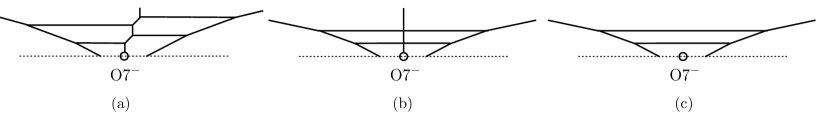
Figure 1: A Higgsing from SU($2N)+1\textbf{AS}$ to Sp($N$). As an example, we choose $N=2$. (a) a 5-brane web for SU($4)+1\textbf{AS}$. (b) The Coulomb branch parameters and the mass of an antisymmetric hypermultiplet are tuned so that the middle NS5-brane can be Higgsed. (c) The resulting 5-brane configuration after Higgsing the middle NS5-brane, which is a 5-brane web for Sp($2$).

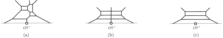
Figure 2: A Higgsing from SU($2N)+1\textbf{Sym}$ to SO($2N$). As an example, we choose $N=3$. (a) a 5-brane web for SU($6)+1\textbf{Sym}$. (b) The Coulomb branch parameters and the mass of a symmetric hypermultiplet are tuned so that the middle NS5-brane can be Higgsed. (c) The resulting 5-brane configuration after Higgsing the middle NS5-brane, which is a 5-brane web for SO($6$).

This Higgsing can be readily seen from 5-brane webs in Type IIB theory. Our convention for 5-brane webs is as follows: D5- and NS5-branes are extended in the $x^{0,1,2,3,4,6}$-directions and the $x^{0,1,2,3,4,5}$-directions, respectively so that their 5-brane configurations are constructed in the $x^{5,6}$-plane, called the $(p,q)$-plane. The fundamental hypermultiplets can be described by D7-branes which are extended in the $x^{0,1,2,3,4,7,8,9}$-directions so that a 7-brane in the $(p,q)$-plane appears as a dot on which 5-branes end. See Aharony:1997bh ; Hayashi:2018lyv for more details and examples.

Along with this convention, 5d $\operatorname{SU}(N)$ gauge theory with one (anti-)symmetric hypermultiplet is constructed by introducing an O7-plane on 5-brane web where a half NS5-brane is stuck Bergman:2015dpa . An O7^--plane gives rise to an antisymmetric hypermultiplet (e.g., see figure 1), while an O7⁺-plane gives rise to a symmetric hypermultiplet (e.g., see figure 2). The asymptotic horizontal distance of this middle NS5-brane from the position of an O7-plane is given by $\frac{N}{2}m_{\bf AS/Sym}$, a half of the mass of (anti-)symmetric hypermultiplet multiplied by the number of color branes Hayashi:2023boy . As an illustrative example, in figure 2(a), we present a 5-brane web for $\operatorname{SU}(6)+1\mathbf{Sym}$, where the fundamental region is given. One can imagine the covering space such that the projected image due to an O7⁺-plane is included below the monodromy cut of an O7⁺-plane (the dotted line in figure 2). To perform the Higgsing (7), the color D5-branes are aligned to realize the above Higgsing condition so that the middle NS5-brane is aligned, which is depicted in figure 2(b). The Higgsing takes place as follows. The parallel color D5-branes on the left and the right are reconnected and the middle half N5-brane brane is also connected through its reflected image so that the NS5-brane is taken away along the transverse directions where an O7-plane is extended. The resulting web is given in figure 2(c), which is a 5-brane web for pure $\operatorname{SO}(6)$, as expected.

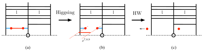
Figure 3: A Higgsing with a symmetric or antisymmetric hypermultiplet: $\operatorname{SU}(n)+1\textbf{AS}/\textbf{Sym}+N_{f}\mathbf{F}\to\operatorname{SU}(n-1)+1\textbf{AS}/\textbf{Sym}+(N_{f}-1)\mathbf{F}.$

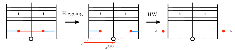
Figure 4: A Higgsing with a symmetric or an antisymmetric hypermultiplet reducing the Coulomb branch dimension by two: $\operatorname{SU}(n)+1\textbf{AS}/\textbf{Sym}+N_{f}\mathbf{F}\to\operatorname{SU}(n-2)+1\textbf{AS}/\textbf{Sym}+(N_{f}-2)\mathbf{F}.$

When there are additional $N_{f}$ fundamental hypermultiplets, there is another Higgs branch associated with fundamental hypermultiplets, which reduces the Coulomb branch dimension and the number of fundamental hypermultiplets by one:

$$\textrm{SU}(n)+1\textbf{AS}/\textbf{Sym}+N_{f}\mathbf{F}~{}\to~{}\operatorname{SU}(n-1)+1\textbf{AS}/\textbf{Sym}+(N_{f}-1)\mathbf{F}\ .$$ (9)

The corresponding 5-brane configuration is depicted in figure 3, where the brane charges are neglected to highlight the relevant Higgsing procedures. In figure 3(a), two (flavor) D7-branes, appearing red dots, are aligned on a color D5-brane in a way that recombination can take place such that the D5-brane in red ends on two D7-branes, while the D5-branes in blue are connected to a D7-brane and a 5-brane with NS5-charge in the middle. Once this recombination happens, as illustrated in figure 3(b), the D5-brane in red is Higgsed away along the transverse direction to 5-brane, which is denoted by the $x^{7,8,9}$-directions. Finally, one can take the Hanany-Witten (HW) transition so that a D7-brane on the left of figure 3(c) is decoupled becoming a free hypermultiplet, while a D7-brane on the right contributes to a fundamental hypermultiplet. As a result, this Higgsing described through the 5-brane web reduces the rank of the Coulomb branch and the flavor group by one, respectively. It is worth noting that this Higgsing takes out one fundamental hypermultiplet, to realize the Higgsing, one needs to tune masses of two fundamental hypermultiplets.

We note that the 5-brane configuration suggests another Higgsing process:

$$\textrm{SU}(n)_{\kappa}+1\textbf{AS}/\textbf{Sym}+N_{f}\mathbf{F}~{}\rightarrow~{}\operatorname{SU}(n-2)_{\kappa}+1\textbf{AS}/\textbf{Sym}+(N_{f}-2)\mathbf{F}\ .$$ (10)

This Higgsing, while physically akin to the one described in (9), differs in its execution. It could be viewed as applying the Higgsing process in (9) twice. However, as illustrated in figure 4, this particular Higgsing involves the adjustment of only two Coulomb branch and two mass parameters, leaving other mass parameters and the CS level untouched. It is, hence, more convenient when we perform Higgsings successively, in particular, at the level of partition functions. It follows that along the Higgsings, one finds that the prepotential for SU($N+8)+1\textbf{AS}+8\mathbf{F}$ becomes identical to that for SU($N)+1\textbf{AS}$ by setting the Coulomb branch parameters and the hypermultiplet mass parameters as

$$a_{N+1}=\cdots=a_{N+8}=m_{i}=0\ .$$ (11)

Here we note that as the hypermultiplet masses of the prepotential (4) were already set to zero for simplicity, the prepotential check for this Higgsing is done with zero masses. We shall see in the next subsection that the precise relation does not require them to zero, rather a generic value satisfying the condition (11) is enough.

With these explicit forms of the prepotentials for the theories involving an O7-plane in their brane configurations, one can see the following intriguing relations among these theories.

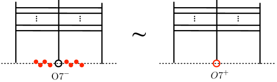
Figure 5: Freezing: O7${}^{-}+8$D7$|_{\textrm{fixed}}\sim\$O7⁺. Here, D7-branes are denoted by red dots and the charges of the 5-brane are neglected to highlight the relation between an O7^±-plane with 8 D7-planes.

Freezing.

The cubic prepotential of SU($N$) gauge theory with an antisymmetric and eight fundamentals ($1\textbf{AS}+8\mathbf{F}$) given in (4) can be reduced to that with a symmetric ($1\textbf{Sym}$), as proposed in Hayashi:2023boy :

$$\mathcal{F}_{\mathrm{SU}(N)_{\kappa}+1\textbf{AS}+(8+N_{f})\mathbf{F}}=\mathcal{F}_{\mathrm{SU}(N)_{\kappa}+1\textbf{Sym}+N_{f}\mathbf{F}}\ .$$ (12)

Though for simplicity, we set the hypermultiplet masses to zero, but this relation is generic. With $m_{\mathbf{AS}}=m_{\mathbf{Sym}}=m$ for (anti-)symmetric hypermultiplets, $m_{\mathbf{F}}=\frac{m}{2}$ for the eight fundamental hypermultiplets, one can easily check (12). We also remark that as in Hayashi:2023boy ; Kim:2023qwh , there exists a set of mass parameters giving rise to the relation even at the level of the (refined) instanton partition function which will be discussed in the next subsection

$$\mathrm{SU}(N)_{\kappa}+1\textbf{AS}+8\mathbf{F}~{}\longrightarrow~{}\mathrm{SU}(N)_{\kappa}+1\textbf{Sym}\ .$$ (13)

We refer to this reduction procedure as the freezing Hayashi:2023boy .

From the perspective of Type IIB 5-brane webs, the freezing can be understood as follows. As explained, SU$(N)+1\textbf{AS}+8\mathbf{F}$ is constructed with eight D7-branes (flavors) and an O7^--plane at which a half NS5-brane is stuck, while $\textrm{SU}(N)+1\textbf{Sym}$ is constructed by a 5-brane web with an O7⁺-plane where a half NS5-brane is stuck. To realize the freezing, eight D7-branes are put at the position of the O7^--plane such that they are bound together to make a combination of O7${}^{-}+8$D7 which leads to the same charge and monodromy as an O7⁺-plane,

$$\textrm{O7}^{-}+8\,\textrm{D7}\Big{|}_{\textrm{fixed}}~{}\sim~{}\textrm{O7}^{+}.$$ (14)

In doing so, one finds that the prepotential for $\textrm{SU}(N)+1\textbf{AS}+8\mathbf{F}$ becomes identical to that for $\textrm{SU}(N)+1\textbf{Sym}$. The corresponding 5-brane configuration is depicted in figure 5.

The concept of freezing involves fixing the positions of eight D7-branes close to an O7^--plane, producing an effect analogous to that of an O7⁺-plane as if eight D7-branes and an O7^--plane are “frozen” to form an O7⁺-plane. For SU type gauge theories, the freezing is a procedure that tunes the masses of $1\textbf{AS}+8\mathbf{F}$ to convert the set of hypermultiplets into $1\textbf{Sym}$ while the Coulomb branch parameters are untouched.

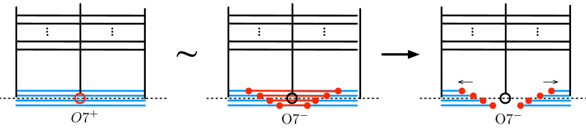
Figure 6: Unfreezing. $\mathsf{LEFT}$: A simplified 5-brane web for SU($2N+8)+1\textbf{Sym}$. Here, one brings four D5-branes (in blue) to the position of an O7⁺-plane and then one “unfreezes” an O7⁺-plane so that it can be effectively regarded as an O7^- and 8 D7s such that D7-branes are on the blue D5-branes. $\mathsf{MIDDLE}$: At the same time, four simultaneous Higgsing take place so that 8 D7-branes and 4 D5-branes in blue on top of O7^--plane are recombined such that D5-branes in red are suspended between two D7-branes. $\mathsf{RIGHT}$: The D5-branes in red are Higgsed away along $x^{7,8,9}$-directions and the remaining D7-branes attached to D5-branes in blue are taken to infinity so that the Hanany-Witten transition makes them free hypermultiplets. As a result, one obtains a 5-brane web for SU($2N)+1\textbf{AS}$.

Unfreezing.

We now imagine a reverse procedure of the freezing. Namely, we convert $1\textbf{Sym}$ into $1\textbf{AS}+8\mathbf{F}$, but we also simultaneously reduce the dimension of the Coulomb branch by the Higgsing discussed in (10):

$$\mathrm{SU}(N+8)_{\kappa}+1\textbf{Sym} ~{}\longrightarrow~{}\mathrm{SU}(N)_{\kappa}+1\textbf{AS}\ .$$ (15)

By setting all the unfrozen mass parameters to zero and at the same time performing four successive Higgsings with $a_{2N+1}=\cdots=a_{2N+8}=0$, one can see that the cubic prepotential yields

$$\mathcal{F}_{\mathrm{SU}(N+8)_{\kappa}+1\textbf{Sym}} ~{}\longrightarrow~{}\mathcal{F}_{\mathrm{SU}(N)_{\kappa}+1\textbf{AS}}\ .$$ (16)

This procedure can be viewed as “unfreezing”: we regard an O7⁺-plane effectively as O7^- paired with 8 D7s at fixed positions, which is at the same time followed by four consecutive Higgsings, each removing a configuration involving a color D5-brane connected to two D7-branes. Subsequent Hanany-Witten transitions Hanany:1996ie then displace the eight D7-branes from the vicinity of the O7^--plane along its monodromy cut, which makes eight D7s free hypermultiplets (or floating D7-branes). These procedures, depicted in figure 6, should take place at the same time.

We note that having discussed the freezings and unfreezings, one finds an intriguing relation between theories involving an O7-plane, which can be summarized as follows:

Figure 7: Freezing, unfreezing, and Higgsings for SU gauge theories.

We also remark that a similar relation arises for Sp/SO theories, which follows from the Higgsings of antisymmetric or symmetric hypermultiplet given in (7). More explicitly, one can see the relations as follows. Starting from the cubic prepotential for Sp($N+4$) theory with eight fundamental hypermultiplets. We freeze the theory by setting the masses of eight flavors to zero,

$$m_{N+1}=m_{N+2}=\cdots=m_{N+8}=0\ ,$$ (17)

which leads to the form of the prepotential given in (5), which is nothing but the prepotential for pure SO($2N+8$) theory:

$$\mathcal{F}_{\mathrm{Sp}(N+4)+8\mathbf{F}}\xrightarrow[\eqref{eq:massfreezingSptoSO}]{\textrm{freezing}}~{} \frac{1}{g_{0}^{2}}\sum_{i=1}^{N+4}a_{i}^{2}+\frac{1}{6}\sum_{i<j}^{N+4}\big{(}(a_{i}-a_{j})^{3}+(a_{i}+a_{j})^{3}\big{)}=\mathcal{F}_{\mathrm{SO}(2N+8)}\ .$$ (18)

We then do the unfreezing by setting $a_{N+j}=0$ ($j=1,2,3,4$) which leads to the cubic prepotential for pure Sp($N$) theory:

$$\mathcal{F}_{\mathrm{SO}(2N+8)}\xrightarrow{\textrm{unfreezing}} ~{}\frac{1}{g_{0}^{2}}\sum_{i=1}^{N}a_{i}^{2}+\frac{1}{6}\sum_{i<j}^{N}\!\big{(}(a_{i}\!-\!a_{j})^{3}+(a_{i}\!+\!a_{j})^{3}\big{)}\!+\!\frac{8}{6}\sum_{i=1}^{N}a_{i}^{3}=\mathcal{F}_{\mathrm{Sp}(N)}\ .$$ (19)

Together with a successive application of conventional Higgsing, $\operatorname{Sp}(N+4)+8F\to\operatorname{Sp}(N)$, one can summarize the relation between $\operatorname{Sp}/\operatorname{SO}$ gauge theories as follows:

Figure 8: Freezing, unfreezing, and Higgsings for Sp/SO gauge theories.

Because these various intriguing relations between theories involving an O7^±-plane are presented based on the cubic prepotentials, one is tempted to speculate whether the same relation holds even at the non-perturbative level. It is suggestive that though the cubic prepotential only captures perturbative aspects, the existence of the corresponding brane configurations would imply that a similar relation can be extended to the non-perturbative level. We now consider 5d instanton partition functions on the $\Omega$-background and generalize the freezing with refined $\Omega$-deformation parameters, $\epsilon_{1,2}$.

2.2 Identities of 5d instanton partition functions

In 5d supersymmetric theories, one of the most important observables is an instanton partition function Nekrasov:2002qd on $S^{1}\times\mathbb{R}^{4}$ with the $\Omega$-background. It is defined as an index that counts BPS states within a 5d theory:

$$Z_{\textrm{inst}}\left(\epsilon_{1},\epsilon_{2},a_{i},m\right)=\operatorname{Tr}\left[(-1)^{\mathsf{F}}e^{-\beta\left\{Q,Q^{\dagger}\right\}}e^{-\epsilon_{1}\left(J_{1}+J_{R}\right)}e^{-\epsilon_{2}\left(J_{2}+J_{R}\right)}e^{-a_{i}C_{i}}e^{-m\cdot F}\right]\ .$$ (20)

Here, $J_{1},J_{2}$ are defined by the Cartans $J_{l},J_{r}$ of the spacetime symmetry $\operatorname{SO}(4)\cong\operatorname{SU}(2)_{l}\times\operatorname{SU}(2)_{r}$ of $\mathbb{R}^{4}$ via $J_{1}=\frac{J_{r}+J_{l}}{2},J_{2}=\frac{J_{r}-J_{l}}{2}$. The operator $J_{R}$ represents the Cartan generator of the $\operatorname{SU}(2)_{R}$ R-symmetry. The Coulomb branch parameters are denoted as $a_{i}$, where the index $i$ ranges from 1 to the rank of the gauge group $G$. All additional flavor symmetries are collectively labeled as $F$, which are conjugate to the mass parameters $m$.

Instantons, representing non-perturbative effects in gauge theories, play a crucial role in understanding the behavior of gauge theories in strong coupling regimes, where traditional perturbative methods fail. The method employed by Nekrasov Nekrasov:2002qd involved localization techniques, which allowed the path integral of the gauge theory to be exactly computed by localizing it to the moduli space of instantons. Consequently, the instanton partition function can be understood as a character of the equivariant action

$$\mathbb{C}_{\epsilon_{1}}^{\times}\times\mathbb{C}_{\epsilon_{2}}^{\times}\times\prod_{i}^{\operatorname{rk}G}\mathbb{C}_{a_{i}}^{\times}\times\prod_{j}^{\operatorname{rk}F}\mathbb{C}_{m_{j}}^{\times}~{}.$$ (21)

on the instanton moduli spaces. A more physical perspective interprets it that a 5d theory on the $\Omega$-background effectively localizes to supersymmetric quantum mechanics on the instanton moduli spaces, and (20) is its partition function. As exact results, encoding all non-perturbative effects in a gauge theory, we make use of the instanton partition functions to see the consequence of freezing and unfreezing.

First, let us recall the Higgsing of $\operatorname{SU}(N)_{\kappa}+1\textbf{Sym}$ to $\operatorname{SO}(N)$ at the level of instanton partition functions Chen:2023smd . Turning on the $\Omega$-background, a brane may change its position by a certain linear combination of $\epsilon_{1,2}$ from the absence of the background. As in figure 2, to Higgs $\operatorname{SU}(N)_{\kappa}+1\textbf{Sym}$ to $\operatorname{SO}(N)$, all the D5-branes are aligned and the middle NS5-brane is positioned at $\epsilon_{+}/2$ so that we tune the parameters of the theory

$$m=\epsilon_{+}~{},\qquad a_{N-i+1}=-a_{i}~{},$$ (22)

where $m$ is the mass of the symmetric hypermultiplet. Note that when $N$ is odd, we set $a_{\frac{N+1}{2}}=0$. At this specialization, the instanton partition function behaves

$$Z_{2k,\kappa=\frac{1}{2}(N\bmod 2)}^{\operatorname{SU}(N)+1\textbf{Sym}}\ \xrightarrow[\eqref{SU-SO-Higgsing}]{\textrm{Higgsing}}\ (-1)^{k(N+1)}Z_{k}^{\operatorname{SO}(N)}~{},$$ (23)

for $N\geq 4$. It is important to note that $2k$-instanton on the left-hand side coincides with $k$-instanton on the right-hand side, and the odd-instanton partition functions of $\operatorname{SU}(N)_{\kappa}+1\textbf{Sym}$ vanish at the specialization (22).

We can apply a similar procedure to the brane configuration involving an O7^--plane ($\operatorname{SU}(N)_{\kappa}+1\textbf{AS}$) to obtain the brane configuration for pure $\operatorname{Sp}(N)$ gauge theory, as given in figure 1. This involves the specialization

$$m=\epsilon_{+}~{},\qquad a_{2N-i+1}=-a_{i}~{},$$ (24)

manipulating the instanton partition functions, which yields the following identities:

$$Z_{k,\kappa\equiv N\bmod 2}^{\operatorname{SU}(2N)+1\textbf{AS}}\ \xrightarrow[\eqref{SU-Sp-Higgsing}]{\textrm{Higgsing}} \ (-1)^{k(N+1)+\lceil\frac{k}{2}\rceil}Z_{k,\theta=0}^{\operatorname{Sp}(N)}\ ,$$ (25)

$$Z_{k,\kappa\equiv N+1\bmod 2}^{\operatorname{SU}(2N)+1\textbf{AS}}\ \xrightarrow[\eqref{SU-Sp-Higgsing}]{\textrm{Higgsing}} \ (-1)^{k(N+1)+\lceil\frac{k}{2}\rceil}Z_{k,\theta=\pi}^{\operatorname{Sp}(N)}\ .$$

The value of the discrete $\theta$-angle in the resulting $\operatorname{Sp}(N)$ theory is determined by both the Chern-Simons level and the rank of the gauge group.

SU($N$) gauge theories with (anti-)symmetric hypermultiplet

In the context of instanton partition functions, we apply the Higgsing process as depicted in figure 4 to reduce the rank of a gauge group. It is important to note that, on the $\Omega$-background, the positions of branes, which correspond to the Coulomb branch and mass parameters, might be shifted by a linear combination of $\epsilon_{1,2}$. Particularly, the Higgsing of the $\operatorname{SU}(N)_{\kappa}+1\textbf{AS}+N_{f}\mathbf{F}$ instanton partition function à la figure 4 can be implemented using two distinct sets of parameterizations. One such set of parameters is defined as

$$a_{N}=-a_{N-1}-m-\epsilon_{+},\quad m_{N_{f}}=-a_{N-1}+\epsilon_{+},\quad m_{N_{f}-1}=a_{N-1}+m+2\epsilon_{+}~{},$$ (26)

and an alternate set is obtained by changing $\epsilon_{i}\to-\epsilon_{i}$ above. Under these conditions, one can verify that the instanton partition function of $\operatorname{SU}(N)_{\kappa}+1\textbf{AS}+N_{f}\mathbf{F}$ reduces both the gauge group rank and the number of fundamental hypermultiplets by two:

$$Z^{\operatorname{SU}(N)_{\kappa}+1\textbf{AS}+N_{f}\textbf{F}}_{\textrm{inst}}\ \xrightarrow[\eqref{Higgsing-parameters}]{\textrm{Higgsing}}\ Z^{\operatorname{SU}(N-2)_{\kappa}+1\textbf{AS}+(N_{f}-2)\textbf{F}}_{\textrm{inst}}~{},$$ (27)

which can be checked at the level of the integrand:

$$\mathcal{Z}_{\operatorname{SU}(N)_{\kappa},k}^{\textrm{vec}}\mathcal{Z}_{\operatorname{SU}(N),k}^{\textrm{anti}}(m)\mathcal{Z}_{\operatorname{SU}(N),k}^{N_{f}}\Big{|}_{\eqref{Higgsing-parameters}}=\mathcal{Z}_{\operatorname{SU}(N-2)_{\kappa},k}^{\textrm{vec}}\mathcal{Z}_{\operatorname{SU}(N-2),k}^{\textrm{anti}}(m)\mathcal{Z}_{\operatorname{SU}(N-2),k}^{N_{f}-2}\ .$$ (28)

The various contributions to the ADHM integrals are summarized in appendix B.

Now let us consider the effect of freezing (14) on the instanton partition functions for $\operatorname{SU}(N)_{\kappa}+1\textbf{AS}+8\textbf{F}$ whose brane setting is explained in the previous section. On a generic $\Omega$-background, we apply the freezing $8\mathrm{D}7$ to O7^- by setting the mass parameters $m_{\ell=1,\cdots,8}$ of eight fundamental hypermultiplets to

$$m_{\ell}=\frac{m\pm\epsilon_{\pm}}{2}(+\pi i)\ ,$$ (29)

where $m$ is the mass of an antisymmetric hypermultiplet. (See also our notation convention in Appendix A.) Here, we consider all possible combinations of signs, and $(+\pi i)$ indicates both the inclusion and exclusion of this shift. Upon the freezing, the instanton partition function reduces to that of $\operatorname{SU}(N)_{\kappa}+1\textbf{Sym}$

$$Z^{\operatorname{SU}(N)_{\kappa}+1\textbf{AS}+8\textbf{F}}_{\textrm{inst}}\ \xrightarrow[\eqref{AS-to-S}]{\textrm{freezing }}\ Z^{\operatorname{SU}(N)_{\kappa}+1\textbf{Sym}}_{\textrm{inst}}~{}.$$ (30)

This can be shown by comparing the integrands of the instanton partition functions at each instanton level, without performing JK-residues. Using the identity (144), one can verify that

$$\mathcal{Z}_{\operatorname{SU}(N)_{\kappa},k}^{\textrm{vec}}\mathcal{Z}_{\operatorname{SU}(N),k}^{\textrm{anti}}(m)\mathcal{Z}_{\operatorname{SU}(N),k}^{N_{f}=8}\Big{|}_{\eqref{AS-to-S}}=\mathcal{Z}_{\operatorname{SU}(N)_{\kappa},k}^{\textrm{vec}}\mathcal{Z}_{\operatorname{SU}(N),k}^{\textrm{sym}}(m)\ .$$ (31)

Therefore, the identity (30) holds when we introduce the same 5d Chern-Simons term to the two theories.

For unfreezing, there are notable differences compared to the prepotential case (16). While we tune the positions of only eight color branes for prepotential, we need more color branes and flavor branes for unfreezing at the level of instanton partition functions. This is because the positions (29) of 8D7 are different from each other. To Higgs these 8D7 branes, we require the introduction of eight more color branes and an equal number of additional D7 branes, leading to the following

$$Z^{\operatorname{SU}(N+16)_{\kappa}+1\textbf{Sym}+8\textbf{F}}_{\textrm{inst}}\ \xrightarrow[\eqref{S-to-AS}]{\textrm{Unfreezing}}\ Z^{\operatorname{SU}(N)_{\kappa}+1\textbf{AS}}_{\textrm{inst}}~{},$$ (32)

which can be executed by two different parameter specializations. One such set of parameters is given by

$$a_{s}=-\frac{m}{2}-\epsilon_{+}\pm\frac{\epsilon_{\pm}}{2}(+\pi i),\quad-\frac{m}{2}+2\epsilon_{+}\pm\frac{\epsilon_{\pm}}{2}(+\pi i)$$ (33)

$$m_{l}=\frac{m}{2}-3\epsilon_{+}\pm\frac{\epsilon_{\pm}}{2}(+\pi i)\ ,$$ (34)

and the other set is obtained by changing $\epsilon_{i}\to-\epsilon_{i}$ above. The other set is obtained by changing $\epsilon_{i}\to-\epsilon_{i}$ above. As detailed in (26), there are two parametrizations for Higgsing of the instanton partition function, leading to the above two transformations. This can be confirmed, in a similar manner to (31), by examining the identity of the ADHM integrands at each instanton level.

We remark that if one combines the two processes, Freezing and Unfreezings, together, the total effect is equivalent to eight sequential Higgsings of (27), which is illustrated in figure 9. Moreover, during the unfreezing process, the instanton partition function exhibits a sudden jump. This novel phenomenon will be treated in section 2.4 in detail.

Figure 9: This figure illustrates the relationships between refined instanton partition functions for SU gauge groups under specific parameter specializations. It shows that the partition function $Z^{\mathrm{SU}(N+16)_{\kappa}+1\textbf{AS}+16\textbf{F}}_{k}$, following the freezing process (29), becomes identical to $Z^{\mathrm{SU}(N+16)_{\kappa}+1\textbf{Sym}+8\mathbf{F}}_{k}$. Additionally, when the unfreezing procedures (33) are applied, $Z^{\mathrm{SU}(N+16)_{\kappa}+1\textbf{Sym}+8\mathbf{F}}_{k}$ corresponds to $Z^{\mathrm{SU}(N)_{\kappa}+1\textbf{AS}}_{k}$. The dashed line in the figure represents BPS jumping.

Sp($N$) and SO($2N$) gauge theories

As demonstrated in (23) and (25), the Higgsing applied to $\operatorname{SU}(2N)+1\textbf{Sym}$ or $\operatorname{SU}(2N)+1\textbf{AS}$ transitions into pure Yang-Mills theory for either $\operatorname{SO}(2N)$ or $\operatorname{Sp}(N)$ gauge group. Consequently, this Higgsing process, as outlined in (24), alongside the subsequent steps of freezing and unfreezing, establishes a connection between the instanton partition functions of the $\operatorname{Sp}(N)$ and $\operatorname{SO}(2N)$ gauge theories. Let us look at this relationship more closely.

We start the $\operatorname{Sp}(N)_{\theta}+8\mathbf{F}$ setup, where eight mass parameters are specifically arranged for the freezing process as follows:

$$m_{\ell}~{}=~{}0,~{}~{}\epsilon_{+},~{}~{}\frac{\epsilon_{1,2}}{2},~{}~{}\pi i,~{}~{}\epsilon_{+}+\pi i,~{}~{}\frac{\epsilon_{1,2}}{2}+\pi i\ .$$ (35)

These parameterizations can be seen as the $m=\epsilon_{+}$ specialization of (29). When we apply this freezing process, the $2k$-instanton partition function of $\operatorname{Sp}(N)_{\theta}+8\mathbf{F}$ becomes identical to the $k$-instanton partition function of the pure $\operatorname{SO}(2N)$ Yang-Mills

$$Z^{\operatorname{Sp}(N)_{\theta}+8\textbf{F}}_{2k}\ \xrightarrow[\eqref{Sp-to-SO-para}]{\textrm{freezing }}\ Z^{\operatorname{SO}(2N)}_{k}~{}.$$ (36)

Interestingly, this process of freezing, particularly the setting of one fundamental mass to zero, eliminates the minus sector from the $\operatorname{Sp}(N)$ instanton partition function, as indicated in (166). Consequently, this freezing process is independent of a choice of the discrete $\theta$-angle, and we can verify it from the identity of the ADHM integrands

$$\mathcal{Z}_{\mathrm{Sp}(N),2k}^{\mathrm{vec},+}\mathcal{Z}_{\mathrm{Sp}(N),2k}^{N_{f}=8,+}\Big{|}_{\eqref{Sp-to-SO-para}}=\mathcal{Z}_{\mathrm{SO}(2N),k}^{\mathrm{vec}}~{}.$$ (37)

The subsequent stages of unfreezing become more subtle. As mentioned above, the freezing process (35) removes the minus sector of the $\operatorname{Sp}(N)$ instanton partition function because one of the fundamental masses is set to be zero $m_{\ell}=0$. The processes of unfreezing then revive the plus sector with even instanton numbers:

$$Z_{k}^{\mathrm{SO}(2N+16)+8\mathbf{F}}\xrightarrow[\eqref{SO-to-Sp}]{\textrm{unfreezing}}Z_{2k}^{\mathrm{Sp}(N)^{+}}\ ,$$ (38)

adjusting the Coulomb branch ($a_{s}$) and mass parameters ($m_{\ell}$) as follows:

$$a_{s}= ~{}0,~{}~{}\epsilon_{+},~{}~{}\frac{\epsilon_{1,2}}{2},~{}~{}\pi i,~{}~{}\epsilon_{+}+\pi i,~{}~{}\frac{\epsilon_{1,2}}{2}+\pi i,$$ (39)

$$m_{l}= ~{}a_{s}+\epsilon_{+}.$$ (40)

By increasing the rank of the gauge group and the number of fundamental masses, other sectors of the $\operatorname{Sp}(N)$ instanton partition function can be accessed through unfreezing. The details are committed, but these can be also verified at the level of the integrand (up to some factor):

$$Z_{k}^{\mathrm{SO}(2N+18)+10\mathbf{F}} \xrightarrow{\textrm{unfreezing}}Z_{2k+1}^{\mathrm{Sp}(N)^{+}}$$ (41)

$$a_{s}=0(+\pi i)~{},\ \epsilon_{+}(+\pi i)~{},\ \frac{\epsilon_{1.2}}{2}(+\pi i)~{},\ \epsilon_{-}$$ (42)

$$m_{l}=\epsilon_{+}(+\pi i)~{},\ 2\epsilon_{+}(+\pi i)~{},\ \epsilon_{+}+\frac{\epsilon_{1\cdot 2}}{2}(+\pi i)~{},\ 0,\,\ 2\epsilon_{+}.$$ (43)

$$Z_{k}^{\mathrm{SO}(2N+18)+10\mathbf{F}} \xrightarrow{\textrm{unfreezing}}Z_{2k+1}^{\mathrm{Sp}(N)^{-}}$$ (44)

$$a_{s}=0(+\pi i)~{},\ \epsilon_{+}(+\pi i)~{},\ \frac{\epsilon_{1.2}}{2}(+\pi i)~{},\ \epsilon_{-}+\pi i$$ (45)

$$m_{l}=\epsilon_{+}(+\pi i)~{},\ 2\epsilon_{+}(+\pi i)~{},\ \epsilon_{+}+\frac{\epsilon_{1\cdot 2}}{2}(+\pi i)~{},\ \pi i,\,\ 2\epsilon_{+}+\pi i.$$ (46)

$$Z_{k-1}^{\mathrm{SO}(2N+20)+12\mathbf{F}} \xrightarrow{\textrm{unfreezing}}Z_{2k}^{\mathrm{Sp}(N)^{-}}$$ (47)

$$a_{s}=0(+\pi i)~{},\ \epsilon_{+}(+\pi i)~{},\ \frac{\epsilon_{1.2}}{2}(+\pi i)~{},\ \epsilon_{-}(+\pi i)$$ (48)

$$m_{l}=\epsilon_{+}(+\pi i)~{},\ 2\epsilon_{+}(+\pi i)~{},\ \epsilon_{+}+\frac{\epsilon_{1\cdot 2}}{2}(+\pi i)~{},\ 0(+\pi i),\,\ 2\epsilon_{+}(+\pi i).$$ (49)

Comments on 4d instanton partition functions

While we have focused on 5d instanton partition functions so far, let us make brief comments on 4d instanton partition functions. In fact, from 5d to 4d instanton partition functions, we can simply make the following replacements

$$\operatorname{sh}(\alpha)\rightarrow\alpha~{},\qquad\operatorname{ch}(\alpha)\rightarrow 2~{}.$$ (51)

To implement the freezing process in the NS5-D4-D6-O6 system within Type IIA, we position four D6-branes at the location of the O6^--plane. These D6-branes are bound together, forming a composite structure of O6${}^{-}+4$D6. The resulting effect can be compared with that of an O6⁺-plane:

$$\textrm{O6}^{-}+4\,\textrm{D6}\Big{|}_{\textrm{fixed}}~{}\sim~{}\textrm{O6}^{+}.$$ (52)

(For a more detailed explanation, refer to section 3.1.) This leads to the identity of 4d instanton partition functions of $\operatorname{SU}(N)+1\textbf{AS}+4\mathbf{F}$ and $\operatorname{SU}(N)+1\textbf{Sym}$ where the mass parameters are as in (29) without $(+\pi i)$ shifts. Similarly, the unfreezing process in this setting provides the identity of 4d instanton partition functions of $\operatorname{SU}(N+8)+1\textbf{Sym}+4\mathbf{F}$ and $\operatorname{SU}(N)+1\textbf{AS}$ where the parameter specializations are as in (33) again without $(+\pi i)$ shifts. It becomes evident that the (un)freezing process also implicates identities between 4d $\operatorname{SO}(N)$ and $\operatorname{Sp}(N)$ instanton partition functions, although we will omit the details here.

2.3 E-string $\to$ M-string

Up to this point, our study revealed a striking correspondence in the instanton partition functions. Specifically, we have found that, as a result of freezing, the partition function for $\text{SU}(N)_{\kappa}+1\textbf{AS}+8\mathbf{F}$ coincides with that of $\text{SU}(N)_{\kappa}+1\textbf{Sym}$, upon the eight masses of the fundamentals are appropriately tuned. This finding not only enhances our understanding of instanton dynamics but also bridges different configurations in string theory.

A particularly intriguing manifestation of this correspondence is found in the context of E-string Witten:1995gx ; Ganor:1996mu ; Seiberg:1996vs and M-string Haghighat:2013gba theories. Although these theories have 6d origins, they admit 5d realizations, offering a unique playground to explore the above correspondence. In this respect, the E-string theory is effectively disguised as a 5d SU(2) theory with eight fundamental hypermultiplets, while M-string theory reveals itself as a 5d SU(2) theory of the discrete theta $\theta=0$ with one symmetric (adjoint) hypermultiplet:

$$\textrm{E-string on }S^{1}= \textrm{ 5d SU(2)+8{F}}\ ,$$ (53)

$$\textrm{M-string on }S^{1}= \textrm{ 5d SU(2)${}_{0}$+1{Sym}}\ .$$

Therefore, while the partition functions of E-string and M-string have been computed by various methods Haghighat:2013gba ; Haghighat:2014pva ; Kim:2014dza ; Cai:2014vka ; Kim:2015jba ; Kim:2017jqn ; Kim:2020hhh ; Kim:2022dbr , we can make use of 5d instanton partition functions to evaluate them here as in Hwang:2014uwa . Since the antisymmetric representation of SU(2) is trivial, the $N=2$ specialization (30) of the freezing effect can be understood as the relation between E-string and M-string through this approach. Namely, upon specializing the eight mass parameters in E-string, the partition function agrees remarkably with that of M-string.

Poles at infinity and brane diagrams

Before delving into the partition functions of E-string and M-string theory, it is important to discuss a pole at infinity in the ADHM integrand and its interpretation in a brane diagram. As figure 10 depicts, the external 5-branes meet at a certain point in the 5-brane web diagram for SU(2)+1Sym, and a D1-brane suspended by these external 5-branes is bounced back. In such scenarios, the ADHM instanton integrals suffer from higher-order poles at infinity. For example, the expression for the 1-instanton case from (147),

$$\mathcal{Z}^{\operatorname{SU}(2)_{0}+1\textbf{Sym}}_{k=1}=\frac{\operatorname{sh}(\phi+m\pm a)\operatorname{sh}(\pm({m}+2\phi)-\epsilon_{-})\operatorname{sh}(2\epsilon_{+})}{\operatorname{sh}(\epsilon_{1,2})\operatorname{sh}(\epsilon_{+}\pm{a}\pm\phi)}~{}\overset{\phi\to\infty}{\sim}~{}\mathcal{O}(e^{\phi})\ ,$$ (54)

shows the presence of a higher-order pole as $\phi\to\infty$. This issue is present even for higher instantons. A similar issue arises in the instanton partition function for SU(2)+1AS+8F. As a result, a naive application of the JK residue method fails to yield the correct partition function.

Figure 10: $\mathsf{LEFT}$: the brane diagram for SU(2) with one symmetric hypermultiplet. $\mathsf{RIGHT}$: the brane diagram for Sp(1) with eight fundamental hypermultiplets. The external 5-branes meet at a certain point in both diagrams, which indicates the presence of a higher-order pole at infinity in ADHM integrands.

1-instanton

For SU(2)₀+1Sym, we can use the expression for the adjoint hypermultiplet in (147) since $\textbf{Sym}\cong\textbf{Adj}$ for SU(2). For instance, the 1-instanton part behaves as

$$\mathcal{Z}_{k=1}^{\operatorname{SU}(2)_{0}+1\textbf{Adj}}=\frac{\operatorname{sh}(m\pm\phi\pm a)\operatorname{sh}(\epsilon_{-}\pm m)\operatorname{sh}(2\epsilon_{+})}{\operatorname{sh}(\epsilon_{1,2})\operatorname{sh}(\epsilon_{+}\pm{a}\pm\phi)}~{}\overset{\phi\to\infty}{\sim}~{}\mathcal{O}(1)\ .$$ (55)

Therefore, the JK residue integral provides

$$Z_{k=1}^{\operatorname{SU}(2)_{0}+1\textbf{Adj}}= ~{}\frac{\operatorname{sh}(m\pm(2a-\epsilon_{+}))\operatorname{sh}(m\pm\epsilon_{-})}{\operatorname{sh}(\epsilon_{1,2})\operatorname{sh}(2{a})\operatorname{sh}(2\epsilon_{+}-2{a})}$$ (56)

$$+\frac{\operatorname{sh}(m\pm(2a+\epsilon_{+}))\operatorname{sh}(m\pm\epsilon_{-})}{\operatorname{sh}(\epsilon_{1,2})\operatorname{sh}(-2{a})\operatorname{sh}(2\epsilon_{+}+2{a})}$$

$$= ~{}Z_{\textrm{extra},k=1}^{\operatorname{SU}(2)_{0}+1\textbf{Adj}}+Z_{\textrm{QFT},k=1}^{\operatorname{SU}(2)_{0}+1\textbf{Adj}}\ ,$$

where $Z_{\textrm{extra}}$ is the part independent of the Coulomb branch parameter, $a$,

$$Z_{\textrm{extra},k=1}^{\operatorname{SU}(2)_{0}+1\textbf{Adj}}= ~{}2\frac{\operatorname{sh}(m\pm\epsilon_{-})}{\operatorname{sh}(\epsilon_{1,2})}~{},$$ (57)

$$Z_{\textrm{QFT},k=1}^{\operatorname{SU}(2)_{0}+1\textbf{Adj}}= ~{}\frac{\operatorname{sh}(\epsilon_{\pm}\pm m)\operatorname{ch}(2\epsilon_{+})}{\operatorname{sh}(\epsilon_{1,2})\operatorname{sh}(2\epsilon_{+}\pm 2a)}\ .$$

Now let us turn to E-string theory. The ADHM integrand of SU(2)+8F obtained from (147) exhibits a higher-order pole $\mathcal{O}(e^{2\phi})$ at infinity. In contrast, the ADHM integrand of $\operatorname{Sp}(1)_{\theta=0}+8\textbf{F}$, derived from the formulas in appendix B.3, presents a less severe singularity $\mathcal{O}(e^{\phi})$ at infinity (see the right of figure 10) although it provides the same partition function as SU(2)+8F. This makes the latter more manageable. To mitigate the singularity at infinity, we can make use of an antisymmetric hypermultiplet Hwang:2014uwa ; Gaiotto:2015una ; Chen:2021ivd . For the $\operatorname{SU}(2)\cong\operatorname{Sp}(1)$ gauge group, the antisymmetric representation is trivial, meaning the addition of an antisymmetric hypermultiplet does not fundamentally change the physics. However, this addition is beneficial as the contribution of the antisymmetric hypermultiplet tends towards $\mathcal{O}(e^{-\phi})$ at infinity, therefore softening the singularity. Thus, to derive the E-string partition function, we will examine the ADHM instanton partition function of $\operatorname{Sp}(1)_{0}$+1AS+8F in detail because it behaves as $\mathcal{O}(1)$ at infinity.

At 1-instanton, the ADHM instanton partition function of $\operatorname{Sp}(1)_{0}$+1AS+8F does not involve an integral Shadchin:2005mx ; Kim:2012gu so that the evaluation is straightforward:

$$Z_{k=1}^{\operatorname{Sp}(1)_{0}+1\textbf{AS}+8\textbf{F}}= ~{}Z_{k=1}^{\operatorname{Sp}(1)_{0}+1\textbf{AS}+8\textbf{F},+}+Z_{k=1}^{\operatorname{Sp}(1)_{0}+1\textbf{AS}+8\textbf{F},-}$$ (58)

$$= ~{}\frac{\operatorname{sh}(\pm a+m)\prod_{\ell=1}^{8}\operatorname{sh}(m_{\ell})}{\operatorname{sh}(\epsilon_{1,2})\operatorname{sh}(\pm m-\!\epsilon_{+})\operatorname{sh}(\pm a+\epsilon_{+})}\!+\!\frac{\operatorname{ch}(\pm a+m)\prod_{\ell=1}^{8}\operatorname{ch}(m_{\ell})}{\operatorname{ch}(\epsilon_{1,2})\operatorname{ch}(\pm m-\!\epsilon_{+})\operatorname{ch}(\pm a+\epsilon_{+})}$$

$$= ~{}Z_{\textrm{extra},k=1}^{\operatorname{Sp}(1)_{0}+1\textbf{AS}+8\textbf{F}}+Z_{\textrm{QFT},k=1}^{\operatorname{Sp}(1)_{0}+1\textbf{AS}+8\textbf{F}}\ ,$$

where, in the last line, we separate the parts dependent (labelled by QFT) and independent (labelled by extra) of the Coulomb branch parameter:

$$Z_{\textrm{QFT},k=1}^{\operatorname{Sp}(1)_{0}+1\textbf{AS}+8\textbf{F}}=-\frac{\prod_{\ell=1}^{8}\operatorname{sh}(m_{\ell})}{\operatorname{sh}(\epsilon_{1,2})\operatorname{sh}(\pm a+\epsilon_{+})}-\frac{\prod_{\ell=1}^{8}\operatorname{ch}(m_{\ell})}{\operatorname{ch}(\epsilon_{1,2})\operatorname{ch}(\pm a+\epsilon_{+})}~{},$$ (59)

$$Z_{\textrm{extra},k=1}^{\operatorname{Sp}(1)_{0}+1\textbf{AS}+8\textbf{F}}=\frac{\prod_{\ell=1}^{8}\operatorname{sh}(m_{\ell})}{\operatorname{sh}(\epsilon_{1,2})\operatorname{sh}(\pm m-\epsilon_{+})}+\frac{\prod_{\ell=1}^{8}\operatorname{ch}(m_{\ell})}{\operatorname{ch}(\epsilon_{1,2})\operatorname{ch}(\pm m-\epsilon_{+})}~{}.$$

Upon specializing the eight masses $m_{\ell}$ as in (29), we obtain

$$Z_{\textrm{QFT},k=1}^{\operatorname{Sp}(1)_{0}+1\textbf{AS}+8\textbf{F}}\Big{|}_{\eqref{AS-to-S}}=-\frac{\operatorname{sh}(\epsilon_{\pm}\pm m)\operatorname{ch}(2\epsilon_{+})}{\operatorname{sh}(\epsilon_{1,2})\operatorname{sh}(2\epsilon_{+}\pm 2a)}\ .$$ (60)

Comparing this with (57), we see a relationship between the 1-instanton partition functions of the E-string and M-string,

$$Z_{\textrm{QFT},k=1}^{\operatorname{Sp}(1)_{0}+1\textbf{AS}+8\textbf{F}}\ \xrightarrow[]{\eqref{AS-to-S}}\ -Z_{\textrm{QFT},k=1}^{\operatorname{SU}(2)_{0}+1\textbf{Adj}}~{}.$$ (61)

Higher-instanton

Let us move on to higher-instanton. The instanton partition function of SU(2)₀+1Adj Nekrasov:2002qd ; Bruzzo:2002xf can be expressed in terms of sums over Young diagrams as

$$Z^{\operatorname{SU}(2)_{0}+1\textbf{Adj}}=\sum_{k\geq 0}e^{-m_{0}k}\!\!\!\!\sum_{\sum_{s}|\lambda^{(s)}|=k}\,\prod_{s,t=1}^{2}\prod_{x\in\lambda^{(s)}}\,\frac{\operatorname{sh}(N_{st}+m-\epsilon_{+})\operatorname{sh}(N_{st}-m-\epsilon_{+})}{\operatorname{sh}(N_{st})\operatorname{sh}(N_{st}-2\epsilon_{+})},$$ (62)

where $m_{0}$ is the inverse coupling squared (or instanton mass), and we define the Nekrasov factor as

$$N_{st}(x)=a_{s}-a_{t}-\epsilon_{1}L_{\lambda^{(s)}}(x)+\epsilon_{2}(A_{\lambda^{(t)}}(x)+1)~{}.$$ (63)

(See (140) for the definitions of the arm $A_{\lambda}(x)$ and leg $L_{\lambda}(x)$ length for a content $x\in\lambda$.) As seen above, this can be factored into two parts

$$Z^{\operatorname{SU}(2)_{0}+1\textbf{Adj}}=Z_{\textrm{extra}}^{\operatorname{SU}(2)_{0}+1\textbf{Adj}}Z_{\textrm{QFT}}^{\operatorname{SU}(2)_{0}+1\textbf{Adj}}~{},$$ (64)

where $Z_{\textrm{extra}}^{\operatorname{SU}(2)_{0}+1\textbf{Adj}}$ is expressed in terms of a plethystic exponential

$$Z_{\textrm{extra}}^{\operatorname{SU}(2)_{0}+1\textbf{Adj}}=\textrm{PE}\left[\frac{e^{-m_{0}}}{1-e^{-m_{0}}}\frac{2\operatorname{sh}(m\pm\epsilon_{-})}{\operatorname{sh}(\epsilon_{1,2})}\right]~{}.$$ (65)

On the other hand, a closed-form expression of the refined instanton partition function of $\operatorname{Sp}(1)_{0}$+1AS+8F is unavailable because it is difficult to classify the JK pole structure. Therefore, we perform the JK residue integral at each instanton level. To extract a genuine instanton contribution, it is necessary to eliminate the extra factor that is independent of the Coulomb branch parameter. For the sake of simplicity, we focus on the extra factor specifically at the specialization (29), as a computation for generic mass parameters is computationally intensive:

$$Z^{\operatorname{Sp}(1)_{0}+1\textbf{AS}+8\textbf{F}}\Big{|}_{\eqref{AS-to-S}}=Z_{\textrm{extra}}^{\operatorname{Sp}(1)_{0}+1\textbf{AS}+8\textbf{F}}\cdot Z_{\textrm{QFT}}^{\operatorname{Sp}(1)_{0}+1\textbf{AS}+8\textbf{F}}\Big{|}_{\eqref{AS-to-S}}~{},$$ (66)

where $Z_{\textrm{extra}}^{\operatorname{Sp}(1)_{0}+1\textbf{AS}+8\textbf{F}}$ is expressed in terms of a plethystic exponential

$$Z_{\textrm{extra}}^{\operatorname{Sp}(1)_{0}+1\textbf{AS}+8\textbf{F}}=\textrm{PE}\left[\frac{e^{-m_{0}}}{1+e^{-m_{0}}}\frac{\operatorname{sh}(\epsilon_{-}\pm m)}{\operatorname{sh}(\epsilon_{1,2})}\bigg{(}1-\frac{e^{-m_{0}}}{1-e^{-m_{0}}}\frac{\operatorname{ch}(2\epsilon_{+})}{2\operatorname{ch}(m\pm\epsilon_{+})}\bigg{)}\right]~{}.$$ (67)

We have verified the equivalence of the partition functions up to $k=4$ at the refined level (up to sign):

$$Z_{\textrm{QFT},k}^{\operatorname{Sp}(1)_{0}+1\textbf{AS}+8\textbf{F}}\Big{|}_{\eqref{AS-to-S}}=(-1)^{k}Z_{\textrm{QFT},k}^{\operatorname{SU}(2)_{0}+1\textbf{Adj}}~{}.$$ (68)

We remark that in a similar fashion, one can also take another freezing limit on the E-string partition function which leads to the partition function for $\operatorname{SU}(2)_{\pi}+1\mathbf{Adj}$. The map is based on Kim:2023qwh and given by:

$$m_{1,\cdots,8}=\pm\frac{m+\epsilon_{+}}{2},~{}~{}\frac{m\pm\epsilon_{-}}{2},~{}~{}\frac{m\pm\epsilon_{\pm}}{2}+\pi i\ ,$$ (69)

where $m$ is the mass of the adjoint hypermultiplet.

The two different freezings on E-string were also checked in Kim:2024klw .

2.4 BPS jumping in instanton spectra

Now we turn to the part of the unfreezing procedure, and we delve into the BPS jumping phenomenon briefly mentioned in the preceding subsection through the partition function. The unfreezing requires the specialization of parameters in the theory. As we fine-tune parameters in the theory, the Jeffrey-Kirwan integral encounters degenerate poles, as explained in appendix C. Interestingly, these degenerate poles can give rise to the appearance of multiplicity coefficients in Nawata:2021dlk ; Chen:2023smd . Consequently, we observe jumps in the instanton partition functions. In other words, the BPS spectrum of one theory jumps to that of another, upon a particular tuning of the physical parameters (masses and Coulomb branch moduli) of the theory which we will discuss in detail. For the sake of simplicity, we will concentrate on unrefined instanton partition functions to illustrate this remarkable BPS jumping phenomenon.

The unrefined limit $\epsilon_{1}=-\epsilon_{2}=\hbar$ offers further simplification since brane positions become more degenerate compared to the refined case. This effect notably reduces the necessary number of color and flavor branes for the processes of unfreezing. At the unrefined level, the fundamental hypermultiplets are indeed unnecessary, and the ranks of gauge groups are the same as the analysis of the prepotential, as in figure 11. Thus, let us first delve into the unfreezing process for the SU gauge groups using the unrefined instanton partition functions.

SU($N$) gauge theories with (anti-)symmetric hypermultiplet

In this subsection, we adopt the same notation for the unrefined limit of the Nekrasov factor (63) as follows:

$$N_{s,t}(x):=a_{s}-a_{t}-\hbar(A_{\lambda^{(s)}}(x)+L_{\lambda^{(t)}}(x)+1)\ .$$ (70)

Then, the formula for $\mathrm{SU}({N})_{\kappa}+1\textbf{Sym}$ ($N\geq 3$) is expressed as a sum over $N$-tuples $\vec{\lambda}$ of Young diagrams

$$Z_{k}^{\mathrm{SU}({N})_{\kappa}+1\textbf{Sym}}$$ (71)

$$= (-1)^{kN+\left\lceil\frac{k}{2}\right\rceil}\sum_{|\vec{\lambda}|=k}\prod_{s=1}^{N}\prod_{x\in\lambda^{(s)}}e^{\kappa\phi_{s}(x)}\frac{\operatorname{sh}\left(2\phi_{s}(x)+m\pm\hbar\right)\cdot\prod_{t=1}^{N}\operatorname{sh}\left(\phi_{s}(x)+a_{t}+m\right)}{\prod_{t=1}^{N}\operatorname{sh}^{2}\left(N_{s,t}(x)\right)}$$ (72)

$$\times\prod_{s\leq t}^{N}\prod_{\begin{subarray}{c}x\in\lambda^{(s)},y\in\lambda^{(t)}\\ x<y\end{subarray}}\frac{\operatorname{sh}\left(\phi_{s}(x)+\phi_{t}(y)+m\pm\hbar\right)}{\operatorname{sh}^{2}\left(\phi_{s}(x)+\phi_{t}(y)+m\right)}$$ (73)

$$=: \sum_{|\vec{\lambda}|=k}Z_{\vec{\lambda}}^{\mathrm{SU}({N})_{\kappa}+1\textbf{Sym}}\ ,$$

where $\phi_{s}(x)$ indicates a pole location associated to a content $x=\left(i,j\right)\in\lambda^{(s)}$ as

$$\phi_{s}(x)=a_{s}+(i-j)\hbar\ .$$ (74)

It is important to emphasize that this formula is valid only under the assumption that all the Coulomb branch parameters $a_{s}$ take generic values. The reason for this remark becomes evident later. When the Coulomb branch parameters take special values, an additional phenomenon arises, and the partition function differs from the expression (71).

On the other hand, the formula for $\mathrm{SU}({N})_{\kappa}+1\textbf{AS}$ is expressed as a sum over $(N+8)$-tuples $\vec{\lambda}$ of Young diagrams

$$Z_{k}^{\mathrm{SU}({N})_{\kappa}+1\textbf{AS}}=\sum_{|\vec{\lambda}|=k}C_{\vec{\lambda},\vec{a}}^{\operatorname{anti}}Z_{\vec{\lambda}}^{\mathrm{SU}({N+8})_{\kappa}+1\textbf{Sym}}\Big{|}_{\eqref{S-to-AS-unref}}\ ,$$ (75)

where we set eight additional effective Coulomb branch parameters as

$$a_{N+j}=-\frac{m}{2}(+\pi i)~{},\ -\frac{m}{2}(+\pi i)~{},\ \frac{\pm\hbar-m}{2}(+\pi i)~{}.$$ (76)

The poles coming from the eight additional Young diagrams are generically degenerate brion1999arrangement ; szenes2003toric ; Benini:2009gi , meaning that more than $k$ factors in the denominator of the ADHM integrand simultaneously become zero at these poles. Consequently, the residues at these degenerate poles give rise to the multiplicity coefficients $C_{\vec{\lambda},\vec{A}}^{\operatorname{anti}}$. The conjectured values for these constants are as follows: $C^{\textrm{anti}}_{\lambda^{(s)}=\emptyset,a_{s}}=1$, and

$$C^{\textrm{anti}}_{\lambda^{(s)},a_{s}=\frac{m}{2}(+\pi i)}= -1 \textrm{for }s=N+1,N+2\ ,$$ (77)

$$C^{\textrm{anti}}_{\lambda^{(s)},a_{s}=\frac{m}{2}(+\pi i)}= ~{}(-1)^{\alpha(\lambda^{(s)})} \textrm{for }s=N+3,N+4\ ,$$

$$C^{\textrm{anti}}_{\lambda^{(s)},a_{s}=\frac{\hbar-m}{2}(+\pi i)}= ~{}\beta(\lambda^{(s)})\bmod 2 \textrm{for }s=N+5,N+6\ ,$$

$$C^{\textrm{anti}}_{\lambda^{(s)},a_{s}=\frac{-\hbar-m}{2}(+\pi i)}= ~{}\beta((\lambda^{(s)})^{t})\bmod 2 \textrm{for }s=N+7,N+8\ .$$

See (141) for the definitions of $\alpha(\lambda)$ and $\beta(\lambda)$.

The unrefined instanton partition function of $\mathrm{SU}({N})_{\kappa}+1\textbf{AS}+8\textbf{F}$ is given by

$$Z^{\mathrm{SU}({N})_{\kappa}+1\textbf{AS}+8\textbf{F}}_{k}=\sum_{|\vec{\lambda}|=k}C_{\vec{\lambda},\vec{a}}^{\operatorname{anti}}Z_{\vec{\lambda}}^{\mathrm{SU}({N+8})_{\kappa}+1\textbf{Sym}}\prod_{s=1}^{N+8}\prod_{x\in\lambda^{(s)}}\prod_{l=1}^{8}\operatorname{sh}(\phi_{s}(x)+m_{l})\Big{|}_{\eqref{S-to-AS-unref}}\ .$$ (78)

To obtain the partition function $Z^{\mathrm{SU}({N})_{\kappa}+1\textbf{Sym}}_{k}$ from $Z^{\mathrm{SU}({N})_{\kappa}+1\textbf{AS}+8\textbf{F}}_{k}$, the masses of the eight fundamentals in $\mathrm{SU}({N})_{\kappa}+1\textbf{AS}+8\textbf{F}$ must be adjusted as

$$m_{j}=\frac{m}{2},~{}~{}\frac{m}{2},~{}~{}\frac{m\pm\hbar}{2},~{}~{}~{}\frac{m}{2}+\pi i,~{}~{}\frac{m}{2}+\pi i,~{}~{}\frac{m\pm\hbar}{2}+\pi i~{},$$ (79)

for $j=1,\ldots,8$. Like the refined case, this can be verified at the level of the ADHM integrand:

$$\mathcal{Z}_{\operatorname{SU}(N)_{\kappa},k}^{\textrm{vec}}\mathcal{Z}_{\operatorname{SU}(N),k}^{\textrm{sym}}(m)=\mathcal{Z}_{\operatorname{SU}(N)_{\kappa},k}^{\textrm{vec}}\mathcal{Z}_{\operatorname{SU}(N),k}^{\textrm{anti}}(m)\mathcal{Z}_{\operatorname{SU}(N),k}^{N_{f}=8}\Big{|}_{\eqref{AS-to-S-unref}}\ .$$ (80)

In fact, when the masses of the fundamentals are set to (79), the residues at the degenerate poles become zero. This is evident from the fact that the contributions $\phi_{s}(x)$ ($s=N+1,\ldots,N+8$) from the effective Coulomb branch parameters (76) vanish due to the presence of $\operatorname{sh}(\phi_{s}(x)+m_{l})$ factors arising from $8\textbf{F}$. Consequently, we arrive at the following identity

$$Z^{\mathrm{SU}({N})_{\kappa}+1\textbf{AS}+8\textbf{F}}_{k}\Big{|}_{\eqref{AS-to-S-unref}}=\sum_{|\vec{\lambda}|=k}Z_{\vec{\lambda}}^{\mathrm{SU}({N})_{\kappa}+1\textbf{Sym}}=Z^{\mathrm{SU}({N})_{\kappa}+1\textbf{Sym}}_{k}~{}.$$ (81)

To obtain the partition function $Z_{k}^{\mathrm{SU}({N})_{\kappa}+1\textbf{AS}}$ from $Z_{k}^{\mathrm{SU}({N+8})_{\kappa}+1\textbf{Sym}}$, we need to adjust the eight Coulomb branch parameters in $\mathrm{SU}({N+8})_{\kappa}+1\textbf{Sym}$ as (76) for $j=1,\ldots,8$. Once again, verifying the equality of the partition functions at the level of the ADHM integrand is straightforward. However, we observe an intriguing phenomenon. A naive substitution of (76) into (71) does not yield (75) due to the presence of the multiplicity coefficients. These multiplicity coefficients arise due to two reasons. Firstly, they emerge because the adjustment of some Coulomb branch parameters by a difference of $\hbar$ in (76) disrupts the conventional classification of poles by Young diagrams. Secondly, when tuning the eight Coulomb branch parameters of $\mathrm{SU}({N+8})_{\kappa}+1\textbf{Sym}$ to (76), the JK residue integrals encounter degenerate poles. For a detailed analysis of these phenomena, we refer to appendix C. Consequently, at the specific value of the Coulomb branch parameters, the partition function suddenly jumps, implying the corresponding jump in the BPS spectra:

$$Z_{k}^{\mathrm{SU}({N+8})_{\kappa}+1\textbf{Sym}}= \sum_{|\vec{\lambda}|=k}Z_{\vec{\lambda}}^{\mathrm{SU}({N+8})_{\kappa}+1\textbf{Sym}}$$ (82)

$$\xrightarrow[\textrm{BPS jump}]{a_{N+j}\textrm{ at }\eqref{S-to-AS-unref}} \sum_{|\vec{\lambda}|=k}C_{\vec{\lambda},\vec{a}}^{\operatorname{anti}}Z_{\vec{\lambda}}^{\mathrm{SU}({N+8})_{\kappa}+1\textbf{Sym}}\Big{|}_{\eqref{S-to-AS-unref}}\ .$$

Consequently, the unrefined instanton partition function of $\mathrm{SU}({N+8})_{\kappa}+1\textbf{Sym}$ at the special value of Coulomb branch parameters (76) agree with that (75) of $\mathrm{SU}({N})_{\kappa}+1\textbf{AS}$.

In this discussion, we primarily explore unrefined instanton partition functions. However, it is important to note that can also occur during the unfreezing processes at the refined level as illustrated in figure 9. In fact, we analyze the BPS jumping at the refined level in appendix C. The jumping phenomenon indeed becomes more complicated in refined settings. Due to the lack of a closed-form expression for refined instanton partition functions, we avoid delving into these complexities in this paper.

Figure 11: $\mathsf{LEFT}$: Illustration of the identities among unrefined instanton partition functions for SU gauge groups upon specific parameter specializations. The partition function $Z^{\mathrm{SU}({N+8})_{\kappa}+1\textbf{AS}+8\textbf{F}}_{k}$, after the freezing process as in (79), is equal to $Z^{\mathrm{SU}({N+8})_{\kappa}+1\textbf{Sym}}_{k}$. Furthermore, applying the unfreezing procedures as in (76) identifies $Z^{\mathrm{SU}({N+8})_{\kappa}+1\textbf{Sym}}_{k}$ with $Z^{\mathrm{SU}(N)_{\kappa}+1\textbf{AS}}_{k}$ where the dashed line indicates BPS jumping.
$\mathsf{RIGHT}$: Demonstrates the identities of unrefined instanton partition functions for SO/Sp gauge groups upon parameter specializations. The partition function $Z^{\mathrm{Sp}({N+4})+8\textbf{F}}_{2\ell+\chi}$, after the freezing process as in (89), is equal to $Z^{\mathrm{SO}({2N+8})}_{\ell}$. Furthermore, applying the unfreezing procedures as in (86) identifies $Z^{\mathrm{SO}({2N+8})}_{\ell}$ with $Z^{\mathrm{Sp}({N}),\pm}_{2\ell+\chi}$ where the dashed line indicates BPS jumping.

Sp($N$) and SO($2N$) gauge theories

A similar phenomenon can be observed among Sp($N$) and SO($n$) gauge theories. The formula for the pure $\mathrm{SO}({n})$ gauge theory ($n\geq 4$) is expressed as a sum over $\lfloor\frac{n}{2}\rfloor$-tuples $\vec{\lambda}$ of Young diagrams

$$Z_{k}^{\mathrm{SO}(n)}= \sum_{|\vec{\lambda}|=k}\prod_{s=1}^{N}\prod_{x\in\lambda^{(s)}}\frac{\operatorname{sh}^{4}\left(2\phi_{s}(x)\right)}{\operatorname{sh}^{2\chi}\left(\phi_{s}(x)\right)\prod_{t=1}^{N}\operatorname{sh}^{2}\left(N_{s,t}(x)\right)\cdot\operatorname{sh}^{2}\left(\phi_{s}(x)+a_{t}\right)}$$ (83)

$$\times\prod_{s\leq t}^{N}\prod_{\begin{subarray}{c}x\in\lambda^{(s)},y\in\lambda^{(t)}\\ x<y\end{subarray}}\frac{\operatorname{sh}^{4}\left(\phi_{s}(x)+\phi_{t}(y)\right)}{\operatorname{sh}^{2}\left(\phi_{s}(x)+\phi_{t}(y)\pm\hbar\right)}$$

$$=: \sum_{|\vec{\lambda}|=k}Z_{\vec{\lambda}}^{\mathrm{SO}(n)}\ ,$$

where $n=2N+\chi$ $(n\equiv\chi\mod 2)$. Again, we emphasize that this formula remains valid when the Coulomb branch parameters are generic.

As is well-known from Kim:2012gu , for 5d $\operatorname{Sp}(N)$ gauge theory, the supersymmetric quantum mechanics on the $k$-instanton moduli spaces is described by $\mathrm{O}(k)$ gauge group, which consists of two connected components $\mathrm{O}(k)^{\pm}$. Consequently, the instanton partition function receives two contributions, denoted by $\pm$ sectors corresponding to the sign of the $\mathrm{O}(k)^{\pm}$ determinant. As explained in appendix B.3, the sum (resp. difference) of these two contributions gives the partition function at $\theta=0$ (resp. $\theta=\pi$). At the unrefined level, the formulas as sums over $(N+4)$-tuples $\vec{\lambda}$ of Young diagrams are provided in Nawata:2021dlk , and moreover the relation to the SO($2N+8$) instanton partition function is pointed out, which is given as follows:

$$Z_{k}^{\operatorname{Sp}(N),\pm}=\mathrm{pref}_{k}^{\pm}\sum_{|\vec{\lambda}|=\ell}C^{\operatorname{Sp}}_{\vec{\lambda},\vec{a}}Z_{\vec{\lambda}}^{\operatorname{SO}(2N+8)}\Big{|}_{\eqref{SO-to-Sp-unref}}\ ,$$ (84)

where the prefactor functions are given by

$$\mathrm{pref}_{k}^{\pm}=\begin{cases}1&(k=2\ell,+)\ \textrm{sector}\\ \frac{1}{\operatorname{sh}^{2}\left(\hbar\right)\prod_{s=1}^{N}\operatorname{sh}^{2}\left(a_{s}\right)}&(k=2\ell+1,+)\ \textrm{sector}\\ 2(-1)^{N}\frac{1}{\operatorname{sh}^{2}\left(\hbar\right)\operatorname{sh}^{2}\left(2\hbar\right)\prod_{s=1}^{N}\operatorname{sh}^{2}\left(2a_{s}\right)}&(k=2\ell+2,-)\ \textrm{sector}\\ (-1)^{N}\frac{1}{\operatorname{sh}^{2}\left(\hbar\right)\prod_{s=1}^{N}\operatorname{ch}^{2}\left(a_{s}\right)}&(k=2\ell+1,-)\ \textrm{sector}\ .\end{cases}$$ (85)

Here $a_{N+j}$ ($j=1,\ldots,4$) are four additional effective Coulomb branch parameters that take specific values at each sector as

$$a_{N+j}=\begin{cases}\frac{\hbar}{2}(+\pi i),\ 0(+\pi i)&(2\ell,+)\ \textrm{sector}\\ \frac{\hbar}{2}(+\pi i),\ \hbar,\ \pi i&(2\ell+1,+)\ \textrm{sector}\\ \frac{\hbar}{2}(+\pi i),\hbar(+\pi i)&(2\ell+2,-)\ \textrm{sector}\\ \frac{\hbar}{2}(+\pi i),0,\hbar+\pi i&(2\ell+1,-)\ \textrm{sector}\end{cases}$$ (86)

The multiplicity coefficients are given by

$$C^{\operatorname{Sp}}_{\lambda^{(s)},a_{s}=0(+\pi i),\frac{\hbar}{2}(+\pi i)}=\frac{2^{2\alpha(\lambda^{(s)})-1}}{\binom{2\alpha(\lambda^{(s)})-1}{\alpha(\lambda^{(s)})-1}}~{},\qquad C^{\operatorname{Sp}}_{\lambda^{(s)},a_{s}=\hbar(+\pi i)}=\frac{2^{2\beta(\lambda^{(s)})}}{\binom{2\beta(\lambda^{(s)})+1}{\beta(\lambda^{(s)})}}\ ,$$ (87)

with $C^{\operatorname{Sp}}_{\lambda^{(s)}=\emptyset,a_{s}}=1$. See (141) for the definitions of $\alpha(\lambda)$ and $\beta(\lambda)$.

The unrefined instanton partition function of $\mathrm{Sp}({N+4})+8\textbf{F}$ in the plus sector is given by

$$Z^{\mathrm{Sp}({N+4})+8\textbf{F}}_{k=2\ell+\chi,+}$$ (88)

$$= \left(\frac{\prod_{l=1}^{8}\operatorname{sh}(m_{l})}{\operatorname{sh}^{2}\left(\hbar\right)\prod_{s=1}^{N}\operatorname{sh}^{2}\left(a_{s}\right)}\right)^{\chi}\sum_{|\vec{\lambda}|=\ell}C_{\vec{\lambda},\vec{a}}^{\operatorname{Sp}}Z_{\vec{\lambda}}^{\mathrm{SO}({N+4})}\prod_{l=1}^{8}\prod_{s=1}^{N+4}\prod_{x\in\lambda^{(s)}}\operatorname{sh}(\pm\phi_{s}(x)+m_{l})\Big{|}_{\eqref{SO-to-Sp-unref}}.$$

The expression in the minus sector for $\mathrm{Sp}({N+4})+8\textbf{F}$ can be written in a similar way. To obtain the partition function $Z^{\mathrm{SO}({2N+8})}_{\ell}$ from $Z^{\mathrm{Sp}({N+4})+8\textbf{F}}_{2\ell+\chi}$ ($\chi=0,1$), we must freeze the masses of the eight fundamentals in $\mathrm{Sp}({N+4})+8\textbf{F}$ as

$$m_{j}=\begin{cases}~{}0,~{}~{}0,~{}\pi i,~{}\pi i,~{}\pm\frac{\hbar}{2},~{}\pm\frac{\hbar}{2}+\pi i&~{}~{}k=2\ell\ ,\\ ~{}\hbar,-\hbar,~{}\pi i,~{}\pi i,~{}\pm\frac{\hbar}{2},~{}\pm\frac{\hbar}{2}+\pi i&~{}~{}k=2\ell+1\ .\par\end{cases}$$ (89)

At this specialization, the minus sector of the partition function drops because $\mathcal{Z}_{\mathrm{Sp}(N),2\ell+\chi}^{N_{f}=8,-}$ vanishes due to (166). Then, it is straightforward to verify that the integrands agree (up to a factor) at this specialization

$$\mathcal{Z}_{\mathrm{SO}({2N+8})),\ell}^{\mathrm{vec}}=\left(\frac{\prod_{l=1}^{8}\operatorname{sh}(m_{l})}{\operatorname{sh}^{2}\left(\hbar\right)\prod_{s=1}^{N}\operatorname{sh}^{2}\left(a_{s}\right)}\right)^{-\chi}\mathcal{Z}_{\mathrm{Sp}(N+4),2\ell+\chi}^{\mathrm{vec},+}\mathcal{Z}_{\mathrm{Sp}(N+4),2\ell+\chi}^{N_{f}=8,+}\bigg{|}_{\eqref{Sp-to-SO-unref}}\ .$$ (90)

Note that the residues of the degenerate pole become zero when we tune the mass parameters as (89) so that no multiplicity coefficients are involved

$$\left(\frac{\prod_{l=1}^{8}\operatorname{sh}(m_{l})}{\operatorname{sh}^{2}\left(\hbar\right)\prod_{s=1}^{N}\operatorname{sh}^{2}\left(a_{s}\right)}\right)^{-\chi}Z^{\mathrm{Sp}({N+4})+8\textbf{F}}_{k=2\ell+\chi,+}\Bigg{|}_{\eqref{Sp-to-SO-unref}}=\sum_{|\vec{\lambda}|=\ell}Z_{\vec{\lambda}}^{\mathrm{SO}({2N+8})}=Z_{\ell}^{\mathrm{SO}({2N+8})}~{}.$$ (91)

To derive $Z^{\mathrm{Sp}({N}),\pm}_{2\ell+\chi}$ from $Z^{\mathrm{SO}({2N+8})}_{\ell}$, we specialize the four Coulomb branch parameters in $\mathrm{SO}({2N+8})$ as in (86). It is straightforward to confirm the equivalence of the partition functions at the level of the ADHM integrand up to the factor (85). Nonetheless, we note an interesting occurrence. Naively substituting (86) into (83) does not lead to (84) because of the multiplicity coefficients. As previously highlighted, these coefficients originate from degenerate poles. When tuning the four Coulomb branch parameters of pure $\mathrm{SO}({2N+8})$ Yang-Mills to (86), the JK poles become degenerate, resulting in the presence of multiplicity coefficients. As a result, at particular values of the Coulomb branch parameters, there is a notable jump in the partition function, suggesting the corresponding jump in the BPS spectra:

$$Z_{\ell}^{\mathrm{SO}({2N+8})}= \sum_{|\vec{\lambda}|=\ell}Z_{\vec{\lambda}}^{\mathrm{SO}({2N+8})}$$ (92)

$$\xrightarrow[\textrm{BPS jump}]{a_{N+j}\textrm{ at }\eqref{SO-to-Sp-unref}}{} \sum_{|\vec{\lambda}|=\ell}C^{\operatorname{Sp}}_{\vec{\lambda},\vec{a}}Z_{\vec{\lambda}}^{\operatorname{SO}(2N+8)}\Big{|}_{\eqref{SO-to-Sp-unref}}\ .$$

Thus, exactly at the specific Coulomb branch parameter values (76), the unrefined instanton partition function for pure $\mathrm{SO}({2N+8})$ Yang-Mills agrees with the one (75) for the corresponding sector of the pure $\mathrm{Sp}({N})$ Yang-Mills, up to the factor (85). In turn, this explains the finding in Nawata:2021dlk , demonstrating that each sector of the $\mathrm{Sp}({N})$ unrefined instanton partition function can be expressed in terms of that of $\mathrm{SO}({2N+8})$, augmented by multiplicity coefficients. It is also noteworthy that the BPS jumping occurs in a more intricate manner at the refined level although a detailed analysis is beyond the scope of this paper.

3 Freezing and unfreezing in 4d and 3d theories

In this section, we extend the freezing and unfreezing processes to lower dimensions, 4d and 3d. We investigate a lower-dimensional version of such relation between an O$p^{+}$-plane and O$p^{-}+2^{p-4}\textrm{D}p$ and compute relevant physical observables that clearly show the relation.

3.1 4d $\mathcal{N}=2$ SCFT and Schur index

In this section, we shall see the effects of freezing and unfreezing phenomena of an O6-plane with D6-branes in 4d $\mathcal{N}=2$ Schur indices Gadde:2011ik .

The 4d $\mathcal{N}=2$ superconformal algebra $\operatorname{SU}(2,2|2)$ is generated by supercharges $(Q_{\alpha}^{I},\overline{Q}_{\dot{\alpha}}^{I})$ and their superconformal partners $(S^{\alpha}_{I},\overline{S}^{\dot{\alpha}}_{I})$. Relevant bosonic symmetry generators of $\operatorname{SU}(2,2|2)$ here are $\left(E,j_{1},j_{2},R,r\right)$ where $j_{1,2}$ signifies the angular momentum of $\mathrm{SO}(4)\simeq\mathrm{SU}(2)_{1}\times\mathrm{SU}(2)_{2}$, while $(R,r)$ correspond to Cartan generators associated to the $\mathcal{N}=2$ superconformal $R$-symmetry $\mathrm{SU}(2)_{R}\times\mathrm{U}(1)_{r}$.

The 4d $\mathcal{N}=2$ superconformal index counts the 1/8-BPS states annihilated by one supercharge and its superconformal partner, say $\overline{Q}_{1\dot{-}}$ and $\overline{S}^{1\dot{-}}$. In other words, it counts $\overline{Q}_{1\dot{-}}$-cohomology states, which saturate the bound

$$\bar{\delta}_{1\dot{-}}:=\{\overline{S}^{1\dot{-}},\overline{Q}_{1\dot{-}}\}=E-2j_{2}-2R+r=0~{}.$$

Then, the 4d $\mathcal{N}=2$ superconformal index is defined as

$$\mathcal{I}(\mathfrak{p},\mathfrak{q},\mathfrak{t})=\Tr(-1)^{\mathsf{F}}\,e^{-\beta\,\bar{\delta}_{{1}\dot{-}}}\,\mathfrak{p}^{j_{1}+j_{2}-r}\,\mathfrak{q}^{-j_{1}+j_{2}-r}\,\mathfrak{t}^{R+r}\,\prod_{j}\mathfrak{m}_{j}^{f_{j}}\ ,$$ (93)

where $\mathfrak{m}_{j}$ are flavor fugacities and $f_{j}$ are Cartan generators of flavor symmetry in an $\mathcal{N}=2$ SCFT. It is straightforward to evaluate the 4d $\mathcal{N}=2$ superconformal index for an $\mathcal{N}=2$ SCFT with Lagrangian description Gadde:2009kb ; Gadde:2010te . In particular, the contribution of a half-hypermultiplet with representation $\lambda$ to the multi-particle index gives rise to the elliptic gamma function, given by

$$\mathcal{I}^{\frac{1}{2}H}(z;\mathfrak{p},\mathfrak{q},\mathfrak{t})=\prod_{i,j=0}^{\infty}\frac{1-z^{-w}\mathfrak{p}^{i+1}\mathfrak{q}^{j+1}/\sqrt{\mathfrak{t}}}{1-z^{w}\sqrt{\mathfrak{t}}\,\mathfrak{p}^{i}\mathfrak{q}^{j}}=:\Gamma(z^{w}\sqrt{\mathfrak{t}})~{},$$ (94)

where $w$ runs over the weights of the representation $\lambda$. The 4d $\mathcal{N}=2$ vector multiplet contributes

$$\mathcal{I}^{\textrm{vec}}(z;\mathfrak{p},\mathfrak{q},\mathfrak{t})=\frac{\kappa^{\textrm{rk}G}\Gamma(\tfrac{\mathfrak{p}\mathfrak{q}}{\mathfrak{t}})^{\textrm{rk}G}}{|W_{G}|}\prod_{\alpha\in\Delta}\frac{\Gamma\left(z^{\alpha}\frac{\mathfrak{p}\mathfrak{q}}{\mathfrak{t}}\right)}{\Gamma\left(z^{\alpha}\right)}~{},\qquad\textrm{where}\qquad\kappa=(\mathfrak{p};\mathfrak{p})(\mathfrak{q};\mathfrak{q})~{},$$ (95)

where $\Delta$ represents the set of roots associated with the gauge group $G$, and $|W_{G}|$ is the order of the Weyl group of $G$. Then, for a superconformal theory with a gauge group $G$ and half-hypermultiplets carrying representations $\lambda_{i}$, the full index is schematically expressed by

$${I}=\oint_{\mathrm{T}^{\textrm{rk}G}}\frac{d\boldsymbol{z}}{2\pi i\boldsymbol{z}}~{}\mathcal{I}^{\textrm{vec}}(\boldsymbol{z};\mathfrak{p},\mathfrak{q},\mathfrak{t})\prod_{\textrm{matter}}\mathcal{I}^{\frac{1}{2}H}(\boldsymbol{z};\mathfrak{p},\mathfrak{q},\mathfrak{t})\ ,$$ (96)

where the integral is performed over the maximal torus $\mathrm{T}^{\textrm{rk}G}$ of the gauge group $G$.

In the context of 4d $\mathcal{N}=2$ superconformal index, there are several intriguing specializations Gadde:2011ik ; Gadde:2011uv . Of particular relevance in this paper is the Schur index, obtained by setting $\mathfrak{t}=\mathfrak{q}$, which enumerates the 1/4 BPS operators consisting of Higgs branch operators annihilated by $(Q_{-}^{1},S^{-}_{1})$ and $(\overline{Q}_{\dot{-}}^{1},\overline{S}^{\dot{-}}_{1})$. In the Schur limit, the contribution from the hypermultiplet simplifies to

$$\mathcal{I}^{H}=\Gamma(z^{\pm}\sqrt{\mathfrak{t}})\quad\xrightarrow{\mathfrak{t}\to\mathfrak{q}}\quad\mathcal{I}^{H}_{\textrm{Schur}}=\frac{1}{\theta(z\sqrt{\mathfrak{q}};\mathfrak{q})}~{},$$ (97)

and the vector multiplet contribution is reduced to

$$\mathcal{I}^{\textrm{vec}}=\frac{\kappa^{\textrm{rk}G}\Gamma(\tfrac{\mathfrak{p}\mathfrak{q}}{\mathfrak{t}})^{\textrm{rk}G}}{|W_{G}|}\prod_{\alpha\in\Delta}\frac{\Gamma\left(z^{\alpha}\frac{\mathfrak{p}\mathfrak{q}}{\mathfrak{t}}\right)}{\Gamma\left(z^{\alpha}\right)}\quad\xrightarrow{\mathfrak{t}\to\mathfrak{q}}\quad\mathcal{I}^{\textrm{vec}}_{\textrm{Schur}}=\frac{(\mathfrak{q};\mathfrak{q})^{2\textrm{rk}G}}{|W_{G}|}\prod_{\alpha\in\Delta}\theta(z^{\alpha};\mathfrak{q})~{}.$$ (98)

SU($N$) gauge theories with (anti-)symmetric hypermultiplet

Let us consider 4d $\mathcal{N}=2$ SCFTs with SU($N$) gauge group and one (anti-)symmetric hypermultiplet. For an $\mathcal{N}=2$ theory to be conformal, the $\beta$-function must vanish:

$$\beta\propto 2T(\mathbf{adj})-T(R)\ ,$$ (99)

where $R$ is the representation of a half-hypermultiplet in a theory. The Dynkin indices for the representations of SU($N$) are given by

$$T(\square)=\frac{1}{2},\quad T(\mathbf{adj})=N,\quad T(\textbf{Sym})=\frac{N}{2}+1,\quad T(\textbf{AS})=\frac{N}{2}-1~{}.$$ (100)

Therefore, for $\operatorname{SU}(N)$ gauge theory with one symmetric (resp. antisymmetric) hypermultiplet to be superconformal, we have to add $N-2$ (resp. $N+2$) fundamental hypermultiplets.

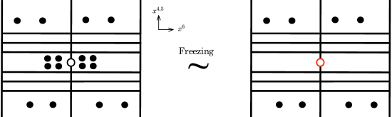
Figure 12: $\mathsf{LEFT}$: A IIA brane configuration for 4d SU($N$)+1$\textbf{AS}+(N+2)\mathbf{F}$ ($N=6$ in this case). $\mathsf{RIGHT}$: A brane configuration for 4d SU($N$)+1$\textbf{Sym}+(N-2)\mathbf{F}$. Here, (color) D4 branes are extended along the $x^{6}$-direction, NS5-branes are extended along the $x^{4,5}$-directions, and (flavor) D6-branes ($x^{7,8,9}$) are denoted by black dots. Also, an O6^--plane is denoted by a black circle and an O6⁺-plane is by a red circle.

Similar to the construction of 5d gauge theories with (anti-)symmetric hypermultiplet in IIB 5-brane web diagrams, 4d SU$(N)$ gauge theories can be constructed from IIA brane setup with NS5-, D4-, and D6-branes/O6-planes, which is a T-dual of IIB brane configuration. More precisely, SU($N$) gauge theories with $N_{f}$ fundamental hypermultiplets are represented by $N$ D4-branes stretched between two NS5-branes, accompanied by $N_{f}$ D6-branes to account for the fundamental hypermultiplets. When one (anti-)symmetric hypermultiplet is introduced, the corresponding brane setup requires an O6^±-plane, respectively. This setup is illustrated in figure 12, where the brane arrangement is shown in the covering space, highlighting the D4/D6-branes mirrored by an O6-plane. The freezing here is the process in (52), $\textrm{O6}^{-}+4\textrm{D6}|_{\textrm{fixed}}\sim\textrm{O6}^{+}.$ One then clearly sees that if the middle NS5-brane is Higgsed away, then the resulting brane configuration becomes that for Sp/SO gauge theories with only fundamental hypermultiplets. Analogous to the case of the IIB brane configuration discussed earlier, the same kind of Higgsing reducing ranks of gauge and flavor groups by two is naturally realized on this IIA brane configuration as depicted in figure 13.

The process of unfreezing in the IIA brane setup is also evident. In figure 14, we illustrate a brane configuration for SU$(10)+1\textbf{Sym}+8\mathbf{F}$ with an O6⁺-plane for $1\textbf{Sym}$. Through unfreezing, we utilize $\textrm{O6}^{+}\sim\textrm{O6}^{-}+4\textrm{D6}|_{\textrm{fixed}}$, with the four D6 branes highlighted in red. At the same time, Higgsing is applied to eight color D4-branes arranged alongside eight D6-branes, subsequently relocated in the $x^{7,8,9}$ direction. Following the Hanany-Witten transitions, one finds that the resulting configuration is a IIA brane configuration SU$(2)+1\textbf{AS}+4\mathbf{F}$, as shown on the right of the figure 14, where red dots represent free hypermultiplets.

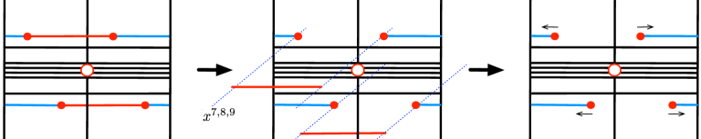
Figure 13: Higgsing with $\textbf{AS}/\textbf{Sym}$ in IIA brane setup: $\operatorname{SU}(N+2)+1\textbf{AS}/\textbf{Sym}+2\mathbf{F}\to\operatorname{SU}(N)+1\textbf{AS}/\textbf{Sym}$. In the last figure, Hanany-Witten transitions are performed to two D6 branes along the direction of the arrows.

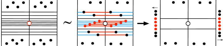
Figure 14: Unfreezings for on IIA brane setup, suggesting $\operatorname{SU}(N+8)+1\textbf{Sym}+(N+6)\mathbf{F}\to\operatorname{SU}(N)+1\textbf{AS}+(N+2)\mathbf{F}$. Here, $N=2$. LEFT: a brane configuration for $\operatorname{SU}(10)+1\textbf{Sym}+8\mathbf{F}$ with a red circle denoting an O6⁺. MIDDLE: an $\textrm{O6}^{+}\sim\textrm{O6}^{-}+$4D6 (unfreezing) and color D4-branes are align with D6-branes to be Higgsed. RIGHT: 8 D6-branes become free hypermultiplets by Hanany-Witten moves. The brane setup describes $\operatorname{SU}(2)+1\textbf{AS}+4\mathbf{F}$

Although the brane configuration illustrated in figure 14 suggests the relation between $\operatorname{SU}(N+8)+1\textbf{Sym}+(N+6)\mathbf{F}$ and $\operatorname{SU}(N)+1\textbf{AS}+(N+2)\mathbf{F}$, capturing this relation within the complete BPS spectrum in 4d is far from straightforward. Our analysis reveals that only a select few BPS observables truly reflect this relation as depicted by the brane setup. The Schur index stands out as one such observable. We will now delve into a detailed demonstration of how the unfreezing process manifests at the level of the Schur index.

Schur Index.

Based on the discussion of the Schur limit of the superconformal index earlier, we find that the Schur index for $\operatorname{SU}({N+8})+1\textbf{AS}+({N+10})\mathbf{F}$ can be expressed as follows:

$${I}^{\operatorname{SU}(N+8)+1\textbf{AS}+(N+10)\textbf{F}}_{\textrm{Schur}}= \oint_{\mathrm{T}^{N+7}}\frac{d\boldsymbol{z}}{2\pi i\boldsymbol{z}}{\mathcal{I}}^{\operatorname{SU}(N+8)+1\textbf{AS}+(N+10)\textbf{F}}_{\textrm{Schur}}$$ (101)

$$= \frac{(\mathfrak{q};\mathfrak{q})^{2(N+7)}}{(N+8)!}\oint_{\mathrm{T}^{N+7}}\frac{d\boldsymbol{z}}{2\pi i\boldsymbol{z}}\prod_{i=1}^{N+8}\prod_{j>i}\frac{\theta((z_{j}/z_{i})^{\pm})}{\theta(z_{i}z_{j}\mathfrak{m}\sqrt{\mathfrak{q}})}\prod_{k=1}^{N+10}\frac{1}{\theta(z_{i}\mathfrak{m}_{k}\sqrt{\mathfrak{q}})}~{}.$$

where $\mathfrak{m}$ is U(1) flavor fugacity of one antisymmetric hypermultiplet while $\mathfrak{m}_{k}$ are the $\operatorname{U}(N+10)$ flavor fugacities for the fundamental hypermultiplets.

In this setup, two Higgs branch operators acquire the vacuum expectation values (VEVs), which Higgses the gauge group by rank two:

$$\mathrm{SU}(N+2)+1\mathbf{AS}+(N+4)\mathbf{F}\ \xrightarrow{\textrm{Higgsing}}\ \mathrm{SU}(N)+1\mathbf{AS}+(N+2)\mathbf{F}~{}.$$ (102)

The Higgsing procedure can be seen at the level of the superconformal index Gaiotto:2012xa as follows. To move two D6 branes on a D4-brane, we tune the flavor fugacities $\mathfrak{m}_{N+9}=\frac{\mathfrak{m}}{\mathfrak{m}_{N+10}\sqrt{\mathfrak{q}}}$, and take residues at the particular values of the gauge fugacities

$$\Big{[}(N+8)(N+7)(\mathfrak{q};\mathfrak{q})^{2}\prod_{i=1}^{N+8}\theta(\mathfrak{m}_{N+10}/\mathfrak{m}_{i})\theta(\mathfrak{m}_{i}\mathfrak{m}_{N+10}\sqrt{\mathfrak{q}}/\mathfrak{m})\Big{]}^{-1}\mathcal{I}^{\operatorname{SU}(N+6)+1\textbf{AS}+(N+8)\textbf{F}}_{\textrm{Schur}}\\ =\Res^{\prime}_{z_{N+7}=\frac{\mathfrak{m}_{N+10}}{\mathfrak{m}}}\Res_{z_{N+8}=\frac{1}{\mathfrak{m}_{N+10}\sqrt{\mathfrak{q}}}}\mathcal{I}^{\operatorname{SU}(N+8)+1\textbf{AS}+(N+10)\textbf{F}}_{\textrm{Schur}}(\mathfrak{m}_{N+9}=\frac{\mathfrak{m}}{\mathfrak{m}_{N+10}\sqrt{\mathfrak{q}}})~{}.$$ (103)

Here, $\Res^{\prime}$ indicates that we remove the divergent zero modes by hand, which are typically present in the Higgsing process, when taking the residue. As illustrated on the left side of figure 15, by employing this procedure four times, we can reduce the gauge rank by eight through the appropriate assignment of VEVs to eight hypermultiplets.

Now let us see the freezing effect (52) at the level of the Schur index. To fix the position of four D6-branes near the O6^--plane, we set the flavor fugacities in the Schur index (101) as

$$\mathfrak{m}_{N+j}=\pm\mathfrak{m}^{\frac{1}{2}}\mathfrak{q}^{\pm\frac{1}{4}}~{},$$ (104)

where $j$ ranges from 7 to 10, and here we take all possible sign combinations. With this specialization, it reduces to the Schur index of $\operatorname{SU}(N+8)$ with one symmetric and $(N+6)$ fundamental hypermultiplets

$$\mathcal{I}^{\mathrm{SU}({N+8})+1\textbf{AS}+({N+10})\textbf{F}}_{\textrm{Schur}}\ \xrightarrow[\eqref{SCI-flavor-SU}]{\textrm{Freezing}}\ \mathcal{I}^{\mathrm{SU}({N+8})+1\textbf{Sym}+({N+6})\textbf{F}}_{\textrm{Schur}}~{},$$ (105)

where

$${I}^{\operatorname{SU}(N+8)+1\textbf{Sym}+(N+6)\textbf{F}}_{\textrm{Schur}}\\ =\frac{(\mathfrak{q};\mathfrak{q})^{2(N+7)}}{(N+8)!}\oint_{\mathrm{T}^{N+7}}\frac{d\boldsymbol{z}}{2\pi i\boldsymbol{z}}\prod_{i=1}^{N+8}\frac{1}{\theta(z_{i}^{2}\mathfrak{m}\sqrt{\mathfrak{q}})}\prod_{j>i}\frac{\theta((z_{j}/z_{i})^{\pm})}{\theta(z_{i}z_{j}\mathfrak{m}\sqrt{\mathfrak{q}})}\prod_{k=1}^{N+6}\frac{1}{\theta(z_{i}\mathfrak{m}_{k}\sqrt{\mathfrak{q}})}~{}.$$ (106)

To transition from the Schur index of $\operatorname{SU}(N+8)+1\textbf{Sym}+(N+6)\textbf{F}$ to $\operatorname{SU}(N)+1\textbf{AS}+(N+2)\textbf{F}$, we position an additional four D6-branes close to the O6^--plane. This is achieved by adjusting four flavor fugacities as follows:

$$\mathfrak{m}_{N+j}=\pm\mathfrak{m}^{-\frac{1}{2}}\mathfrak{q}^{\pm\frac{1}{4}}~{},$$ (107)

where $j$ ranges from 3 to 6, and we take all possible sign combinations here. Then, to implement the unfreezing, we bring eight color D4-branes near the O6^--plane. This is done by taking residues in the integrand of the Schur index for $\mathrm{SU}({N+8})+1\textbf{Sym}+({N+6})\textbf{F}$ at

$$z_{N+j}=\pm\mathfrak{m}^{\pm\frac{1}{2}}\mathfrak{q}^{\pm\frac{1}{4}}~{},\qquad(j=1\ldots,8)$$ (108)

where we remove the divergent zero modes appropriately. Consequently, we obtain the integrand of the Schur index for $\mathrm{SU}({N})+1\textbf{AS}+({N+2})\textbf{F}$ up to some factor:

$$\mathcal{I}^{\mathrm{SU}({N+8})+1\textbf{Sym}+({N+6})\textbf{F}}_{\textrm{Schur}}(\mathfrak{m}_{N+j}=\pm\mathfrak{m}^{-\frac{1}{2}}\mathfrak{q}^{\pm\frac{1}{4}})\ \xrightarrow[\eqref{poles}]{\textrm{Unfreezing}}\ \mathcal{I}^{\mathrm{SU}({N})+1\textbf{AS}+({N+2})\textbf{F}}_{\textrm{Schur}}~{}.$$ (109)

The entire procedure is illustrated in the left of figure 15.

Comment on the full superconformal indices:

Unlike the Schur index, when we extend our analysis to the full superconformal index with $\mathfrak{p},\mathfrak{q},\mathfrak{t}$, we find that no specific flavor fugacities provide the identity for the SCFTs involving the antisymmetric hypermultiplet and the one with the symmetric hypermultiplet. Moreover, while the Macdonald index Gadde:2011uv receives the same contributions from Higgs branch operators as the Schur index does, these theories cannot be related by the identities of the Macdonald indices. Specifically, the fugacity $\mathfrak{t}$ distinguishes these theories. It is desirable to discern why this overlap appears exclusively at the Schur index level.

Figure 15: Freezing, unfreezing and Higssing procedures for Schur indices. $\mathsf{LEFT}$: The Schur index of ${\mathrm{SU}({N+8})+1\textbf{AS}+({N+10})\textbf{F}}$, after the freezing process as in (104), is equal to that of ${\mathrm{SU}({N+8})+1\textbf{Sym}+({N+6})\textbf{F}}$. Furthermore, applying the unfreezing as in (107) and (108) identifies the Schur index of ${\mathrm{SU}({N+8})+1\textbf{Sym}+({N+6})\textbf{F}}$ with that of ${\mathrm{SU}({N})+1\textbf{AS}+({N+2})\textbf{F}}$, up to a factor.
$\mathsf{RIGHT}$: The Schur index for $\mathrm{Sp}(N+4)+(2N+10)\mathbf{F}$, following the freezing process as described in (113), matches the Schur index for $\mathrm{Sp}(N)+(2N+2)\mathbf{F}$. Moreover, by implementing the unfreezing processes, as detailed in (116) and (117), we can equate the Schur index of $\mathrm{Sp}(N)+(2N+2)\mathbf{F}$ to that of $\mathrm{SO}(2N+8)+(2N+6)\mathbf{F}$, up to a factor.

Sp($N$) and SO($2N$) gauge theories

We will now compare the Schur indices between the superconformal QCD of $\operatorname{Sp}(N)$ and $\operatorname{SO}(2N)$. For $\operatorname{Sp}(N)$, the superconformal condition is achieved with $2N+2$ fundamental half-hypermultiplets while the $\operatorname{SO}(2N)$ group achieves this with $2N-2$ fundamental half-hypermultiplets. Hence, the Schur index for the superconformal QCD of $\operatorname{Sp}(N+4)$ is determined as follows:

$${I}^{\operatorname{Sp}({N+4})+({2N+10})\textbf{F}}_{\textrm{Schur}}=\frac{(\mathfrak{q};\mathfrak{q})^{2(N+4)}}{(N+4)!2^{N+4}}\oint_{\mathrm{T}^{N+4}}\frac{d\boldsymbol{z}}{2\pi i\boldsymbol{z}}\prod_{i=1}^{N+4}\theta(z_{i}^{\pm 2})\prod_{j>i}\theta(z_{j}^{\pm}z_{i}^{\pm})\prod_{k=1}^{2N+10}\frac{1}{\theta(z_{i}^{\pm}\mathfrak{m}_{k}\sqrt{\mathfrak{q}})}~{}.$$ (110)

Let us Higgs the gauge group by rank one via the Hanany-Witten process after placing two D6-branes onto a D4-branes:

$$\operatorname{Sp}(N+4)+({2N+10})\textbf{F}\ \xrightarrow{\textrm{Higgsing}}\ \operatorname{Sp}(N+3)+({2N+8})\textbf{F}~{}.$$ (111)

Regarding the Schur index, we equate the flavor fugacities $\mathfrak{m}_{2N+10}$ and $\mathfrak{m}_{2N+9}$, and set the gauge fugacity to $z_{N+4}=\mathfrak{m}_{2N+9}\mathfrak{q}^{1/2}$:

$$\Big{[}2(N+4)(\mathfrak{q};\mathfrak{q})^{2}\prod_{i=1}^{2N+8}\theta(\mathfrak{m}_{2N+9}^{\pm}/\mathfrak{m}_{i})\Big{]}^{-1}{\mathcal{I}}^{\operatorname{Sp}(N+3)+({2N+8})\textbf{F}}_{\textrm{Schur}}\\ =\Res^{\prime}_{z_{N+4}=\mathfrak{m}_{2N+9}\mathfrak{q}^{1/2}}{\mathcal{I}}^{\operatorname{Sp}(N+4)+({2N+10})\textbf{F}}_{\textrm{Schur}}(\mathfrak{m}_{2N+10}=\mathfrak{m}_{2N+9})$$ (112)

where $\Res^{\prime}$ implies the exclusion of the divergent zero modes when taking residues. Sequentially applying this Higgsing process four times ultimately leads to the $\operatorname{Sp}(N)+(2N+2)\textbf{F}$ theory.

The freezing effect from (52) can be seen at the level of the Schur index. To set the positions of four D6-branes close to the O6^--plane, we specialize the four flavor fugacities in the Schur index (110) as follows:

$$\mathfrak{m}_{2N+6+j}=\pm 1,\pm\mathfrak{q}^{\frac{1}{2}}~{},$$ (113)

it reduces to the Schur index of the ${\operatorname{SO}(2N+8)+({2N+6})\textbf{F}}$ theory up to a factor of 2:

$$\mathcal{I}^{\operatorname{Sp}({N+4})+({2N+10})\textbf{F}}_{\textrm{Schur}}\ \xrightarrow[\eqref{SCI-flavor-SpSO}]{\textrm{Freezing}}\ \mathcal{I}^{\operatorname{SO}(2N+8)+({2N+6})\textbf{F}}_{\textrm{Schur}}~{},$$ (114)

where

$$\frac{1}{2}{I}^{\operatorname{SO}(2N+8)}_{\textrm{Schur}}=\frac{(\mathfrak{q};\mathfrak{q})^{2(N+4)}}{(N+4)!2^{N+4}}\oint_{\mathrm{T}^{N}}\frac{d\boldsymbol{z}}{2\pi i\boldsymbol{z}}\prod_{i=1}^{N+4}\prod_{j>i}\theta(z_{j}^{\pm}z_{i}^{\pm})\prod_{k=1}^{2N+6}\frac{1}{\theta(z_{i}^{\pm}\mathfrak{m}_{k}\sqrt{\mathfrak{q}})}~{}.$$ (115)

To transition from the Schur index of $\mathrm{SO}(2N+8)+(2N+6)\mathbf{F}$ to $\mathrm{Sp}(N)+(2N+2)\mathbf{F}$, we relocate an additional four D6-branes close to the $\mathrm{O}6^{-}$-plane, and Higgs four D4-branes out. This relocation is achieved by setting four flavor fugacities as follows:

$$\mathfrak{m}_{2N+2+j}=\pm 1,\pm\mathfrak{q}^{\frac{1}{2}}~{},$$ (116)

where $j=1,\ldots,4$. Subsequently, we take residues in the Schur index formula of $\mathrm{SO}(2N+8)+(2N+6)\mathbf{F}$ at

$$z_{N+j}=\pm 1,\pm\mathfrak{q}^{\frac{1}{2}}~{},\qquad(j=1,\ldots,4)$$ (117)

where we appropriately remove the divergent zero modes in the denominator. Consequently, we obtain the integrand of the Schur index for $\mathrm{Sp}(N)+(2N+2)\mathbf{F}$ up to an unimportant factor:

$$\mathcal{I}^{\mathrm{SO}(2N+8)+(2N+6)\mathbf{F}}_{\textrm{Schur}}(\mathfrak{m}_{2N+2+j}=\pm 1,\pm\mathfrak{q}^{\frac{1}{2}})\ \xrightarrow[\eqref{poles2}]{\textrm{Unfreezing}}\ \mathcal{I}^{\mathrm{Sp}({N})+({2N+2})\textbf{F}}_{\textrm{Schur}}~{}.$$ (118)

The whole relationship is depicted in the right of figure 15.

As noted earlier, the relation holds only at the Schur indices. We emphasize that no specific tuning of flavor and gauge fugacities can extend this relation to encompass the full superconformal index involving $\mathfrak{p},\mathfrak{q},\mathfrak{t}$, or its various other limits.

3.2 3d $\mathcal{N}=4$ sphere partition functions

In the context of 3d setups, the brane configurations for 3d $\mathcal{N}=4$ theories are closely related to those used for 4d $\mathcal{N}=2$ gauge theories. For example, as depicted in figure 12 with O6-planes and D6-branes, the concept of freezing can be adapted to 3d by substituting O6-planes with O5-planes and D6-branes with D5-branes, as illustrated by

$$\mathrm{O}5^{-}+2\,\textrm{D5}\Big{|}_{\textrm{fixed}}~{}\sim~{}\mathrm{O}5^{+}~{}.$$ (119)

A notable distinction is the extension of NS5-branes along the $x^{4,5,6}$-directions in 3d configurations. Thus, we will now turn our attention to the sphere partition function, which effectively represents the concept of freezing in 3d. Given the similarity of this procedure to those previously described, we will provide a concise overview here. In this setting, the (un)freezing can be captured by the three-sphere partition function Kapustin:2009kz . Since the procedure is very similar to the previous cases, our discussion here will be succinct for simplicity.

U($N$) gauge theories with (anti-)symmetric hypermultiplet

Freezing

An $S^{3}$ partition function is evaluated by supersymmetric localization in the pioneering work Kapustin:2009kz . The $S^{3}$ partition function for $\operatorname{U}(N)$ gauge group with one antisymmetric and $(N_{f}+2)$ fundamental hypermultiplets is

$$Z_{S^{3}}^{\operatorname{U}(N)+1\textbf{AS}+(N_{f}+2)\mathbf{F}}(m)=\frac{1}{N!}\int[d\mathrm{s}]\prod_{i=1}^{N}\frac{e^{2\pi i\xi s_{i}}\prod_{j>i}\operatorname{sh}^{2}2\pi(s_{i}-s_{j})}{\prod_{j>i}\operatorname{ch}2\pi(s_{i}+s_{j}-m)\prod_{k=1}^{N_{f}+2}\operatorname{ch}2\pi(s_{i}-m_{k})}~{},$$ (120)

where $\xi$ is the Fayet-Iliopoulos term, $m$ is the mass of the antisymmetric and $m_{k}$ are those of the fundamentals. To incorporate the effect of freezing two D5-branes with an O5^--plane (119), we specialize two mass parameters as

$$m_{N_{f}+1}=\frac{m}{2}-\frac{i}{4}~{},\quad m_{N_{f}+2}=\frac{m}{2}+\frac{i}{4}$$ (121)

in the aforementioned partition function. This adjustment yields the partition function for $\operatorname{U}(N)$ gauge group with one symmetric and $N_{f}$ fundamental hypermultiplets (up to a factor of $i$):

$$Z_{S^{3}}^{\operatorname{U}(N)+1\textbf{AS}+(N_{f}+2)}\ \xrightarrow[\eqref{S3-freezing}]{\textrm{Freezing}}\ Z_{S^{3}}^{\operatorname{U}(N)+1\textbf{Sym}+N_{f}\mathbf{F}}~{}.$$ (122)

where

$$Z_{S^{3}}^{\operatorname{U}(N)+1\textbf{Sym}+N_{f}\mathbf{F}}(m)\\ =\frac{1}{N!}\int[d\mathrm{s}]\prod_{i=1}^{N}\frac{e^{2\pi i\xi s_{i}}\prod_{j>i}\operatorname{sh}^{2}2\pi(s_{i}-s_{j})}{\operatorname{ch}2\pi(2s_{i}-m)\prod_{j>i}\operatorname{ch}2\pi(s_{i}+s_{j}-m)\prod_{k=1}^{N_{f}}\operatorname{ch}2\pi(s_{i}-m_{k})}~{}.$$ (123)

Here we use the addition formula

$$\operatorname{sh}2\pi(2s)=\operatorname{ch}2\pi(s)\operatorname{sh}2\pi(s)~{}.$$ (124)

Unfreezing

Now let us turn to the process of unfreezing. To separate the two D5-branes used in the freezing process (119), we move two color D3-branes to the position of the D5-branes. Subsequently, through Higgsing and the Hanany-Witten transition, the D5-branes are moved away. To apply this change to the $S^{3}$ partition function, we can take the residues at $\frac{m}{2}\pm\frac{i}{4}$

$$\mathcal{Z}_{S^{3}}^{\operatorname{U}(N-2)+1\textbf{AS}+N_{f}\mathbf{F}}(m)$$ (125)

$$= \Big{[}2N(N-1)ie^{-2\pi im\xi}\prod_{k=1}^{N_{f}}\operatorname{ch}(m-2m_{k})\Big{]}\ \Res_{z_{N}=\frac{m}{2}-\frac{i}{4}}\Res_{z_{N-1}=\frac{m}{2}+\frac{i}{4}}\mathcal{Z}_{S^{3}}^{\operatorname{U}(N)+1\textbf{Sym}+N_{f}\mathbf{F}}(m)~{}.$$

In this way, we can see the unfreezing at the level of the $S^{3}$ partition functions

$$\mathcal{Z}_{S^{3}}^{\operatorname{U}(N)+1\textbf{Sym}+N_{f}\mathbf{F}}\ \xrightarrow{\textrm{unfreezing}}\ \mathcal{Z}_{S^{3}}^{\operatorname{U}(N-2)+1\textbf{AS}+N_{f}\mathbf{F}}~{}.$$ (126)

Sp($N$) and SO($2N$) gauge theories

Freezing

The $S^{3}$ partition function of 3d $\mathcal{N}=4$ SQCD with a simple gauge group $G$ and $N_{f}$ half-hypermultiplets carrying representations $w$ can be computed by

$$Z_{S^{3}}^{G+N_{f}\mathbf{F}}=\frac{1}{|W_{G}|}\lim_{\xi\to 0}\int[d\mathrm{s}]\frac{e^{2\pi i\xi\sum_{i=1}^{\textrm{rk}G}s_{i}}\prod_{\alpha\in\Delta}\operatorname{sh}2\pi(\alpha\cdot s)}{\prod_{j=1}^{N_{h}}\prod_{w\in\mathcal{R}}\operatorname{ch}2\pi(w\cdot s-m_{j})}\ ,$$ (127)

where $\Delta$ and $\mathcal{R}$ refer to, respectively, the root system of $G$ and the weights of the representation associated with the hypermultiplet. Although a simple gauge group does not admit the Fayet-Ilioupolous term, we introduce a regulator $\xi$ and take the limit $\xi\to 0$ to calculate the $S^{3}$ partition functions Benvenuti:2011ga .

The $S^{3}$ partition function of $\operatorname{Sp}(N)$ SQCD with $(N_{f}+2)$ fundamental hypermultiplets is given by

$$Z_{S^{3}}^{\operatorname{Sp}(N)+(N_{f}+2)\mathbf{F}}(m)= \frac{1}{N!2^{N}}\lim_{\xi\to 0}\int[d\mathrm{s}]\prod_{i=1}^{N}\frac{e^{2\pi i\xi s_{i}}\operatorname{sh}^{2}2\pi(2s_{i})\prod_{j>i}\operatorname{sh}^{2}2\pi(s_{i}\pm s_{j})}{\prod_{j=1}^{N_{f}+2}\operatorname{ch}2\pi(\pm s_{i}-m_{j})}$$ (128)

$$= \sum_{I\in C_{N}^{N_{f}+2}}\prod_{j=1}^{N}\frac{m_{I_{j}}\operatorname{sh}2\pi(2m_{I_{j}})}{\prod_{\ell\not\in I}\operatorname{sh}2\pi(m_{\ell}\pm m_{I_{j}})}~{},$$ (129)

where $I$ denotes a subset of $N$ distinct integers selected from $\{1,\ldots,N_{f}+2\}$, representing all possible combinations $C_{N}^{N_{f}+2}$. The transition from the integral expression in the first line to the sum in the second line is facilitated by isolating the poles at

$$s_{j}=\pm m_{I_{j}}+i\frac{2k_{j}+1}{2},\quad k_{j}\in\mathbb{Z}_{\geq 0}$$

and considering the symmetries of permutations $S_{N}$ of the set $I$. The limit $\xi\rightarrow 0$ is then applied using L’Hospital’s rule to derive the summation form as shown in the second line (Nawata:2021nse, , appendix D).

Now to perform the freezing (119), we specialize the two mass parameters in the $\operatorname{Sp}(N)$ partition function (128) as

$$m_{N_{f}+1}=0~{},\qquad m_{N_{f}+2}=\frac{i}{2}~{}.$$ (130)

This adjustment brings the partition function into the one for $\operatorname{SO}(2N)$ SQCD with $N_{f}$ fundamental hypermultiplets up to a factor of 2:

$$Z_{S^{3}}^{\operatorname{SO}(2N)+N_{f}\mathbf{F}}(m)= \,\frac{1}{N!2^{N-1}}\lim_{\xi\to 0}\int[d\mathrm{s}]\prod_{i=1}^{N}\frac{e^{2\pi i\xi s_{i}}\prod_{j>i}\operatorname{sh}^{2}2\pi(s_{i}\pm s_{j})}{\prod_{j=1}^{N_{f}}\operatorname{ch}2\pi(\pm s_{i}-m_{j})}$$ (131)

$$= \ 2\sum_{I\in C_{N}^{N_{f}}}\prod_{j=1}^{N}\frac{m_{I_{j}}}{\operatorname{sh}2\pi(2m_{I_{j}})\prod_{\ell\notin I}\operatorname{sh}2\pi(m_{\ell}\pm m_{I_{j}})}~{}.$$ (132)

This freezing can be verified directly in the integrands and also through the integrated expressions:

$$Z_{S^{3}}^{\operatorname{Sp}(N)+(N_{f}+2)\mathbf{F}}\ \xrightarrow[\eqref{S3-freezing2}]{\textrm{Freezing}}\ Z_{S^{3}}^{\operatorname{SO}(2N)+N_{f}\mathbf{F}}~{}.$$ (133)

Unfreezing

The subsequent steps are also analogous. To undo the freezing process described in (119), we introduce two additional D5-branes alongside two color branes in the vicinity of the $\mathrm{O}5$-plane. This is followed by the processes of Higgsing and Hanany-Witten transition. For the $S^{3}$ partition functions, we then adjust the mass parameters to

$$m_{N_{f}}=0~{},\quad m_{N_{f}-1}=\frac{i}{2}~{},$$ (134)

and fine-tune the gauge fugacities to

$$z_{N}=0~{},\quad z_{N-1}=\frac{i}{2}~{}.$$ (135)

Through these adjustments, the unfreezing processes become evident at the level of the $S^{3}$ partition functions, leading to the transformation

$$\mathcal{Z}_{S^{3}}^{\operatorname{SO}(2N)+N_{f}\mathbf{F}}\ \xrightarrow[(\ref{S3-mass2},\ref{S3-gauge2})]{\textrm{unfreezing}}\ \mathcal{Z}_{S^{3}}^{\operatorname{Sp}(N-2)+(N_{f}-2)\mathbf{F}}.$$ (136)

Comments on other partition functions

In 3d, other exact partition functions are available. The 3d $\mathcal{N}=4$ superconformal index Razamat:2014pta can be understood as a partition function on $S^{1}\times S^{2}$ with appropriate background fields introduced. However, there is no fine-tuning of the flavor symmetries to match the superconformal indices of the two theories compared above. Since 3d $\mathcal{N}=4$ theories are endowed with $\operatorname{SU}(2)_{H}\times\operatorname{SU}(2)_{C}$ $R$-symmetry, performing topological twists Rozansky:1996bq , one can also consider a twisted partition function on a general three-manifold. Notably, A-twisted and B-twisted indices on a Riemann surface, $S^{1}\times\Sigma_{g}$, have been studied in (Closset:2016arn, , §6) where A-twist (resp. B-twist) corresponds to a topological twist with $\operatorname{SU}(2)_{H}$ (resp. $\operatorname{SU}(2)_{C}$). Specifically, A-twisted and B-twisted indices on $S^{1}\times S^{2}$ provide the Hilbert series of the Coulomb and Higgs branch of the 3d $\mathcal{N}=4$ theory, respectively. Once more, the twisted indices show no specialization in flavor fugacities that leads the indices of the two compared theories to be equal. This particularly indicates that the two theories have distinct Coulomb and Higgs branch moduli spaces. This distinction demonstrates that the two theories are not dual to each other, even when considering specific mass parameters and flavor fugacities. Hence, the correspondence in the $S^{3}$ partition function remains observational.

4 Conclusion

In this study, we introduce a fascinating link between the BPS partition functions for a family of supersymmetric gauge theories equipped with eight supercharges. These theories are characterized by brane configurations that incorporate an O$p^{+}$-plane across dimensions $d=5,4,3$, with $p=d+2$.

In particular, in five dimensions, we show that the partition functions tied to an O7⁺-plane emerge from configurations with an O7^--plane and eight D7-branes through a process we term “freezing.” This process is applicable to theories such as $\operatorname{SU}(N)_{\kappa}+1\textbf{Sym}+N_{f}\mathbf{F}\leftarrow\operatorname{SU}(N)_{\kappa}+1\textbf{AS}+(N_{f}+8)\mathbf{F}$ and $\operatorname{SO}(2N)+N_{f}\mathbf{F}\leftarrow\operatorname{Sp}(N)+(N_{f}+8)\mathbf{F}$, respectively for $N\geq 2$ and $N_{f}$ up to the flavor limit of 5d Kaluza-Klein (KK) theories. We find that their refined instanton partition functions match when we apply mass specializations to the hypermultiplets, a direct outcome of freezing. A notable example is the application of freezing to the 5d KK theory $\operatorname{SU}(2)+8\mathbf{F}$, commonly referred to as E-string theory on a circle. At the level of partition functions, this results in the KK theory $\operatorname{SU}(2)_{\theta}+1\mathbf{Adj}$, where $\theta=0$ aligns with the 6d M-string on a circle, and $\theta=\pi$ links to the 6d $A_{2}$ theory on a circle with a $\mathbb{Z}_{2}$ outer automorphism twist.

Furthermore, we identify a novel phenomenon where the BPS instanton spectrum jumps from one theory to another through “unfreezing,” a reversal of the freezing process, in 5d theories. Unfreezing necessitates precise adjustments of mass and Coulomb branch parameters, followed by successive Higgsings in the partition function calculation. This leads to the emergence of degenerate poles in the JK residue integrals, subsequently resulting in the appearance of multiplicity coefficients that facilitate shifts in the partition functions. We have concretely verified that $\operatorname{SU}(N+8)_{\kappa}+1\textbf{Sym}+8\mathbf{F}\dashrightarrow\operatorname{SU}(N)_{\kappa}+1\textbf{AS}$ and $\operatorname{SO}(2N+8)\dashrightarrow\operatorname{Sp}(N)$ for the unrefined case.

The processes of freezing and unfreezing can be applied to both 4d and 3d supersymmetric gauge theories. While the brane configurations in these dimensions may not be as visually intuitive as in the five-dimensional case, the charges associated with orientifold planes connect distinct theories. Specifically, in four dimensions, this relationship is represented by $\mathrm{O}6^{+}\sim\mathrm{O}6^{-}+4\mathrm{D}6$, and in three dimensions, by $\mathrm{O}5^{+}\sim\mathrm{O}5^{-}+2\mathrm{D}5$. We have found that, in these lower-dimensional theories, only certain physical observables agree under the processes of freezing and unfreezing. For example, under the freezing, the Schur index for a 4d $\mathcal{N}=2$ SU($N$) gauge theory with a symmetric hypermultiplet matches that of a theory with an antisymmetric hypermultiplet and $(N+2)$ fundamental hypermultiplets. Similarly, the relationship of these theories through unfreezing is depicted in figure 15. In three dimensions, the equivalence of $S^{3}$ partition functions between 3d $\mathcal{N}=4$ U($N$) gauge theories with symmetric and antisymmetric hypermultiplets, alongside two fundamental hypermultiplets, is explicitly verified. The $S^{3}$ partition functions for Sp/SO gauge theories have also been confirmed.

We remark that it is well-known that 5-brane webs for SO/Sp gauge theories can be constructed using an O5-plane instead of an O7-plane. For a single gauge group, naively a 5-brane web with an O7-plane is not much distinct from that with an O5-plane. For instance, SW curves obtained from 5-brane webs with an O7- and an O5-plane are equivalent Hayashi:2017btw ; Hayashi:2023boy . Hence, the freezing and unfreezing associated with an O5-plane can be also understood similarly. For instance, a freezing process with an O5-plane is depicted in figure 16 relating the 5d Sp($N)+8\mathbf{F}$ and the 5d SO($2N$) theory.

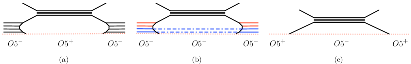
Figure 16: 5-brane webs with an O5-plane and freezing. (a) 5-brane web for $\operatorname{Sp}(N)+8\mathbf{F}$ theory. (b) Freezing: ${\rm O}5^{+}\sim{\rm O}5^{-}+2\mathbf{F}$ denoted by blue dashed lines. (c) Together with virtual Higgsings with blue “color” branes and flavor branes, the freezing takes place on O5^--plane with flavor D5-brane (in red), leading to an O5⁺-plane, which results in a 5-brane web for $\operatorname{SO}(2N)$ theory.

The study of the freezing and unfreezing in this paper raises interesting questions and several promising directions to consider. First of all, we observe that certain physical observables agree upon freezing though this agreement is not universal across all observables, as demonstrated in the 4d and 3d contexts. Given that freezing does not constitute a duality, discrepancies in observables are to be expected. Nonetheless, it is crucial to uncover any underlying principles that explain why specific observables match under freezing.

Moreover, we encounter the BPS jumping phenomenon during unfreezing. This behavior is anticipated to occur more generally when degenerate poles appear in the JK residue integrals upon varying chemical potentials. This suggests that observing BPS jumping through JK residue integrals becomes feasible when chemical potentials, serving as physical parameters, are adjustable. A systematic examination of the conditions leading to BPS jumping and the physical mechanisms driving this phenomenon would be essential next steps.

Expanding this analysis to other dimensions presents another compelling direction for research. While our attention has primarily been on 5d instanton partition functions, it would be interesting to extend the investigation to 6d elliptic genera and Little String Theory partition functions through the viewpoint of $\mathrm{O}8^{+}\sim\mathrm{O}8^{-}+16\mathrm{D}8$. Exploring a 2d extension, where freezing implies a relation $\mathrm{O}4^{+}\sim\mathrm{O}4^{-}+1\mathrm{D}4$, may offer another valuable perspective. Additionally, the study of the freezing in the context of string dualities such as T-duality invites further investigation.

Another aspect worth exploring is whether the process of (un)freezing can be applied to theories and configurations with less supersymmetry. Since the freezing process $\mathrm{O}p^{+}\sim\mathrm{O}p^{-}+2^{p-4}~{}\textrm{D}p$ can be implemented locally within brane configurations, it is feasible to decrease the amount of supersymmetry by altering global configurations or incorporating additional branes. Investigating the process of (un)freezing in more general brane setups would be also an interesting direction for future research.

Appendix A Notation and convention

In this appendix, we outline the specific notations and conventions employed throughout this paper.

First of all, throughout the paper, we denote the product (resp. sum) of all possible sign combinations for multiplicative (resp. additive) parameters in the following expressions:

$$f(\mathfrak{a}^{\pm}\mathfrak{b}^{\pm}) =f(\mathfrak{a}\mathfrak{b})f(\mathfrak{a}^{-1}\mathfrak{b})f(\mathfrak{a}\mathfrak{b}^{-1})f(\mathfrak{a}^{-1}\mathfrak{b}^{-1}),$$ (137)

$$g(\pm a\pm b) =g(a+b)g(-a+b)g(a-b)g(-a-b),$$

For mass or Coulomb branch specialization,

$$a=A(\pm\pi i)\quad\Leftrightarrow\quad a=A,~{}A+\pi i,~{}A-\pi i\ .$$ (138)

For various SU, Sp, and SO gauge theories, we frequently use the following concise notations for matter hypermultiplet representations:

• Fundamental representation: $\mathbf{F}$

• Antisymmetric representation: AS

• Symmetric representation: Sym

Young diagrams

:

A Young diagram $\lambda$ is defined by a non-increasing sequence of non-negative integers, $\lambda=(\lambda_{1}\geq\lambda_{2}\geq\ldots\geq\lambda_{\ell(\lambda)}>0)$. The length of a Young diagram, denoted by $\ell(\lambda)$, is the number of its non-zero rows. The total number of boxes in the Young diagram is denoted by

$$|\lambda|=\sum_{i=1}^{\ell(\lambda)}\lambda_{i}~{}.$$ (139)

The transpose of the Young diagram $\lambda$, denoted by $\lambda^{t}$, is obtained by reflecting $\lambda$ along its main diagonal. For a box $x=(i,j)\in\lambda$, where $i$ is the row index and $j$ is the column index, the arm length $A_{\lambda}(x)$ and the leg length $L_{\lambda}(x)$ are defined as

$$A_{\lambda}(x)=\lambda_{i}-j\qquad L_{\lambda}(x)=\lambda^{t}_{j}-i$$ (140)

We also denote that $\alpha(\lambda)$ is the number of rows with $\lambda_{i}\geq i$ while $\beta(\lambda)$ is the number of rows with $\lambda_{i}\geq i+1$:

$$\alpha(\lambda)=\max(i\mid\lambda_{i}\geq i)~{},\qquad\beta(\lambda)=\max(i\mid\lambda_{i}\geq i+1)~{}.$$ (141)

(See figure 17 for an example.)

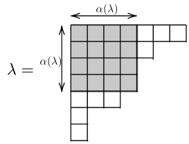
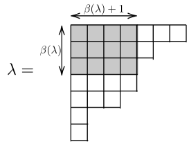
Figure 17: $\alpha(\lambda)$ is the number of rows with $\lambda_{i}\geq i$ while $\beta(\lambda)$ is the number of rows with $\lambda_{i}\geq i+1$. For $\lambda=(7,5,4,4,3,1,1)$, $\alpha(\lambda)=4$ and $\beta(\lambda)=3$.

For an expression of an instanton partition function, we often use the following notation of the $P$-tuple Young diagrams with $k$ a total number of boxes:

$$\vec{\lambda}=(\lambda^{(1)},\ldots,\lambda^{(P)})~{},$$

and

$$|\vec{\lambda}|:=\sum_{s=1}^{P}|\lambda^{(s)}|=k~{}.$$

Partition Functions

:

In our notation, the integrand of a partition function is denoted in calligraphic font, while the resultant partition function is represented in standard lettering. For example, a $k$-instanton partition function is expressed as

$$Z_{k}^{\mathcal{T}}=\oint_{\textrm{JK}}\prod_{I}\frac{d\phi_{I}}{2\pi i}~{}\mathcal{Z}^{\mathcal{T}}_{k}(\boldsymbol{\phi})\ ,$$ (142)

where $\mathcal{T}$ symbolizes the theory under consideration. An instanton partition function is defined on the $\Omega$-background Nekrasov:2002qd , and we use the standard notation $\epsilon_{1,2}$ to represent the $\Omega$-deformation parameters. We also introduce the notation $2\epsilon_{\pm}=\epsilon_{1}\pm\epsilon_{2}$, with the unrefined limit being defined as $\epsilon_{1}=-\epsilon_{2}=\hbar$ (therefore $\epsilon_{+}=0,~{}\epsilon_{-}=\hbar$) For the 5d instanton partition function, it is also helpful to introduce the notations

$$\operatorname{sh}(x):=e^{\frac{x}{2}}-e^{-\frac{x}{2}},\qquad\operatorname{ch}(x):=e^{\frac{x}{2}}+e^{-\frac{x}{2}}~{},$$ (143)

which satisfy the relation

$$\operatorname{ch}(x)=-i\operatorname{sh}(x+\pi i)~{},\qquad\operatorname{sh}(2x)=\operatorname{sh}(x)\operatorname{ch}(x)\ .$$ (144)

For a superconformal index, the integrand is also denoted in calligraphic type, and the index post-integration in standard lettering:

$$I^{\mathcal{T}}=\oint_{\mathrm{T}}\prod_{j}\frac{dz_{j}}{2\pi iz_{j}}~{}\mathcal{I}^{\mathcal{T}}(\boldsymbol{z}).$$ (145)

We use fraktur font for fugacities in the superconformal index. The integrand $\mathcal{I}$ is represented by the elliptic Gamma function, defined as

$$\Gamma(z;\mathfrak{p},\mathfrak{q})=\prod_{m,n=0}^{\infty}\frac{1-\mathfrak{p}^{m+1}\mathfrak{q}^{n+1}/z}{1-\mathfrak{p}^{m}\mathfrak{q}^{n}z}=\operatorname{PE}\bigg{[}\frac{z-\frac{\mathfrak{p}\mathfrak{q}}{z}}{(1-\mathfrak{q})(1-\mathfrak{p})}\bigg{]}.$$ (146)

The $\mathfrak{q}$-Pochhammer symbol is defined as

$$(x;\mathfrak{q}):=\prod_{i=0}^{\infty}(1-x\mathfrak{q}^{i})\ ,$$

and the theta function as

$$\theta(x;\mathfrak{q})=(x;\mathfrak{q})(\mathfrak{q}x^{-1};\mathfrak{q})\ .$$

Appendix B ADHM contour integrals

This appendix lists contributions to the instanton partition functions from various fields in 5d theories with classical gauge groups. Specifically, 5d supersymmetric theories on the $\Omega$-background effectively localize to supersymmetric quantum mechanics on instanton moduli spaces. These spaces are described by the Atiyah-Drinfeld-Hitchin-Manin (ADHM) construction Atiyah:1978ri for classical groups. Therefore, the contributions of various fields to the instanton partition functions are derived from the ADHM descriptions of these instanton moduli spaces and their associated bundles. For a more detailed explanation, we refer readers to Moore:1997dj ; Nekrasov:2002qd ; Nekrasov-Shadchin ; Shadchin:2005mx ; Kim:2012gu ; Hwang:2014uwa .

B.1 $\operatorname{SU}(N)$ gauge group

For SU($N$) gauge group, we list the contributions from hypermultiplets in the fundamental, (anti-)symmetric, and adjoint representations:

$$\mathcal{Z}_{\operatorname{SU}(N)_{\kappa},k}^{\textrm{vec}}= ~{}e^{\kappa\sum_{I=1}^{k}\phi_{I}}\frac{\prod_{I\neq J}\operatorname{sh}(\phi_{I}-\phi_{J})\cdot\prod_{I,J}\operatorname{sh}(2\epsilon_{+}-\phi_{I}+\phi_{J})}{\prod_{I,J}\operatorname{sh}(\epsilon_{1,2}+\phi_{I}-\phi_{J})\prod_{I=1}^{k}\prod_{s=1}^{N}\operatorname{sh}(\epsilon_{+}\pm(\phi_{I}-a_{s}))}$$ (147)

$$\mathcal{Z}_{\operatorname{SU}(N),k}^{N_{f}}(m_{l})= \prod_{l=1}^{N_{f}}\prod_{I=1}^{k}\operatorname{sh}(\phi_{I}+m_{l})$$ (148)

$$\mathcal{Z}_{\operatorname{SU}(N),k}^{\textrm{sym}}(m)= \prod_{I=1}^{k}\operatorname{sh}{(2\phi_{I}+m\pm\epsilon_{-})}\prod_{s=1}^{N}\operatorname{sh}{(\phi_{I}+a_{s}+m)}\prod_{I<J}^{k}\frac{\operatorname{sh}{(\phi_{I}+\phi_{J}+m\pm\epsilon_{-})}}{\operatorname{sh}{(-\epsilon_{+}\pm(\phi_{I}+\phi_{J}+m))}}$$ (149)

$$\mathcal{Z}_{\operatorname{SU}(N),k}^{\textrm{anti}}(m)= \prod_{I=1}^{k}\frac{\prod_{s=1}^{N}\operatorname{sh}{(\phi_{I}+a_{s}+m)}}{\operatorname{sh}{(-\epsilon_{+}\pm(2\phi_{I}+m))}}\prod_{I<J}^{k}\frac{\operatorname{sh}{(\phi_{I}+\phi_{J}+m\pm\epsilon_{-})}}{\operatorname{sh}{(-\epsilon_{+}\pm(\phi_{I}+\phi_{J}+m))}}$$ (150)

$$\mathcal{Z}_{\operatorname{SU}(N),k}^{\textrm{adj}}(m)= \prod_{I=1}^{k}\frac{\operatorname{sh}{(\epsilon_{-}\pm m)}\prod_{s=1}^{N}\operatorname{sh}{(m\pm(\phi_{I}-a_{s}))}}{\operatorname{sh}{(\epsilon_{+}\pm m)}}\prod_{I<J}^{k}\frac{\operatorname{sh}{(\epsilon_{-}\pm m\pm(\phi_{I}-\phi_{J}))}}{\operatorname{sh}{(\epsilon_{+}\pm m\pm(\phi_{I}-\phi_{J}))}}$$ (151)

B.2 $\operatorname{SO}(n)$ gauge group

In the case of the SO($n$) gauge group, the nature of contributions depends on whether $n$ is even or odd. We represent $n=2N+\chi$, where $n\equiv\chi$ mod 2. Then, we can write the contributions from hypermultiplets in the fundamental, adjoint (antisymmetric), and symmetric representations:

$$\mathcal{Z}_{\operatorname{SO}(n),k}^{\textrm{vec}}$$ (153)

$$= \frac{1}{2^{k}\,k!}\frac{\operatorname{sh}^{k}(2\epsilon_{+})}{\operatorname{sh}^{k}(\epsilon_{1,2})}\prod_{I=1}^{k}\frac{\operatorname{sh}(2\epsilon_{+}\pm 2\phi_{I})\,\operatorname{sh}(\pm 2\phi_{I})}{\operatorname{sh}^{\chi}(\epsilon_{+}\pm\phi_{I})\prod_{s=1}^{N}\operatorname{sh}(\epsilon_{+}\pm\phi_{I}\pm a_{s})}\prod_{I<J}\frac{\operatorname{sh}(2\epsilon_{+}\pm\phi_{I}\pm\phi_{J})\,\operatorname{sh}(\pm\phi_{I}\pm\phi_{J})}{\operatorname{sh}(\epsilon_{1,2}\pm\phi_{I}\pm\phi_{J})}$$ (154)

$$\mathcal{Z}_{\operatorname{SO}(n),k}^{N_{f}}(m_{l})=\prod_{l=1}^{N_{f}}\prod_{I=1}^{k}\operatorname{sh}\left(\pm\phi_{I}+m_{l}\right)$$ (155)

$$\mathcal{Z}_{\operatorname{SO}(n),k}^{\textrm{adj}}(m)=\prod_{I=1}^{k}\frac{\operatorname{sh}{(\pm m-\epsilon_{-})}\operatorname{sh}^{\chi}(m\pm\phi_{I})\prod_{s=1}^{\lfloor\frac{n}{2}\rfloor}\operatorname{sh}{(\pm\phi_{I}\pm a_{s}+m)}}{\operatorname{sh}{(\pm m-\epsilon_{+})}\operatorname{sh}{(\pm 2\phi_{I}\pm m-\epsilon_{+})}}\prod_{I<J}^{k}\frac{\operatorname{sh}{(\pm\phi_{I}\pm\phi_{J}\pm m-\epsilon_{-})}}{\operatorname{sh}{(\pm\phi_{I}\pm\phi_{J}\pm m-\epsilon_{+})}}$$ (156)

$$\mathcal{Z}_{\operatorname{SO}(n),k}^{\textrm{sym}}(m)=\prod_{I=1}^{k}\frac{\operatorname{sh}{(\pm m-\epsilon_{-})}\operatorname{sh}{(\pm 2\phi_{I}\pm m-\epsilon_{-})}\operatorname{sh}^{\chi}(m\pm\phi_{I})\prod_{s=1}^{\lfloor\frac{n}{2}\rfloor}\operatorname{sh}{(\pm\phi_{I}\pm a_{s}+m)}}{\operatorname{sh}{(\pm m-\epsilon_{+})}}$$ (157)

$$\quad\qquad\qquad\quad\cdot\prod_{I<J}^{k}\frac{\operatorname{sh}{(\pm\phi_{I}\pm\phi_{J}\pm m-\epsilon_{-})}}{\operatorname{sh}{(\pm\phi_{I}\pm\phi_{J}\pm m-\epsilon_{+})}}$$ (158)

B.3 $\operatorname{Sp}(N)$ gauge group

For $\operatorname{Sp}(N)$ gauge group, the instanton partition functions depend on the discrete $\theta$-angle in general. This is rooted in the topological property that $\pi_{4}(\operatorname{Sp}(N))=\mathbb{Z}_{2}$ Morrison:1996xf ; Douglas:1996xp . Such a property is manifested in the way supersymmetric quantum mechanics is described by the $\mathrm{O}(k)^{\pm}$ gauge group which has two disconnected components. Denoting these respective contributions as $Z^{\pm}_{k}$, a choice of taking the sum or difference of $Z^{\pm}_{k}$ corresponds to $\theta=0$ or $\theta=\pi$. Thus, the $k$-instanton partition function with trivial $\theta$-angle is given by

$$Z^{\theta=0}_{k}=\frac{Z^{+}_{k}+Z^{-}_{k}}{2},$$

whereas that with non-trivial $\mathbb{Z}_{2}$ element is given by

$$Z^{\theta=\pi}_{k}=(-1)^{k}\frac{Z^{+}_{k}-Z^{-}_{k}}{2}~{}.$$

Therefore, in the following, we enumerate contributions from both plus and minus sectors for hypermultiplets in the fundamental, adjoint (symmetric), antisymmetric representations.

Vector multiplet

$$\mathcal{Z}_{\operatorname{Sp}(N),k=2\ell+\chi}^{\textrm{vec},+}= \frac{1}{2^{\ell-1+\chi}\ell!}\left(\frac{1}{\operatorname{sh}{(\epsilon_{1,2})}\,\prod_{s=1}^{N}\operatorname{sh}{(\epsilon_{+}\pm a_{s})}}\cdot\prod_{I=1}^{\ell}\frac{\operatorname{sh}{(\pm\phi_{I})}\operatorname{sh}{(2\epsilon_{+}\pm\phi_{I})}}{\operatorname{sh}{(\epsilon_{1,2}\pm\phi_{I})}}\right)^{\chi}$$ (159)

$$\cdot\prod_{I=1}^{\ell}\frac{\operatorname{sh}{(2\epsilon_{+})}}{\operatorname{sh}{(\epsilon_{1,2})}\operatorname{sh}(\epsilon_{1,2}\pm 2\phi_{I})\,\prod_{s=1}^{N}\operatorname{sh}{(\epsilon_{+}\pm\phi_{I}\pm a_{s})}}\prod_{I<J}^{\ell}\frac{\operatorname{sh}(2\epsilon_{+}\pm\phi_{I}\pm\phi_{J})\,\operatorname{sh}(\pm\phi_{I}\pm\phi_{J})}{\operatorname{sh}(\epsilon_{1,2}\pm\phi_{I}\pm\phi_{J})}$$ (160)

$$\mathcal{Z}_{\operatorname{Sp}(N),k=2\ell+1}^{\textrm{vec},-}= \frac{1}{2^{\ell}\ell!}\frac{1}{\operatorname{sh}{(\epsilon_{1,2})}\,\prod_{s=1}^{N}\operatorname{ch}{(\epsilon_{+}\pm a_{s})}}\cdot\prod_{I=1}^{\ell}\frac{\operatorname{ch}{(\pm\phi_{I})}\operatorname{ch}{(2\epsilon_{+}\pm\phi_{I})}}{\operatorname{ch}{(\epsilon_{1,2}\pm\phi_{I})}}$$ (161)

$$\cdot\prod_{I=1}^{\ell}\frac{\operatorname{sh}{(2\epsilon_{+})}}{\operatorname{sh}{(\epsilon_{1,2})}\operatorname{sh}{(\epsilon_{1,2}\pm 2\phi_{I})}\,\prod_{s=1}^{N}\operatorname{sh}{(\epsilon_{+}\pm\phi_{I}\pm a_{s})}}\prod_{I<J}^{\ell}\frac{\operatorname{sh}(2\epsilon_{+}\pm\phi_{I}\pm\phi_{J})\,\operatorname{sh}(\pm\phi_{I}\pm\phi_{J})}{\operatorname{sh}(\epsilon_{1,2}\pm\phi_{I}\pm\phi_{J})}$$ (162)

$$\mathcal{Z}_{\operatorname{Sp}(N),k=2\ell+2}^{\textrm{vec},-}= \frac{1}{2^{\ell}\ell!}\frac{\operatorname{ch}{(2\epsilon_{+})}}{\operatorname{sh}{(\epsilon_{1,2})}\,\operatorname{sh}{(2\epsilon_{1,2})}\,\prod_{s=1}^{N}\operatorname{sh}{(\pm 2a_{s}+2\epsilon_{+})}}\cdot\prod_{I=1}^{\ell}\frac{\operatorname{sh}{(\pm 2\phi_{I})}\operatorname{sh}{(4\epsilon_{+}\pm 2\phi_{I})}}{\operatorname{sh}{(2\epsilon_{1,2}\pm 2\phi_{I})}}$$ (163)

$$\cdot\prod_{I=1}^{\ell}\frac{\operatorname{sh}{(2\epsilon_{+})}}{\operatorname{sh}{(\epsilon_{1,2})}\operatorname{sh}{(\epsilon_{1,2}\pm 2\phi_{I})}\,\prod_{s=1}^{N}\operatorname{sh}{(\epsilon_{+}\pm\phi_{I}\pm a_{s})}}\prod_{I<J}^{\ell}\frac{\operatorname{sh}(2\epsilon_{+}\pm\phi_{I}\pm\phi_{J})\,\operatorname{sh}(\pm\phi_{I}\pm\phi_{J})}{\operatorname{sh}(\epsilon_{1,2}\pm\phi_{I}\pm\phi_{J})}$$ (164)

Fundamental hypermultiplet

$$\mathcal{Z}_{\operatorname{Sp}(N),k=2\ell+\chi}^{N_{f},+}(m_{l})= \prod_{l=1}^{N_{f}}\operatorname{sh}^{\chi}(m_{l})\prod_{I=1}^{\ell}\operatorname{sh}(\pm\phi_{I}+m_{l})$$ (166)

$$\mathcal{Z}_{\operatorname{Sp}(N),k=2\ell+1}^{N_{f},-}(m_{l})= \prod_{l=1}^{N_{f}}\operatorname{ch}(m_{l})\prod_{I=1}^{\ell}\operatorname{sh}(\pm\phi_{I}+m_{l})$$ (167)

$$\mathcal{Z}_{\operatorname{Sp}(N),k=2\ell+2}^{N_{f},-}(m_{l})= \prod_{l=1}^{N_{f}}\operatorname{sh}(m_{l})\prod_{I=1}^{\ell}\operatorname{sh}(\pm\phi_{I}+m_{l})$$ (168)

Adjoint hypermultiplet

$$\mathcal{Z}^{\textrm{adj},+}_{\operatorname{Sp}(N),k=2\ell+\chi}= \left(\operatorname{sh}{(\pm m-\epsilon_{-})}\prod_{s=1}^{N}\operatorname{sh}{(m\pm a_{s})}\prod_{I=1}^{\ell}\frac{\operatorname{sh}{(\pm\phi_{I}\pm m-\epsilon_{-})}}{\operatorname{sh}{(\pm\phi_{I}\pm m-\epsilon_{+})}}\right)^{\chi}$$ (169)

$$\cdot\prod_{I=1}^{\ell}\frac{\operatorname{sh}{(\pm m-\epsilon_{-})}\operatorname{sh}{(\pm 2\phi_{I}\pm m-\epsilon_{-})}\prod_{s=1}^{N}\operatorname{sh}{(\pm\phi_{I}\pm a_{s}+m)}}{\operatorname{sh}{(\pm m-\epsilon_{+})}}\prod_{I<J}^{\ell}\frac{\operatorname{sh}{(\pm\phi_{I}\pm\phi_{J}\pm m-\epsilon_{-})}}{\operatorname{sh}{(\pm\phi_{I}\pm\phi_{J}\pm m-\epsilon_{+})}}$$ (170)

$$\mathcal{Z}^{\textrm{adj},-}_{\operatorname{Sp}(N),k=2\ell+1}= \operatorname{sh}{(\pm m-\epsilon_{-})}\prod_{s=1}^{N}\operatorname{ch}{(m\pm a_{s})}\cdot\prod_{I=1}^{\ell}\frac{\operatorname{ch}{(\pm\phi_{I}\pm m-\epsilon_{-})}}{\operatorname{ch}{(\pm\phi_{I}\pm m-\epsilon_{+})}}$$ (171)

$$\cdot\prod_{I=1}^{\ell}\frac{\operatorname{sh}{(\pm m-\epsilon_{-})}\operatorname{sh}{(\pm 2\phi_{I}\pm m-\epsilon_{+})}\prod_{s=1}^{N}\operatorname{sh}{(\pm\phi_{I}\pm a_{s}+m)}}{\operatorname{sh}{(\pm m-\epsilon_{+})}}\prod_{I<J}^{\ell}\frac{\operatorname{sh}{(\pm\phi_{I}\pm\phi_{J}\pm m-\epsilon_{-})}}{\operatorname{sh}{(\pm\phi_{I}\pm\phi_{J}\pm m-\epsilon_{+})}}$$ (172)

$$\mathcal{Z}^{\textrm{adj},-}_{\operatorname{Sp}(N),k=2\ell+2}= \frac{\operatorname{sh}{(\pm m-\epsilon_{-})}\,\operatorname{sh}{(\pm 2m-2\epsilon_{-})}\prod_{s=1}^{N}\operatorname{sh}{(2m\pm 2a_{s})}}{\operatorname{ch}{(\pm m-\epsilon_{+})}}\prod_{I=1}^{\ell}\frac{\operatorname{sh}{(\pm 2\phi_{I}\pm 2m-2\epsilon_{-})}}{\operatorname{sh}{(\pm 2\phi_{I}\pm 2m-2\epsilon_{+})}}$$ (173)

$$\cdot\prod_{I=1}^{\ell}\frac{\operatorname{sh}{(\pm m-\epsilon_{-})}\operatorname{sh}{(\pm 2\phi_{I}\pm m-\epsilon_{+})}\prod_{s=1}^{N}\operatorname{sh}{(\pm\phi_{I}\pm a_{s}+m)}}{\operatorname{sh}{(\pm m-\epsilon_{+})}}\cdot\prod_{I<J}^{\ell}\frac{\operatorname{sh}{(\pm\phi_{I}\pm\phi_{J}\pm m-\epsilon_{-})}}{\operatorname{sh}{(\pm\phi_{I}\pm\phi_{J}\pm m-\epsilon_{+})}}$$

Antisymmetric hypermultiplet

$$\mathcal{Z}^{\textrm{anti},+}_{\operatorname{Sp}(N),k=2\ell+\chi}= \left(\frac{\prod_{s=1}^{N}\operatorname{sh}{(m\pm a_{s})}}{\operatorname{sh}{(\pm m-\epsilon_{+})}}\prod_{I=1}^{\ell}\frac{\operatorname{sh}{(\pm\phi_{I}\pm m-\epsilon_{-})}}{\operatorname{sh}{(\pm\phi_{I}\pm m-\epsilon_{+})}}\right)^{\chi}\prod_{I=1}^{\ell}\frac{\operatorname{sh}{(\pm m-\epsilon_{-})}\prod_{s=1}^{N}\operatorname{sh}{(\pm\phi_{I}\pm a_{s}+m)}}{\operatorname{sh}{(\pm m-\epsilon_{+})}\operatorname{sh}{(\pm 2\phi_{I}\pm m-\epsilon_{+})}}$$ (174)

$$\cdot\prod_{I<J}^{\ell}\frac{\operatorname{sh}{(\pm\phi_{I}\pm\phi_{J}\pm m-\epsilon_{-})}}{\operatorname{sh}{(\pm\phi_{I}\pm\phi_{J}\pm m-\epsilon_{+})}}$$ (175)

$$\mathcal{Z}^{\textrm{anti},-}_{\operatorname{Sp}(N),k=2\ell+1}= \frac{\prod_{s=1}^{N}\operatorname{ch}{(m\pm a_{s})}}{\operatorname{sh}{(\pm m-\epsilon_{+})}}\cdot\prod_{I=1}^{\ell}\frac{\operatorname{ch}{(\pm\phi_{I}\pm m-\epsilon_{-})}}{\operatorname{ch}{(\pm\phi_{I}\pm m-\epsilon_{+})}}\frac{\operatorname{sh}{(\pm m-\epsilon_{-})}\prod_{s=1}^{N}\operatorname{sh}{(\pm\phi_{I}\pm a_{s}+m)}}{\operatorname{sh}{(\pm m-\epsilon_{+})}\operatorname{sh}{(\pm 2\phi_{I}\pm m-\epsilon_{+})}}$$ (176)

$$\cdot\prod_{I<J}^{\ell}\frac{\operatorname{sh}{(\pm\phi_{I}\pm\phi_{J}\pm m-\epsilon_{-})}}{\operatorname{sh}{(\pm\phi_{I}\pm\phi_{J}\pm m-\epsilon_{+})}}$$ (177)

$$\mathcal{Z}^{\textrm{anti},-}_{\operatorname{Sp}(N),k=2\ell+2}= \frac{\operatorname{ch}{(\pm m-\epsilon_{-})}\prod_{s=1}^{N}\operatorname{sh}{(2m\pm 2a_{s})}}{\operatorname{sh}{(\pm m-\epsilon_{+})}\,\operatorname{sh}{(\pm 2m-2\epsilon_{+})}}$$ (178)

$$\cdot\prod_{I=1}^{\ell}\frac{\operatorname{sh}{(\pm 2\phi_{I}\pm 2m-2\epsilon_{-})}}{\operatorname{sh}{(\pm 2\phi_{I}\pm 2m-2\epsilon_{+})}}\frac{\operatorname{sh}{(\pm m-\epsilon_{-})}\prod_{s=1}^{N}\operatorname{sh}{(\pm\phi_{I}\pm a_{s}+m)}}{\operatorname{sh}{(\pm m-\epsilon_{+})}\operatorname{sh}{(\pm 2\phi_{I}\pm m-\epsilon_{+})}}\cdot\prod_{I<J}^{\ell}\frac{\operatorname{sh}{(\pm\phi_{I}\pm\phi_{J}\pm m-\epsilon_{-})}}{\operatorname{sh}{(\pm\phi_{I}\pm\phi_{J}\pm m-\epsilon_{+})}}$$ (179)

Appendix C Analysis of BPS jumping

In this supplementary appendix, we explain the method of the Jeffrey-Kirwan (JK) residue integrals jeffrey1995localization ; brion1999arrangement ; szenes2003toric ; Benini:2013xpa , which is applied to instanton partition functions. The JK residue integral for an instanton partition function typically includes both non-degenerate and degenerate poles. The presence of degenerate poles leads to multiplicity coefficients and BPS jumping, as discussed in the main text. Given its importance to our study, it is beneficial to revisit the JK residue integral procedure, with a focus on handling degenerate poles. Alternatively, this appendix serves to provide detailed derivations of the multiplicity coefficients, which were not covered in Nawata:2021dlk ; Chen:2023smd .

C.1 Lightning review of Jeffrey-Kirwan residue integrals

An instanton partition function can be expressed as a Witten index of supersymmetric quantum mechanics on an instanton moduli space. For supersymmetric quantum mechanics with a gauge group of rank-$k$, the instanton partition function is expressible as follows:

$$Z=\oint_{\text{JK}}\prod_{i=1}^{k}\frac{d\phi_{i}}{2\pi i}\mathcal{Z}(\boldsymbol{\phi})\ ,$$ (180)

where $\phi_{i}$ take values of the Cartan subalgebra $\mathfrak{h}$ of the gauge group, and a contour over a $k$-dimensional complex space is specified by the JK residue prescription. The integrand $\mathcal{Z}$ takes the form of ratios of the sine hyperbolic functions (denoted by $\operatorname{sh}$ here), with the poles originating from the zeros of $\operatorname{sh}$ in the denominator. More concretely, poles are identified by solving the equations

$$Q_{j}(\phi)+f_{j}(a,m,\epsilon)=2\pi in_{j}~{},\qquad n_{j}\in\mathbb{N}\ ,j=1,2,\ldots,k\ ,$$ (181)

where $Q_{j}\in\mathfrak{h}^{*}$ and $f_{j}(q)$ are functions dependent on (Coulomb branch, mass, or $\Omega$-deformation) parameters. Each pole in this way corresponds to a hyperplane in $\mathfrak{h}$, creating singularities in the integrand. We associate a charge $Q_{j}\in\mathfrak{h}^{*}$ with each hyperplane identified by the solution of the equations (181). A set of $k$ linearly independent charge vectors $\left\{Q_{j}\right\}\in\mathfrak{h}^{*}$ constitutes a positive cone in $\mathrm{Cone}(Q)\subset\mathfrak{h}^{*}$. Every such cone represents the intersection of $k$ hyperplanes, each associated with a non-trivial residue. Note that the range for $n_{j}$ in (181) is finite in $\mathbb{N}$ and is determined by the charge vectors $Q$.

Let $\mathfrak{M}_{\text{sing}}^{*}$ be the set of isolated points where at least $k$ linearly independent hyperplanes intersect, namely the set of $\phi_{*}$ solving at least $k$ linearly independent linear equations (181). When exactly $k$ hyperplanes intersect at $\phi_{*}$, it is called a non-degenerate pole. Otherwise, it is called degenerate. Choosing a reference vector ${\eta}\in\mathfrak{h}^{*}$, the JK prescription chooses a contour in such a way that the integral computes the sum of residues corresponding to all cones $\mathrm{Cone}(Q)$ for which $\eta$ lies within $\mathrm{Cone}(Q)$. More concretely, we define the

$$\underset{\phi=0}{\textrm{JK-Res}}\left(Q_{*},\eta\right)\frac{d\phi_{1}\wedge\cdots\wedge d\phi_{k}}{Q_{j_{1}}(\phi)\cdots Q_{j_{k}}(\phi)}=\begin{cases}\frac{1}{\left|\det(Q)\right|}&\text{ if }\eta\in\operatorname{Cone}(Q_{j_{1}},\ldots,Q_{j_{k}})\\ 0&\text{ otherwise }\end{cases}\ .$$ (182)

Then, the JK residues are defined by

$$Z=\sum_{\phi_{*}\in\mathfrak{M}_{\text{sing }}^{*}}\underset{\phi=\phi_{*}}{\textrm{JK-Res}}\left(Q(\phi_{*}),\eta\right)\cdot\mathcal{Z}(\phi)~{}.$$ (183)

Note that although the nature of poles and individual JK residues may vary significantly as $\eta$ moves across different chambers, the overall integral result remains independent of the choice of $\eta$.

In the case of a non-degenerate pole, applying the above definition to evaluate the residue is quite straightforward. However, evaluating the residue at a degenerate pole is more complicated, which we will examine closely as it plays an important role in this paper. We identify an associated set of charge vectors, $Q_{*}=\{Q_{1},\ldots,Q_{n}\}$, with $n>k$.

For any given $k$-sequence of linearly independent charge vectors $(Q_{j_{1}},\ldots,Q_{j_{k}})$ from $Q_{*}$, we can construct a flag, denoted as $F$. This flag represents a sequence of nested subspaces within $\mathbb{R}^{k}$, described as:

$$\{0\}\subset F_{1}\subset\ldots\subset F_{k}=\mathbb{R}^{k},\quad F_{\ell}=\operatorname{span}\{Q_{j_{1}},\ldots,Q_{j_{\ell}}\}\ .$$ (184)

Although different sequences may lead to identical flags, we pick just one representative sequence. The sequence $(Q_{j_{1}},\ldots,Q_{j_{k}})$ is commonly referred to as a basis $\mathcal{B}(F,Q_{*})$ of the flag $F$ in the set $Q_{*}$. Note that, for a given flag $F$, the basis within $Q_{*}$ is not uniquely determined. Therefore, we select one basis arbitrarily for our purposes.

From each flag $F$ and its corresponding basis $\mathcal{B}(F,Q_{*})$, we construct a sequence of vectors as follows:

$$\kappa(F,Q_{*}):=(\kappa_{1},\ldots,\kappa_{k})~{},\qquad\kappa_{a}=\sum_{\begin{subarray}{c}Q\in Q_{*}\\ Q\in F_{a}\end{subarray}}Q\ .$$ (185)

We also define the sign of the flag $F$, denoted as $\operatorname{sign}F$, which is the sign of the determinant of $\kappa(F,Q_{*})$. For each vector sequence $\kappa(F)$, a closed cone $\textrm{Cone}(F,Q_{*})$ is constructed, spanned by the vectors in $\kappa(F,Q_{*})$.

With the aforementioned objects in place, the Jeffrey-Kirwan (JK) residue of a given degenerate pole $\phi_{*}$ is calculated as follows:

$$\mathop{\operatorname{JK-Res}}_{\phi=\phi_{*}}(\eta)\cdot\mathcal{Z}=\sum_{F}\delta(F,\eta)\frac{\operatorname{sign}F}{\det\mathcal{B}(F,Q_{*})}\mathop{\operatorname{Res}}_{\alpha_{k}=0}\cdots\mathop{\operatorname{Res}}_{\alpha_{1}=0}\mathcal{Z}\bigg{|}_{\begin{subarray}{c}Q_{j_{1}}(\phi)+f_{j_{1}}=n_{j_{1}}+\alpha_{1}\\ \cdots\\ Q_{j_{k}}(\phi)+f_{j_{k}}=n_{j_{k}}+\alpha_{k}\end{subarray}},$$ (186)

where the summation extends over all flags derived from $Q_{*}$ associated with $\phi_{*}$. The term $\delta(F,\eta)$ equals one if the closed-cone $\textrm{Cone}(F,Q_{*})$ contains $\eta$, and zero otherwise. This definition of $\operatorname{JK-Res}$ effectively generalizes to include non-degenerate poles. Finally, for a generic choice of $\eta$, the integral is defined as:

$$Z=\sum_{\phi_{*}\in\mathfrak{M}_{\text{sing }}^{*}}\mathop{\operatorname{JK-Res}}_{\phi=\phi_{*}}(\kappa(F,Q_{*}),\eta)\cdot\mathcal{Z}(\phi)\ .$$ (187)

The final result is independent of the choice of $\eta$.

C.2 Multiplicity coefficients and BPS jumps

To examine the emergence of degenerate poles upon tuning Coulomb branch parameters, consider the integrand of the instanton partition function. It is defined as follows for $\operatorname{SU}(N+8)$ with a symmetric hypermultiplet at instanton number $k$:

$$\mathcal{Z}^{\operatorname{SU}(N+8)_{0}+1\textbf{Sym}}_{k}= \frac{1}{k!}\frac{\prod_{I\neq J}\operatorname{sh}\left(\phi_{I}-\phi_{J}\right)\cdot\prod_{I,J}\operatorname{sh}\left(2\epsilon_{+}-\phi_{I}+\phi_{J}\right)}{\prod_{I,J}\operatorname{sh}\left(\epsilon_{1,2}+\phi_{I}-\phi_{J}\right)\prod_{I=1}^{k}\prod_{s=1}^{N+8}\operatorname{sh}\left(\epsilon_{+}\pm\left(\phi_{I}-a_{s}\right)\right)}$$ (188)

$$\times\!\prod_{I=1}^{k}\!\operatorname{sh}{(2\phi_{I}\!+m\pm\epsilon_{-})}\!\prod_{s=1}^{N+8}\!\operatorname{sh}{(\phi_{I}\!+a_{s}\!+m)}\!\prod_{I<J}^{k}\!\frac{\operatorname{sh}{(\phi_{I}\!+\phi_{J}+m\pm\epsilon_{-})}}{\operatorname{sh}{(-\epsilon_{+}\!\pm(\phi_{I}\!+\phi_{J}\!+m))}}.$$

And for $\operatorname{SU}(N)$ with an antisymmetric hypermultiplet:

$$\mathcal{Z}^{\operatorname{SU}(N)_{0}+1\textbf{AS}}_{k}= \frac{1}{k!}\frac{\prod_{I\neq J}\operatorname{sh}\left(\phi_{I}-\phi_{J}\right)\cdot\prod_{I,J}\operatorname{sh}\left(2\epsilon_{+}-\phi_{I}+\phi_{J}\right)}{\prod_{I,J}\operatorname{sh}\left(\epsilon_{1,2}+\phi_{I}-\phi_{J}\right)\prod_{I=1}^{k}\prod_{s=1}^{N}\operatorname{sh}\left(\epsilon_{+}\pm\left(\phi_{I}-a_{s}\right)\right)}$$ (189)

$$\times\prod_{I=1}^{k}\frac{\prod_{s=1}^{N}\operatorname{sh}\left(\phi_{I}+a_{s}+m\right)}{\operatorname{sh}\left(-\epsilon_{+}\pm\left(2\phi_{I}+m\right)\right)}\prod_{I<J}^{k}\frac{\operatorname{sh}\left(\phi_{I}+\phi_{J}+m\pm\epsilon_{-}\right)}{\operatorname{sh}\left(-\epsilon_{+}\pm\left(\phi_{I}+\phi_{J}+m\right)\right)}\ .$$ (190)

For the sake of simplicity, we set the 5d Chern-Simons level to be zero $\kappa=0$ in this appendix. Upon taking the unrefined limit, it is straightforward to verify that the integrand of (188) at the specialization (76) agrees with (189).

Here our goal is to elucidate why we need to introduce the multiplicity coefficients in (75) when evaluating the JK residue integral of $\operatorname{SU}(N)_{0}+1\textbf{AS}$ at the unrefined level. To this end, we first comment on the JK residue integral of $\operatorname{SU}(N+8)_{0}+1\textbf{Sym}$, which results in the expression (71). At the unrefined level, all poles contributing non-trivial JK residue for (188) are classified by the $(N+8)$-tuple Young diagrams with a total number of boxes $|\vec{\lambda}|=k$ where each box $x=(i,j)\in\lambda^{(s)}$ corresponds to a pole positioned at

$$\phi_{s}(x)=a_{s}+(i-j)\hbar~{}.$$ (191)

Since all the poles are non-degenerate, the JK residue can be calculated in the following manner:

$$Z^{\operatorname{SU}(N+8)_{0}+1\textbf{Sym}}_{\vec{\lambda}}=\operatorname{sh}^{k}(0)\cdot\mathcal{Z}^{\operatorname{SU}(N+8)_{0}+1\textbf{Sym}}_{k}(\epsilon_{1}=\hbar,\epsilon_{2}=-\hbar)\bigg{|}_{\cup_{x\in\vec{\lambda}}\phi_{I}=\phi_{s}(x)}~{}.$$ (192)

In this formula, the right-hand side implies that when the pole location (191) is substituted, $k$ factors in the denominator vanish. Consequently, multiplying by $\operatorname{sh}^{k}(0)$ effectively removes these $k$ factors from the denominator, accurately determining the residue value. The expression for the resulting residue on the left-hand side is given in (71).

However, this straightforward approach is not applicable for calculating the JK residues of $\operatorname{SU}(N)_{0}+1\textbf{AS}$ (189), even though the integrand can be derived from (71) by specializing the Coulomb branch parameters as in (76). It is also necessary to incorporate the multiplicity coefficients in the formulation of the Young diagram expression, which results in the BPS jumping. In the following, we will elaborate on these aspects in the instanton partition functions of $\operatorname{SU}(N)_{0}+1\textbf{AS}$.

At 1-instanton, the JK residue integral is of rank one. The evaluation is straightforward, and there is no interesting phenomenon. Therefore, our analysis begins with the 2-instanton case.

2-instanton

Consider the 2-instanton partition function for $\operatorname{SU}(N)_{0}+1\textbf{AS}$, with $\eta=(1,0.01)$ selected as the reference vector. We focus on a specific pole, described as follows

$$\left\{\phi_{1}=-\frac{m}{2}-\frac{\epsilon_{1}}{4}+\frac{\epsilon_{2}}{4},\quad\phi_{2}=-\frac{m}{2}+\frac{3\epsilon_{1}}{4}+\frac{\epsilon_{2}}{4}\right\}~{},$$ (193)

the following two factors vanish at the pole in the denominator of the 2-instanton integrand,

$$\operatorname{sh}(m-\epsilon_{+}+\phi_{1}+\phi_{2}),\qquad\operatorname{sh}(\epsilon_{1}+\phi_{1}-\phi_{2})~{},$$ (194)

whose charge vectors are

$$Q_{*}=\{(1,1),~{}~{}(1,-1)\}~{}.$$ (195)

Therefore, it is a non-degenerate pole with $|\det Q_{*}|=2$ and the cone formed by the charge vectors includes the reference vector $\eta$. Consequently, the JK residue at this pole can be expressed as

$$\mathop{\operatorname{JK-Res}}_{\phi=\eqref{2-poles}}(\eta)\cdot\mathcal{Z}^{\operatorname{SU}(N)_{0}+1\textbf{AS}}_{k=2}=-\frac{1}{4\operatorname{sh}(\epsilon_{1})\operatorname{sh}(\epsilon_{2})\operatorname{sh}(2\epsilon_{2})\operatorname{sh}(2\epsilon_{-})\prod_{i}\operatorname{sh}(\pm\frac{\epsilon_{1}}{2}-\frac{m-3\epsilon_{+}}{2}-a_{i})}\ ,$$ (196)

which simplifies in the unrefined limit to

$$-\frac{1}{4\operatorname{sh}^{2}(\hbar)\operatorname{sh}^{2}(2\hbar)\prod_{i}\operatorname{sh}(\frac{\pm\hbar-m}{2}-a_{i})}\ .$$ (197)

Furthermore, an additional pole yields an identical contribution in the unrefined limit, described as

$$\left\{\phi_{1}=-\frac{m}{2}+\frac{\epsilon_{1}}{4}-\frac{\epsilon_{2}}{4},\qquad\phi_{2}=-\frac{m}{2}+\frac{\epsilon_{1}}{4}+\frac{3\epsilon_{2}}{4}\right\}~{}.$$ (198)

In the unrefined limits of (193) and (198), the poles are located at $\frac{\pm\hbar-m}{2}$.

In our study, to perform unfreezing, we specialize the Coulomb branch parameters of the $\operatorname{SU}(N+8)_{0}+1\textbf{Sym}$ instanton partition function, yielding the partition function for $\operatorname{SU}(N)_{0}+1\textbf{AS}$ as (76):

$$a_{N+1}=-\frac{m}{2}, a_{N+2}=-\frac{m}{2}+\pi i, a_{N+3}=-\frac{m}{2}, a_{N+4}=-\frac{m}{2}+\pi i,$$ (199)

$$a_{N+5}=\frac{\hbar-m}{2}, a_{N+6}=\frac{\hbar-m}{2}+\pi i, a_{N+7}=\frac{-\hbar-m}{2}, a_{N+8}=\frac{-\hbar-m}{2}+\pi i~{}.$$

Under this specialization, the pole locations $\phi_{s}(x)=\frac{\pm\hbar-m}{2}$ (see (191)) emerge from the following configurations in the ($N+8)$-tuple Young diagrams:

$$\vec{\lambda}_{*}$$

1

1

0

(200)

Indeed, in the expression (71) over Young diagrams, each set from the above yields a contribution identical to (197):

$$Z_{\vec{\lambda}_{*}}^{\mathrm{SU}({N+8})_{0}+1\textbf{Sym}}\Big{|}_{\eqref{S-to-AS-unref2}}=-\frac{1}{4\operatorname{sh}^{2}(\hbar)\operatorname{sh}^{2}(2\hbar)\prod_{i}\operatorname{sh}(\frac{\pm\hbar-m}{2}-a_{i})}\ .$$ (201)

In our analysis, the accurate evaluation of JK residues reveals contributions solely from two poles, (193) and (198). However, this contrasts with the presence of three configurations (200) in the ($N+8)$-tuple Young diagrams, leading to a discrepancy in the results. This issue originates from the specialization (199), where the difference between $a_{N+5}=\frac{\hbar-m}{2}$ and $a_{N+7}=\frac{-\hbar-m}{2}$ is precisely $\hbar$. In the process of freezing, two D7-branes are placed by a distance of $\hbar$ near an O7^--plane. To unfreeze these D7-branes, it is necessary to position color D5-branes at an interval of $\hbar$. This positioning reinforces the $\hbar$ difference between $a_{N+5}$ and $a_{N+7}$ in specialization (199). To reconcile this with the JK residues and eliminate one of the three configurations in (200), we introduce multiplicity coefficients as defined in (77), which vanish at the last configuration in (200). Then, the result is consistent with the JK residue. This can be interpreted that when color D5-branes are spaced at intervals of $\hbar$, certain instanton contributions effectively disappear.

3-instanton

The degenerate poles appear first at the level of 3-instanton. We pick $\eta=(1,0.01,0.001)$ as a reference vector. Let us focus on the following poles

$$\left\{\phi_{1}=\tfrac{\epsilon_{+}-m}{2}-\epsilon_{1},\quad\phi_{2}=\tfrac{\epsilon_{+}-m}{2}+\epsilon_{1},\quad\phi_{3}=\tfrac{\epsilon_{+}-m}{2}\right\}\ .$$ (202)

In the denominator of the 3-instanton integrand, the following four factors vanish at the poles:

$$\operatorname{sh}(m-\epsilon_{+}+\phi_{1}+\phi_{2}),~{}~{}\operatorname{sh}(\epsilon_{1}+\phi_{1}-\phi_{3}),~{}~{}\operatorname{sh}(\epsilon_{1}-\phi_{2}+\phi_{3}),~{}~{}\operatorname{sh}({m}-\epsilon_{+}+2\phi_{3})\ .$$ (203)

It is important to emphasize that the last pole is absent in the partition function (188) of $\operatorname{SU}(N+8)_{0}+1\textbf{Sym}$ at a generic value of the Coulomb branch parameters. While the other three poles are present in (188), its residue is zero due to the term $\operatorname{sh}(2\phi_{I}+m\pm\epsilon_{-})$ in the numerator. Hence, the degenerate pole (202) appears only at a specific value of the Coulomb branch parameters.

The corresponding charge vectors are

$$Q_{*}=\{(1,1,0),~{}~{}(1,0,-1),~{}~{}(0,-1,1),~{}~{}(0,0,2)\}\ .$$ (204)

Choosing the reference vector $\eta=(1,0.01,0.002)$, only the following basis of cones contains $\eta$ among cones constructed from these charge vectors

$$\mathcal{B}(F,Q_{*}) =((1,0,-1),~{}(1,1,0),~{}(0,-1,1))~{},$$ (205)

$$\kappa(F,Q_{*}) =((1,0,-1),~{}(2,1,-1),~{}(2,0,2))~{},$$

where $\det\mathcal{B}(F,Q_{*})=2$ and $\operatorname{sign}F=+1$. Since the four factors (203) in the denominator vanish for this triple-integral, the integral requires the evaluation of the residues at the degenerate pole (202):

$$\mathop{\operatorname{JK-Res}}_{\phi=\eqref{3-poles}}(\eta)\cdot\mathcal{Z}^{\operatorname{SU}(N)_{0}+1\textbf{AS}}_{k=3}\cr=\bigg{[}12\operatorname{sh}(\epsilon_{1})\operatorname{sh}(2\epsilon_{1})\operatorname{sh}(3\epsilon_{1})\operatorname{sh}(\epsilon_{2})\operatorname{sh}(2\epsilon_{-})\operatorname{sh}(2\epsilon_{1}-\epsilon_{2})\cr\times\prod_{i=1}^{N}\operatorname{sh}(2\epsilon_{+}\pm\epsilon_{1}-\frac{m+\epsilon_{+}}{2}-a_{i})\operatorname{sh}(2\epsilon_{+}-\frac{m+\epsilon_{+}}{2}-a_{i})\bigg{]}^{-1}\ .$$ (206)

With this choice of the reference vector, there are two additional degenerate poles

$$\left\{\phi_{1}=\tfrac{\epsilon_{+}-m}{2}-\epsilon_{1},\quad\phi_{2}=\tfrac{\epsilon_{+}-m}{2},\quad\phi_{3}=\tfrac{\epsilon_{+}-m}{2}+\epsilon_{1}\right\}\ ,$$ (207)

$$\left\{\phi_{1}=\tfrac{\epsilon_{+}-m}{2}-\epsilon_{1},\quad\phi_{2}=\tfrac{\epsilon_{+}-m}{2}+\epsilon_{1},\quad\phi_{3}=\tfrac{\epsilon_{+}-m}{2}\right\}$$

that provide the same JK residue. Consequently, their total residue in the unrefined limit becomes

$$-\frac{1}{4\operatorname{sh}^{2}(\hbar)\operatorname{sh}^{2}(2\hbar)\operatorname{sh}^{2}(3\hbar)\prod_{i=1}^{N}\operatorname{sh}(\pm\hbar-\frac{m}{2}-a_{i})\operatorname{sh}(-\frac{m}{2}-a_{i})}\ ,$$ (208)

which yields a term corresponding to                 in (75) at one $-m/2$ of the effective Coulomb branch parameters in (199). The term at the second effective Coulomb branch parameter $-m/2$ in (199) is the total contribution from the poles

$$\left\{\phi_{1}=\tfrac{\epsilon_{+}-m}{2}-\epsilon_{2},\quad\phi_{2}=\tfrac{\epsilon_{+}-m}{2}+\epsilon_{2},\quad\phi_{3}=\tfrac{\epsilon_{+}-m}{2}\right\}\ ,$$ (209)

$$\left\{\phi_{1}=\tfrac{\epsilon_{+}-m}{2}-\epsilon_{2},\quad\phi_{2}=\tfrac{\epsilon_{+}-m}{2},\quad\phi_{3}=\tfrac{\epsilon_{+}-m}{2}+\epsilon_{2}\right\}\ ,$$

$$\left\{\phi_{1}=\tfrac{\epsilon_{+}-m}{2}-\epsilon_{2},\quad\phi_{2}=\tfrac{\epsilon_{+}-m}{2}+\epsilon_{2},\quad\phi_{3}=\tfrac{\epsilon_{+}-m}{2}\right\}~{}.$$

4-instanton

While the evaluation of 4-instanton is quite involved, this is the first instanton number where the BPS jumping can be observed due to the presence of degenerate poles. Given its importance, it is essential to delve into the JK residues at 4-instanton in more detail. To start, we will focus on examining the following degenerate pole

$$\left\{\phi_{1}=\frac{\epsilon_{+}-m}{2}-\epsilon_{1},~{}~{}\phi_{2}=\frac{\epsilon_{+}-m}{2}+\epsilon_{1},~{}~{}\phi_{3}=\frac{\epsilon_{+}-m}{2},~{}~{}\phi_{4}=\frac{\epsilon_{+}-m}{2}\right\}$$ (210)

at which the following eight factors in the denominator vanish:

$$\operatorname{sh}(m-\epsilon_{+}+\phi_{1}+\phi_{2}),~{}~{}\operatorname{sh}(\epsilon_{1}+\phi_{1}-\phi_{3}),~{}~{}\operatorname{sh}(\epsilon_{1}-\phi_{2}+\phi_{3}),~{}~{}\operatorname{sh}(m-\epsilon_{+}+2\phi_{3}),\\ \operatorname{sh}(\epsilon_{1}+\phi_{1}-\phi_{4}),~{}~{}\operatorname{sh}(\epsilon_{1}-\phi_{2}+\phi_{4}),~{}\operatorname{sh}(m-\epsilon_{+}+\phi_{3}+\phi_{4}),~{}\operatorname{sh}(m-\epsilon_{+}+2\phi_{4}).$$ (211)

The corresponding charge vectors are

$$Q_{*}=\{ (1,1,0,0),~{}~{}(1,0,-1,0),~{}~{}(0,-1,1,0),~{}~{}(0,0,2,0),$$ (212)

$$(1,0,0,-1),~{}~{}(0,-1,0,1),~{}~{}(0,0,1,1),~{}~{}(0,0,0,2)\}\ .$$ (213)

Note that, in the integrand (188) for $\operatorname{SU}(N+8)_{0}+1\textbf{Sym}$, the 4th and 8th poles are not present at generic values of the Coulomb branch parameters. Although the remaining six poles do appear in (188), their residue becomes zero due to the term $\operatorname{sh}(2\phi_{I}+m\pm\epsilon_{-})$ in the numerator.

Choosing $\eta=(1,0.01,0.002,0.0003)$ as a reference vector, we find three flags $F_{i}$ ($i=1,2,3$) constructed from $Q_{*}$ such that $\eta$ lies within the Cone($F_{i}$, $Q_{*}$). The first flag $F_{1}$ consists of

$$\mathcal{B}(F_{1},Q_{*})= ((1,0,-1,0),~{}(1,1,0,0),~{}(0,-1,1,0),~{}(1,0,0,-1))$$ (214)

$$\kappa(F_{1},Q_{*})= ((1,0,-1,0),~{}(2,1,-1,0),~{}(2,0,2,0),~{}(3,-1,3,3))\ ,$$

where $\det\mathcal{B}(F_{1},Q_{*})=-2$ and $\operatorname{sign}F_{1}=+1$. The second flag $F_{2}$ consists of

$$\mathcal{B}(F_{2},Q_{*})= ((1,0,0,-1),~{}(1,1,0,0),~{}(0,-1,0,1),~{}(1,0,-1,0))$$ (215)

$$\kappa(F_{2},Q_{*})= ((1,0,0,-1),~{}(2,1,0,-1),~{}(2,0,0,2),~{}(3,-1,3,3))\ ,$$

where $\det\mathcal{B}(F_{2},Q_{*})=2$ and $\operatorname{sign}F_{2}=-1$. The third flag $F_{3}$ consists of

$$\mathcal{B}(F_{3},Q_{*})= ((1,0,0,-1),(1,0,-1,0),(1,1,0,0),(0,-1,1,0))$$ (216)

$$\kappa(F_{3},Q_{*})= ((1,0,0,-1),(2,0,-1,-1),(3,1,-1,-1),(3,-1,3,3))~{},$$

where $\det\mathcal{B}(F_{3},Q_{*})=2$ and $\operatorname{sign}F_{3}=+1$.

The contribution to the JK residue from $F_{1}$ can be readily computed as

$$\frac{\operatorname{sign}F_{1}}{\det\mathcal{B}(F_{1},Q_{*})}\mathop{\operatorname{Res}}_{\alpha_{4}=0}\cdots\mathop{\operatorname{Res}}_{\alpha_{1}=0}\mathcal{Z}\bigg{|}_{\epsilon_{1}+\phi_{1}-\phi_{3}=\alpha_{1},~{}m-\epsilon_{+}+\phi_{1}+\phi_{2}=\alpha_{2},~{}\epsilon_{1}-\phi_{2}+\phi_{3}=\alpha_{3},~{}\epsilon_{1}+\phi_{1}-\phi_{4}=\alpha_{4}}\cr=\operatorname{sh}(2\epsilon_{1}+\epsilon_{2})\Big{[}96\operatorname{sh}(\epsilon_{1})\operatorname{sh}^{2}(2\epsilon_{1})\operatorname{sh}(3\epsilon_{1})\operatorname{sh}^{2}(2\epsilon_{-})\operatorname{sh}(2\epsilon_{1}-\epsilon_{2})\operatorname{sh}^{2}(\epsilon_{2})\cr\times\prod_{i=1}^{N}\operatorname{sh}(2\epsilon_{+}\pm\epsilon_{1}-\frac{m+\epsilon_{+}}{2}-a_{i})\operatorname{sh}^{2}(2\epsilon_{+}-\frac{m+\epsilon_{+}}{2}-a_{i})\Big{]}^{-1}\ .$$ (217)

It is important to note that, while the eight factors (211) in the denominator vanish at the pole (210), indicating it is a degenerate pole, four $\operatorname{sh}$ factors in the numerator also vanish at the pole (210), reducing the order of the pole. Consequently, the naive (and incorrect) evaluation of the pole (210) to the integrand also leads to

$$\operatorname{sh}^{4}(0)\cdot\mathcal{Z}^{\operatorname{SU}(N)_{0}+1\textbf{AS}}_{k=4}\bigg{|}_{\eqref{4-poles}}\cr=\operatorname{sh}(2\epsilon_{1}+\epsilon_{2})\Big{[}24\operatorname{sh}(\epsilon_{1})\operatorname{sh}^{2}(2\epsilon_{1})\operatorname{sh}(3\epsilon_{1})\operatorname{sh}^{2}(2\epsilon_{-})\operatorname{sh}(2\epsilon_{1}-\epsilon_{2})\operatorname{sh}^{2}(\epsilon_{2})\cr\times\prod_{i=1}^{N}\operatorname{sh}(2\epsilon_{+}\pm\epsilon_{1}-\frac{m+\epsilon_{+}}{2}-a_{i})\operatorname{sh}^{2}(2\epsilon_{+}-\frac{m+\epsilon_{+}}{2}-a_{i})\Big{]}^{-1}~{}.$$ (218)

Interestingly, the computed value (217) of the correct residue from $F_{1}$ for the degenerate pole is precisely $\frac{1}{4}$ of the value obtained from the naive evaluation mentioned above. This is indeed the origin of the multiplicity coefficient.

Continuing to evaluate the contribution to the JK residue from $F_{2}$, we find

$$\frac{\operatorname{sign}F_{2}}{\det\mathcal{B}(F_{2},Q_{*})}\mathop{\operatorname{Res}}_{\alpha_{4}=0}\cdots\mathop{\operatorname{Res}}_{\alpha_{1}=0}\mathcal{Z}\bigg{|}_{\epsilon_{1}+\phi_{1}-\phi_{4}=\alpha_{1},~{}m-\epsilon_{+}+\phi_{1}+\phi_{2}=\alpha_{2},~{}\epsilon_{1}-\phi_{2}+\phi_{4}=\alpha_{3},~{}\epsilon_{1}+\phi_{1}-\phi_{3}=\alpha_{4}}\cr=\operatorname{sh}(2\epsilon_{1}+\epsilon_{2})\Big{[}96\operatorname{sh}(\epsilon_{1})\operatorname{sh}^{2}(2\epsilon_{1})\operatorname{sh}(3\epsilon_{1})\operatorname{sh}^{2}(2\epsilon_{-})\operatorname{sh}(2\epsilon_{1}-\epsilon_{2})\operatorname{sh}^{2}(\epsilon_{2})\cr\times\prod_{i=1}^{N}\operatorname{sh}(2\epsilon_{+}\pm\epsilon_{1}-\frac{m+\epsilon_{+}}{2}-a_{i})\operatorname{sh}^{2}(2\epsilon_{+}-\frac{m+\epsilon_{+}}{2}-a_{i})\Big{]}^{-1}\ .$$ (219)

On the other hand, the JK residue for $F_{3}$ vanishes:

$$\frac{\operatorname{sign}F_{3}}{\det\mathcal{B}(F_{3},Q_{*})}\mathop{\operatorname{Res}}_{\alpha_{4}=0}\cdots\mathop{\operatorname{Res}}_{\alpha_{1}=0}\mathcal{Z}\bigg{|}_{\epsilon_{1}+\phi_{1}-\phi_{4}=\alpha_{1},~{}\epsilon_{1}+\phi_{1}-\phi_{3}=\alpha_{2},~{}m-\epsilon_{+}+\phi_{1}+\phi_{2}=\alpha_{3},~{}\epsilon_{1}-\phi_{2}+\phi_{3}=\alpha_{4}}=0$$ (220)

As defined in (186), we sum up (217), (219) and (220) to get the JK residue for the pole (210):

$$\mathop{\operatorname{JK-Res}}_{\eqref{4-poles}}(\eta)\cdot\mathcal{Z}^{\operatorname{SU}(N)_{0}+1\textbf{AS}}_{k=4}\cr=\operatorname{sh}(2\epsilon_{1}+\epsilon_{2})\Big{[}48\operatorname{sh}(\epsilon_{1})\operatorname{sh}^{2}(2\epsilon_{1})\operatorname{sh}(3\epsilon_{1})\operatorname{sh}^{2}(2\epsilon_{-})\operatorname{sh}(2\epsilon_{1}-\epsilon_{2})\operatorname{sh}^{2}(\epsilon_{2})\cr\times\prod_{i=1}^{N}\operatorname{sh}(2\epsilon_{+}\pm\epsilon_{1}-\frac{m+\epsilon_{+}}{2}-a_{i})\operatorname{sh}^{2}(2\epsilon_{+}-\frac{m+\epsilon_{+}}{2}-a_{i})\Big{]}^{-1}~{}.$$ (221)

poles$:(\phi_{1},\phi_{2},\phi_{3},\phi_{4})$ $\mathcal{B}(F,Q_{*})$ JK $(\frac{\epsilon_{+}-m}{2},\frac{\epsilon_{+}-m}{2},\frac{\epsilon_{+}-m}{2}-\epsilon_{1},\frac{\epsilon_{+}-m}{2}+\epsilon_{1})$ ((2, 0, 0, 0), (1, 1, 0, 0), (0, 0, 1, 1), (-1, 0, 1, 0)) $0$ $(\frac{\epsilon_{+}-m}{2},\frac{\epsilon_{+}-m}{2}-\epsilon_{1},\frac{\epsilon_{+}-m}{2},\frac{\epsilon_{+}-m}{2}+\epsilon_{1})$ ((2, 0, 0, 0), (0, 1, -1, 0), (0, 1, 0, 1), (-1, 1, 0, 0)) -$\frac{1}{4}$ ((2, 0, 0, 0), (0, 1, 0, 1), (-1, 1, 0, 0), (0, 1, -1, 0)) $\frac{1}{4}$ $(\frac{\epsilon_{+}-m}{2},\frac{\epsilon_{+}-m}{2}-\epsilon_{1},\frac{\epsilon_{+}-m}{2}+\epsilon_{1},\frac{\epsilon_{+}-m}{2})$ ((2, 0, 0, 0), (0, 1, 1, 0), (-1, 1, 0, 0), (0, 1, 0, -1)) $\frac{1}{4}$ ((2, 0, 0, 0), (0, 1, 0, -1), (0, 1, 1, 0), (-1, 1, 0, 0)) -$\frac{1}{4}$ ((1, -1, 0, 0), (1, 0, 0, 1), (0, 2, 0, 0), (1, 0, -1, 0)) $\frac{1}{4}$ $(\frac{\epsilon_{+}-m}{2}-\epsilon_{1},\frac{\epsilon_{+}-m}{2},\frac{\epsilon_{+}-m}{2},\frac{\epsilon_{+}-m}{2}+\epsilon_{1})$ ((1, 0, -1, 0), (1, -1, 0, 0), (1, 0, 0, 1), (0, 2, 0, 0)) 0 ((1, 0, -1, 0), (1, 0, 0, 1), (0, 0, 2, 0), (1, -1, 0, 0)) $\frac{1}{4}$ ((1, -1, 0, 0), (1, 0, 1, 0), (0, 2, 0, 0), (1, 0, 0, -1)) $\frac{1}{4}$ $(\frac{\epsilon_{+}-m}{2}-\epsilon_{1},\frac{\epsilon_{+}-m}{2},\frac{\epsilon_{+}-m}{2}+\epsilon_{1},\frac{\epsilon_{+}-m}{2})$ ((1, 0, 0, -1), (1, -1, 0, 0), (1, 0, 1, 0), (0, 2, 0, 0)) 0 ((1, 0, 0, -1), (1, 0, 1, 0), (0, 0, -1, 1), (1, -1, 0, 0)) $\frac{1}{4}$ ((1, 0, -1, 0), (1, 1, 0, 0), (0, -1, 1, 0), (1, 0, 0, -1)) $\frac{1}{4}$ $(\frac{\epsilon_{+}-m}{2}-\epsilon_{1},\frac{\epsilon_{+}-m}{2}+\epsilon_{1},\frac{\epsilon_{+}-m}{2},\frac{\epsilon_{+}-m}{2})$ ((1, 0, 0, -1), (1, 1, 0, 0), (0, -1, 0, 1), (1, 0, -1, 0))) $\frac{1}{4}$ ((1, 0, 0, -1), (1, 0, -1, 0), (1, 1, 0, 0), (0, -1, 1, 0)) 0

Table 1: The first column displays the location of each pole which is a permutation of (210). The second column identifies the basis vector of a flag $F$, relevant to the pole, whose cone contains $\eta$. The third column specifies the coefficient which, when multiplied by the value in (218), yields the JK residue associated with the flag $F$. Notably, the last three rows of the table are associated with the flags $F_{i}$ ($i=1,2,3$) for the pole (210), as elaborated above.

To identify additional cones containing $\eta=(1,0.01,0.002,0.0003)$, we will explore permutations of the poles in (186). These permutations as well as their associated flags and residues are summarized in table 1. It is noteworthy that all JK residues are proportional to the naive evaluation in (218). Accordingly, the third column of table 1 specifies coefficients which, upon being multiplied by the value in (218), calculate the corresponding JK residues. Consequently, the total contribution from these poles is

$$\operatorname{sh}(2\epsilon_{1}+\epsilon_{2})\Big{[}16\operatorname{sh}(\epsilon_{1})\operatorname{sh}^{2}(2\epsilon_{1})\operatorname{sh}(3\epsilon_{1})\operatorname{sh}^{2}(2\epsilon_{-})\operatorname{sh}(2\epsilon_{1}-\epsilon_{2})\operatorname{sh}^{2}(\epsilon_{2})\cr\times\prod_{i=1}^{N}\operatorname{sh}(2\epsilon_{+}\pm\epsilon_{1}-\frac{m+\epsilon_{+}}{2}-a_{i})\operatorname{sh}^{2}(2\epsilon_{+}-\frac{m+\epsilon_{+}}{2}-a_{i})\Big{]}^{-1}\ ,$$ (222)

whose unrefined limit is

$$\frac{1}{16\operatorname{sh}^{2}(\hbar)\operatorname{sh}^{4}(2\hbar)\operatorname{sh}^{2}(3\hbar)\prod_{i=1}^{N}\operatorname{sh}(\pm\hbar-\frac{m}{2}-a_{i})\operatorname{sh}^{2}(-\frac{m}{2}-a_{i})}~{}.$$ (223)

Similarly, we can evaluate the contributions from the pole

$$\left\{\phi_{1}=\frac{\epsilon_{+}-m}{2}-\epsilon_{2},~{}~{}\phi_{2}=\frac{\epsilon_{+}-m}{2}+\epsilon_{2},~{}~{}\phi_{3}=\frac{\epsilon_{+}-m}{2},~{}~{}\phi_{4}=\frac{\epsilon_{+}-m}{2}\right\}$$ (224)

and its permutations. Although these poles are all degenerate, a similar cancellation of the zeros in the denominator and numerator occurs so that the pole order is still four. Consequently, the naive (and incorrect) evaluation of the residue at the pole (224) is

$$\operatorname{sh}^{4}(0)\cdot\mathcal{Z}^{\operatorname{SU}(N)_{0}+1\textbf{AS}}_{k=4}\bigg{|}_{\eqref{4-poles-2}}\cr=\operatorname{sh}(2\epsilon_{2}+\epsilon_{1})\Big{[}24\operatorname{sh}(\epsilon_{2})\operatorname{sh}^{2}(2\epsilon_{2})\operatorname{sh}(3\epsilon_{2})\operatorname{sh}^{2}(2\epsilon_{-})\operatorname{sh}(2\epsilon_{2}-\epsilon_{1})\operatorname{sh}^{2}(\epsilon_{1})\cr\times\prod_{i=1}^{N}\operatorname{sh}(2\epsilon_{+}\pm\epsilon_{2}-\frac{m+\epsilon_{+}}{2}-a_{i})\operatorname{sh}^{2}(2\epsilon_{+}-\frac{m+\epsilon_{+}}{2}-a_{i})\Big{]}^{-1}~{}.$$ (225)

Since the correct evaluation procedure for these degenerate poles is the same as before, we omit the detail. Nonetheless, the total contribution from these poles is proportional to (225), which is

$$\operatorname{sh}(2\epsilon_{2}+\epsilon_{1})\Big{[}16\operatorname{sh}(\epsilon_{2})\operatorname{sh}^{2}(2\epsilon_{2})\operatorname{sh}(3\epsilon_{2})\operatorname{sh}^{2}(2\epsilon_{-})\operatorname{sh}(2\epsilon_{2}-\epsilon_{1})\operatorname{sh}^{2}(\epsilon_{1})\cr\times\prod_{i=1}^{N}\operatorname{sh}(2\epsilon_{+}\pm\epsilon_{2}-\frac{m+\epsilon_{+}}{2}-a_{i})\operatorname{sh}^{2}(2\epsilon_{+}-\frac{m+\epsilon_{+}}{2}-a_{i})\Big{]}^{-1}~{},$$ (226)

whose unrefined limit is the same as (223):

$$\frac{1}{16\operatorname{sh}^{2}(\hbar)\operatorname{sh}^{4}(2\hbar)\operatorname{sh}^{2}(3\hbar)\prod_{i=1}^{N}\operatorname{sh}(\pm\hbar-\frac{m}{2}-a_{i})\operatorname{sh}^{2}(-\frac{m}{2}-a_{i})}~{}.$$ (227)

We continue to proceed the evaluation of residues for poles of a similar kind. Consider the following pole and its permutations:

$$\left\{\phi_{1}=-\frac{\epsilon_{+}+m}{2},~{}~{}\phi_{2}=2\epsilon_{+}\!-\frac{\epsilon_{+}+m}{2},~{}~{}\phi_{3}=\epsilon_{1}-\frac{\epsilon_{+}+m}{2},~{}~{}\phi_{4}=\epsilon_{2}-\frac{\epsilon_{+}+m}{2}\right\}\ .$$ (228)

This pole is also degenerate due to the vanishing of these seven factors in the denominator:

$$\Big{\{}\operatorname{sh}(-m-\!\epsilon_{+}\!-2\phi_{1}),~{}\operatorname{sh}(m-\epsilon_{+}\!+\phi_{1}+\phi_{2}),~{}\operatorname{sh}(\epsilon_{1}+\phi_{1}-\phi_{3}),~{}\operatorname{sh}(\epsilon_{2}-\phi_{2}+\phi_{3}),$$ (229)

$$\operatorname{sh}(\epsilon_{2}+\phi_{1}-\phi_{4}),~{}~{}\operatorname{sh}(\epsilon_{1}-\phi_{2}+\phi_{4}),~{}~{}\operatorname{sh}(m-\epsilon_{+}+\phi_{3}+\phi_{4})\Big{\}}\ .$$

The associated charge vectors are given by

$$Q_{*}=(~{}(-2,0,0,0),\quad(1,1,0,0),\quad(1,0,-1,0),\quad(0,-1,1,0),$$ (230)

$$(1,0,0,-1),\quad(0,-1,0,1),\quad(0,0,1,1)~{})\ .$$ (231)

With our chosen $\eta$, among these vectors, only one flag’s cone contains $\eta$:

$$\mathcal{B}(F,Q_{*})={} ((1,1,0,0),~{}~{}(1,0,0,-1),~{}~{}(1,0,-1,0),~{}~{}(-2,0,0,0))\ ,$$ (232)

$$\kappa(F,Q_{*})={} ((1,1,0,0),~{}~{}(2,1,0,-1),~{}~{}(3,1,-1,-1),~{}~{}(1,-1,1,1))\ ,$$

where $\det\mathcal{B}(F,Q_{*})=-2$ and $\operatorname{sign}F=+1$. The JK residue for this flag is

$$\mathop{\operatorname{JK-Res}}_{\eqref{4-poles-3}}(\eta)\cdot\mathcal{Z}^{\operatorname{SU}(N)_{0}+1\textbf{AS}}_{k=4}$$ (233)

$$= \frac{\operatorname{sign}F}{\det\mathcal{B}(F,Q_{*})}\mathop{\operatorname{Res}}_{\alpha_{4}=0}\cdots\mathop{\operatorname{Res}}_{\alpha_{1}=0}\mathcal{Z}\bigg{|}_{m-\epsilon_{+}+\phi_{1}+\phi_{2}=\alpha_{1},~{}\epsilon_{2}+\phi_{1}-\phi_{4}=\alpha_{2},~{}\epsilon_{1}+\phi_{1}-\phi_{3}=\alpha_{3},~{}-m-\epsilon_{+}-2\phi_{1}=\alpha_{4}}$$ (234)

$$= -\Big{[}48\operatorname{sh}(\epsilon_{1,2})\operatorname{sh}(2\epsilon_{1,2})\operatorname{sh}(2\epsilon_{2}-\epsilon_{1})\operatorname{sh}^{2}(2\epsilon_{-})\operatorname{sh}(2\epsilon_{1}-\epsilon_{2})$$ (235)

$$\quad\quad\times\prod_{i=1}^{N}\operatorname{sh}(\frac{\epsilon_{+}-m}{2}-a_{i})\operatorname{sh}(\epsilon_{1,2}+\frac{\epsilon_{+}-m}{2}-a_{i})\operatorname{sh}(2\epsilon_{+}+\frac{\epsilon_{+}-m}{2}-a_{i})\Big{]}^{-1}.$$ (236)

As before, a cancellation of zeros in both the denominator and numerator occurs, maintaining the pole order at four, and the naive (and incorrect) evaluation of the residue at the pole (228) is

$$\operatorname{sh}^{4}(0)\cdot\mathcal{Z}^{\operatorname{SU}(N)_{0}+1\textbf{AS}}_{k=4}\bigg{|}_{\eqref{4-poles-3}}=\Big{[}24\operatorname{sh}(\epsilon_{1,2})\operatorname{sh}(2\epsilon_{1,2})\operatorname{sh}(2\epsilon_{2}-\epsilon_{1})\operatorname{sh}^{2}(2\epsilon_{-})\operatorname{sh}(2\epsilon_{1}-\epsilon_{2})\\ \times\prod_{i=1}^{N}\operatorname{sh}(\frac{\epsilon_{+}-m}{2}-a_{i})\operatorname{sh}(\epsilon_{1,2}+\frac{\epsilon_{+}-m}{2}-a_{i})\operatorname{sh}(2\epsilon_{+}+\frac{\epsilon_{+}-m}{2}-a_{i})\Big{]}^{-1}\ .$$ (237)

However, the correct residue evaluation (233) yields a value that is $-\frac{1}{2}$ of this naive estimate. As in table 2, each permutation of the pole (228) has one flag that contributes to the JK residue, and their total contribution is

$$-\Big{[}8\operatorname{sh}(\epsilon_{1,2})\operatorname{sh}(2\epsilon_{1,2})\operatorname{sh}(2\epsilon_{2}-\epsilon_{1})\operatorname{sh}^{2}(2\epsilon_{-})\operatorname{sh}(2\epsilon_{1}-\epsilon_{2})\cr\times\prod_{i=1}^{N}\operatorname{sh}(\frac{\epsilon_{+}-m}{2}-a_{i})\operatorname{sh}(\epsilon_{1,2}+\frac{\epsilon_{+}-m}{2}-a_{i})\operatorname{sh}(2\epsilon_{+}+\frac{\epsilon_{+}-m}{2}-a_{i})\Big{]}^{-1}\ ,$$ (238)

where the unrefined limit is

$$\frac{1}{8\operatorname{sh}^{2}(\hbar)\operatorname{sh}^{4}(2\hbar)\operatorname{sh}^{2}(3\hbar)\prod_{i=1}^{N}\operatorname{sh}(\pm\hbar-\frac{m}{2}-a_{i})\operatorname{sh}^{2}(-\frac{m}{2}-a_{i})}~{}.$$ (239)

poles$:(\phi_{1},\phi_{2},\phi_{3},\phi_{4})$ $\mathcal{B}(F,Q_{*})$ JK $(-\frac{\epsilon_{+}+m}{2},2\epsilon_{+}-\frac{\epsilon_{+}+m}{2},\epsilon_{2}-\frac{\epsilon_{+}+m}{2},\epsilon_{1}-\frac{\epsilon_{+}+m}{2})$ ((1, 1, 0, 0), (1, 0, 0, -1), (1, 0, -1, 0), (-2, 0, 0, 0)) -$\frac{1}{2}$ $(-\frac{\epsilon_{+}+m}{2},2\epsilon_{+}-\frac{\epsilon_{+}+m}{2},\epsilon_{1}-\frac{\epsilon_{+}+m}{2},\epsilon_{2}-\frac{\epsilon_{+}+m}{2})$ ((1, 1, 0, 0), (1, 0, 0, -1), (1, 0, -1, 0), (-2, 0, 0, 0)) -$\frac{1}{2}$ $(-\frac{\epsilon_{+}+m}{2},\epsilon_{2}-\frac{\epsilon_{+}+m}{2},2\epsilon_{+}-\frac{\epsilon_{+}+m}{2},\epsilon_{1}-\frac{\epsilon_{+}+m}{2})$ ((1, 0, 1, 0), (1, 0, 0, -1), (1, -1, 0, 0), (-2, 0, 0, 0)) -$\frac{1}{2}$ $(-\frac{\epsilon_{+}+m}{2},\epsilon_{2}-\frac{\epsilon_{+}+m}{2},\epsilon_{1}-\frac{\epsilon_{+}+m}{2},2\epsilon_{+}-\frac{\epsilon_{+}+m}{2})$ ((1, 0, 0, 1), (1, 0, -1, 0), (1, -1, 0, 0), (-2, 0, 0, 0)) -$\frac{1}{2}$ $(-\frac{\epsilon_{+}+m}{2},\epsilon_{1}-\frac{\epsilon_{+}+m}{2},2\epsilon_{+}-\frac{\epsilon_{+}+m}{2},\epsilon_{2}-\frac{\epsilon_{+}+m}{2})$ ((1, 0, 1, 0), (1, 0, 0, -1), (1, -1, 0, 0), (-2, 0, 0, 0)) -$\frac{1}{2}$ $(-\frac{\epsilon_{+}+m}{2},\epsilon_{1}-\frac{\epsilon_{+}+m}{2},\epsilon_{2}-\frac{\epsilon_{+}+m}{2},2\epsilon_{+}-\frac{\epsilon_{+}+m}{2})$ ((1, 0, 0, 1), (1, 0, -1, 0), (1, -1, 0, 0), (-2, 0, 0, 0)) -$\frac{1}{2}$

Table 2: The first column displays the location of each pole that is a permutation of (228). The second column identifies the basis vector of a flag $F$, relevant to the pole, whose cone contains $\eta$. The third column specifies the coefficient which, when multiplied by the value in (237), yields the JK residue associated with the flag $F$. Notably, the first row of the table is associated with the pole (228), as discussed above.

In the unrefined limits, the permutations of (210), (224) and (228) fall into a class of poles at

$$\left\{-\frac{m}{2},~{}\ -\frac{m}{2}+\hbar,~{}-\frac{m}{2}-\hbar,~{}-\frac{m}{2}\right\}~{}.$$ (240)

Summing up (223), (227) and (239), we find the total contribution to the unrefined instanton partition function associated with these poles to be

$$\frac{1}{4\operatorname{sh}^{2}(\hbar)\operatorname{sh}^{4}(2\hbar)\operatorname{sh}^{2}(3\hbar)\prod_{i=1}^{N}\operatorname{sh}(\pm\hbar-\frac{m}{2}-a_{i})\operatorname{sh}^{2}(-\frac{m}{2}-a_{i})}~{}.$$ (241)

Note that although the choice of a different reference vector for $\eta$ changes the pole structure, the final outcome remains unchanged.

On the other hand, examining (191), the following configurations in the $(N+8)$-tuple Young diagrams correspond to (240):

$$\vec{\lambda}_{**}$$

-1

1

1

1

1

1

(242)

Note that non-trivial Young diagrams show up at the positions associated to the effective Coulomb branch parameter $-\frac{m}{2}$. When evaluating the expression (71) over these Young diagrams at the specialization (199), each configuration contributes:

$$Z_{\vec{\lambda}_{**}}^{\mathrm{SU}({N+8})_{0}+1\textbf{Sym}}\Big{|}_{\eqref{S-to-AS-unref2}}=\frac{1}{16\operatorname{sh}^{2}(\hbar)\operatorname{sh}^{4}(2\hbar)\operatorname{sh}^{2}(3\hbar)\prod_{i=1}^{N}\operatorname{sh}(\pm\hbar-\frac{m}{2}-a_{i})\operatorname{sh}^{2}(-\frac{m}{2}-a_{i})}~{}.$$ (243)

Thus, since there are six configurations in (242), simply specializing the Coulomb branch parameters as in (199) does not bring the expression (71) for $\operatorname{SU}(N+8)_{0}+1\textbf{Sym}$ to the partition function of $\operatorname{SU}(N)_{0}+1\textbf{AS}$. Nevertheless, once we incorporate the multiplicity coefficients, the top two configurations in (242) effectively cancel each other out, and only the remaining four consequently contribute, yielding the correct value (241).

Conclusion

In summary, the reason why the BPS jumping occurs at a specific value of Coulomb branch parameters can be attributed to the following two reasons.

First, when there is a difference of $\hbar$ in the Coulomb branch parameters in $\operatorname{SU}(N+8)_{0}+1\textbf{Sym}$, there may be a mismatch between the number of poles in the JK residue integral and those represented in the Young diagram sum expression. This requires the introduction of multiplicity coefficients, as we have observed in the 2-instanton level analysis. However, it is worth noting that multiplicity coefficients of this kind can often be mitigated by massaging the formula, like Eq. (2.12) in Chen:2023smd .

Second, degenerate poles contribute even at the unrefined level in the instanton partition functions of $\operatorname{SU}(N)_{0}+1\textbf{AS}$. Namely, the presence of degenerate poles at specific Coulomb branch values in $\operatorname{SU}(N+8)_{0}+1\textbf{Sym}$ is a more fundamental reason behind the BPS jumping. Despite being degenerate, these poles maintain an order equal to the instanton number due to the cancellation of zeros in both the numerator and the denominator of the integrand. Consequently, the JK residue at a degenerate pole is proportional to the naive estimate of the residue as done in (192) (or (218), (225), (237)). Additionally, a degenerate pole may give rise to multiple flags whose cone contains a reference vector. The resulting multiplicity coefficients depend on these proportional coefficients and the number of flags. As the instanton number increases, the changing structure of flags within a degenerate pole affects these coefficients. This explains why (77) depends on Young diagrams through $\alpha(\lambda)$ and $\beta(\lambda)$.

While our primary focus has been on the relation between $\operatorname{SU}(N+8)_{0}+1\textbf{Sym}$ and $\operatorname{SU}(N)_{0}+1\textbf{AS}$, similar considerations apply to the relation between $\operatorname{SO}(2N+8)$ and $\operatorname{Sp}(N)_{\theta}$ pure Yang-Mills theories Nawata:2021dlk . In the $\operatorname{Sp}(N)_{\theta}$ theory, degenerate poles also make non-trivial contributions, leading to the presence of multiplicity coefficients (87). The analysis, albeit tedious, follows the same principles outlined above. To keep the discussion concise and focused, we omit the details.

As observed, this phenomenon manifests not only at the point of “unfreezing” but also where degenerate poles appear within JK integrals. Thus, if chemical potentials (or fugacities) admit physical interpretation and can be varied in JK integrals, it would be insightful to conduct a systematic investigation into the values of these chemical potentials and their corresponding JK residues at which new degenerate poles emerge.

References

- (1) J. Polchinski, Dirichlet Branes and Ramond-Ramond charges, Phys. Rev. Lett. 75 (1995) 4724–4727, [hep-th/9510017].
- (2) J. Dai, R. G. Leigh and J. Polchinski, New Connections Between String Theories, Mod. Phys. Lett. A 4 (1989) 2073–2083.
- (3) A. Hanany and E. Witten, Type IIB superstrings, BPS monopoles, and three-dimensional gauge dynamics, Nucl. Phys. B 492 (1997) 152–190, [hep-th/9611230].
- (4) A. Sen, F theory and orientifolds, Nucl. Phys. B 475 (1996) 562–578, [hep-th/9605150].
- (5) K. Landsteiner and E. Lopez, New curves from branes, Nucl. Phys. B 516 (1998) 273–296, [hep-th/9708118].
- (6) S. Elitzur, A. Giveon, D. Kutasov and D. Tsabar, Branes, orientifolds and chiral gauge theories, Nucl. Phys. B 524 (1998) 251–268, [hep-th/9801020].
- (7) A. Giveon and D. Kutasov, Brane Dynamics and Gauge Theory, Rev. Mod. Phys. 71 (1999) 983–1084, [hep-th/9802067].
- (8) O. Bergman and G. Zafrir, 5d fixed points from brane webs and O7-planes, JHEP 12 (2015) 163, [1507.03860].
- (9) H. Hayashi, S.-S. Kim, K. Lee and F. Yagi, Seiberg-Witten curves with O7±-planes, JHEP 11 (2023) 178, [2306.11631].
- (10) H.-C. Kim, M. Kim, S.-S. Kim and G. Zafrir, Superconformal indices for non-Lagrangian theories in five dimensions, 2307.03231.
- (11) N. A. Nekrasov, Seiberg-Witten prepotential from instanton counting, Adv. Theor. Math. Phys. 7 (2003) 831–864, [hep-th/0206161].
- (12) L. C. Jeffrey and F. C. Kirwan, Localization for nonabelian group actions, Topology 34 (1995) 291–327, [alg-geom/9307001].
- (13) M. Brion and M. Vergne, Arrangement of hyperplanes. I. Rational functions and Jeffrey-Kirwan residue, Annales scientifiques de l’Ecole normale supérieure 32 (1999) 715–741, [math/9903178].
- (14) A. Szenes and M. Vergne, Toric reduction and a conjecture of batyrev and materov, Invent. Math. 158 (2004) 453–495, [math/0306311].
- (15) F. Benini, R. Eager, K. Hori and Y. Tachikawa, Elliptic Genera of 2d = 2 Gauge Theories, Commun. Math. Phys. 333 (2015) 1241–1286, [1308.4896].
- (16) N. Seiberg and E. Witten, Electric - magnetic duality, monopole condensation, and confinement in N=2 supersymmetric Yang-Mills theory, Nucl. Phys. B 426 (1994) 19–52, [hep-th/9407087].
- (17) S. Nawata and R.-D. Zhu, Instanton counting and O-vertex, JHEP 09 (2021) 190, [2107.03656].
- (18) Y. Chen, J. Jiang, S. Nawata and Y. Shao, Instantons on Young diagrams with matters, JHEP 03 (2023) 120, [2301.02342].
- (19) N. Seiberg, Five-dimensional SUSY field theories, nontrivial fixed points and string dynamics, Phys. Lett. B 388 (1996) 753–760, [hep-th/9608111].
- (20) D. R. Morrison and N. Seiberg, Extremal transitions and five-dimensional supersymmetric field theories, Nucl. Phys. B 483 (1997) 229–247, [hep-th/9609070].
- (21) K. A. Intriligator, D. R. Morrison and N. Seiberg, Five-dimensional supersymmetric gauge theories and degenerations of Calabi-Yau spaces, Nucl. Phys. B 497 (1997) 56–100, [hep-th/9702198].
- (22) M. R. Douglas, S. H. Katz and C. Vafa, Small instantons, Del Pezzo surfaces and type I-prime theory, Nucl. Phys. B 497 (1997) 155–172, [hep-th/9609071].
- (23) O. Bergman, D. Rodríguez-Gómez and G. Zafrir, Discrete and the 5d superconformal index, JHEP 01 (2014) 079, [1310.2150].
- (24) H. Hayashi, S.-S. Kim, K. Lee and F. Yagi, Complete prepotential for 5d = 1 superconformal field theories, JHEP 02 (2020) 074, [1912.10301].
- (25) Q. Jia and P. Yi, Holonomy saddles and 5d BPS quivers, JHEP 10 (2022) 098, [2208.14579].
- (26) O. Aharony, A. Hanany and B. Kol, Webs of (p,q) five-branes, five-dimensional field theories and grid diagrams, JHEP 01 (1998) 002, [hep-th/9710116].
- (27) H. Hayashi, S.-S. Kim, K. Lee and F. Yagi, Dualities and 5-brane webs for 5d rank 2 SCFTs, JHEP 12 (2018) 016, [1806.10569].
- (28) E. Witten, Small instantons in string theory, Nucl. Phys. B 460 (1996) 541–559, [hep-th/9511030].
- (29) O. J. Ganor and A. Hanany, Small E(8) instantons and tensionless noncritical strings, Nucl. Phys. B 474 (1996) 122–140, [hep-th/9602120].
- (30) N. Seiberg and E. Witten, Comments on string dynamics in six-dimensions, Nucl. Phys. B 471 (1996) 121–134, [hep-th/9603003].
- (31) B. Haghighat, A. Iqbal, C. Kozçaz, G. Lockhart and C. Vafa, M-Strings, Commun. Math. Phys. 334 (2015) 779–842, [1305.6322].
- (32) B. Haghighat, G. Lockhart and C. Vafa, Fusing E-strings to heterotic strings: E+E→H, Phys. Rev. D 90 (2014) 126012, [1406.0850].
- (33) J. Kim, S. Kim, K. Lee, J. Park and C. Vafa, Elliptic Genus of E-strings, JHEP 09 (2017) 098, [1411.2324].
- (34) W. Cai, M.-x. Huang and K. Sun, On the Elliptic Genus of Three E-strings and Heterotic Strings, JHEP 01 (2015) 079, [1411.2801].
- (35) S.-S. Kim, M. Taki and F. Yagi, Tao Probing the End of the World, PTEP 2015 (2015) 083B02, [1504.03672].
- (36) S.-S. Kim and F. Yagi, Topological vertex formalism with O5-plane, Phys. Rev. D 97 (2018) 026011, [1709.01928].
- (37) H.-C. Kim, M. Kim, S.-S. Kim and K.-H. Lee, Bootstrapping BPS spectra of 5d/6d field theories, JHEP 04 (2021) 161, [2101.00023].
- (38) S.-S. Kim and X.-Y. Wei, Refined topological vertex with ON-planes, JHEP 08 (2022) 006, [2201.12264].
- (39) C. Hwang, J. Kim, S. Kim and J. Park, General instanton counting and 5d SCFT, JHEP 07 (2015) 063, [1406.6793].
- (40) D. Gaiotto and H.-C. Kim, Duality walls and defects in 5d theories, JHEP 01 (2017) 019, [1506.03871].
- (41) J. Chen, B. Haghighat, H.-C. Kim, M. Sperling and X. Wang, E-string quantum curve, Nucl. Phys. B 973 (2021) 115602, [2103.16996].
- (42) S. Shadchin, On certain aspects of string theory/gauge theory correspondence, hep-th/0502180.
- (43) H.-C. Kim, S.-S. Kim and K. Lee, 5-dim Superconformal Index with Enhanced Global Symmetry, JHEP 10 (2012) 142, [1206.6781].
- (44) U. Bruzzo, F. Fucito, J. F. Morales and A. Tanzini, Multiinstanton calculus and equivariant cohomology, JHEP 05 (2003) 054, [hep-th/0211108].
- (45) H.-C. Kim, M. Kim, S.-S. Kim, K. Lee and X. Wang, Probing Hanany-Witten Transitions of 5d SCFTs via Supersymmetric Defects (in progress), .
- (46) F. Benini, S. Benvenuti and Y. Tachikawa, Webs of five-branes and N=2 superconformal field theories, JHEP 09 (2009) 052, [0906.0359].
- (47) A. Gadde, L. Rastelli, S. S. Razamat and W. Yan, The 4d Superconformal Index from q-deformed 2d Yang-Mills, Phys.Rev.Lett. 106 (2011) 241602, [1104.3850].
- (48) A. Gadde, E. Pomoni, L. Rastelli and S. S. Razamat, S-duality and 2d Topological QFT, JHEP 1003 (2010) 032, [0910.2225].
- (49) A. Gadde, L. Rastelli, S. S. Razamat and W. Yan, The Superconformal Index of the SCFT, JHEP 1008 (2010) 107, [1003.4244].
- (50) A. Gadde, L. Rastelli, S. S. Razamat and W. Yan, Gauge Theories and Macdonald Polynomials, Commun. Math. Phys. 319 (2013) 147–193, [1110.3740].
- (51) D. Gaiotto, L. Rastelli and S. S. Razamat, Bootstrapping the superconformal index with surface defects, JHEP 01 (2013) 022, [1207.3577].
- (52) A. Kapustin, B. Willett and I. Yaakov, Exact Results for Wilson Loops in Superconformal Chern-Simons Theories with Matter, JHEP 03 (2010) 089, [0909.4559].
- (53) S. Benvenuti and S. Pasquetti, 3D-partition functions on the sphere: exact evaluation and mirror symmetry, JHEP 05 (2012) 099, [1105.2551].
- (54) S. Nawata, M. Sperling, H. E. Wang and Z. Zhong, Magnetic quivers and line defects — On a duality between 3d = 4 unitary and orthosymplectic quivers, JHEP 02 (2022) 174, [2111.02831].
- (55) S. S. Razamat and B. Willett, Down the rabbit hole with theories of class , JHEP 10 (2014) 099, [1403.6107].
- (56) L. Rozansky and E. Witten, HyperKahler geometry and invariants of three manifolds, Selecta Math. 3 (1997) 401–458, [hep-th/9612216].
- (57) C. Closset and H. Kim, Comments on twisted indices in 3d supersymmetric gauge theories, JHEP 08 (2016) 059, [1605.06531].
- (58) H. Hayashi, S.-S. Kim, K. Lee and F. Yagi, Discrete theta angle from an O5-plane, JHEP 11 (2017) 041, [1707.07181].
- (59) M. F. Atiyah, N. J. Hitchin, V. G. Drinfeld and Y. I. Manin, Construction of Instantons, Phys. Lett. A 65 (1978) 185–187.
- (60) G. W. Moore, N. Nekrasov and S. Shatashvili, Integrating over Higgs branches, Commun. Math. Phys. 209 (2000) 97–121, [hep-th/9712241].
- (61) N. Nekrasov and S. Shadchin, ABCD of instantons, Commun. Math. Phys. 252 (2004) 359–391, [hep-th/0404225].