Solving vibrational Hamiltonians with neural canonical transformations

Abstract

The behavior of polyatomic molecules around their equilibrium positions can be regarded as quantum coupled anharmonic oscillators. Solving the corresponding Schrödinger equations can interpret or predict experimental spectra of molecules. In this study, we develop a novel approach to solve excited states of anharmonic vibrational systems. The normal coordinates of molecules are transformed into new coordinates through a normalizing flow parameterized by a neural network, facilitating the construction of a set of orthogonal many-body variational wavefunctions. Our methodology has been validated on an exactly solvable $64$-dimensional coupled harmonic oscillator, yielding numerical results with a relative error on the order of $10^{-6}$. Furthermore, the neural canonical transformations are also applied to calculate the energy levels of two specific molecules, acetonitrile ($\text{C}\text{H}_{3}\text{CN}$) and ethylene oxide ($\text{C}_{2}\text{H}_{4}\text{O}$) involving $12$ and $15$ vibrational modes respectively, which are in agreement with experimental findings. One of the key advantages of our approach is its flexibility concerning the potential energy surface, requiring no specific form for its application. Moreover, this method can be easily implemented on large-scale distributed computing platforms, making it particularly suitable for investigating more complex vibrational structures.

I Introduction

Determining the vibrational frequencies of molecules plays a crucial role in investigating their structure and physical properties. The most direct experimental methods involve utilizing infrared absorption spectroscopy and Raman spectroscopy. However, obtaining the entire spectrum for molecules with a large number of vibration modes through experimentation presents a significant challenge. In such instances, the reliance on theoretical results becomes necessary for prediction and interpretation. To effectively capture and describe the properties of these molecules, we can consider the interactions within them as vibrational systems. It has been proved that using anharmonic quantum oscillators is a convenient and efficient approximation for studying moleculesBowman (1978, 1986); Gerber and Ratner (1979); Thompson and Truhlar (1982); Christoffel and Bowman (1982); Rauhut (2007); Scribano and Benoit (2008); Gohaud et al. (2005); Begue et al. (2006); Bégué et al. (2007); Cassam-Chenaï and Liévin (2003); Cassam-Chenaı (2003); Manzhos et al. (2009); Yagi et al. (2012); Ishii et al. (2022); Leclerc and Carrington (2014); Thomas and Carrington Jr (2015); Rakhuba and Oseledets (2016); Knyazev (2001); Odunlami et al. (2017); Saleh et al. (2023); Bowman et al. (2008). However, the complex coupling interactions in the Hamiltonian result in the Schrödinger equations that are not exactly solvable. This inherent complexity poses a particularly challenging obstacle when striving to calculate numerous energy levels accurately. Hence, there has been significant interest in developing new numerical methods to calculate the excited state energies of vibrational systems.

Over the past decades, various numerical methods have been developed to solve the Hamiltonian for anharmonically coupled oscillators. Some approaches are based on the quantum self-consistent field theory, such as the vibrational self-consistent-field (VSCF) method Bowman (1978, 1986); Gerber and Ratner (1979); Thompson and Truhlar (1982), which represents the variational wavefunction as a direct product of a series of single-mode harmonic oscillators. However, it neglects the interactions between different modes. To address this issue, the vibrational configuration interaction (VCI) method Christoffel and Bowman (1982); Rauhut (2007); Scribano and Benoit (2008) was developed, which involves the quantum correlations with different modes and provides more accurate results. Some improvements have been adopted to generate other variational methods, such as parallel vibrational multiple window configuration interaction (P-VMWCI) Gohaud et al. (2005); Begue et al. (2006); Bégué et al. (2007), the vibrational mean field configuration interaction (VMFCI) Cassam-Chenaï and Liévin (2003); Cassam-Chenaı (2003); Bégué et al. (2007), the adaptive VCI Odunlami et al. (2017), optimized-coordinate VSCF, and optimized-coordinate VCI Yagi et al. (2012) methods.

Subsequently, with the development of the tensor network, several tensor-based methods have been developed, including the reduced-rank block power method (RRBPM) Leclerc and Carrington (2014); Thomas and Carrington Jr (2015) and the locally optimal block preconditioned conjugate gradient (LOBPCG) method Rakhuba and Oseledets (2016); Knyazev (2001). These techniques provide higher precisions than the VSCF and VCI methods. However, to accurately measure high entanglement states within a finite memory, it is necessary to use special designs for the tensor network structures. Due to the increased entanglement in higher excited states, there is a noticeable decrease in the accuracy of excited state energies. Also, it is necessary to represent the potential energy surface (PES) in the form of a sum of products for tensor methods. The above challenges make it difficult for us to extend these methods to large molecular and highly excited states.

The neural canonical transformation has proven to be a successful tool in solving many-body problems, such as electron gas and dense hydrogen Witriol (1972); Xie et al. (2022, 2023a, 2023b). This newly developed technique utilizes neural networks to parameterize the normalizing flow Dinh et al. (2014); Germain et al. (2015); Rezende and Mohamed (2016); Dinh et al. (2016); Papamakarios (2019); Papamakarios et al. (2021); Saleh et al. (2023); Lei (2018) for normal coordinates. It diverges from conventional neural network strategies, which only focus on calculating a limited number of low-lying excited states Manzhos et al. (2009). In a recent study Saleh et al. (2023), a normalizing flow was employed for computing excited states. They use a non-orthogonal basis, which is a significant computational effort for calculating the integrals of energies in multiple dimensions and requires additional diagonalization operations, which limits its applicability to more extensive applications. In Ref. Ishii et al. (2022), the authors use a backflow transformation to solve the vibrational Hamiltonian. They do not ensure orthogonality among various states and measure the energies directly, which violates the variational principle. In another recent work Pfau et al. (2024), researchers study the molecules by utilizing the Born-Oppenheimer approximation, and they use neural networks to create a set of non-orthogonal variational wavefunctions for electrons, requiring an extra diagonalization and more computational resources, scaling at $\mathcal{O}(M^{4})$ for $M$ states. As a result, they were only able to calculate a few low-lying states with several electrons. Furthermore, in Ref. Cranmer et al. (2019), the authors characterize an anharmonic oscillator using a density matrix to study its lowest excited states via normalizing flow, but focus only on a single-particle system. Above all, our goal is to develop efficient variational wavefunctions that can accurately calculate the energies of numerous excited states of macromolecules.

In this study, we attempt to provide a novel method for solving anharmonic vibrational systems, i.e., the neural canonical transformation approach. Our approach involves the formulation of a set of orthogonal variational wavefunctions by constructing a bijective mapping from an interacting to a non-interacting coordinate transformation. The main advantages of our approach include orthogonality of all excited states under normalizing flow, flexibility in potential forms, precise calculation of higher excited state energies, and support for parallel computations. This enhances computational efficiency and facilitates extension to large polyatomic molecules with complex interactions.

In practice, the real non-volume preserving (RNVP) Dinh et al. (2016) neural network is employed to parameterize the normalizing flow Dinh et al. (2014); Germain et al. (2015); Rezende and Mohamed (2016); Dinh et al. (2016); Papamakarios (2019); Papamakarios et al. (2021); Saleh et al. (2023); Lei (2018). Markov chain variational Monte Carlo (MCMC) is utilized for sampling the coordinates and automatic differentiation is used for computing the gradient of the loss function. To validate our approach, we compute the energy levels of a 64-dimensional coupled harmonic oscillator Rakhuba and Oseledets (2016); Leclerc and Carrington (2014); Thomas and Carrington Jr (2015) and two real molecules, acetonitrile ($\text{C}\text{H}_{3}\text{CN}$) with $12$ variational modes Herzberg (1960); Nakagawa and Shimanouchi (1962); Koivusaari et al. (1992); Tolonen et al. (1993); Andrews and Boxer (2000); Paso et al. (1994); Duncan et al. (1978); Nakagawa et al. (1985); Begue et al. (2005); Thomas and Carrington Jr (2015); Leclerc and Carrington (2014); Avila and Carrington (2011); Odunlami et al. (2017), and ethylene oxide ($\text{C}_{2}\text{H}_{4}\text{O}$) with $15$ modes Komornicki et al. (1983); Lowe et al. (1986); Rebsdat and Mayer (2000); Begue et al. (2006); Cant and Armstead (1975); Lord and Nolin (1956); Schriver et al. (2004); Nakanaga (1980); Yoshimizu et al. (1975); Carbonnière et al. (2010); Thomas and Carrington Jr (2015) as a benchmark test. We compared our results with other numerical and experimental data to demonstrate the effectiveness of our method. Moreover, our code is written with JAX Bradbury et al. (2018), and both the source code and the training data are available in the repository myc .

II Method

In the study of vibrational systems, we consider a Hamiltonian characterized by $D$ vibrational degrees of freedom in the normal coordinates $\bm{x}$:

$$H=-\frac{1}{2}\sum_{i=1}^{D}\frac{\partial^{2}}{\partial x_{i}^{2}}+V(\bm{x}),$$ (1)

where $\bm{x}=(x_{1},x_{2},...,x_{D})$ spans the $D$-dimensional real space $\mathcal{R}^{D}$, and each $x_{i}$ denoting the coordinate associated with a distinct vibrational mode. The term $V(\bm{x})$ represents the potential energy surface (PES), which incorporates both the harmonic components and the more intricate interactions.

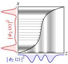
Figure 1: A sketch of a normalizing flow from a density $|\psi_{2}(x)|^{2}$ to a target density $|\phi_{2}(z)|^{2}$. Here, $\phi_{2}(z)$ is a wavefunction composed of second-order Hermite polynomials with two nodes. Notably, the flow can change the density distribution without changing the number of nodes.

The wavefunctions associated with the vibrational Hamiltonian are denoted by $|\Psi_{n}\rangle$, where the index $n$ distinct energy levels, and notably, $n=0$ identifies the ground state. These eigenstates constitute a set of orthogonal many-body states, with each state corresponding to an eigenvalue $E_{n}=\langle\Psi_{n}|H|\Psi_{n}\rangle$. To compute these wavefunctions using the variational method, choosing a good parameterization is crucial. A natural approach involves applying a unitary transformation to the non-interacting reference states $|\Psi_{n}\rangle=U|\Phi_{n}\rangle$, which are the wavefunctions for $D$-dimensional harmonic oscillators. This canonical transformation is realized via a parameterized and learnable bijection that maps the normal coordinates $\bm{x}$ to a set of new coordinates $\bm{z}$ in $D$-dimensional space, i.e., the normalizing flow Dinh et al. (2014); Germain et al. (2015); Rezende and Mohamed (2016); Dinh et al. (2016); Papamakarios (2019); Papamakarios et al. (2021); Saleh et al. (2023); Lei (2018), $f:\bm{x}\rightarrow\bm{z}$, and the associated parameters of this transformation are denoted as $\bm{\theta}$. The normalizing flow serves as an elaboration of the backflow transformation through the application of invertible neural networks, offering a modern approach to handling transformations. The many-body wavefunction is then articulated as follows Xie et al. (2022, 2023a, 2023b); Saleh et al. (2023):

$$\Psi_{n}(\bm{x})=\Phi_{n}(\bm{z})\left|\text{det}\left(\frac{\partial\bm{z}}{\partial\bm{x}}\right)\right|^{\frac{1}{2}},$$ (2)

where $\Psi_{n}(\bm{x})=\langle\bm{x}|\Psi_{n}\rangle$, and $\Phi_{n}(\bm{z})=\langle\bm{z}|\Phi_{n}\rangle$. Here, the variational wavefunction is dependent on parameters $\Psi_{n}(\bm{\theta},\bm{x})=U(\bm{\theta})\Phi_{n}(\bm{z})$, where the parameters $\bm{\theta}$ are typically omitted for brevity in Eq. (2). For more detailed information on the basis states, please refer to Appendix A. We also represent a normalizing flow from a complex distribution to a simple distribution in FIG. 1, which shows that the flow establishes a bijection between two distinct distributions without changing the topological structure Papamakarios et al. (2021), i.e. the number of nodes in the wavefunction.

The unitary transformation, generated by the square root of the Jacobian determinant $U(\bm{\theta})=\left|\text{det}\left({\partial\bm{z}}/{\partial\bm{x}}\right)\right|^{1/2}$, plays a critical role in introducing correlations among various vibrational modes, thereby effectively approximating complicated many-body wavefunctions. This transformation is also known as a point transformation, as delineated in Refs. DeWitt (1952); Eger and Gross (1963, 1964); Witriol (1972). The use of a set of orthogonal basis states $\Phi_{n}(\bm{z})$ alongside the square root of the Jacobian determinant is pivotal in our method. This mathematical structure ensures that the transformed wavefunctions $\Psi_{n}(\bm{x})$ maintain their orthogonality. This property is articulated through the following equation Xie et al. (2022, 2023a, 2023b); Saleh et al. (2023):

$$\int d\bm{x}\Psi^{*}_{n^{\prime}}(\bm{x})\Psi_{n}(\bm{x})=\delta_{nn^{\prime}}.$$ (3)

It is worth emphasizing that our variational wavefunction markedly diverges from those traditionally used in the VSCF method Bowman (1978, 1986); Gerber and Ratner (1979); Thompson and Truhlar (1982). Our formulation incorporates an additional Jacobian determinant, substantially amplifying the expressive capabilities of the wavefunction. This modification not only augments the theoretical framework but also enhances the potential for capturing intricate interactions in vibrational systems.

Crucially, our approach eliminates the reliance on the specific form of the PES, which can be represented in various forms, including series expansions, neural networks, or even density functional theory (DFT) programs. This flexibility contrasts sharply with methods like the RRBPM and LOBPCG Leclerc and Carrington (2014); Thomas and Carrington Jr (2015); Rakhuba and Oseledets (2016); Knyazev (2001), where the PES is required to be delineated as a sum of products. Such a specification introduces inherent inaccuracies to the PES, particularly when constructing the cubic and quartic terms of the force field, and complicates the incorporation of higher-order terms for enhanced precision. Hence, our approach provides a significant advantage by avoiding the extra errors common in the series expansion of the PES, ensuring a broader applicability and increased accuracy in modeling complex vibrational systems.

Next, we focus on optimizing the variational wavefunctions for all target states, including both the ground and excited states. The primary goal is to determine the optimal coefficients $\bm{\theta}$ for the normalizing flow $f$. Within this framework, the loss function can be succinctly defined as the summation of energies across all states:

$$\mathcal{L}=\sum_{n=1}^{M}\underset{\bm{x}\sim|\Psi_{n}(\bm{x})|^{2}}{\large{\mathbb{E}}}E_{n}^{\text{loc}}(\bm{x}),$$ (4)

where ${\large{\mathbb{E}}}$ represents the expectation over samples $\bm{x}$ drawn from the probability distribution $|\Psi_{n}(\bm{x})|^{2}$, and $M$ denotes the number of states targeted for computation. The local energies are associated with the variational wavefunctions:

$$E_{n}^{\text{loc}}(\bm{x})= -\sum_{i=1}^{D}\left[\frac{\partial^{2}}{\partial x_{i}^{2}}\ln|\Psi_{n}(\bm{x})|+\left(\frac{\partial}{\partial x_{i}}\ln|\Psi_{n}(\bm{x})|\right)^{2}\right]$$ (5)

$$+V(\bm{x}),$$

where the gradient and laplacian of the wavefunction, crucial for measuring the kinetic energy, can be computed efficiently through automatic differentiation. This technique, supported by popular computational packages such as JAX Bradbury et al. (2018) and PyTorch Paszke et al. (2019), offers significant advantages in terms of speed and accuracy over traditional numerical differentiation methods. Furthermore, our method exhibits linear computational complexity $\mathcal{O}(M)$ dependent on the number of state samplings, as demonstrated by Eq. (4).

In the training procedure, the optimization of parameters is essential through the gradient of the loss function, which can be derived from Eq. (4) and Eq. (5). It is also referred in the Refs. Xie et al. (2022, 2023a):

$$\nabla_{\bm{\theta}}\mathcal{L}=2\sum_{n=1}^{M}\underset{\bm{x}\sim|\Psi_{n}(\bm{x})|^{2}}{\large{\mathbb{E}}}\left[E_{n}^{\text{loc}}(\bm{x})~{}\nabla_{\bm{\theta}}\ln|\Psi_{n}(\bm{x})|\right].$$ (6)

In summary, the entire process of the neural canonical transformation approach for determining the energy levels of vibrational systems is outlined in Algorithm 1.

Algorithm 1 Energy levels in vibrational systems

0:   Potential energy surface $V(\bm{x})$

0:   Energy levels $E_{n}$

1:  Initialize $\Psi_{n}(\bm{\theta},\bm{x})=U(\bm{\theta})\Phi_{n}(\bm{z})$

2:  while $\mathcal{L}$ is not converged do

3:         MCMC Sampling $\bm{x}\sim|\Psi_{n}(\bm{\theta},\bm{x})|^{2}$

4:         Compute $\mathcal{L}$ and $\nabla_{\bm{\theta}}\mathcal{L}$.

5:         Optimize $\bm{\theta}$ with $\nabla_{\bm{\theta}}\mathcal{L}$.

6:  end while

7:  Measure $E_{n}=\mathbb{E}_{\bm{x}\sim|\Psi_{n}(\bm{x})|^{2}}E_{n}^{\text{loc}}(\bm{x})$.

III Applications

III.1 64-dimensional coupled oscillator

To evaluate the effectiveness of our method, we first computed a coupled harmonic oscillator system with $D=64$ dimensions, serving as a benchmark for testing. This system exclusively features quadratic interaction terms, making it exactly solvable, and a detailed analytical study is provided in Appendix B. The Hamiltonian of the $D$-dimensional coupled harmonic oscillator is specified as follows Rakhuba and Oseledets (2016); Leclerc and Carrington (2014); Thomas and Carrington Jr (2015):

$$H=\sum_{i=1}^{D}\frac{1}{2}\left(-\frac{\partial^{2}}{\partial x_{i}^{2}}+\omega_{i}^{2}x_{i}^{2}\right)+\sum_{i>j}^{D}\alpha_{ij}\sqrt{\omega_{i}\omega_{j}}x_{i}x_{j},$$ (7)

where we set the frequency for the $i$-th mode as $\omega_{i}=\sqrt{i/2}$, and the coupling constant is uniformly chosen as $\alpha_{ij}=0.1$ for all $i>j$, aligning with the parameters used in prior studies Rakhuba and Oseledets (2016); Leclerc and Carrington (2014); Thomas and Carrington Jr (2015) This coupling arrangement induces modifications in both the frequency and excited state energies, and the primary objective for us is to compute the lowest $M=80$ eigenstates and their corresponding eigenvalues.

In the following computation, we employed a neural network called RNVP Dinh et al. (2016) to parameterize the coordinate transformation $f:\bm{x}\rightarrow\bm{z}$, and a concise introduction to this network is presented in Appendix C. For this particular benchmark, the RNVP network is configured with $16$ coupling layers, where each coupling layer consists of a multilayer perceptron (MLP) with $2$ hidden layers and a width of $128$. Consequently, the total number of parameters reaches $661568$. In the following of this paper, the set of hyperparameters is denoted as $\{16,128,2\}$. A notable advantage of this network is its ability to construct a lower triangular Jacobian determinant, facilitating the efficient computation of the logarithm of the Jacobian determinant $\log|\partial\bm{z}/\partial\bm{x}|$.

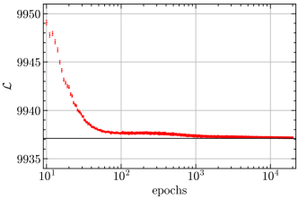
Figure 2: The optimization process of a $64$-dimensional coupled harmonic oscillator. The black line represents the values of the analytical solution $\sum_{n=1}^{80}E_{n,\text{exact}}$, while the red line depicts the loss function $\mathcal{L}$ with $M=80$ states.

The training batch size is set to $2048$, which indicates that $2048\times 80$ states are sampled through MCMC in each epoch. The initial parameters of the network are initialized in proximity to an identity transformation, which implies that the initial variational wavefunctions approximate the harmonic oscillator wavefunctions closely. The well-known adaptive moment estimation (ADAM) Kingma and Ba (2014) optimizer is employed for optimization. FIG. 2 illustrates the evolution of the loss function with respect to the number of iterations. After $20000$ epochs, the loss function converges to a value of $\mathcal{L}=9937.186(15)$ energy unit, which is in close approximation to the analytical solution $\sum_{n=1}^{m}E_{n,\text{exact}}=9937.108$.

Table 1: A subset of the $M=80$ lowest energy levels of a $64$-dimensional coupled oscillator. In this table, “$n$” denotes the level index, “Assignment” indicates the normal mode assignment, “$E_{\text{exact}}$” represents the exact solution, “$E_{\text{num}}$” corresponds to the numerical results obtained through neural network calculations, the fifth row provides information on the relative error, and ZPE is an abbreviation for “zero-point energy”, i.e. the ground state energy.

$n$	Assignment	$E_{n,\text{exact}}~{}$	$E_{n,\text{num}}~{}$	$\frac{E_{\text{num}}-E_{\text{exact}}}{E_{\text{exact}}}$
$0$	ZPE	$121.6209$	$121.6218$	$7.4\times 10^{-6}$
$1$	$\nu_{1}$	$122.2924$	$122.2931$	$6.1\times 10^{-6}$
$2$	$\nu_{2}$	$122.5856$	$122.5864$	$6.5\times 10^{-6}$
$3$	$\nu_{3}$	$122.8106$	$122.8115$	$7.7\times 10^{-6}$
$4$	$2\nu_{1}$	$122.9638$	$122.9646$	$6.5\times 10^{-6}$
$5$	$\nu_{4}$	$123.0002$	$123.0014$	$9.7\times 10^{-6}$
$6$	$\nu_{5}$	$123.1673$	$123.1682$	$7.5\times 10^{-6}$
$7$	$\nu_{1}+\nu_{2}$	$123.2570$	$123.2583$	$9.8\times 10^{-6}$
$8$	$\nu_{6}$	$123.3183$	$123.3197$	$1.1\times 10^{-5}$
$9$	$\nu_{7}$	$123.4572$	$123.4586$	$1.2\times 10^{-5}$
$19$	$2\nu_{1}+\nu_{2}$	$123.9285$	$123.9295$	$8.3\times 10^{-6}$
$29$	$\nu_{3}+\nu_{4}$	$124.1899$	$124.1910$	$9.5\times 10^{-6}$
$39$	$2\nu_{4}$	$124.3795$	$124.3809$	$1.2\times 10^{-5}$
$49$	$\nu_{2}+\nu_{8}$	$124.5512$	$124.5524$	$9.7\times 10^{-6}$
$59$	$\nu_{4}+\nu_{6}$	$124.6976$	$124.6993$	$1.4\times 10^{-5}$
$69$	$3\nu_{1}+\nu_{3}$	$124.8248$	$124.8258$	$7.5\times 10^{-6}$
$79$	$2\nu_{1}+\nu_{8}$	$124.9293$	$124.9303$	$8.1\times 10^{-6}$

Following this, we conducted a comprehensive measurement of all $M=80$ energy levels. Owing to limitations in space, only a subset of these values is displayed in TABLE 1. A comparison with exact solutions reveals that the relative error of our numerical results typically falls within the order of $10^{-6}$, while the absolute error spans from $0.001$ to $0.004$ energy units, demonstrating high precision in our calculations. In previous tensor-based methods, such RRBPM Leclerc and Carrington (2014) and LOBPCG Rakhuba and Oseledets (2016), have shown diminished accuracy for higher excited states, primarily due to the challenges posed by increased entanglement. As mentioned in Refs. Thomas and Carrington Jr (2015); Leclerc and Carrington (2014), the relative errors varying from $10^{-7}$ to $10^{-3}$. In contrast, the variational wavefunctions are independent of entanglement in our method, ensuring consistent accuracy across all states, while the equal weights of all states in the computation of the loss function.

It’s noteworthy that utilizing the same RNVP network size $\{16,128,2\}$ to exclusively optimize the ground state wavefunction, i.e., setting the number of states $M=1$, yields more accurate results. Under this condition, the ground state energy eventually converges to $E_{0,\text{num}}=121.620968(19)$ after $20000$ epochs. This represents a relative error of just $1.7\times 10^{-7}$ compared to the exact solution $E_{0,\text{exact}}=121.620948$, enhancing the precision by an order of magnitude compared to the “ZPE” in TABLE 1. This demonstrates the superior accuracy of our neural canonical transformation method over the H-RRBPM Thomas and Carrington Jr (2015).

In reality, the application of our method to a $64$-dimensional coupled oscillator may not fully demonstrate its unique advantages. Because the square root of the Jacobian determinant, in Eq. (2), plays a relatively simple role, which only serves to scale the coordinates (refer to Appendix B) without adding additional correlation effects to the system. Despite this, as a benchmark test, it provides evidence of the reliability of the neural canonical transformation method in solving the variational Hamiltonians.

III.2 Acetonitrile

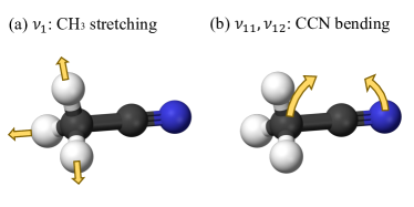
Figure 3: Two typical vibrational modes of acetonitrile ($\text{C}\text{H}_{3}\text{CN}$) with $C_{3v}$ symmetry. The black, white and blue spheres represent C, H and N atoms respectively. The vibrational mode $\nu_{1}$ has $\text{A}_{1}$ symmetry, while mode $\nu_{11}$ and $\nu_{12}$ have E symmetry.

Building on the discussion of the toy model in the preceding subsection, we turn our attention to real molecules, which exhibit multiple vibrational modes. This exploration is critically important for our study, as it allows comparison with other numerical methods and experimental findings. Specifically, we have undertaken computational analyses on the acetonitrile ($\text{C}\text{H}_{3}\text{CN}$), a molecule that has been extensively studied Herzberg (1960); Nakagawa and Shimanouchi (1962); Koivusaari et al. (1992); Tolonen et al. (1993); Andrews and Boxer (2000); Paso et al. (1994); Duncan et al. (1978); Nakagawa et al. (1985); Begue et al. (2005); Thomas and Carrington Jr (2015); Leclerc and Carrington (2014); Avila and Carrington (2011); Odunlami et al. (2017). It consists of 6 atoms and has $D=12$ vibrational modes, displaying $C_{3v}$ symmetry. Using the same symbols as presented in Ref. Thomas and Carrington Jr (2015), the vibrational modes $\nu_{1},~{}\nu_{2},~{}\nu_{3},~{}\nu_{4}$ are characterized by $\text{A}_{1}$ symmetry. Meanwhile, the modes $\nu_{5},~{}\nu_{7},~{}\nu_{9},~{}\nu_{11}$ along with their degenerate counterparts $\nu_{6},~{}\nu_{8},~{}\nu_{10},~{}\nu_{12}$ are described by E symmetry. As illustrative instances, FIG. 3 displays two characteristic vibrational modes, as elaborated in Ref. Begue et al. (2005).

In the following computing, we used the same PES as described in the Refs. Thomas and Carrington Jr (2015); Avila and Carrington (2011); Begue et al. (2005), which contains $12$ quadratic, $108$ cubic, and $191$ quartic terms, and it is publicly accessible in our code myc . Despite the increased complexity of this PES, our method navigates the intricacies of such a vibrational Hamiltonian with proficiency. It is important to clarify that our approach does not necessitate a polynomial expansion of the PES. The decision to utilize the same force field was driven by our aim to enable direct, meaningful comparisons with the findings reported in Refs. Leclerc and Carrington (2014); Thomas and Carrington Jr (2015); Avila and Carrington (2011).

Table 2: Comparison of Acetonitrile’s Zero-Point Energies (ZPE) (in $\text{cm}^{-1}$) across various numerical methods. Our method is uniquely focused on the ground state ($M=1$) only.

Method	ZPE
RRBPMLeclerc and Carrington (2014)	$9837.6293$
H-RRBPM Thomas and Carrington Jr (2015)	$9837.429$
Smolyak Thomas and Carrington Jr (2015); Avila and Carrington (2011)	$9837.4073$
RNVP {16, 128, 2}	$9837.40(2)$
RNVP {16, 256, 2}	$9837.42(3)$
RNVP {32, 128, 2}	$9837.39(3)$
RNVP {64, 64, 2}	$9387.39(2)$

At the beginning of this example, our attention was dedicated to the optimization of the ground state wavefunction utilizing RNVP networks of various sizes. We specified the number of states as $M=1$, explicitly indicating our objective to exclusively explore the ground state. The numerical results in the energy unit of wavenumbers ($\text{cm}^{-1}$) are presented in the TABLE 2, and juxtaposed with findings from alternative numerical approaches Leclerc and Carrington (2014); Thomas and Carrington Jr (2015). For the purpose of our sampling was confined to the ground state, we chose a sufficiently large training batch size of $65536$. After training, we increased the batch size to $524288$ for energy measurement to eliminate the error bar.

The comparison of energy values derived from all considered methods reveals a remarkable consistency, with discrepancies confined to the first decimal place and not exceeding $0.2~{}\text{cm}^{-1}$. Our method yields a ground state energy $E_{0}=9387.39(2)~{}\text{cm}^{-1}$ with the RNVP network $\{64,64,2\}$, which is marginally lower than the energies obtained via the RRBPM and H-RRBPM, yet aligns closely with the outcomes produced by Smolyak’s approach. Notably, the precision of our energy estimations, reliant on Monte Carlo sampling, is inherently bound by the selected batch size. As a result, enhancing accuracy and diminishing the margin of error present substantial challenges.

Table 3: Experimental and numerical energies (in $\text{cm}^{-1}$) of acetonitrile. The lowest $M=84$ states have been trained in the normalizing flow. The excited state energies are adjusted relative to the ground state energy $E_{n}-E_{0}$. The Smolyak Quadrature Calculation results are labeled as $E_{\text{Smo}}$. In the row of RNVP, “U” indicates uniform weighting across all states, while “H” signifies that the ground state’s weight constitutes half of the total for all states.

$n$	Assignment	Experiment	Pert-Var	H-RRBPM	Smolyak	RNVP(U){16,128,2}		RNVP(H){16,128,2}
		Nakagawa and Shimanouchi (1962); Duncan et al. (1978); Nakagawa et al. (1985); Koivusaari et al. (1992); Tolonen et al. (1993); Paso et al. (1994); Andrews and Boxer (2000)	Begue et al. (2005)	Thomas and Carrington Jr (2015)	Thomas and Carrington Jr (2015); Avila and Carrington (2011)	$E$	$E-E_{\text{Smo}}$	$E$	$E-E_{\text{Smo}}$
$0$	ZPE	$-$	$-$	$9837.429$	$9837.407$	$9838.73$	$1.33$	$9838.02$	$0.62$
$1$	$\nu_{11}$	$362,365$	$366.0$	$361.00$	$360.991$	$360.71$	$-0.28$	$360.97$	$-0.02$
$3$	$2\nu_{11}$	$717$	$725.0$	$723.22$	$723.181$	$723.44$	$0.25$	$723.66$	$0.48$
$4$	$\nu_{11}+\nu_{12}$	$739$	$731.0$	$723.87$	$723.827$	$722.85$	$-0.98$	$723.17$	$-0.65$
$6$	$\nu_{4}$	$916,920$	$916.0$	$900.71$	$900.662$	$898.83$	$-1.83$	$903.49$	$2.83$
$7$	$\nu_{9}$	$1041,1042$	$1038.0$	$1034.19$	$1034.126$	$1034.56$	$0.44$	$1034.81$	$0.68$
$9$	$3\nu_{11}$	$1122$	$1098.0$	$1086.66$	$1086.554$	$1087.94$	$1.39$	$1088.16$	$1.60$
$12$	$3\nu_{12}$	$1122$	$1098.0$	$1086.66$	$1086.554$	$1087.81$	$1.26$	$1088.30$	$1.74$
$10$	$2\nu_{11}+\nu_{12}$	$1077$	$1094.0$	$1087.88$	$1087.776$	$1086.66$	$-1.11$	$1087.38$	$-0.40$
$13$	$\nu_{4}+\nu_{11}$	$1290$	$1282.0$	$1259.90$	$1259.822$	$1257.97$	$-1.85$	$1261.91$	$2.08$
$15$	$\nu_{3}$	$1390,1385$	$1400.0$	$1389.16$	$1388.973$	$1396.64$	$7.67$	$1396.06$	$7.09$
$16$	$\nu_{9}+\nu_{11}$	$1410,1409$	$1401.0$	$1394.79$	$1394.689$	$1394.59$	$-0.10$	$1395.44$	$0.75$
$17$	$\nu_{10}+\nu_{11}$	$1402$	$1398.0$	$1395.01$	$1394.907$	$1395.04$	$0.13$	$1395.81$	$0.90$
$18$	$\nu_{9}+\nu_{12}$	$1402$	$1398.0$	$1397.85$	$1397.687$	$1395.25$	$-2.44$	$1395.73$	$-1.96$
$21$	$3\nu_{11}+\nu_{12}$	$1448$	$1467.0$	$1453.08$	$1452.827$	$1452.34$	$-0.48$	$1452.84$	$0.01$
$25$	$\nu_{7}$	$1453,1450$	$1478.0$	$1483.30$	$1483.229$	$1485.60$	$2.37$	$1485.48$	$2.25$
$27$	$\nu_{4}+2\nu_{11}$	$-$	$1647.0$	$1620.45$	$1620.222$	$1618.58$	$-1.64$	$1622.05$	$1.83$
$28$	$\nu_{4}+\nu_{11}+\nu_{12}$	$-$	$1645.7$	$1620.99$	$1620.767$	$1618.03$	$-2.73$	$1621.57$	$0.80$
$30$	$\nu_{3}+\nu_{11}$	$-$	$1766.4$	$1749.76$	$1749.530$	$1757.57$	$8.04$	$1757.24$	$7.71$
$32$	$\nu_{9}+2\nu_{11}$	$-$	$1761.6$	$1756.60$	$1756.426$	$1756.83$	$0.40$	$1757.40$	$0.97$
$37$	$\nu_{10}+2\nu_{12}$	$-$	$1761.6$	$1756.60$	$1756.426$	$1756.44$	$0.02$	$1757.45$	$1.02$
$34$	$\nu_{9}+\nu_{11}+\nu_{12}$	$-$	$1767.4$	$1757.30$	$1757.133$	$1756.73$	$-0.40$	$1757.35$	$0.21$
$33$	$\nu_{10}+2\nu_{11}$	$-$	$1769.3$	$1759.98$	$1759.772$	$1757.50$	$-2.27$	$1758.10$	$-1.67$
$44$	$2\nu_{4}$	$-$	$1833.7$	$1785.37$	$1785.207$	$1792.26$	$7.05$	$1802.34$	$17.13$
$46$	$\nu_{8}+\nu_{11}$	$-$	$1838.2$	$1844.36$	$1844.258$	$1845.96$	$1.70$	$1846.04$	$1.78$
$47$	$\nu_{7}+\nu_{12}$	$-$	$1838.2$	$1844.79$	$1844.690$	$1846.48$	$1.79$	$1846.64$	$1.95$
$45$	$\nu_{7}+\nu_{11}$	$-$	$1842.2$	$1844.43$	$1844.330$	$1846.58$	$2.25$	$1846.80$	$2.47$
$49$	$\nu_{4}+\nu_{9}$	$-$	$1952.3$	$1931.70$	$1931.547$	$1932.51$	$0.97$	$1937.27$	$5.73$
$51$	$\nu_{4}+3\nu_{11}$	$-$	$2010.3$	$1982.14$	$1981.849$	$1981.05$	$-0.80$	$1983.75$	$1.90$
$54$	$\nu_{4}+3\nu_{12}$	$-$	$2010.3$	$1982.14$	$1981.849$	$1981.41$	$-0.44$	$1984.24$	$2.39$
$52$	$\nu_{4}+2\nu_{11}+\nu_{12}$	$-$	$2015.1$	$1983.14$	$1982.857$	$1980.05$	$-2.81$	$1982.93$	$0.07$
$56$	$\nu_{9}+\nu_{10}$	$2075$	$2059.0$	$2057.17$	$2057.068$	$2065.40$	$8.33$	$2066.40$	$9.33$
$55$	$2\nu_{9}$	$2082$	$2067.0$	$2065.38$	$2065.286$	$2063.61$	$-1.68$	$2065.12$	$-0.16$
$58$	$\nu_{3}+2\nu_{11}$	$-$	$2131.3$	$2111.75$	$2111.380$	$2120.29$	$8.91$	$2120.23$	$8.85$
$59$	$\nu_{3}+\nu_{11}+\nu_{12}$	$-$	$2130.0$	$2112.67$	$2112.297$	$2119.34$	$7.05$	$2119.56$	$7.27$
$61$	$\nu_{9}+3\nu_{11}$	$-$	$2135.4$	$2119.66$	$2119.327$	$2120.56$	$1.23$	$2121.20$	$1.88$
$63$	$\nu_{9}+2\nu_{11}+\nu_{12}$	$-$	$2134.5$	$2120.84$	$2120.541$	$2119.89$	$-0.65$	$2120.54$	$-0.00$
$64$	$\nu_{10}+2\nu_{11}+\nu_{12}$	$-$	$2130.5$	$2121.21$	$2120.910$	$2120.02$	$-0.89$	$2120.86$	$-0.05$
$62$	$\nu_{10}+3\nu_{11}$	$-$	$2130.2$	$2123.16$	$2122.834$	$2121.66$	$-1.18$	$2122.30$	$-0.53$
$65$	$\nu_{9}+\nu_{11}+2\nu_{12}$	$-$	$2130.5$	$2123.63$	$2123.301$	$2120.14$	$-3.16$	$2121.17$	$-2.13$
$76$	$2\nu_{4}+\nu_{11}$	$-$	$2199.4$	$2142.68$	$2142.614$	$2149.64$	$7.02$	$2158.37$	$15.76$
$78$	$\nu_{7}+2\nu_{11}$	$2192$	$2203.0$	$2206.79$	$2206.626$	$2209.37$	$2.74$	$2210.00$	$3.38$
$83$	$\nu_{8}+2\nu_{12}$	$2192$	$2203.0$	$2206.80$	$2206.633$	$2208.96$	$2.32$	$2209.46$	$2.82$
$79$	$\nu_{8}+2\nu_{11}$	$-$	$2210.4$	$2206.95$	$2206.776$	$2208.56$	$1.79$	$2208.94$	$2.16$
$80$	$\nu_{7}+\nu_{11}+\nu_{12}$	$-$	$2208.3$	$2207.72$	$2207.559$	$2208.49$	$0.93$	$2209.31$	$1.75$

Furthermore, our study extended to calculating the lowest $M=84$ excited states, using RNVP networks of various sizes. The corresponding numerical results along with the relevant experimental data Nakagawa and Shimanouchi (1962); Duncan et al. (1978); Nakagawa et al. (1985); Koivusaari et al. (1992); Tolonen et al. (1993); Paso et al. (1994); Andrews and Boxer (2000) and numerical values Begue et al. (2005); Thomas and Carrington Jr (2015) are detailed in TABLE 3. It’s noteworthy that the results for certain degenerate excited states are not listed due to their near-identical energy values, which fall within the confines of the E symmetry group. By way of illustration, the energies for the excited states with assignment $\nu_{11}$ and $\nu_{12}$ are found to be $E_{\nu_{11}}=10199.52(8)~{}\text{cm}^{-1}$ and $E_{\nu_{12}}=10199.49(8)~{}\text{cm}^{-1}$, respectively, showcasing a negligible difference within the statistical error bar.

With the objective of training a substantial number of states, we configured the batch size to $1024$, resulting in the sampling of $1024\times 84$ states per epoch. In the loss function Eq. (4), the weights of these states are uniform, denoted as “RNVP(U)” in the table. To improve the neural network’s ability to accurately represent the ground state, we explored the strategy of disproportionately increasing the ground state’s sampling frequency within the loss function. Specifically, we adjusted the sampling frequency so that the ground state accounts for half of all sampled states, which we denote as “RNVP(H)”. It is also aligned with the variational principle Gross et al. (1988). Despite this modification, the batch size remains $1024$, meaning that the ground state being sampled $1024\times 83$ times in each epoch, while the remaining $83$ excited states each receive $1024$ samples.

Comparing the ground state energies listed in TABLEs 3 and 2, it is observable that optimizing a large number of eigenstates simultaneously slightly elevates our ground state energy by approximately $1~{}\text{cm}^{-1}$. A comparison of the ZPE between RNVP(U) and RNVP(H) in Table 3 demonstrates that a greater weighting on the ground state during sampling results in a lower energy. This outcome arises because the neural network is required to cover coordinate transformations for both the ground and all excited states, thereby imposing a greater demand on the network’s expressive capacity.

The energies of nearly all our excited states are lower than those reported in Ref. Begue et al. (2005), where the perturbation variational method was employed, underscoring the efficacy of our neural canonical transformation approach. In comparison with results derived from tensor-based methods, such as Smolyak and H-RRBPM Thomas and Carrington Jr (2015); Avila and Carrington (2011), we have noticed some variations. Although some energy levels are slightly higher and others lower, the differences generally fall within a narrow band of several wavenumbers. Notably, certain individual energy levels, like $\nu_{9}+\nu_{10}$, exhibit more significant deviations but remain closer to experimental values.

Further analysis focusing on the layers of the RNVP network, including $\{16,128,2\}$ and $\{32,128,2\}$, indicated no significant differences, leading us to exclude these results from the table. We posit that the differences observed between our results and experiments can largely be ascribed to the inherent limitations of the PES accuracy, considering that the same PES was employed by the other numerical methods.

III.3 Ethylene oxide

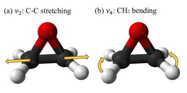
Figure 4: Two typical vibrational modes of ethylene oxide ($\text{C}_{2}\text{H}_{4}\text{O}$). The black, white and red spheres represent C, H and O atoms respectively.

It is both motivating and rewarding for us to advance our computational investigations to a more complex molecule, specifically ethylene oxide ($\text{C}_{2}\text{H}_{4}\text{O}$), which comprises $7$ atoms and possesses $15$ degrees of freedom. As depicted in FIG. 4, two typical vibrational modes are presented. Unlike acetonitrile, ethylene oxide is distinguished by its lack of degenerate vibrational modes and exhibits a lower symmetry. This molecule has been extensively studied through both experimental and computational techniques, as evidenced by a wealth of literature Lowe et al. (1986); Komornicki et al. (1983); Rebsdat and Mayer (2000); Begue et al. (2006); Cant and Armstead (1975); Lord and Nolin (1956); Schriver et al. (2004); Nakanaga (1980); Yoshimizu et al. (1975); Carbonnière et al. (2010); Thomas and Carrington Jr (2015). The same PES is taken in our calculation as described in Refs. Thomas and Carrington Jr (2015); Bégué et al. (2007), which comprises $15$ quadratic, $180$ cubic, and $445$ quartic terms myc .

Table 4: Zero-point energies (ZPE) (in $\text{cm}^{-1}$) of ethylene oxide from different numerical methods. The variational wavefunctions of the ground state ($M=1$) are optimized for various RNVP sizes.

Method	ZPE
VCI Bégué et al. (2007)	$12501$
VMFCI Bégué et al. (2007)	$12463.7$
VCI-P Carbonnière et al. (2010)	$12464.26$
H-RRBPM Thomas and Carrington Jr (2015)	$12461.86$
RNVP {16, 128, 2}	$12461.59(4)$
RNVP {16, 256, 2}	$12461.63(5)$
RNVP {32, 128, 2}	$12461.58(4)$
RNVP {64, 64, 2}	$12461.56(4)$

Similarly, we first train the neural network through the loss function Eq. (4) with $M=1$, employing a batch size of $65536$. The results, detailed in TABLE 4, are compared with outcomes from other numerical methods as referenced in Refs. Bégué et al. (2007); Carbonnière et al. (2010); Thomas and Carrington Jr (2015). The RNVP network with a size of $\{64,64,2\}$ achieves the lowest ground-state energy $E_{0}=12461.56~{}\text{cm}^{-1}$, surpassing the precision of other documented methods within the statistical error. Subsequent investigations into the effect of RNVP network sizes, particularly those with $16$, $32$, and $64$ coupling layers, demonstrated a clear positive relationship between increased depth and lower ground-state energy. However, enlarging the network’s width showed a marginal decline in performance. This phenomenon is linked to the network’s parameter count, which exceeds 1.2 million in $\{16,256,2\}$, complicating convergence and requiring longer to converge.

Table 5: Experimental and numerical energies (in wavenumber $\text{cm}^{-1}$) of ethylene oxide. The number of states that have been trained in the loss function is $M=170$. The excited state energies are corrected for the ground state background $E_{n}-E_{0}$. Data for gas, liquid, and solid phases represent experimental values. ${}^{\text{a}}$ The order of $n$ is taken from decoupled harmonic system. ${}^{\text{b}}$ $\nu_{6}$ and $\nu_{8}$ are respectively sourced from Ref. Cant and Armstead (1975) and Ref. Yoshimizu et al. (1975), while all others are obtained from Ref. Nakanaga (1980). ${}^{\text{c}}$ $\nu_{7}$ is an inactive infrared band type Lord and Nolin (1956). ${}^{\text{d}}$ $\nu_{2}$ for the amorphous phase, while others for the crystalline phase.

$n^{\text{a}}$	Assignment	Gas${}^{\text{b}}$	Liquid${}^{\text{c}}$	Solid${}^{\text{d}}$	VMFCI	VCI-P	H-RRBPM	RNVP(U)	RNVP(H)
		Nakanaga (1980); Cant and Armstead (1975); Yoshimizu et al. (1975)	Lord and Nolin (1956)	Schriver et al. (2004)	Bégué et al. (2007)	Carbonnière et al. (2010)	Thomas and Carrington Jr (2015)	{16,128,2}	{16,128,2}
$0$	ZPE	$-$	$-$	$-$	$-$	$12464.26$	$12461.86$	$12472.00$	$12462.97$
$138$	$\nu_{1}$	$3018$	$3005$	$3005.1$	$2919$	$2921$	$2920.93$	$3006.50$	$3019.39$
$11$	$\nu_{2}$	$1498$	$1490$	$-$	$1497$	$1502$	$1496.23$	$1505.52$	$1513.06$
$9$	$\nu_{3}$	$1270$	$1266$	$1265.8$	$1272$	$1275$	$1271.12$	$1270.05$	$1287.24$
$6$	$\nu_{4}$	$1148$	$1120$	$1147.2$	$1123$	$1127$	$1122.11$	$1122.20$	$1129.94$
$3$	$\nu_{5}$	$877$	$877$	$853.8$	$879$	$884$	$878.40$	$875.44$	$882.74$
$163$	$\nu_{6}$	$3065$	$3063$	$3073.3$	$3032$	$3032$	$3029.99$	$3066.26$	$3077.80$
$8$	$\nu_{7}$	$-$	$1345$	$1045.8$	$1149$	$1154$	$1148.64$	$1145.09$	$1150.43$
$4$	$\nu_{8}$	$1020$	$807$	$817.7$	$1019$	$1024$	$1017.68$	$1014.32$	$1019.82$
$136$	$\nu_{9}$	$3006$	$3019$	$2994.9$	$2913$	$2929$	$2912.48$	$3001.21$	$3015.61$
$10$	$\nu_{10}$	$1472$	$1470$	$1466.7$	$1468$	$1473$	$1467.93$	$1469.46$	$1473.00$
$5$	$\nu_{11}$	$1151$	$1153$	$1168.9$	$1125$	$1131$	$1124.65$	$1122.58$	$1128.00$
$2$	$\nu_{12}$	$840$	$892$	$858.8$	$823$	$827$	$822.10$	$818.34$	$825.88$
$168$	$\nu_{13}$	$3065$	$3079$	$3061.5$	$3041$	$3043$	$3041.79$	$3080.13$	$3092.60$
$7$	$\nu_{14}$	$1142$	$1143$	$1160.2$	$1147$	$1152$	$1146.44$	$1142.31$	$1149.21$
$1$	$\nu_{15}$	$821$	$821$	$796.3$	$794$	$800$	$793.29$	$788.01$	$794.23$
$70$	$2\nu_{3}$	$-$	$-$	$-$	$-$	$2545$	$2537.64$	$2545.34$	$2576.39$
$129$	$\nu_{4}+\nu_{8}+\nu_{12}$	$-$	$-$	$-$	$-$	$3032$	$2940.11$	$2953.46$	$2970.33$
$126$	$\nu_{7}+\nu_{8}+\nu_{15}$	$-$	$-$	$-$	$-$	$3053$	$2951.19$	$2945.65$	$2956.26$
$128$	$\nu_{8}+\nu_{11}+\nu_{12}$	$-$	$-$	$-$	$-$	$3056$	$2953.39$	$2951.20$	$2963.39$
$123$	$2\nu_{10}$	$-$	$2916$	$2904.2$	$-$	$2963$	$2960.45$	$2938.59$	$2945.27$
$130$	$\nu_{2}+\nu_{10}$	$-$	$-$	$2950.3$	$-$	$3032$	$2998.85$	$2976.43$	$2986.36$
$133$	$2\nu_{2}$	$-$	$2961$	$2914.9$	$-$	$3011$	$3005.90$	$3012.22$	$3026.20$

In addition, we extended our computation to the lowest $M=170$ states across various RNVP network sizes, presenting a significantly more complex challenge than our previous molecular studies. The experimental and computational data about these states are comprehensively detailed in TABLE 5, with data sourced from Refs. Cant and Armstead (1975); Lord and Nolin (1956); Schriver et al. (2004); Nakanaga (1980); Yoshimizu et al. (1975); Carbonnière et al. (2010); Thomas and Carrington Jr (2015). Upon comparison with the data in TABLE 4, it becomes evident that optimizing for multiple states concurrently may slightly diminish the precision of ground state energy estimations, introducing a deviation of approximately $10~{}\text{cm}^{-1}$. Moreover, a comparative evaluation of the ”RNVP(U)” and ”RNVP(H)” reveals a pronounced improvement in the accuracy of ground state energies when more weight is applied in training.

Table 5 presents our findings for the higher excited states, including $\nu_{1}$, $\nu_{6}$, $\nu_{9}$, and $\nu_{13}$, which aligns more closely with experimental data. When assigning a greater weight to sample the ground state in training, there is a larger error in the energy of the excited states, leading to most values in “RNVP(H)” being generally higher than those in “RNVP(U)”. This observation leads us to believe that adopting more advanced neural network models in place of the RNVP could markedly enhance the accuracy of these results.

IV Discussions

Let’s begin by comparing our approach with other related methods.

• It is important to emphasize that our neural canonical transformation approach fully integrates the vibrational self-consistent field (VSCF) method, which has been extensively studied in the literature Bowman (1978, 1986); Gerber and Ratner (1979); Thompson and Truhlar (1982). The VSCF method only consists of a direct product of the eigenstates of harmonic oscillators, which can be seen as a particular case within our variational wavefunction, where the Jacobian determinant in Eq. (2) is equal to one.

• In Ref. Ishii et al. (2022), the authors use a backflow transformation into coordinate to solve the vibrational Hamiltonian, without an additional Jacobian determinant in the variational wavefunctions. They do not guarantee the orthogonality between different states, and the direct measurement of energies undertaken in their approach breaks the variational principle, making the results unreliable.

• A recent study in Ref. Saleh et al. (2023) describes a normalizing flow parameterized by a residual neural network, and then combines the wavefunctions through superposition. However, due to the nonorthogonal wavefunctions, their methodology requires a considerable amount of time for numerically integrating energy across multiple dimensions, which stands in contrast to the efficiency of our approach that uses Monte Carlo sampling for energy measurement.

• When compared to another Ref. Pfau et al. (2024), our method views atoms as a vibrational system and uses orthogonal wavefunctions, rather than constructing a nonorthogonal basis. This perspective enables us to avoid the complexities of electronic wavefunctions and diagonalizations associated with the number of states, significantly reducing computational complexity. Whereas their method scales as $\mathcal{O}(M^{4})$ for $M$ states, our method achieves linear scaling, $\mathcal{O}(M)$.

• Our approach draws parallels with the “Hermite+flow” methodology outlined in Ref. Cranmer et al. (2019), which employs a combination of Hermite polynomials and normalizing flow to represent the variational wavefunctions. However, their analysis is restricted to single-particle transformations and does not extend to multi-particle systems. In contrast, our research is adaptable to molecules with multiple atoms.

As a result, our approach can be extended to molecules with many degrees of freedom, making it a more scalable and versatile option.

Several aspects of our numerical calculations warrant further discussion, The excited state wavefunctions of quantum harmonic oscillator have nodes, which means we need a larger number of MCMC steps for effective sampling. The reason behind this is that a large number of steps is essential to eliminate the correlation between consecutive samples, which is crucial for accurate simulations. This requirement diverges from the systems existing in two or three dimensions without nodes, as referred in Refs. Xie et al. (2023a, b). During the training process, we implemented 200 MCMC steps to guarantee convergence. After the networks were fully trained, we increased this number to 500 steps to measure the local energy of each target state.

In the analysis of an actual molecule, it is reasonable to consider our variational wavefunction as a small perturbation in comparison to the quantum harmonic oscillator. This approach is supported by the observation that non-harmonic contributions are generally much smaller than their harmonic counterparts in the PES. As a result, the system tends to converge more easily when compared to the interacting fermionic systems in Refs. Xie et al. (2023a, b), which eliminates the need for more computationally intensive optimization methods. Specifically, using the ADAM optimizer Kingma and Ba (2014) is sufficient, and there is no need for the stochastic reconfiguration (SR) optimizer Xie et al. (2023a); Becca and Sorella (2017) optimizer, which requires significant computational resources in both time and memory.

In Section II, for the sake of simplicity, we adopt an equal-weighted superposition approach within the loss function Eq. (4). Let us denote the weight associated with the $n$-th state during sampling as $w_{n}$, they must satisfy $w_{0}\geq w_{1}\geq w_{2}\ldots\geq w_{M}$ and $w_{i}>0$ in accordance with the variational principle Gross et al. (1988). This arrangement offers flexibility in adjusting weights, which is crucial when dealing with a neural network with limited expressive capabilities. For instance, increasing the weight of the ground state can improve the accuracy of the ground state energy, as evidenced in our studies on ethylene oxide and acetonitrile. Furthermore, it is practical to study the system via a density matrix, $\rho=\sum_{n}\mu_{n}|\Psi_{n}(\bm{x})\rangle\langle\Psi_{n}(\bm{x})|$, as mentioned in Refs.  Xie et al. (2022, 2023a); Cranmer et al. (2019), and introduce an extra hyperparameter, temperature, to adjust the probabilities of various states $\mu_{n}$.

Our method presents significant opportunities for improvement, particularly in fully leveraging the capabilities of normalizing flows. In theory, it can create a bijection between any probability distributions without changing the topological structure Papamakarios et al. (2021), i.e. the nodes of the wavefunction in our research. However, the numerical results indicate that the RNVP network has difficulty effectively covering coordinate transformations across a wide range of states as the number of optimized states $M$ increases. To overcome this challenge, we need a more powerful neural network that can significantly enhance the model’s expressive ability. For an enhanced neural network, several crucial attributes are necessary:

• The ability to perform beyond the linear transformations of RNVP’s coupling layers, enabling non-linear transformations.

• A specialized Jacobian determinant structure, such as lower triangular or block-diagonal, facilitates faster computation.

• It is essential for the network to support second-order differentiation to avoid instability in kinetic energy computations.

• Practical applications do not require the computation of inverse transformations, even though the neural canonical transformation theoretically needs to be bijective.

Given these considerations, several neural network models, such as the neural spline flow modelDurkan et al. (2019) and autoregressive model Wu et al. (2019); Liu et al. (2021); Xie et al. (2023a), have emerged as promising candidates for further exploration. It will be one of the key focuses of our future studies.

We have made our source codes and original data publicly available to encourage further development in this field myc . Our method is notably scalable, and requires no specific form of the PES. This flexibility allows for integrating advanced computational approaches of the potential energies, such as density functional theory Kohn and Sham (1965); Hohenberg and Kohn (1964) and machine learning force field. These enhancements aim to improve potential energies beyond simple polynomials, a key area of our future research endeavors. Moreover, leveraging machine learning strategies such as distributed training Goyal et al. (2017), enables our method to handle systems comprising hundreds of atoms efficiently. This capability is especially beneficial for studying complex molecular, including proteins. We also plan to extend our approach to investigate the vibrational properties of solid systems, focusing on phonons Monserrat et al. (2013); Monacelli et al. (2021), as another main area of future research. Given these prospects, we are highly optimistic about the future evolution of neural canonical transformations in solving vibrational Hamiltonians.

Appendix A Basis state of variational wavefunction

In the variational wavefunctions, as presented by Eq. (2), we adopt the wavefunctions of a non-interacting harmonic oscillator in $D$ dimensions as the basis states. The corresponding Hamiltonian is given by:

$$H=\sum_{i=1}^{D}\frac{1}{2}\left(-\frac{\partial^{2}}{\partial z_{i}^{2}}+\omega_{i}^{2}z_{i}^{2}\right).$$ (8)

The eigenstate can be expressed as the direct product of a series of wavefunctions:

$$\Phi_{n}(\bm{z})=\phi_{n_{1}}(z_{1})~{}\phi_{n_{2}}(z_{2})~{}...~{}\phi_{n_{D}}(z_{D}),$$ (9)

where $\phi_{n_{i}}(z_{i})$ represents the eigenstates of a one-dimensional harmonic oscillator with frequency $\omega_{i}$:

$$\phi_{n_{i}}(z_{i})=\exp\left(-\frac{1}{2}\omega_{i}z_{i}^{2}\right)H_{n_{i}}\left(-\sqrt{{\omega_{i}}}z_{i}\right).$$ (10)

In the above wavefunction, we have ignored the normalization factor, $n_{i}$ is the energy level of the $i$-th oscillator, and $H_{n_{i}}$ is the $n_{i}$-th order Hermite polynomial. Then, the variational wavefunction is:

$$\Psi_{n}(x_{1},x_{2},...,x_{D}) =\phi_{n_{1}}(z_{1})~{}\phi_{n_{2}}(z_{2})~{}...~{}\phi_{n_{D}}(z_{D})$$ (11)

$$~{}~{}~{}~{}~{}~{}\times\sqrt{\left|\text{det}\frac{\partial(z_{1},z_{2},...,z_{D})}{\partial(x_{1},x_{2},...,x_{D})}\right|}.$$

Appendix B Exact solution of D-dimensional coupled oscillator

As mentioned in the main text of the article Eq. (7), the potential term of $D$-dimensional coupled harmonic oscillators is given by Rakhuba and Oseledets (2016); Leclerc and Carrington (2014); Thomas and Carrington Jr (2015):

$$V=\sum_{i=1}^{D}\frac{1}{2}\omega_{i}^{2}x_{i}^{2}+\sum_{i>j}^{D}\alpha_{ij}\sqrt{\omega_{i}\omega_{j}}x_{i}x_{j},$$ (12)

where the coupling constant is taken as $\alpha_{ij}=\alpha~{}(i>j)$. Also, the potential can be expressed in matrix form:

$$V=\frac{1}{2}\bm{x}^{T}\bm{A}\bm{x},$$ (13)

where $\bm{x}=(x_{1},x_{2},...,x_{D})^{T}$, and $\bm{A}$ is a $D\times D$ positive-definite real-symmetric matrix with diagonal elements $\bm{A}_{ii}=\omega_{i}^{2}$ and off-diagonal elements $\bm{A}_{ij}=\alpha\sqrt{\omega_{i}\omega_{j}}$. It could be exactly diagonalized as:

$$\bm{A}=\bm{P}\bm{\mathnormal{\Lambda}}\bm{P}^{T},$$ (14)

where $\bm{P}$ is a unitary matrix consisting of a series of eigenvectors, which satisfied $\bm{P}^{T}\bm{P}=\bm{P}\bm{P}^{T}=\bm{I}$, and $\bm{\mathnormal{\Lambda}}=\text{diag}(\nu_{1}^{2},\nu_{2}^{2},...,\nu_{D}^{2})$ is a diagonal matrix composed of eigenvalues. Taking the square root of these eigenvalues yields a set of new frequencies $\nu_{i}$. The exact solutions for the energy levels of $D$-dimensional coupled oscillators can be obtained by combining these frequencies:

$$E_{n_{1},n_{2},...n_{D}}=\sum_{i=1}^{D}\left(n_{i}+\frac{1}{2}\right)\nu_{i}.$$ (15)

In Eq. (9), it is noted that the harmonic oscillator’s frequency in the new coordinate $\bm{z}$ is $\omega_{i}$. An additional step is required to incorporate a scaling operation to transform the frequency from $\nu_{i}$ to $\omega_{i}$. Thus, the relationship between the new coordinates and the original coordinates involves a unitary transformation $\bm{P}^{T}$ and a scaling operation $\bm{\mathnormal{\Gamma}}$, i.e.:

$$\bm{z}=\bm{\mathnormal{\Gamma}}\bm{P}^{T}\bm{x},$$ (16)

where $\bm{\mathnormal{\Gamma}}=\text{diag}(\sqrt{\nu_{1}/\omega_{1}},\sqrt{\nu_{2}/\omega_{2}},...,\sqrt{\nu_{D}/\omega_{D}})$. It is known that the Jacobian of unitary transformation $\bm{P}^{T}$ is a unit matrix, hence the Jacobian determinant is only associated with the scaling operation:

$$\left|\text{det}\left(\frac{\partial\bm{z}}{\partial\bm{x}}\right)\right|=\prod_{i=1}^{D}\sqrt{\frac{\nu_{i}}{\omega_{i}}}.$$ (17)

Appendix C Normalizing flow for variational wavefunction

It is essential to clarify that our goal is to parameterize the normalizing flow from the normal coordinates $\bm{x}$ to a set of new coordinates $\bm{z}$. The well-known real-valued non-volume preserving (RNVP) Dinh et al. (2016) is used to realize a normalizing flow used in generative models Lei (2018). The transformation and jacobian determinant of each couping layer from $\bm{x}$ to $\bm{x^{\prime}}$ is defined as follows:

1. Let $\bm{x}\in\mathcal{R}^{D}$ be a $D$ dimensional input coordinate, and divide the input into two parts $\bm{x}_{A},~{}\bm{x}_{B}$ with dimensions $d,~{}D-d$ respectively.

2. Denote the transform for a coupling layer as $f^{\prime}:\bm{x}\rightarrow\bm{x}^{\prime}$, then the output follows the equations:

   $$\left\{\begin{aligned} &\bm{x}^{\prime}_{A}=\bm{x}_{A},\\ &\bm{x}^{\prime}_{B}=\bm{x}_{B}\odot\exp(s(\bm{x}_{A}))+t(\bm{x}_{A}),\end{aligned}\right.$$ (18)

   where the symbol $\odot$ is the element-wise product. The functions $s$ and $t$ correspond to scale and translation operations, and they are learnable mapping from $\mathcal{R}^{d}$ to $\mathcal{R}^{D-d}$. These functions can be succinctly expressed using a multilayer perceptron (MLP).

3. The Jacobian determinant of the coupling layer transformation is given by a lower triangular matrix:

   $$\left|\frac{\partial\bm{x}^{\prime}}{\partial\bm{x}}\right|=\left|\begin{matrix}&\mathbb{I}&0\\ &\frac{\partial{x}^{\prime}_{B}}{\partial{x}_{A}}&\text{diag}[\exp(s(\bm{x}_{A}))]\\ \end{matrix}\right|.$$ (19)

   Therefore, we can efficiently compute the logarithm of the determinant of this Jacobian without resorting to any derivative operations, i.e., $\log|\det({\partial\bm{x}^{\prime}}/{\partial\bm{x}})|=\sum_{j}s(\bm{x}_{A})_{j}$.

Repeated the above operations several times will create a comprehensive RNVP neural network, capable of achieving a normalizing flow. Each coupling layer in this context constitutes an invertible bijection, thereby making the entire network reversible.

References

- Bowman (1978) J. M. Bowman, The Journal of Chemical Physics 68, 608 (1978).
- Bowman (1986) J. M. Bowman, Accounts of Chemical Research 19, 202 (1986).
- Gerber and Ratner (1979) R. Gerber and M. Ratner, Chemical Physics Letters 68, 195 (1979), ISSN 0009-2614, URL https://www.sciencedirect.com/science/article/pii/0009261479800998.
- Thompson and Truhlar (1982) T. C. Thompson and D. G. Truhlar, The Journal of Chemical Physics 77, 3031 (1982).
- Christoffel and Bowman (1982) K. M. Christoffel and J. M. Bowman, Chemical Physics Letters 85, 220 (1982), ISSN 0009-2614, URL https://www.sciencedirect.com/science/article/pii/0009261482803357.
- Rauhut (2007) G. Rauhut, The Journal of chemical physics 127 (2007).
- Scribano and Benoit (2008) Y. Scribano and D. M. Benoit, Chemical Physics Letters 458, 384 (2008), ISSN 0009-2614, URL https://www.sciencedirect.com/science/article/pii/S0009261408006441.
- Gohaud et al. (2005) N. Gohaud, D. Begue, C. Darrigan, and C. Pouchan, Journal of computational chemistry 26, 743 (2005).
- Begue et al. (2006) D. Begue, N. Gohaud, R. Brown, and C. Pouchan, Journal of mathematical chemistry 40, 197 (2006).
- Bégué et al. (2007) D. Bégué, N. Gohaud, C. Pouchan, P. Cassam-Chenaï, and J. Liévin, The Journal of chemical physics 127 (2007).
- Cassam-Chenaï and Liévin (2003) P. Cassam-Chenaï and J. Liévin, International journal of quantum chemistry 93, 245 (2003).
- Cassam-Chenaı (2003) P. Cassam-Chenaı, Journal of Quantitative Spectroscopy and Radiative Transfer 82, 251 (2003).
- Manzhos et al. (2009) S. Manzhos, K. Yamashita, and T. Carrington Jr, Chemical Physics Letters 474, 217 (2009).
- Yagi et al. (2012) K. Yagi, M. Keçeli, and S. Hirata, The Journal of Chemical Physics 137 (2012).
- Ishii et al. (2022) K. Ishii, T. Shimazaki, M. Tachikawa, and Y. Kita, Chemical Physics Letters 787, 139263 (2022).
- Leclerc and Carrington (2014) A. Leclerc and T. Carrington, The Journal of Chemical Physics 140 (2014).
- Thomas and Carrington Jr (2015) P. S. Thomas and T. Carrington Jr, The Journal of Physical Chemistry A 119, 13074 (2015).
- Rakhuba and Oseledets (2016) M. Rakhuba and I. Oseledets, The Journal of chemical physics 145 (2016).
- Knyazev (2001) A. V. Knyazev, SIAM journal on scientific computing 23, 517 (2001).
- Odunlami et al. (2017) M. Odunlami, V. Le Bris, D. Bégué, I. Baraille, and O. Coulaud, The Journal of Chemical Physics 146 (2017).
- Saleh et al. (2023) Y. Saleh, Á. F. Corral, A. Iske, J. Küpper, and A. Yachmenev, arXiv preprint arXiv:2308.16468 (2023).
- Bowman et al. (2008) J. M. Bowman, T. Carrington, and H.-D. Meyer, Molecular Physics 106, 2145 (2008).
- Witriol (1972) N. M. Witriol, International Journal of Quantum Chemistry 6, 145 (1972).
- Xie et al. (2022) H. Xie, L. Zhang, and L. Wang, Journal of Machine Learning 1, 38 (2022), ISSN 2790-2048, URL http://global-sci.org/intro/article_detail/jml/20371.html.
- Xie et al. (2023a) H. Xie, L. Zhang, and L. Wang, SciPost Physics 14 (2023a), ISSN 2542-4653, URL http://dx.doi.org/10.21468/SciPostPhys.14.6.154.
- Xie et al. (2023b) H. Xie, Z.-H. Li, H. Wang, L. Zhang, and L. Wang, Phys. Rev. Lett. 131, 126501 (2023b), URL https://link.aps.org/doi/10.1103/PhysRevLett.131.126501.
- Dinh et al. (2014) L. Dinh, D. Krueger, and Y. Bengio, arXiv preprint arXiv:1410.8516 (2014).
- Germain et al. (2015) M. Germain, K. Gregor, I. Murray, and H. Larochelle, arXiv preprint arXiv:1502.03509 (2015).
- Rezende and Mohamed (2016) D. J. Rezende and S. Mohamed, arXiv preprint arXiv:1505.05770 (2016).
- Dinh et al. (2016) L. Dinh, J. Sohl-Dickstein, and S. Bengio, arXiv preprint arXiv:1605.08803 (2016).
- Papamakarios (2019) G. Papamakarios, arXiv preprint arXiv:1910.13233 (2019).
- Papamakarios et al. (2021) G. Papamakarios, E. Nalisnick, D. J. Rezende, S. Mohamed, and B. Lakshminarayanan, Journal of Machine Learning Research 22, 1 (2021), URL http://jmlr.org/papers/v22/19-1028.html.
- Lei (2018) W. Lei (2018), URL http://wangleiphy.github.io/lectures/PILtutorial.pdf.
- Pfau et al. (2024) D. Pfau, S. Axelrod, H. Sutterud, I. von Glehn, and J. S. Spencer, arXiv preprint arXiv:2308.16848 (2024), eprint 2308.16848.
- Cranmer et al. (2019) K. Cranmer, S. Golkar, and D. Pappadopulo (2019), eprint 1904.05903.
- Herzberg (1960) G. Herzberg, Molecular spectra and molecular structure. Vol.2 (V.D. Nostrand Company Inc., New York, 1960).