Forward Gradient-Based Frank-Wolfe Optimization for Memory Efficient Deep Neural Network Training

Abstract

Training a deep neural network using gradient-based methods necessitates the calculation of gradients at each level. However, using backpropagation or reverse mode differentiation, to calculate the gradients necessities significant memory consumption, rendering backpropagation an inefficient method for computing gradients. This paper focuses on analyzing the performance of the well-known Frank-Wolfe algorithm, a.k.a. conditional gradient algorithm by having access to the forward mode of automatic differentiation to compute gradients. We provide in-depth technical details that show the proposed Algorithm does converge to the optimal solution with a sub-linear rate of convergence by having access to the noisy estimate of the true gradient obtained in the forward mode of automated differentiation, referred to as the Projected Forward Gradient. In contrast, the standard Frank-Wolfe algorithm, when provided with access to the Projected Forward Gradient, fails to converge to the optimal solution. We demonstrate the convergence attributes of our proposed algorithms using a numerical example.

I Introduction

In the field of artificial intelligence, deep neural networks have been extensively applied in the last decade as practical tools to solve many function approximation problems [1]. The training of these neural networks is often formulated as a constrained optimization problem of the form

$$\min_{\boldsymbol{\mathbf{x}}\in\mathcal{C}}f(\boldsymbol{\mathbf{x}}),$$ (1)

where $\boldsymbol{\mathbf{x}}\in\mathbb{R}^{d}$ represents the network’s parameters (weights and biases), and $\mathcal{C}$ denotes a convex set that imposes sparsity and boundedness on the weights. Due to the high dimensionality of $\boldsymbol{\mathbf{x}}$, training deep neural networks requires significant computational and memory resources to solve optimization problem (1)[2, 3]. This paper proposes a novel optimization technique within the Frank-Wolfe algorithmic framework that employs Projected Forward Gradient to efficiently solve (1). The algorithm ensures exact convergence with reduced memory overhead, facilitating accelerated training of deep neural networks.

A prevalent technique for addressing problem (1) found in the literature is the projected gradient method. This method involves solving an unconstrained optimization problem and subsequently applying a projection operator to ensure that the updated parameters remain within the constraint set. However, the projection operator introduces additional computational cost, which can be substantial for certain types of constraint sets such as the matroid polytope, the set of rotations, matrices with a bounded trace norm, or the flow polytope, as highlighted in [4]. To avoid the expensive projection operation, the Frank-Wolfe algorithm (FW), also known as the conditional gradient method [5], is frequently employed in machine learning research. This method has gained attention for avoiding direct projection, thereby reducing computational overhead in these cases [6].

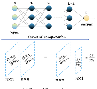
Figure 1: Gradient computation using forward propagation.

Like most optimization algorithms, the FW algorithm necessitates the computation of the gradient of the cost function. The calculation of the gradient in neural networks is typically performed using the forward propagation method, as illustrated in Fig. 1, or the backpropagation method, which reverses the computation process of the forward propagation. During forward propagation, determining the gradient involves the product of $L-1$ Jacobian matrices of order $m_{i}\times m_{i-1}$, where $m_{i}$ and $m_{i-1}$ denote the number of nodes at layers $i$ and $i-1$, respectively, and $L$ indicates the network’s depth. As such forward propropagation to compute the gradient is computationally expensive. In contrast, backpropagation circumvents this direct multiplication by initiating gradient computation from the output layer, propagating errors backward through the network. This technique, however, incurs a substantial memory overhead due to the necessity to retain these Jacobian matrices, the size of which is contingent upon the number of nodes in each layer and the overall depth of the network.

In scenarios with time-varying cost functions, using backpropagation or forward propagation for gradient computation in deep neural networks can be either infeasible or inefficient [7, 8]. As a result, recent works [9, 10, 11] have introduced the novel Projected Forward Gradient method as a solution. Illustrated in Fig 2, this technique significantly reduces the memory complexity associated with backpropagation while maintaining an equivalent level of computational expense. The Projected Forward Gradient is characterized as an unbiased estimate of the cost function’s gradient that can be calculated in a single forward pass of the network. Specifically, for a function $f:\mathbb{R}^{n}\rightarrow\mathbb{R}$, the Projected Forward Gradient $\boldsymbol{\mathbf{\phi}}(\boldsymbol{\mathbf{x}}):\mathbb{R}^{n}\rightarrow\mathbb{R}^{n}$ is expressed as $\boldsymbol{\mathbf{\phi}}(\boldsymbol{\mathbf{x}})=\langle\nabla f(\boldsymbol{\mathbf{x}}),\boldsymbol{\mathbf{u}}\rangle\boldsymbol{\mathbf{u}}$, where $\boldsymbol{\mathbf{u}}\in\mathbb{R}^{n}$ is a random vector with each entry $u_{i}$ being independent and identically distributed with zero mean and unit variance. The Projected Forward Gradient $\boldsymbol{\mathbf{\phi}}(\boldsymbol{\mathbf{x}})$ represents the directional derivative of the function $f(\boldsymbol{\mathbf{x}})$ along the random vector $\boldsymbol{\mathbf{u}}$, making it a computationally efficient and scalable method to train deep neural networks.

In this paper, we conduct a critical analysis of the application of the Projected Forward Gradient method within the FW optimization framework. We show that the direct employment of Projected Forward Gradient within the FW algorithm results in convergence to a neighborhood of the optimal solution, bounded away from optimality by an error margin inherently linked to the stochastic errors in the gradient approximation process. In light of this pivotal understanding, we introduce a second algorithm that innovatively averages historical projected gradient directions, thus effectively attenuating the stochastic noise. We establish, through rigorous proof, the favorable sublinear convergence rate to the optimal solution achieved by this algorithm. We demonstrate the convergence attributes of our proposed algorithms using a numerical example.

Our second algorithm, although inspired by momentum-based methods that are known to speed up the gradient descent algorithm [12], differs substantially in its implementation. Momentum-based techniques primarily use past gradients to accelerate convergence [13, 14, 15]. In contrast, our method takes a step further by incorporating the Projected Forward Gradient approach to reduce the inherent noise in gradient estimations systematically. This refined utilization of averaging historical Projected Forward Gradient directions sets it apart from conventional momentum methods, presenting a unique contribution that combines momentum principles with the strengths of Projected Forward Gradient to improve the convergence characteristics of the FW algorithm.

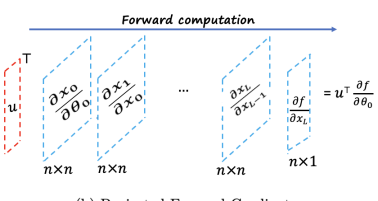
Figure 2: Projected Forward Gradient

The rest of the paper is organized as follows: in Section II, we review notations, definitions, basic assumptions, and background knowledge. In Section III, we discuss the problem setting. In Section III, we demonstrate that the Frank-Wolfe algorithm when provided access to the Projected Forward Gradient rather than the actual gradient, converges to a non-vanishing constant error bound. Moreover, in section III, we introduce the second algorithm and establish the sublinear convergence rate of the proposed algorithm to the optimal solution by utilizing the Projected Forward Gradient. In section V, we bring a numerical simulation which verify our theoretical founding. Finally, in Section VI, we conclude the paper.

II Notation and definitions

The set of real numbers is . For a vector $\boldsymbol{\mathbf{x}}\in{\mathbb{R}}^{n}$, we define the Euclidean and infinity norms by, respectively, $\|\boldsymbol{\mathbf{x}}\|\!=\!\sqrt{\boldsymbol{\mathbf{x}}^{\top}\boldsymbol{\mathbf{x}}}$ and $\|\boldsymbol{\mathbf{x}}\|_{\infty}\!=\!\max{|x_{i}|}_{i=1}^{n}$.

The partial derivative of a function $f(\boldsymbol{\mathbf{x}}):^{n}\rightarrow$ with respect to $\boldsymbol{\mathbf{x}}\in^{n}$ is given by $\nabla_{\boldsymbol{\mathbf{x}}}f(\boldsymbol{\mathbf{x}})$ (referred to hereafter as ‘gradient’). Also, $\nabla_{\boldsymbol{\mathbf{x}}\boldsymbol{\mathbf{x}}}f(\boldsymbol{\mathbf{x}})$ is the partial derivatives of $\nabla_{\boldsymbol{\mathbf{x}}}f(\boldsymbol{\mathbf{x}})$ with respect to $\boldsymbol{\mathbf{x}}$. A differentiable function $f:{\mathbb{R}}^{d}\to{\mathbb{R}}$ is $m$-strongly convex ($m\in_{>0}$) in ^d if and only if

$$(\boldsymbol{\mathbf{z}}-\boldsymbol{\mathbf{x}})\!^{\top}\!(\nabla f(\boldsymbol{\mathbf{z}})-\nabla f(\boldsymbol{\mathbf{x}}))\!\geq m\|\boldsymbol{\mathbf{z}}-\boldsymbol{\mathbf{x}}\|^{2},~{}~{}\forall\boldsymbol{\mathbf{x}},\boldsymbol{\mathbf{z}}\in\!^{d},~{}\boldsymbol{\mathbf{x}}\!\neq\!\boldsymbol{\mathbf{z}}.$$

For twice differentiable function $f$ the $m$-strong convexity is equivalent to $\nabla f(\boldsymbol{\mathbf{x}})\succeq m\boldsymbol{\mathbf{I}},~{}\forall~{}\boldsymbol{\mathbf{x}}\in^{d}.$ The gradient of a differentiable function $f:^{d}\to$ is globally Lipschitz with constant $M\in_{>0}$ (hereafter referred to simply as $M$-Lipschitz) if and only if

$$\left\|\nabla\boldsymbol{\mathbf{f}}(\boldsymbol{\mathbf{x}})-\nabla\boldsymbol{\mathbf{f}}(\boldsymbol{\mathbf{y}})\right\|\leq M\left\|\boldsymbol{\mathbf{x}}-\boldsymbol{\mathbf{y}}\right\|,\quad\forall\,\boldsymbol{\mathbf{x}},\boldsymbol{\mathbf{y}}\in^{d}.$$ (2)

For twice differentiable functions, condition (2) is equivalent to $\nabla_{\boldsymbol{\mathbf{x}}\boldsymbol{\mathbf{x}}}f(\boldsymbol{\mathbf{x}})\preceq M\boldsymbol{\mathbf{I}},~{}\forall~{}\boldsymbol{\mathbf{x}}\in^{d}$ [16]. A differentiable $m$-strongly function with a globally $M$-Lipschitz gradient for all $\boldsymbol{\mathbf{x}},\boldsymbol{\mathbf{y}}\in^{d}$ also satisfies [16]

$$\nabla f(\boldsymbol{\mathbf{x}})\!^{\top}\!(\boldsymbol{\mathbf{y}}-\boldsymbol{\mathbf{x}})+\frac{m}{2}\|\boldsymbol{\mathbf{y}}-\boldsymbol{\mathbf{x}}\|^{2}\leq f(\boldsymbol{\mathbf{y}})-f(\boldsymbol{\mathbf{x}})$$

$$\qquad\quad\quad\leq\nabla f(\boldsymbol{\mathbf{x}})^{\top}(\boldsymbol{\mathbf{y}}-\boldsymbol{\mathbf{x}})+\frac{M}{2}\|\boldsymbol{\mathbf{y}}-\boldsymbol{\mathbf{x}}\|^{2},$$ (3a)

$$\frac{1}{2M}\|\nabla f(\boldsymbol{\mathbf{x}})\|^{2}\leq f(\boldsymbol{\mathbf{x}})-f^{\star}\leq\frac{1}{2m}\|\nabla f(\boldsymbol{\mathbf{x}})\|^{2},$$ (3b)

where $f^{\star}$ is the minimum value of $f$.

III Objective Statement

In this paper we consider the optimization problem (1) where $f:^{n}\rightarrow$ is a smooth convex function and $\mathcal{C}\in^{n}$ is a compact convex set. We maintain the following assumptions throughout the paper about the cost function and constraint set of optimization problem (1).

Assumption 1 (Properties of the cost function).

The cost function $f(\boldsymbol{\mathbf{x}}):^{n}\rightarrow$ is twice continuously differentiable with respect to $\boldsymbol{\mathbf{x}}$. Moreover, the cost function has $M$-Lipschitz gradient in $\boldsymbol{\mathbf{x}}$, i.e., $\nabla_{\boldsymbol{\mathbf{x}}\boldsymbol{\mathbf{x}}}f(\boldsymbol{\mathbf{x}})\preceq M\,\boldsymbol{\mathbf{I}}_{n}.$ $\Box$

Assumption 2 (Properties of the constraint set $\mathcal{C}$).

The convex set $\mathcal{C}$ is bounded with diameter $D$, i.e., for all $x,y\in\mathcal{C}$ we have

$$\|x-y\|\leq D.$$ (4)

$\Box$

Algorithm 1 Frank-Wolf (FW) algorithm [5]

1:Require: $\alpha_{k}$

2:Input: $\boldsymbol{\mathbf{x}}_{0}\in\mathcal{C}$

3:Output: $\boldsymbol{\mathbf{x}}_{K+1}\in\mathcal{C}$

4:for $k=1,2,~{}...,K$ do

5:     Compute $\boldsymbol{\mathbf{s}}_{k}\in\operatorname{argmin}_{\boldsymbol{\mathbf{s}}\in\mathcal{C}}~{}{\boldsymbol{\mathbf{s}}^{\top}\nabla f(\boldsymbol{\mathbf{x}}_{k})}$

6:     $\boldsymbol{\mathbf{x}}_{k+1}=(1-\alpha_{k})\boldsymbol{\mathbf{x}}_{k}+\alpha_{k}\boldsymbol{\mathbf{s}}_{k}$

7:end for

Algorithm 1 demonstrates how the FW algorithm is applied to solve the optimization problem (1) [5]. In each iteration, the algorithm consults an oracle to identify the optimal point $\boldsymbol{\mathbf{s}}_{k}=\operatorname{argmin}_{\boldsymbol{\mathbf{s}}\in\mathcal{C}}~{}\boldsymbol{\mathbf{s}}^{\top}\nabla f(\boldsymbol{\mathbf{x}}_{k})$ by utilizing the linear approximation of the objective function $f$ at $\boldsymbol{\mathbf{x}}_{k}$. The process then involves updating the current solution to $\boldsymbol{\mathbf{x}}_{k+1}=(1-\alpha_{k})\boldsymbol{\mathbf{x}}_{k}+\alpha_{k}\boldsymbol{\mathbf{s}}_{k}$, where $\alpha_{k}\in[0,1]$ is a step size parameter. This adjustment ensures that $\boldsymbol{\mathbf{x}}_{k+1}$ remains feasible within the convex set $\mathcal{C}$, preserving the projection-free nature of the FW algorithm. The convergence of the FW algorithm is determined by a rate of $O(MD^{2}/k)$, where $D$ represents the diameter of $\mathcal{C}$ and $M$ is the smoothness constant of $f$.

The objective of this study is to enhance the memory efficiency of the FW algorithm in training deep neural networks by integrating Projected Forward Gradient. As mentioned in the Introduction section, for a function $f:\mathbb{R}^{n}\rightarrow\mathbb{R}$, the Projected Forward Gradient $\boldsymbol{\mathbf{\phi}}(\boldsymbol{\mathbf{x}}):\mathbb{R}^{n}\rightarrow\mathbb{R}^{n}$ is expressed as $\boldsymbol{\mathbf{\phi}}(\boldsymbol{\mathbf{x}})=\langle\nabla f(\boldsymbol{\mathbf{x}}),\boldsymbol{\mathbf{u}}\rangle\boldsymbol{\mathbf{u}}$, where $\boldsymbol{\mathbf{u}}\in\mathbb{R}^{n}$ is a random vector with each entry $u_{i}$ being independent and identically distributed with zero mean and unit variance. As outlined in the Introduction, Projected Forward Gradient computation avoids the conventionally dense matrix-matrix products seen in forward propagation by utilizing a vector transposed against the gradient, thereby reducing the multiplication to a less computationally expensive vector-matrix product (refer to Fig. 1 and Fig. 2 for visual comparison of forward propagation processes). The computational complexity of Projected Forward Gradient is thus analogous to the backpropagation algorithm, but notably, Projected Forward Gradient eschews the need for storing intermediate Jacobians–a step that is memory-intensive in backpropagation. These attributes render Projected Forward Gradient substantially more memory-efficient for gradient computation tasks. The Projected Forward Gradient Frank-Wolfe (FGFW) algorithm is presented in Algorithm 2.

In the following sections, we rigorously analyze the convergence behavior of Algorithm 2 and demonstrate that incorporating the Projected Forward Gradient induces a convergence error within the FW framework. To rectify this convergence discrepancy, we introduce a refined alternative algorithm that ensures exact convergence to the optimal solution while achieving a sublinear convergence rate.

IV Methods and Convergence Analysis

In this section, we study the convergence guarantee of Algorithm 2, which is designed based on using the Projected Forward Gradient estimator instead of the exact gradient within FW. Line 6 of Algorithm 2 corresponds to the Projected Forward Gradient. Following the computation of $\boldsymbol{\mathbf{u}}^{\prime}_{k}$, line 7 executes the linear programming step typical in FW. Finally, line 8 updates the decision variable. To facilitate our convergence analysis of Algorithm 2, we first review some auxiliary results about a property of the Projection Forward Gradient.

Lemma IV.1 (Upper bound on the Projected Forward Gradient [17]).

Let $\boldsymbol{\mathbf{u}}\in\mathbb{R}^{n}$ be a random vector with each entry $u_{i}$ being independent and identically distributed with zero mean and unit variance. Then the Projected Forward Gradient satisfies

$$\operatorname{\mathbb{E}}[\langle\boldsymbol{\mathbf{u}},\nabla f(\boldsymbol{\mathbf{x}})\rangle\boldsymbol{\mathbf{u}}]\leq(n+4)\|\nabla f(\boldsymbol{\mathbf{x}})\|^{2}.$$ (5)

$\Box$

The following result demonstrates that the Projected Forward Gradient is an unbiased estimation of $\nabla f(\boldsymbol{\mathbf{x}})$.

Lemma IV.2 (Unbiasedness of the Projected Forward Gradient estimator).

Let $\boldsymbol{\mathbf{u}}\in\mathbb{R}^{n}$ be a random vector with each entry $u_{i}$ being independent and identically distributed with zero mean and unit variance. Then, the Projected Forward Gradient estimator is an unbiased estimate of $\nabla f(\boldsymbol{\mathbf{x}})$.

Proof.

The proof follows from $\operatorname{\mathbb{E}}[\langle\boldsymbol{\mathbf{u}},\nabla f(\boldsymbol{\mathbf{x}})\rangle\boldsymbol{\mathbf{u}}]=\operatorname{\mathbb{E}}[\boldsymbol{\mathbf{u}}\boldsymbol{\mathbf{u^{\top}}}]\nabla f(\boldsymbol{\mathbf{x}})=\boldsymbol{\mathbf{I}}_{n}\nabla f(\boldsymbol{\mathbf{x}})=\nabla f(\boldsymbol{\mathbf{x}}),$ where we use the fact that a random vector $\boldsymbol{\mathbf{u}}$ and $\nabla f(\boldsymbol{\mathbf{x}})$ are independent of each other. ∎

With the auxiliary results at hand, we are now ready to present the convergence guarantee of Algorithm 2.

Algorithm 2 Forward Gradient Frank-Wolf (FGFW)

1:Require: $\alpha_{k}$

2:Input: $\boldsymbol{\mathbf{x}}_{0}\in\mathcal{C}$

3:Output: $\boldsymbol{\mathbf{x}}_{K+1}$

4:for $k=1,2,~{}...,K$ do

5:     Sample $\boldsymbol{\mathbf{u}}_{k}\sim\mathcal{N}(\boldsymbol{\mathbf{0}},\,\mathit{I}_{d}$)

6:     Compute $\boldsymbol{\mathbf{u}}_{k}^{\prime}=\langle\nabla f(\boldsymbol{\mathbf{x}}_{k}),\boldsymbol{\mathbf{u}}_{k}\rangle\boldsymbol{\mathbf{u}}_{k}$

7:     Compute $\boldsymbol{\mathbf{s}}_{k}\in\operatorname{argmin}_{\boldsymbol{\mathbf{s}}\in\mathcal{C}}~{}{\boldsymbol{\mathbf{s}}^{\top}\boldsymbol{\mathbf{u}}_{k}^{\prime}}$

8:     $\boldsymbol{\mathbf{x}}_{k+1}=(1-\alpha_{k})\boldsymbol{\mathbf{x}}_{k}+\alpha_{k}\boldsymbol{\mathbf{s}}_{k}$

9:end for

Theorem IV.1 (Convergence bound for Algorithm 2).

Consider optimizaiton problem (1) under Assumptions 1 and 2. Let $\gamma_{1}=MD^{2}\sqrt{n+4}$, $\gamma_{2}=\frac{MD^{2}}{2}$. Then, Algorithm 2 results in $\lim_{k\to\infty}\operatorname{\mathbb{E}}[f(\boldsymbol{\mathbf{x}}_{k})-f(\boldsymbol{\mathbf{x}}^{*})]$ to converge to $(\gamma_{1})$-neighborhood of the optimum solution with a sublinear convergence rate, i.e.,

$$\lim_{k\to\infty}\operatorname{\mathbb{E}}[f(\boldsymbol{\mathbf{x}}_{k})-f(\boldsymbol{\mathbf{x}}^{*})]\geq\gamma_{1}$$ (6)

Proof.

From Assumption 1, we have the following

$$\operatorname{\mathbb{E}}[f(\boldsymbol{\mathbf{x}}_{k+1})|\boldsymbol{\mathbf{x}}_{k}] \leq f(\boldsymbol{\mathbf{x}}_{k})+\big{\langle}\nabla f(\boldsymbol{\mathbf{x}}_{k}),\operatorname{\mathbb{E}}[\boldsymbol{\mathbf{x}}_{k+1}-\boldsymbol{\mathbf{x}}_{k}|\boldsymbol{\mathbf{x}}_{k}]\big{\rangle}$$

$$+\frac{M}{2}\operatorname{\mathbb{E}}\big{[}\|\boldsymbol{\mathbf{x}}_{k+1}-\boldsymbol{\mathbf{x}}_{k}\|^{2}\big{|}\boldsymbol{\mathbf{x}}_{k}\big{]},$$ (7)

substituting $\boldsymbol{\mathbf{x}}_{k+1}=(1-\alpha_{k})\boldsymbol{\mathbf{x}}_{k}+\alpha_{k}\boldsymbol{\mathbf{s}}_{k}$ in (IV) results in the following

$$\operatorname{\mathbb{E}}[f(\boldsymbol{\mathbf{x}}_{k+1})|\boldsymbol{\mathbf{x}}_{k}] \leq f(\boldsymbol{\mathbf{x}}_{k})+\alpha_{k}\langle\nabla f(\boldsymbol{\mathbf{x}}_{k}),\operatorname{\mathbb{E}}[\boldsymbol{\mathbf{s}}_{k}-\boldsymbol{\mathbf{x}}_{k}|\boldsymbol{\mathbf{x}}_{k}]\big{\rangle}$$

$$+\frac{M\alpha_{k}^{2}}{2}\operatorname{\mathbb{E}}\big{[}\|\boldsymbol{\mathbf{s}}_{k}-\boldsymbol{\mathbf{x}}_{k}\|^{2}\big{|}\boldsymbol{\mathbf{x}}_{k}\big{]},$$

$$=f(\boldsymbol{\mathbf{x}}_{k})+\alpha_{k}\langle\nabla f(\boldsymbol{\mathbf{x}}_{k})-\boldsymbol{\mathbf{u}}_{k}^{\prime},\operatorname{\mathbb{E}}[\boldsymbol{\mathbf{s}}_{k}-\boldsymbol{\mathbf{x}}_{k}|\boldsymbol{\mathbf{x}}_{k}]\big{\rangle}$$

$$+\alpha_{k}\langle\boldsymbol{\mathbf{u}}_{k}^{\prime},\operatorname{\mathbb{E}}[\boldsymbol{\mathbf{s}}_{k}-\boldsymbol{\mathbf{x}}_{k}|\boldsymbol{\mathbf{x}}_{k}]\big{\rangle}$$

$$+\frac{M\alpha_{k}^{2}}{2}\operatorname{\mathbb{E}}\big{[}\|\boldsymbol{\mathbf{s}}_{k}-\boldsymbol{\mathbf{x}}_{k}\|^{2}\big{|}\boldsymbol{\mathbf{x}}_{k}\big{]},$$ (8)

where we added and subtracted the term $\alpha_{k}\langle\boldsymbol{\mathbf{u}}_{k}^{\prime},\operatorname{\mathbb{E}}[\boldsymbol{\mathbf{s}}_{k}-\boldsymbol{\mathbf{x}}_{k}|\boldsymbol{\mathbf{x}}_{k}]\big{\rangle}$ in the last equality. Applying total expectation on both sides of (IV) we have

$$\operatorname{\mathbb{E}}[f(\boldsymbol{\mathbf{x}}_{k+1})] \leq\operatorname{\mathbb{E}}[f(\boldsymbol{\mathbf{x}}_{k})]+\alpha_{k}\operatorname{\mathbb{E}}[\langle\nabla f(\boldsymbol{\mathbf{x}}_{k})-\boldsymbol{\mathbf{u}}_{k}^{\prime},\boldsymbol{\mathbf{s}}_{k}-\boldsymbol{\mathbf{x}}_{k}\rangle]$$

$$+\alpha_{k}\operatorname{\mathbb{E}}[\langle\boldsymbol{\mathbf{u}}_{k}^{\prime},\boldsymbol{\mathbf{s}}_{k}-\boldsymbol{\mathbf{x}}_{k}\rangle]$$

$$+\frac{M\alpha_{k}^{2}}{2}\operatorname{\mathbb{E}}\big{[}\|\boldsymbol{\mathbf{s}}_{k}-\boldsymbol{\mathbf{x}}_{k}\|^{2}\big{]}$$

$$\leq\operatorname{\mathbb{E}}[f(\boldsymbol{\mathbf{x}}_{k})]+\alpha_{k}\operatorname{\mathbb{E}}[\langle\nabla f(\boldsymbol{\mathbf{x}}_{k})-\boldsymbol{\mathbf{u}}_{k}^{\prime},\boldsymbol{\mathbf{s}}_{k}-\boldsymbol{\mathbf{x}}_{k}\rangle]$$

$$+\alpha_{k}\operatorname{\mathbb{E}}[\langle\boldsymbol{\mathbf{u}}_{k}^{\prime},\boldsymbol{\mathbf{x^{*}}}-\boldsymbol{\mathbf{x}}_{k}\rangle]$$

$$+\frac{M\alpha_{k}^{2}}{2}\operatorname{\mathbb{E}}\big{[}\|\boldsymbol{\mathbf{s}}_{k}-\boldsymbol{\mathbf{x}}_{k}\|^{2}\big{]},$$ (9)

where in the last inequality, $\left\langle\boldsymbol{\mathbf{s}}_{k},\boldsymbol{\mathbf{u}}_{k}^{\prime}\right\rangle$ in (IV) is replaced by its upper bound $\left\langle\mathbf{x}^{*},\boldsymbol{\mathbf{u}}_{k}^{\prime}\right\rangle$ because $\left\langle\mathbf{x}^{*},\boldsymbol{\mathbf{u}}_{k}^{\prime}\right\rangle\geq\min_{\boldsymbol{\mathbf{s}}\in\mathcal{C}}\left\{\left\langle\boldsymbol{\mathbf{s}},\boldsymbol{\mathbf{u}}_{k}^{\prime}\right\rangle\right\}=\left\langle\boldsymbol{\mathbf{s}}_{k},\boldsymbol{\mathbf{u}}_{k}^{\prime}\right\rangle$. Adding and subtracting $\alpha_{k}\operatorname{\mathbb{E}}[\langle\nabla f(\boldsymbol{\mathbf{x}}_{k}),\boldsymbol{\mathbf{x}}^{*}-\boldsymbol{\mathbf{x}}_{k}\rangle]$ results in

$$\operatorname{\mathbb{E}}[f(\boldsymbol{\mathbf{x}}_{k+1})] \leq\operatorname{\mathbb{E}}[f(\boldsymbol{\mathbf{x}}_{k})]+\alpha_{k}\operatorname{\mathbb{E}}[\langle\nabla f(\boldsymbol{\mathbf{x}}_{k})-\boldsymbol{\mathbf{u}}_{k}^{\prime},\boldsymbol{\mathbf{s}}_{k}-\boldsymbol{\mathbf{x^{*}}}\rangle]$$

$$+\alpha_{k}\operatorname{\mathbb{E}}[\langle\nabla f(\boldsymbol{\mathbf{x}}_{k}),\boldsymbol{\mathbf{x^{*}}}-\boldsymbol{\mathbf{x}}_{k}\rangle]$$

$$+\frac{M\alpha_{k}^{2}}{2}\operatorname{\mathbb{E}}\big{[}\|\boldsymbol{\mathbf{s}}_{k}-\boldsymbol{\mathbf{x}}_{k}\|^{2}\big{]},$$ (10)

$$\leq\operatorname{\mathbb{E}}[f(\boldsymbol{\mathbf{x}}_{k})]+\alpha_{k}\operatorname{\mathbb{E}}[\langle\nabla f(\boldsymbol{\mathbf{x}}_{k})-\boldsymbol{\mathbf{u}}_{k}^{\prime},\boldsymbol{\mathbf{s}}_{k}-\boldsymbol{\mathbf{x^{*}}}\rangle]$$

$$+\alpha_{k}\operatorname{\mathbb{E}}[f(\boldsymbol{\mathbf{x}}^{*})-f(\boldsymbol{\mathbf{x}}_{k})]$$

$$+\frac{M\alpha_{k}^{2}}{2}\operatorname{\mathbb{E}}\big{[}\|\boldsymbol{\mathbf{s}}_{k}-\boldsymbol{\mathbf{x}}_{k}\|^{2}\big{]},$$ (11)

$$\leq\operatorname{\mathbb{E}}[f(\boldsymbol{\mathbf{x}}_{k})]+\alpha_{k}\operatorname{\mathbb{E}}[\|\nabla f(\boldsymbol{\mathbf{x}}_{k})-\boldsymbol{\mathbf{u}}_{k}^{\prime}\|\|\boldsymbol{\mathbf{s}}_{k}-\boldsymbol{\mathbf{x^{*}}}\|]$$

$$+\alpha_{k}\operatorname{\mathbb{E}}[f(\boldsymbol{\mathbf{x}}^{*})-f(\boldsymbol{\mathbf{x}}_{k})]$$

$$+\frac{M\alpha_{k}^{2}}{2}\operatorname{\mathbb{E}}\big{[}\|\boldsymbol{\mathbf{s}}_{k}-\boldsymbol{\mathbf{x}}_{k}\|^{2}\big{]},$$ (12)

where in the second and third inequality, we used the convexity property of the cost function $f$ (i.e., $f(\boldsymbol{\mathbf{x}}^{*})-f(\boldsymbol{\mathbf{x}}_{k})\geq\langle\nabla f(\boldsymbol{\mathbf{x}}_{k}),~{}\boldsymbol{\mathbf{x}}^{*}-\boldsymbol{\mathbf{x}}_{k}\rangle$) and Cauchy-Schwarz inequality, respectively. Invoking Assumption 2 we have

$$\operatorname{\mathbb{E}}[f(\boldsymbol{\mathbf{x}}_{k+1})] \leq\operatorname{\mathbb{E}}[f(\boldsymbol{\mathbf{x}}_{k})]+\alpha_{k}D\operatorname{\mathbb{E}}[\|\nabla f(\boldsymbol{\mathbf{x}}_{k})-\boldsymbol{\mathbf{u}}_{k}^{\prime}\|]$$

$$-\alpha_{k}\operatorname{\mathbb{E}}[f(\boldsymbol{\mathbf{x}}_{k})-f(\boldsymbol{\mathbf{x}}^{*})]+\frac{M\alpha_{k}^{2}D^{2}}{2},$$ (13)

adding and subtracting $f(\boldsymbol{\mathbf{x}}^{*})$ on the both sides we get

$$\operatorname{\mathbb{E}}[f(\boldsymbol{\mathbf{x}}_{k+1})-f(\boldsymbol{\mathbf{x}}^{*})] \leq(1-\alpha_{k})\operatorname{\mathbb{E}}[f(\boldsymbol{\mathbf{x}}_{k})-f(\boldsymbol{\mathbf{x}}^{*})]$$

$$+\alpha_{k}D\operatorname{\mathbb{E}}[\|\nabla f(\boldsymbol{\mathbf{x}}_{k})-\boldsymbol{\mathbf{u}}_{k}^{\prime}\|]+\frac{M\alpha_{k}^{2}D^{2}}{2}.$$

Invoking Lyapunov’s inequality, $(\mathbb{E}\|X\|^{r})^{1/r}\leq(\mathbb{E}\|X\|^{r^{\prime}})^{1/r^{\prime}}$ for $r=1,r^{\prime}=2$, we have

$$\operatorname{\mathbb{E}}[f(\boldsymbol{\mathbf{x}}_{k+1})-f(\boldsymbol{\mathbf{x}}^{*})] \leq(1-\alpha_{k})\operatorname{\mathbb{E}}[f(\boldsymbol{\mathbf{x}}_{k})-f(\boldsymbol{\mathbf{x}}^{*})]$$

$$+\alpha_{k}D\sqrt{\operatorname{\mathbb{E}}[\|\nabla f(\boldsymbol{\mathbf{x}}_{k})-\boldsymbol{\mathbf{u}}_{k}^{\prime}\|]^{2}}+\frac{M\alpha_{k}^{2}D^{2}}{2},$$

$$\leq(1-\alpha_{k})\operatorname{\mathbb{E}}[f(\boldsymbol{\mathbf{x}}_{k})-f(\boldsymbol{\mathbf{x}}^{*})]$$

$$+\alpha_{k}D\sqrt{\operatorname{\mathbb{E}}[\|\boldsymbol{\mathbf{u}}_{k}^{\prime}\|^{2}]}+\frac{M\alpha_{k}^{2}D^{2}}{2},$$ (14)

where in the last inequality we used the fact that $\operatorname{\mathbb{E}}[\|X-\operatorname{\mathbb{E}}[X]\|^{2}]=\operatorname{\mathbb{E}}[\|X\|^{2}]-\|\operatorname{\mathbb{E}}[X]\|^{2}\leq\operatorname{\mathbb{E}}[\|X\|^{2}]$.
Using Lemma 5 into (IV) we get

$$\operatorname{\mathbb{E}}[f(\boldsymbol{\mathbf{x}}_{k+1})-f(\boldsymbol{\mathbf{x}}^{*})] \leq(1-\alpha_{k})\operatorname{\mathbb{E}}[f(\boldsymbol{\mathbf{x}}_{k})-f(\boldsymbol{\mathbf{x}}^{*})]$$

$$+\alpha_{k}D\sqrt{(n+4)\|\nabla f(\boldsymbol{\mathbf{x}}_{k})\|^{2}}+\frac{M\alpha_{k}^{2}D^{2}}{2},$$ (15)

then, we have

$$\operatorname{\mathbb{E}}[f(\boldsymbol{\mathbf{x}}_{k+1})-f(\boldsymbol{\mathbf{x}}^{*})] \leq(1-\alpha_{k})\operatorname{\mathbb{E}}[f(\boldsymbol{\mathbf{x}}_{k})-f(\boldsymbol{\mathbf{x}}^{*})]$$

$$+\alpha_{k}MD^{2}\sqrt{n+4}+\frac{M\alpha_{k}^{2}D^{2}}{2}.$$ (16)

Next, define $\delta_{k+1}=\operatorname{\mathbb{E}}[f(\boldsymbol{\mathbf{x}}_{k+1})-f(\boldsymbol{\mathbf{x}}^{*})]$. Then, for all $k\geq 0$, we have

$$\delta_{k+1} \leq(1-\alpha_{k})\delta_{k}+\gamma_{1}\alpha_{k}+\gamma_{2}\alpha_{k}^{2},$$

where $\gamma_{1}=MD^{2}\sqrt{n+4}$ and $\gamma_{2}=\frac{MD^{2}}{2}$. Invoking Comparison Lemma and Lyapunov function, we proceed to complete the proof [18]. Consider $V_{k}=|\delta_{k}|$ as our candidate Lyapunov function. Then, we have

$$V_{k+1}-V_{k} =|(1-\alpha_{k})\delta_{k}+\alpha_{k}(\gamma_{1}+\gamma_{2}\alpha_{k})|-|\delta_{k}|$$

$$\leq-\alpha_{k}|\delta_{k}|+\alpha_{k}(\gamma_{1}+\gamma_{2}\alpha_{k})$$

$$=-\theta\alpha_{k}|\delta_{k}|-(1-\theta)\alpha_{k}|\delta_{k}|+\alpha_{k}(\gamma_{1}+\gamma_{2}\alpha_{k}),$$

where $0<\theta<1$. Then if $|\delta_{k}|\geq\frac{\gamma_{1}+\gamma_{2}\alpha_{k}}{1-\theta}$, we have exponentially convergence to the ball with radius $\frac{\gamma_{1}+\gamma_{2}\alpha_{k}}{1-\theta}$. Thus, we have

$$\lim_{k\to\infty}\operatorname{\mathbb{E}}[f(\boldsymbol{\mathbf{x}}_{k})-f(\boldsymbol{\mathbf{x}}^{*})]=\frac{\gamma_{1}}{1-\theta}\geq\gamma_{1},$$ (17)

with the rate determined by $O(\alpha_{k})$. ∎

According to the bound presented in (6), Algorithm 2 fails to achieve exact convergence, notably due to the inherent stochastic attributes of the Projected Forward Gradient. To rectify this non-deterministic limitation, we introduce Algorithm 3, which refines the convergence characteristic by aggregating historical Projected Forward Gradients. Specifically, line 7 in Algorithm 3 utilizes the mean of past Projected Forward Gradients, which systematically diminishes estimation variance. In what follows, we demonstrate this variance reduction mathematically, establishing that the variance of our averaged Projected Forward Gradient estimator asymptotically approaches zero, thereby ensuring exact convergence to the optimum. The theoretical groundwork supporting this assertion is articulated in the ensuing theorem and its proof. We proceed under the following assumption.

Assumption 3 (Assumption on bounded variance).

The Projected Forward Gradient estimator $\boldsymbol{\mathbf{\phi}}(\boldsymbol{\mathbf{x}})=\langle\nabla f(\boldsymbol{\mathbf{x}}),\boldsymbol{\mathbf{u}}\rangle\boldsymbol{\mathbf{u}}$ has a bounded variance, i.e., for all $\boldsymbol{\mathbf{x}}\in\mathcal{C}$ we have

$$\operatorname{\mathbb{E}}[\|\boldsymbol{\mathbf{\phi}}(\boldsymbol{\mathbf{x}})-\nabla f(\boldsymbol{\mathbf{x}})\|^{2}]\leq\mathsf{G}.$$ (18)

$\Box$

Algorithm 3 Averaged Forward Gradient Frank-Wolf (AFGFW)

1:Require: $\alpha_{k},\gamma_{k}$

2:Input: $\boldsymbol{\mathbf{x}}_{0}\in\mathcal{C},\boldsymbol{\mathbf{v}}_{0}=\boldsymbol{\mathbf{0}}$

3:Output: $\boldsymbol{\mathbf{x}}_{K+1}$

4:for $k=1,2,~{}...,K$ do

5:     Sample $\boldsymbol{\mathbf{u}}_{k}\sim\mathcal{N}(\boldsymbol{\mathbf{0}}_{d},\,\mathit{I}_{d})$

6:     Compute $\boldsymbol{\mathbf{u}}_{k}^{\prime}=\langle\nabla f(\boldsymbol{\mathbf{x}}_{k}),\boldsymbol{\mathbf{u}}_{k}\rangle\boldsymbol{\mathbf{u}}_{k}$

7:     Averaged forward gradient      $\boldsymbol{\mathbf{v}}_{k}=(1-\gamma_{k})\boldsymbol{\mathbf{v}}_{k-1}+\gamma_{k}\boldsymbol{\mathbf{u}}_{k}^{\prime}$

8:     Compute $\boldsymbol{\mathbf{s}}_{k}\in\operatorname{argmin}_{\boldsymbol{\mathbf{s}}\in\mathcal{C}}~{}{\boldsymbol{\mathbf{s}}^{\top}\boldsymbol{\mathbf{v}}_{k}}$

9:     $\boldsymbol{\mathbf{x}}_{k+1}=(1-\alpha_{k})\boldsymbol{\mathbf{x}}_{k}+\alpha_{k}\boldsymbol{\mathbf{s}}_{k}$

10:end for

Lemma IV.3 (The variance of the averaged Projected Forward Consider Gradient estimator converges to zero).

Consider optimizaiton problem (1) under Assumptions 1 and 2. If in Algorithm 3, we choose $\alpha_{k}$ and $\gamma_{k}$ such that $\lim_{k\to\infty}\frac{\alpha_{k}}{\gamma_{k}}=0$, then

$$\lim_{k\to\infty}\operatorname{\mathbb{E}}[\|\boldsymbol{\mathbf{v}}_{k}-\nabla f(\boldsymbol{\mathbf{x}}_{k})\|^{2}]=0,$$ (19)

with the rate determined by $\min\{O(\eta_{k}^{2})$, $O(\gamma_{k})\}$, where $\eta_{k}=\frac{\alpha_{k}}{\gamma_{k}}\in_{>0}$.

Proof.

Note that for $\boldsymbol{\mathbf{v}}_{k}$ generated by Algorithm 3, we have

$$\|\boldsymbol{\mathbf{v}}_{k}-\nabla f(\boldsymbol{\mathbf{x}}_{k})\|^{2} =\|(1-\gamma_{k})\boldsymbol{\mathbf{v}}_{k-1}+\gamma_{k}\boldsymbol{\mathbf{u}}^{\prime}_{k}-\nabla f(\boldsymbol{\mathbf{x}}_{k})\|^{2}$$

$$=\|(1-\gamma_{k})(\boldsymbol{\mathbf{v}}_{k-1}-\nabla f(\boldsymbol{\mathbf{x}}_{k}))$$

$$+\gamma_{k}(\boldsymbol{\mathbf{u}}^{\prime}_{k}-\nabla f(\boldsymbol{\mathbf{x}}_{k}))\|^{2}$$

$$=(1-\gamma_{k})^{2}\|(\boldsymbol{\mathbf{v}}_{k-1}-\nabla f(\boldsymbol{\mathbf{x}}_{k}))\|^{2}$$

$$+\gamma_{k}^{2}\|(\boldsymbol{\mathbf{u}}^{\prime}_{k}-\nabla f(\boldsymbol{\mathbf{x}}_{k}))\|^{2}$$

$$+2\gamma_{k}(1-\gamma_{k})(\boldsymbol{\mathbf{v}}_{k-1}-\nabla f(\boldsymbol{\mathbf{x}}_{k}))^{\top}$$

$$(\boldsymbol{\mathbf{u}}^{\prime}_{k}-\nabla f(\boldsymbol{\mathbf{x}}_{k}))$$

$$=(1-\gamma_{k})^{2}\|\boldsymbol{\mathbf{v}}_{k-1}-\nabla f(\boldsymbol{\mathbf{x}}_{k})$$

$$+\nabla f(\boldsymbol{\mathbf{x}}_{k-1})-\nabla f(\boldsymbol{\mathbf{x}}_{k-1})\|^{2}$$

$$+\gamma_{k}^{2}\|(\boldsymbol{\mathbf{u}}^{\prime}_{k}-\nabla f(\boldsymbol{\mathbf{x}}_{k}))\|^{2}$$

$$+2\gamma_{k}(1-\gamma_{k})(\boldsymbol{\mathbf{v}}_{k-1}-\nabla f(\boldsymbol{\mathbf{x}}_{k}))^{\top}$$

$$(\boldsymbol{\mathbf{u}}^{\prime}_{k}-\nabla f(\boldsymbol{\mathbf{x}}_{k})).$$ (20)

By taking conditional expectation on both sides of (IV), we have

$$\operatorname{\mathbb{E}}[\|\boldsymbol{\mathbf{v}}_{k}-\nabla f(\boldsymbol{\mathbf{x}}_{k})\|^{2} |\sigma_{k}]=(1-\gamma_{k})^{2}\operatorname{\mathbb{E}}[\|\boldsymbol{\mathbf{v}}_{k-1}-\nabla f(\boldsymbol{\mathbf{x}}_{k})$$

$$+\nabla f(\boldsymbol{\mathbf{x}}_{k-1})-\nabla f(\boldsymbol{\mathbf{x}}_{k-1})\|^{2}|\sigma_{k}]$$

$$+\gamma_{k}^{2}\operatorname{\mathbb{E}}[\|(\boldsymbol{\mathbf{u}}^{\prime}_{k}-\nabla f(\boldsymbol{\mathbf{x}}_{k}))\|^{2}|\sigma_{k}],$$ (21)

where $\sigma_{k}$ is a set that contains all the randomness up to iteration $k$. Expressing $\nabla f(\boldsymbol{\mathbf{x}}_{k-1})-\nabla f(\boldsymbol{\mathbf{x}}_{k})=\zeta_{k}\boldsymbol{\mathbf{p}}_{k}$ where $\boldsymbol{\mathbf{p}}_{k}$ is a normalized vector, i.e., $\|\boldsymbol{\mathbf{p}}_{k}\|=1$ and $\zeta_{k}\in_{>0}$ and $\lim_{k\to\infty}\zeta_{k}=0$ with the rate at least as $\alpha_{k}$ because of Lipschitzness of the gradient. Hence, if we choose $\alpha_{k}$ and $\gamma_{k}$ such that $\lim_{k\to\infty}\frac{\alpha_{k}}{\gamma_{k}}=0$. Then, we can write $\nabla f(\boldsymbol{\mathbf{x}}_{k-1})-\nabla f(\boldsymbol{\mathbf{x}}_{k})=\eta_{k}\gamma_{k}\boldsymbol{\mathbf{p}}_{k}$ where $\eta_{k}=\frac{\alpha_{k}}{\gamma_{k}}\in_{>0}$ and $\lim_{k\to\infty}\eta_{k}=0$. Lastly, taking total expectation on both sides of (IV), we have

$$\operatorname{\mathbb{E}}[\|\boldsymbol{\mathbf{v}}_{k}-\nabla f(\boldsymbol{\mathbf{x}}_{k})\|^{2}] =(1-\gamma_{k})^{2}\operatorname{\mathbb{E}}[\|\boldsymbol{\mathbf{v}}_{k-1}-\nabla f(\boldsymbol{\mathbf{x}}_{k-1})$$

$$+\eta_{k}\gamma_{k}\boldsymbol{\mathbf{p}}_{k}\|^{2}]$$

$$+\gamma_{k}^{2}\operatorname{\mathbb{E}}[\|(\boldsymbol{\mathbf{u}}^{\prime}_{k}-\nabla f(\boldsymbol{\mathbf{x}}_{k}))\|^{2}]$$

$$=(1-\gamma_{k})^{2}(1+\gamma_{k})^{2}\operatorname{\mathbb{E}}[\|\frac{1}{1+\gamma_{k}}\big{(}\boldsymbol{\mathbf{v}}_{k-1}$$

$$-\nabla f(\boldsymbol{\mathbf{x}}_{k-1})\big{)}+\frac{\gamma_{k}}{1+\gamma_{k}}\eta_{k}\boldsymbol{\mathbf{p}}_{k}\|^{2}]$$

$$+\gamma_{k}^{2}\operatorname{\mathbb{E}}[\|(\boldsymbol{\mathbf{u}}^{\prime}_{k}-\nabla f(\boldsymbol{\mathbf{x}}_{k}))\|^{2}].$$ (22)

Subsequently, invoking Jensen’s inequality, we have

$$\operatorname{\mathbb{E}}[\|\boldsymbol{\mathbf{v}}_{k}-\nabla f(\boldsymbol{\mathbf{x}}_{k})\|^{2}] \leq(1-\gamma_{k})^{2}(1+\gamma_{k})\operatorname{\mathbb{E}}[\|\boldsymbol{\mathbf{v}}_{k-1}-\nabla f(\boldsymbol{\mathbf{x}}_{k-1})\|^{2}]$$

$$+(1-\gamma_{k})^{2}(1+\gamma_{k})\gamma_{k}\eta_{k}^{2}$$

$$+\gamma_{k}^{2}\operatorname{\mathbb{E}}[\|(\boldsymbol{\mathbf{u}}^{\prime}_{k}-\nabla f(\boldsymbol{\mathbf{x}}_{k}))\|^{2}]$$

$$\leq(1-\gamma_{k})\operatorname{\mathbb{E}}[\|\boldsymbol{\mathbf{v}}_{k-1}-\nabla f(\boldsymbol{\mathbf{x}}_{k-1})\|^{2}]$$

$$+(1-\gamma_{k})\gamma_{k}\eta_{k}^{2}$$

$$+\gamma_{k}^{2}\operatorname{\mathbb{E}}[\|(\boldsymbol{\mathbf{u}}^{\prime}_{k}-\nabla f(\boldsymbol{\mathbf{x}}_{k}))\|^{2}]$$

$$\leq(1-\gamma_{k})\operatorname{\mathbb{E}}[\|\boldsymbol{\mathbf{v}}_{k-1}-\nabla f(\boldsymbol{\mathbf{x}}_{k-1})\|^{2}]$$

$$+\gamma_{k}\eta_{k}^{2}$$

$$+\gamma_{k}^{2}\operatorname{\mathbb{E}}[\|(\boldsymbol{\mathbf{u}}^{\prime}_{k}-\nabla f(\boldsymbol{\mathbf{x}}_{k}))\|^{2}],$$ (23)

where in the second inequality we used $(1-\gamma_{k})^{2}(1+\gamma_{k})=(1-\gamma_{k})(1-\gamma_{k}^{2})\leq(1-\gamma_{k})$ and the last inequlity comes from the fact that $(1-\gamma_{k})\leq 1$. Denoting $\delta_{k}=\operatorname{\mathbb{E}}[\|\boldsymbol{\mathbf{v}}_{k}-\nabla f(\boldsymbol{\mathbf{x}}_{k})\|^{2}]$ and invoking Assumption 3 in (IV), we have

$$\delta_{k} \leq(1-\gamma_{k})\delta_{k-1}+\gamma_{k}\eta_{k}^{2}+\gamma_{k}^{2}\mathsf{G}.$$ (24)

Invoking Comparison Lemma [18] and Lyapunov function, we proceed to complete the proof. Consider $V_{k-1}=|d_{k-1}|$ as our candidate Lyapunov function.

$$V_{k}-V_{k-1} =|(1-\gamma_{k})d_{k-1}+\gamma_{k}\eta_{k}^{2}+\gamma_{k}^{2}\mathsf{G}|-|d_{k-1}|$$

$$\leq-\gamma_{k}|d_{k-1}|+\gamma_{k}\eta_{k}^{2}+\gamma_{k}^{2}\mathsf{G}$$

$$=-\theta\gamma_{k}|d_{k-1}|-(1-\theta)\gamma_{k}|d_{k-1}|+\gamma_{k}\eta_{k}^{2}+\gamma_{k}^{2}\mathsf{G}$$

where $0<\theta<1$. Then if $|d_{k-1}|\geq\frac{\eta_{k}^{2}+\gamma_{k}\mathsf{G}}{(1-\theta)}$, we have exponentially convergence to the ball with radius $\frac{\eta_{k}^{2}+\gamma_{k}\mathsf{G}}{(1-\theta)}$. Then, the overall rate of the convergence of $\lim_{k\to\infty}\operatorname{\mathbb{E}}[\|\boldsymbol{\mathbf{v}}_{k}-\nabla f(\boldsymbol{\mathbf{x}}_{k})\|^{2}]=0$ is determined by $\min\{O(\eta_{k}^{2})$, $O(\gamma_{k})\}$. ∎

The convergence analysis of Algorithm 3 is presented in the next theorem.

Theorem IV.2 (Convergence analysis for Algorithm 3).

Consider Algorithm 3. Let Assumptions 1, 2 and 3 hold. Then, $\lim_{k\to\infty}\operatorname{\mathbb{E}}[f(\boldsymbol{\mathbf{x}}_{k})-f(\boldsymbol{\mathbf{x}}^{*})]\to 0$ with a sublinear convergence rate determined by $O(\frac{\alpha_{k}}{\gamma_{k}})$.

Proof.

Following the same procedure as in the proof of Theorem IV.1, we obtain

$$\mathbb{E}[f(\mathbf{x}_{k+1})-f(\mathbf{x}^{*})] \leq(1-\alpha_{k})\mathbb{E}[f(\mathbf{x}_{k})-f(\mathbf{x}^{*})]$$

$$\quad+\alpha_{k}D\sqrt{\mathbb{E}[\|\nabla f(\mathbf{x}_{k})-\mathbf{v}_{k}\|^{2}]}+\frac{M\alpha_{k}^{2}D^{2}}{2},$$

Next, define $\delta_{k+1}=\operatorname{\mathbb{E}}[f(\boldsymbol{\mathbf{x}}_{k+1})-f(\boldsymbol{\mathbf{x}}^{*})]$. Then, we have

$$\delta_{k+1} \leq(1-\alpha_{k})\delta_{k}+\gamma_{1}\alpha_{k}+\gamma_{2}\alpha_{k}^{2},\quad\forall k\geq 0$$ (25)

where $\gamma_{1}=D\sqrt{\operatorname{\mathbb{E}}[\|\nabla f(\boldsymbol{\mathbf{x}}_{k})-\boldsymbol{\mathbf{v}}_{k}\|]^{2}}$ and $\gamma_{2}=\frac{MD^{2}}{2}$. Same as the proof in theorem IV.1, choosing $V_{k}=|\delta_{k}|$ as our candidate Lyapunov function, we obtain

$$V_{k+1}-V_{k} \leq-\theta\alpha_{k}|\delta_{k}|-(1-\theta)\alpha_{k}|\delta_{k}|+\alpha_{k}(\gamma_{1}+\gamma_{2}\alpha_{k}),$$

where $0<\theta<1$. Then if $|\delta_{k}|\geq\frac{\gamma_{1}+\gamma_{2}\alpha_{k}}{1-\theta}$, we have exponentially convergence to the ball with radius $\frac{\gamma_{1}+\gamma_{2}\alpha_{k}}{1-\theta}$. Hence, using Lemma IV.3, the overall rate of convergence of $\lim_{k\to\infty}\operatorname{\mathbb{E}}[f(\boldsymbol{\mathbf{x}}_{k})-f(\boldsymbol{\mathbf{x}}^{*})]=0$ is determined by $O(\frac{\alpha_{k}}{\gamma_{k}})$. ∎

V Illustrative Numerical Simulations

In this section, we demonstrate the convergence performance of Algorithm 2 and Algorithm 3 on the sparse multinomial logistic regression problem. The problem of interest is to solve the sparse multinomial logistic regression problem for recognizing the handwritten digits 0 to 9 from the MNIST dataset [19]. $\ell_{1}$-norm is used to produce the sparsity constraint, i.e., we seek to optimize the following

$$\min_{\theta} -\frac{1}{m}\left[\sum_{i=1}^{m}\sum_{j=1}^{k}\boldsymbol{\mathbf{1}}\left\{y^{(i)}=j\right\}\log\frac{\exp\left(\theta_{j}^{T}x^{(i)}\right)}{\sum_{1\leq i\leq k}\exp\left(\theta_{l}^{T}x^{(i)}\right)}\right]$$

s.t. $$\quad\|{\theta_{j}}\|_{1}\leqslant 1,\quad\forall j\in\{1,2,...,k\}.$$

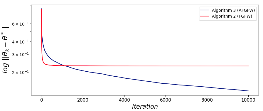
Figure 3: log error of the performance of Algorithm 2 versus Algorithm 3,

where $m=70000$ is the number of training instances, and $k=10$ denotes the number of classes corresponding to each digit. To implement Algorithms 2 and 3, we choose $\gamma_{k}=\frac{1}{\sqrt{k}}$ and $\alpha_{k}=\frac{1}{k}$. Figure 3 shows the mean of 50 Monte Carlo runs. As demonstrated in Theorem IV.1, Algorithm 2 converges to the steady-state error bound exponentially fast, which explains the rapid behavior of Algorithm 2 at the beginning of the process. In contrast, Algorithm 3 decays and eventually reaches the optimal solution with a sublinear rate of converges proved in Theorem IV.2.

VI Conclusion

In this paper, we analyzed the performance of the FW algorithm when a Projected Forward Gradient is used in place of exact gradient. Our results showed that trivial implementation of the projected forward gradient introduces a nonzero convergence error for the FW algorithm. To remove the converegnce errir, we presented Algorithm 3, an advancement of the Frank-Wolfe optimization technique, which uniquely incorporates the Projected Forward Gradient to systematically reduce noise in gradient estimations and ensure exact convergence to a proximal error bound of the optimal solution at a sublinear rate. The effectiveness of this algorithm was substantiated through rigorous proof and demonstrated numerically with logistic regression applied to the MNIST dataset. Our work offers significant computational and memory efficiency benefits in training high-dimensional deep neural networks. Future endeavors will focus on adapting the proposed methods to dynamic environments and exploring their potential in distributed settings that align with network topologies

References

- [1] I. Goodfellow, Y. Bengio, and A. Courville, “Deep learning,” 2016.
- [2] I. Goodfellow, Y. Bengio, and A. Courville, Deep learning. 2016.
- [3] M. Rostami and S. S. Kia, “Federated learning using variance reduced stochastic gradient for probabilistically activated agents,” in 2023 American Control Conference (ACC), pp. 861–866, IEEE, 2023.
- [4] E. Hazan and S. Kale, “Projection-free online learning,” arXiv preprint arXiv:1206.4657, 2012.
- [5] M. Frank, P. Wolfe, et al., “An algorithm for quadratic programming,” Naval research logistics quarterly, vol. 3, no. 1-2, pp. 95–110, 1956.
- [6] S. N. Ravi, T. Dinh, V. Lokhande, and V. Singh, “Constrained deep learning using conditional gradient and applications in computer vision,” arXiv preprint arXiv:1803.06453, 2018.
- [7] M. Rostami, H. Moradian, and S. Kia, “First-order dynamic optimization for streaming convex costs,” arXiv preprint arXiv:2310.07925, 2023.
- [8] M. Fazlyab, S. Paternain, and A. Ribeiro, “Prediction-correction interior-point method for time-varying convex optimization,” IEEE Transactions on Automatic Control, vol. 63, no. 7, pp. 1973–1986, 2017.
- [9] D. Silver, A. Goyal, I. Danihelka, M. Hessel, and H. van Hasselt, “Learning by directional gradient descent,” in International Conference on Learning Representations, 2022.
- [10] A. G. Baydin, B. A. Pearlmutter, D. Syme, F. Wood, and P. Torr, “Gradients without backpropagation,” arXiv preprint arXiv:2202.08587, 2022.
- [11] D. Krylov, A. Karamzade, and R. Fox, “Moonwalk: Inverse-forward differentiation,” arXiv preprint arXiv:2402.14212, 2024.
- [12] N. Qian, “On the momentum term in gradient descent learning algorithms,” Neural networks, vol. 12, no. 1, pp. 145–151, 1999.
- [13] C. Liu and M. Belkin, “Accelerating SGD with momentum for over-parameterized learning,” arXiv preprint arXiv:1810.13395, 2018.
- [14] W. Liu, L. Chen, Y. Chen, and W. Zhang, “Accelerating federated learning via momentum gradient descent,” IEEE Transactions on Parallel and Distributed Systems, vol. 31, no. 8, pp. 1754–1766, 2020.
- [15] G. Nakerst, J. Brennan, and M. Haque, “Gradient descent with momentum—to accelerate or to super-accelerate?,” arXiv preprint arXiv:2001.06472, 2020.
- [16] Y. Nesterov, Lectures on convex optimization, vol. 137. Springer, 2018.
- [17] Y. Nesterov and V. Spokoiny, “Random gradient-free minimization of convex functions,” Foundations of Computational Mathematics, vol. 17, pp. 527–566, 2017.
- [18] H. K. Khalil, Nonlinear Systems. Englewood Cliffs, NJ: Prentice Hall, 3 ed., 2002.
- [19] L. Deng, “The mnist database of handwritten digit images for machine learning research,” IEEE Signal Processing Magazine, vol. 29, no. 6, pp. 141–142, 2012.