FairSIN: Achieving Fairness in Graph Neural Networks
through Sensitive Information Neutralization

Abstract

Despite the remarkable success of graph neural networks (GNNs) in modeling graph-structured data, like other machine learning models, GNNs are also susceptible to making biased predictions based on sensitive attributes, such as race and gender. For fairness consideration, recent state-of-the-art (SOTA) methods propose to filter out sensitive information from inputs or representations, e.g., edge dropping or feature masking. However, we argue that such filtering-based strategies may also filter out some non-sensitive feature information, leading to a sub-optimal trade-off between predictive performance and fairness. To address this issue, we unveil an innovative neutralization-based paradigm, where additional Fairness-facilitating Features (F3) are incorporated into node features or representations before message passing. The F3 are expected to statistically neutralize the sensitive bias in node representations and provide additional non-sensitive information. We also provide theoretical explanations for our rationale, concluding that F3 can be realized by emphasizing the features of each node’s heterogeneous neighbors (neighbors with different sensitive attributes). We name our method as FairSIN, and present three implementation variants from both data-centric and model-centric perspectives. Experimental results on five benchmark datasets with three different GNN backbones show that FairSIN significantly improves fairness metrics while maintaining high prediction accuracies. Codes and appendix can be found at https://github.com/BUPT-GAMMA/FariSIN.

1 Introduction

Graph neural networks (GNNs) have shown their strong ability in modeling structured data, and are widely used in a variety of applications, e.g., e-commerce (Li et al. 2020; Niu et al. 2020) and drug discovery (Xiong et al. 2021; Bongini, Bianchini, and Scarselli 2021). Nevertheless, recent studies (Agarwal, Lakkaraju, and Zitnik 2021; Dai and Wang 2021; Chen et al. 2021; Shumovskaia et al. 2021; Li et al. 2021) show that the predictions of GNNs could be biased towards some demographic groups defined by sensitive attributes, e.g., race (Agarwal, Lakkaraju, and Zitnik 2021) and gender (Lambrecht and Tucker 2019). In decision-critical applications such as Credit evaluation (Yeh and Lien 2009), the discriminatory predictions made by GNNs may bring about severe societal concerns.

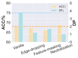
(a)

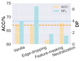
(b)

Figure 1: Motivation verification on Pokec datasets. Compared with vanilla GNN without fairness consideration, filtering-based methods, either edge-dropping (Agarwal, Lakkaraju, and Zitnik 2021) or feature-masking (Wang et al. 2022c), always have a trade-off between accuracy (ACC$\uparrow$) and fairness (DP$\downarrow$). While our method can improve both.

Generally, the biases in GNN predictions can be attributed to both node features and graph topology: (1) The raw features of nodes could be statistically correlated to the sensitive attribute, and thus lead to sensitive information leakage in encoded representations. (2) According to the homophily effects (McPherson, Smith-Lovin, and Cook 2001; La Fond and Neville 2010), nodes with the same sensitive attribute tend to link with each other, which will make the node representations in the same sensitive group more similar during message passing.

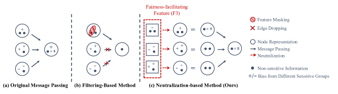
Figure 2: Motivation illustration of sensitive information neutralization. Here we assume binary sensitive groups denoted by +/-, and the numbers of +/- indicate the intensity of sensitive information leakage in node representations. (a) Message passing computation will aggregate both non-sensitive feature information (dot symbols) and sensitive biases (+/- symbols); (b) Current SOTA methods are usually filtering-based (e.g., edge dropping or feature masking), which may lose much non-sensitive information; (c) Our proposed neutralization-based strategy introduces F3 to statistically neutralize the sensitive bias and provide extra non-sensitive information.

To address the issue of sensitive biases, researchers have introduced fairness considerations into GNNs (Agarwal, Lakkaraju, and Zitnik 2021; Dai and Wang 2021; Bose and Hamilton 2019; Wang et al. 2022c; Dong et al. 2022a). Recent state-of-the-art (SOTA) methods often attempt to mitigate the impact of sensitive information by applying heuristic or adversarial constraints to filter it out from inputs or representations. For instance, NIFTY (Agarwal, Lakkaraju, and Zitnik 2021) employs counterfactual regularizations to perturb node features and drop edges. FairVGNN (Wang et al. 2022c), aided by adversarial discriminators, learns adaptive representation masks to exclude sensitive-relevant information. Nevertheless, as depicted in Figure 1 and  2(b), we contend that such filtering-based strategies may also filter out some non-sensitive feature information, leading to a sub-optimal balance between accuracy and fairness.

In light of this, we propose an alternative neutralization-based paradigm, as shown in Figure 2(c). The core idea is to introduce extra Fairness-facilitating Features (F3) to node features or representations so that the sensitive biases (+/- symbols) can be neutralized. The F3 are also expected to provide additional non-sensitive feature information (dot symbols), thus enabling a better trade-off between predictive performance and fairness. Specifically, we show how message passing exacerbates sensitive biases, and accordingly conclude that node features or representations can be debiased before message passing by emphasizing the features of each node’s heterogeneous neighbors (neighbors with different sensitive attributes) as F3. But some nodes in real-world graphs have very few or even no heterogeneous neighbors, which makes the calculation of F3 infeasible or very uncertain. Therefore, we propose to train an estimator to predict the average features or representations of a node’s heterogeneous neighbors given its own feature. In this way, nodes with rich heterogeneous neighbors can transfer their knowledge to other nodes through the estimator. We name our method as FairSIN, and further present three implementation variants from both data-centric and model-centric perspectives. Experimental results on five benchmark datasets with three different GNN backbones demonstrate the motivation and effectiveness of our proposed method.

Our contributions are as follows: (1) We present a novel neutralization-based paradigm for learning fair GNNs, which introduces Fairness-facilitating Features (F3) to node features/representations for debiasing sensitive attributes and providing additional non-sensitive information. (2) We show that F3 can be implemented by emphasizing the features of each node’s heterogeneous neighbors, and further propose three effective variants of FairSIN. (3) Experimental results show that the proposed FairSIN can reach a better trade-off between predictive performance and fairness compared with recent SOTA methods.

2 Related Work

Graph Neural Networks.

Graph-structured data widely exists in various real-world applications. To handle this type of non-Euclidean data, graph neural networks are designed for representation learning of nodes/edges/graphs, enabling a wide range of downstream tasks. For example, Graph Convolutional Network (GCN) (Kipf and Welling 2017) uses convolutional operations to perform layer-by-layer abstraction and refinement of node features. Graph Isomorphism Network (GIN) (Xu et al. 2019) is a method proposed to have more discriminative power for graph structures and make GNN as powerful as WL-test (Shervashidze et al. 2011). GraphSAGE (Hamilton, Ying, and Leskovec 2017) is an inductive representation learning method that can be used for large-scale data, and Graph Attention Network (GAT) (Veličković et al. 2018) is an attention-based method that assigns different weights to different neighbors during message passing. These methods have shown outstanding performance in various graph-based applications.

Fairness in Graph Neural Networks.

Fairness issues in machine learning models have gained increasing attention from both academia (Dong et al. 2023; Chouldechova and Roth 2018; Sun et al. 2019; Mehrabi et al. 2021; Field et al. 2021) and industry (Holstein et al. 2019). In terms of GNNs, there are different fairness definitions proposed in the literature (Dwork et al. 2012; Hardt, Price, and Srebro 2016; Dong et al. 2021; Kusner et al. 2017; Kang et al. 2022; Wang et al. 2022b). Among them, group fairness is one of the most popular notion (Dwork et al. 2012; Hardt, Price, and Srebro 2016), which aims at providing equal predictions for all demographic groups without any biases or discrimination. Due to the presence of sensitive-relevant features, GNNs may inadvertently perpetuate or amplify biases and discrimination against certain sensitive groups.

Improving group fairness in GNNs has attracted much attention over the last five years (Li et al. 2021; Bose and Hamilton 2019; Dong et al. 2023; Rahman et al. 2019; Laclau et al. 2021; Fisher et al. 2020). Recent SOTA methods usually employ feature masking or topology modification to filter out sensitive biases during message passing. For feature masking, (Bose and Hamilton 2019) leverages adversarial learning to enforce compositional fairness constraints on graph embeddings for multiple sensitive attributes filtering. FairVGNN (Wang et al. 2022c) uses a mask generator to filter out channels with high correlation to sensitive attributes. While others have investigated how to drop edges with high bias (Dong et al. 2022b; Spinelli et al. 2021). For example, REFEREE (Dong et al. 2022b) provides structural explanations of topology bias on how to improve fairness. FairDrop (Spinelli et al. 2021) adopts edge masking to counter-act homophily. It is worth noting that some methods (Dong et al. 2022a; Ling et al. 2023) not only drop edges but also add new ones. However, considering the addition of new edges has to compute the similarity between all node pairs that are not connected, thus introducing a time and space complexity of $\mathcal{O}(n^{2})$. This could be computationally expensive and thus edge dropping is a more practical choice. Also, some methods consider both feature masking and topology modification (Dong et al. 2022a; Ling et al. 2023; Kose and Shen 2022). Such filtering-based methods based on feature masking or edge dropping will unavoidably lead to the loss of useful non-sensitive information. Therefore, we propose a novel neutralization-based method that introduces F3 to statistically neutralize the sensitive bias and provide extra non-sensitive information.

3 Methodology

In this section, we will elaborate on the details of our proposed FairSIN, which employs the features/representations of heterogeneous neighbors to simultaneously neutralize sensitive biases and incorporate extra non-sensitive information.

3.1 Preliminaries

Notations.

Let $\mathcal{G}=(\mathcal{V},\mathcal{E})$ be a graph with node set $\mathcal{V}$ and edge set $\mathcal{E}$. The adjacency matrix $\mathbf{A}\in\mathbb{R}^{|\mathcal{V}|\times|\mathcal{V}|}$ represents the connectivity between nodes, where $\mathbf{A}_{ij}=1$ if there is a directed edge between nodes $v_{i}$ and $v_{j}$, and $\mathbf{A}_{ij}=0$ otherwise. The node feature matrix $\mathbf{X}\in\mathbb{R}^{|\mathcal{V}|\times d}$ contains the feature vectors for each node, where $\mathbf{x}_{i}\in\mathbb{R}^{d}$ is the feature vector for node $v_{i}\in\mathcal{V}$. Besides, each node $v_{i}$ also has a categorical sensitive attribute $s_{i}\in\mathcal{S}$.

Task Definition.

In this paper, we consider the benchmark task as previous work (Wang et al. 2022c; Agarwal, Lakkaraju, and Zitnik 2021; Dai and Wang 2021) did, i.e., the semi-supervised node classification task. Formally, given graph $\mathcal{G}$, node features $\mathbf{X}$ and labeled node set $\mathcal{V}^{L}\subset\mathcal{V}$, we need to build a model to predict the label $\hat{y}\in\mathcal{Y}$ for every node in the unlabeled node set $\mathcal{V}^{U}=\mathcal{V}\setminus\mathcal{V}^{L}$. A typical design of the model is to combine a GNN encoder and a classifier. The classification performance can be measured by aligning the ground truth labels $Y$ and predicted ones $\hat{Y}$. In terms of fairness, the goal is to weaken the dependency level between predicted labels $\hat{Y}$ and sensitive attributes $S$, without losing much classification accuracy. In practice, many fair representation learning methods  (Edwards and Storkey 2015; Dai and Wang 2021; Bose and Hamilton 2019; Liao et al. 2019) will minimize the dependency between node representations and sensitive attributes instead.

3.2 Theoretical Analysis

In this subsection, we will introduce our motivation of neutralizing sensitive information from a theoretical perspective. Firstly, we treat node features and graph topology as random variables, and describe a generative process to model the dependency among them. Similar generative process has been done in (Wang et al. 2022a). Then we propose to measure the sensitive information leakage by the conditional entropy between sensitive attributes and node representations. Finally, we show how the message passing computation exacerbates the leakage problem of sensitive information. Note that there is a slight abuse of notations about random variables and samples in this subsection.

Generative Process.

Here we describe a graph generation process with the following two steps: (1) For each node $v_{i}$, we draw its features and sensitive attribute from a joint prior distribution $(x_{i},s_{i})\sim\textit{prior}$. For simplicity, we assume that the sensitive attribute is binary as previous work did (Wang et al. 2022c; Agarwal, Lakkaraju, and Zitnik 2021; Dai and Wang 2021), and use $\bar{s}$ to denote the opposite counterpart of $s$. (2) To obtain graph $\mathcal{G}$, each node $v_{i}$ samples its in-degree neighbor set $\mathcal{N}_{i}$ by the homophily assumption(McPherson, Smith-Lovin, and Cook 2001; Wang et al. 2022a), where nodes with similar features or sensitive attributes are more likely to get connected. We name the neighbors with same/different sensitive attributes as homogeneous/heterogeneous neighbors, respectively.

We use $P_{i}^{\textit{same}}$/$P_{i}^{\textit{diff}}$ to represent the probability that $v_{i}$ samples a homogeneous/heterogeneous neighbor. According to the homophily assumption, $P_{i}^{\textit{same}}>P_{i}^{\textit{diff}}$. Then we denote the average feature of $v_{i}$’s in-degree neighbors as $x_{i}^{\textit{neigh}}$. The average features of $v_{i}$’s homogeneous/heterogeneous in-degree neighbors are written as $x_{i}^{\textit{same}}$/$x_{i}^{\textit{diff}}$. Thus $x_{i}^{\textit{neigh}}=P_{i}^{\textit{same}}x_{i}^{\textit{same}}+P_{i}^{\textit{diff}}x_{i}^{\textit{diff}}$.

Quantifying Sensitive Information Leakage.

In this work, we focus on alleviating sensitive biases in node representations, and use the conditional entropy between sensitive attributes and node representations as the measurement. Without loss of generality, we take raw features $x$ as node representations, and compute the conditional entropy as

$$\mathcal{H}(s|x)=-\mathbb{E}_{(x,s)\sim prior}\log P(s|x),$$ (1)

where $P(s|x)$ is a predictor that estimates sensitive attributes given node representations. When node representations have more sensitive information leakage, the predictor will be more accurate and the entropy will get smaller.

In practical applications, it becomes necessary to approximate the ground truth predictor $P(s|x)$. Specifically, we adopt a linear intensity function $\mathcal{D}_{\theta}$ with the parameter $\theta$ to define the predictive capability, satisfying the conditions: $\mathcal{D}_{\theta}(s|x)\sim\mathcal{N}(\mu_{c},\sigma^{2})$ and $\mathcal{D}_{\theta}(\bar{s}|x)\sim\mathcal{N}(\mu_{ic},\sigma^{2})$, where $(x,s)\sim\textit{prior}$ and $\mathcal{N}(\cdot,\cdot)$ is the Gaussian distribution. $\mu_{c}>\mu_{ic}$ indicates that $\mathcal{D}_{\theta}$ is more likely to assign larger intensity score to the true sensitive attribute given node representations. The larger $\mu_{c}-\mu_{ic}$ is, the stronger the inference capability of $\mathcal{D}_{\theta}$. In contrast, $\mu_{c}=\mu_{ic}$ means that $\mathcal{D}_{\theta}$ can not distinguish the sensitive attribute from representations.

Then we can define the parameterized predictor $\hat{P}_{\theta}(s|x)$ by normalizing the intensity function $\mathcal{D}_{\theta}$.

Message Passing Can Exacerbate Sensitive Biases.

Now we will straightforwardly provide an exposition from the perspective of sensitive information neutralization that the message passing computation may lead to more serious sensitive information leakage problem.

Theorem 1.

Assume that node representations are biased and can be identified by the predictor, i.e., $\mu_{c}>\mu_{ic}$. For node $v_{i}$, we consider a message passing process that updates $x_{i}$ by $x_{i}^{\prime}=x_{i}+x_{i}^{\textit{neigh}}$. Then we have

$$\mathbb{E}\{\mathcal{D}_{\theta}(s_{i}|x_{i}^{\prime})-\mathcal{D}_{\theta}(\bar{s_{i}}|x_{i}^{\prime})\}>\mathbb{E}\{\mathcal{D}_{\theta}(s_{i}|x_{i})-\mathcal{D}_{\theta}(\bar{s_{i}}|x_{i})\},$$ (2)

which means that the predictor $\hat{P}_{\theta}$ can identify the sensitive attributes more accurately.

The details and the proof of Theorem 1 can be found in the Appendix.

Summary.

Therefore, to alleviate the sensitive biases, we can either modify the graph structure to decrease $P_{i}^{\textit{same}}-P_{i}^{\textit{diff}}$ or modify the node features before message passing to decrease $\mu_{c}-\mu_{ic}$. Both solutions actually emphasize the features of each node’s heterogeneous neighbors, and can be seen as introducing extra F3 into node representations for sensitive information neutralization.

3.3 Implementations of FairSIN

Inspired by the above motivation, we will present three implementation variants from both data-centric and model-centric perspectives. We name our method as Fair GNNs via Sensitive Information Neutralization (FairSIN).

Data-centric Variants.

For data-centric implementation, we will employ a pre-processing manner, and modify the graph structure or node features before the training of GNN encoder.

(1) In terms of graph modification, we can simply change the edge weights in the adjacency matrix:

$$\mathbf{A}_{ij}=\begin{cases}\quad 1+\delta,\quad\text{if $(v_{i},v_{j})\in\mathcal{E}$ and $s_{i}\neq s_{j}$}\\ \quad 1,\quad\quad\;\;\text{if $(v_{i},v_{j})\in\mathcal{E}$ and $s_{i}=s_{j}$}\\ \quad 0,\quad\quad\;\;\text{if $(v_{i},v_{j})\not\in\mathcal{E}$}\\ \end{cases},$$ (3)

where $\delta>0$ is a hyper-parameter. We name this variant as FairSIN-G.

(2) In terms of feature modification, we first compute the average feature of each node $v_{i}$’s heterogeneous neighbors as $\mathbf{x}_{i}^{\textit{diff}}=\frac{1}{|\mathcal{N}_{i}^{\textit{diff}}|}\sum_{v_{j}\in\mathcal{N}_{i}^{\textit{diff}}}\mathbf{x}_{j}$, where $\mathcal{N}_{i}^{\textit{diff}}$ is the heterogeneous neighbor set of $v_{i}$. Here $\mathbf{x}_{i}^{\textit{diff}}$ can also be seen as the expectation estimation of the random variable ${x}_{i}^{\textit{diff}}$ defined in previous subsection.

However, some nodes in real-world graphs have very few or even no heterogeneous neighbors, which makes the calculation of $\mathbf{x}_{i}^{\textit{diff}}$ infeasible or very uncertain. To address this issue, we propose to train a multi-layer perceptron (MLP) to estimate $\mathbf{x}_{i}^{\textit{diff}}$:

$$\mathcal{L}_{F}=\frac{1}{|\mathcal{V}|}\sum_{i:|\mathcal{N}_{i}^{\textit{diff}}|\geq 1}\|\operatorname{MLP}_{\phi}(\mathbf{x}_{i})-\mathbf{x}_{i}^{\textit{diff}}\|^{2}.$$ (4)

By minimizing the above Mean Squared Error (MSE) loss, nodes with rich heterogeneous neighbors can transfer their knowledge to other nodes through the MLP. Then we neutralize each node $v_{i}$’s feature as $\tilde{\mathbf{x}}_{i}=\mathbf{x}_{i}+\delta\operatorname{MLP}_{\phi}(\mathbf{x}_{i})$, and name this variant as FairSIN-F.

Model-centric Variants.

The model-centric variant further extends FairSIN-F by jointly learning the MLP_ϕ and GNN encoder. Given a $K$-layer GNN, we denote the representation matrix of all nodes in the $k$-th layer as $\mathbf{H}^{k}$. Similar to FairSIN-F, we can conduct the neutralization operation at every layer:

$$\tilde{\mathbf{H}}^{k} =\mathbf{H}^{k}+\delta^{k}\operatorname{MLP}_{\phi}^{k}(\mathbf{H}^{k}),$$ (5)

$$\mathbf{H}^{k+1} =\operatorname{MessagePassing}(\tilde{\mathbf{H}}^{k}),$$

where $\mathbf{H}^{0}=\mathbf{X}$ is the node feature matrix, $\delta^{k}$ and $\operatorname{MLP}_{\phi}^{k}$ can be customized for each layer. We denote the MSE loss in each layer $k$ as $\mathcal{L}_{F}^{k}$.

Following recent SOTA methods on fair GNNs, we also introduce a discriminator module to impose extra fairness constraints on the encoded representations. Specifically, we use another MLP_ψ to implement the discriminator, and let it predict the sensitive attribute based on the final representation encoded by GNN. We use binary cross-entropy (BCE) loss $\mathcal{L}_{D}$ to train the discriminator, and ask the GNN encoder and MLP_ϕ to maximize $\mathcal{L}_{D}$ as adversaries. Besides, we denote the cross-entropy loss of downstream classification task as $\mathcal{L}_{T}$. For parameter training, we iteratively perform the following steps: (1) update each MLP${}_{\phi}^{k}$ by minimizing $\mathcal{L}_{F}^{k}-\mathcal{L}_{D}$; (2) update GNN encoder by minimizing $\mathcal{L}_{T}-\mathcal{L}_{D}$; and (3) update discriminator MLP_ψ by minimizing $\mathcal{L}_{D}$. We consider this variant as our full model FairSIN.

3.4 Discussion

How Does FairSIN Work?

Recall that the neutralized feature $\tilde{\mathbf{x}}_{i}$ is the expectation estimation of the random variable $x_{i}+\delta{x}_{i}^{\textit{diff}}$. Similar to the theorem, we have

$$\mathbb{E}\{\mathcal{D}_{\theta}(s_{i}|x_{i}+\delta{x}_{i}^{\textit{diff}})-\mathcal{D}_{\theta}(\bar{s_{i}}|x_{i}+\delta{x}_{i}^{\textit{diff}})\}$$ (6)

$$=(1-\delta)(\mu_{c}-\mu_{ic})<\mathbb{E}\{\mathcal{D}_{\theta}(s_{i}|x_{i})-\mathcal{D}_{\theta}(\bar{s_{i}}|x_{i})\},$$

where $\delta\in(0,1]$. Thus it is harder to infer the sensitive attribute from the neutralized feature than the raw feature. In practice, we relax the range of $\delta$ to a wider range for more flexible tuning.

Here we present an empirical verification of our theory. We consider four groups of node features, including the raw feature ${\mathbf{x}}_{i}$, raw feature + message passing ${\mathbf{x}}_{i}+\frac{1}{|\mathcal{N}_{i}|}\sum_{v_{j}\in\mathcal{N}_{i}}\mathbf{x}_{j}$, neutralized feature $\tilde{\mathbf{x}}_{i}$, neutralized feature + message passing $\tilde{\mathbf{x}}_{i}+\frac{1}{|\mathcal{N}_{i}|}\sum_{v_{j}\in\mathcal{N}_{i}}\tilde{\mathbf{x}}_{j}$. For each group of features, we train a sensitive attribute predictor as in Section 3.2, and use average $\hat{P}_{\theta}(s|x)$ as the measurement score. A larger score indicates more serious sensitive biases of node representations.

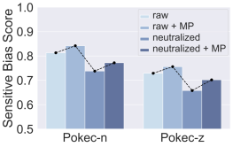
Figure 3: Sensitive biases in four groups of features. The biases are measured by average $\hat{P}_{\theta}(s|x)$, and larger scores indicate more serious sensitive leakage in the representations.

From Figure 3, we can see that message passing enlarges the sensitive biases for both raw and neutralized features, which can validate our theoretical analysis. Also, neutralized features have much less sensitive information leakage, demonstrating the effectiveness of our F3.

Moreover, the estimated feature of heterogeneous neighbors $\operatorname{MLP}_{\phi}(\mathbf{x}_{i})$ can provide additional information when calculating representations, especially for the nodes with few heterogeneous neighbors. Therefore, our method can reach a better performance-fairness trade-off than previous fair GNN methods.

Data-centric v.s. Model-centric Variants.

As pre-processing methods, data-centric variants are task-irrelevant and thus can be employed for various downstream scenarios. For example, we can debias a graph dataset by neutralizing node features in advance, and then graph machine learning algorithms can be trained as usual. Data-centric variants are also more computationally efficient. The model-centric variant is also model-agnostic, and can be combined with any GNN encoders. It allows to further neutralize the internal representations in each GNN layer, and enables additional fairness constraint from an adversarial discriminator. Different parts of the model can learn and improve together, thereby achieving better accuracy and fairness.

Dataset	Bail	Pokec-n	Pokec-z
# Nodes	18,876	66,569	67,797
# Features	18	266	277
# Edges	321,308	729,129	882,765
Node label	Bail decision	Working field	Working field
Sensitive attribute	Race	Region	Region
Avg. degree	34.04	16.53	19.23
Avg. hete-degree	15.79	0.73	0.90
Nodes w/o hete-neighbors	32	46,134	42,783

Table 1: Dataset statistics. “hete-” means “heterogeneous”.

Encoder	Method	Bail				Pokec_n				Pokec_z
		F1↑	ACC↑	DP↓	EO↓	F1↑	ACC↑	DP↓	EO↓	F1↑	ACC↑	DP↓	EO↓
GCN	vanilla	82.04±0.74	87.55±0.54	6.85±0.47	5.26±0.78	67.74±0.41	68.55±0.51	3.75±0.94	2.93±1.15	69.99±0.41	66.78±1.09	3.95±1.03	2.76±0.95
	FairGNN	77.50±1.69	82.94±1.67	6.90±0.17	4.65±0.14	65.62±2.03	67.36±2.06	3.29±2.95	2.46±2.64	70.86±2.36	67.65±1.65	1.87±1.95	1.32±1.42
	EDITS	75.58±3.77	84.49±2.27	6.64±0.39	7.51±1.20	OOM	OOM	OOM	OOM	OOM	OOM	OOM	OOM
	NIFTY	74.76±3.91	82.36±3.91	5.78±1.29	4.72±1.08	64.02±1.26	67.24±0.49	1.22±0.94	2.79±1.24	69.96±0.71	66.74±0.93	6.50±2.16	7.64±1.77
	FairVGNN	79.11±0.33	84.73±0.46	6.53±0.67	4.95±1.22	64.85±1.17	66.10±1.45	1.69±0.79	1.78±0.70	67.31±1.72	61.64±4.72	1.79±1.22	1.25±1.01
	FairSIN-G	79.61±1.29	85.57±1.08	6.57±0.29	5.55±0.84	67.80±0.63	68.22±0.39	2.56±0.60	1.69±1.29	69.68±0.86	65.73±1.76	3.53±1.20	2.42±1.43
	FairSIN-F	82.23±0.63	87.61±0.83	5.54±0.40	3.47±1.03	66.30±0.56	67.96±1.54	1.16±0.90	0.98±0.70	69.74±0.85	66.38±1.39	2.53±0.97	2.03±1.23
	FairSIN w/o Neutral.	81.51±0.33	87.26±0.17	5.93±0.04	4.30±0.20	67.39±0.70	68.35±0.62	2.51±1.99	2.36±1.89	69.18±0.51	65.87±1.34	1.98±1.01	1.87±0.64
	FairSIN w/o Discri.	82.05±0.41	87.40±0.15	5.65±0.40	4.63±0.52	67.94±0.38	68.74±0.33	2.22±1.47	1.67±1.70	69.31±0.63	66.42±1.52	2.73±1.08	2.37±0.69
	FairSIN	82.30±0.63	87.67±0.26	4.56±0.75	2.79±0.89	67.91±0.45	69.34±0.32	0.57±0.19	0.43±0.41	69.24±0.30	67.76±0.71	1.49±0.74	0.59±0.50
GIN	vanilla	77.89±1.09	83.52±0.87	7.55±0.51	6.17±0.69	67.87±0.70	69.25±1.75	3.71±1.20	2.55±1.52	69.49±0.34	65.83±1.31	1.97±1.12	2.17±0.48
	FairGNN	73.67±1.17	77.90±2.21	6.33±1.49	4.74±1.64	64.73±1.86	67.10±3.25	3.82±2.44	3.62±2.78	69.50±2.38	66.49±1.54	3.53±3.90	3.17±3.52
	EDITS	68.07±5.30	73.74±5.12	6.71±2.35	5.98±3.66	OOM	OOM	OOM	OOM	OOM	OOM	OOM	OOM
	NIFTY	70.64±6.73	74.46±9.98	5.57±1.11	3.41±1.43	61.82±3.25	66.37±1.51	3.84±1.05	3.24±1.60	67.61±2.23	65.57±1.34	2.70±1.28	3.23±1.92
	FairVGNN	76.36±2.20	83.86±1.57	5.67±0.76	5.77±0.76	68.01±1.08	68.37±0.97	1.88±0.99	1.24±1.06	68.70±0.89	65.46±1.22	1.45±1.13	1.21±1.06
	FairSIN-G	79.69±0.62	86.10±1.39	6.93±0.16	6.75±0.66	67.16±1.03	67.73±1.67	1.98±1.54	1.50±1.15	68.84±1.96	65.09±2.69	1.55±1.23	1.74±0.80
	FairSIN-F	80.37±0.84	86.48±0.75	5.95±1.85	5.97±2.07	68.36±0.55	68.92±1.08	1.51±1.11	0.82±0.79	68.96±1.08	65.97±0.82	1.45±1.15	1.14±0.73
	FairSIN w/o Neutral.	79.33±0.64	85.27±0.70	7.21±0.39	6.75±0.55	68.30±1.12	68.92±1.13	2.81±1.91	2.12±1.30	69.38±1.28	65.04±1.56	2.19±1.96	1.23±0.92
	FairSIN w/o Discri.	80.14±1.06	86.44±0.80	4.38±1.48	4.23±1.88	67.32±0.36	70.04±0.80	2.44±1.50	1.63±1.24	69.21±0.25	65.58±0.71	1.40±0.67	1.12±0.24
	FairSIN	80.44±1.14	86.52±0.48	4.35±0.71	4.17±0.96	68.43±0.64	69.58±0.57	1.11±0.31	0.97±0.59	69.06±0.54	66.74±1.56	0.64±0.47	1.01±0.64
SAGE	vanilla	83.03±0.42	88.13±1.12	1.13±0.48	2.61±1.16	67.15±0.88	69.03±0.77	3.09±1.29	2.21±1.60	70.24±0.46	66.55±0.69	4.71±1.05	2.72±0.85
	FairGNN	82.55±0.98	87.68±0.73	1.94±0.82	1.72±0.70	65.75±1.89	67.03±2.61	2.97±1.28	2.06±3.02	69.49±2.15	67.68±1.49	2.86±1.39	2.30±1.33
	EDITS	77.83±3.79	84.42±2.87	3.74±3.54	4.46±3.50	OOM	OOM	OOM	OOM	OOM	OOM	OOM	OOM
	NIFTY	77.81±6.03	84.11±5.49	5.74±0.38	4.07±1.28	61.70±1.47	68.48±1.11	3.84±1.05	3.90±2.18	66.86±2.51	66.68±1.45	6.75±1.84	8.15±0.97
	FairVGNN	83.58±1.88	88.41±1.29	1.14±0.67	1.69±1.13	67.40±1.20	68.50±0.71	1.12±0.98	1.13±1.02	69.91±0.95	66.39±1.95	4.15±1.30	2.31±1.57
	FairSIN-G	83.96±1.78	88.79±1.08	3.97±0.92	1.70±0.66	68.08±1.10	69.11±0.62	2.00±1.13	1.66±0.70	71.05±0.73	66.19±1.49	4.96±0.25	2.90±1.21
	FairSIN-F	83.82±0.26	88.51±0.16	0.67±0.33	1.85±0.50	67.21±0.84	69.28±0.98	1.80±0.46	1.62±0.84	70.25±0.40	66.99±1.06	3.25±1.00	1.89±0.79
	FairSIN w/o Neutral.	82.95±0.46	87.70±0.28	0.64±0.40	2.21±0.22	67.38±0.81	68.77±0.62	2.35±0.99	1.71±0.99	69.87±1.70	67.39±1.05	2.92±1.69	1.79±1.16
	FairSIN w/o Discri.	83.49±0.34	88.46±0.19	0.82±0.51	2.12±0.55	67.14±1.09	69.65±0.32	1.91±0.82	1.09±1.12	70.10±0.93	66.78±0.83	3.92±1.02	1.62±0.68
	FairSIN	83.97±0.43	88.74±0.42	0.58±0.60	1.49±0.34	68.38±0.83	69.12±1.16	1.04±0.83	1.04±0.42	70.70±0.99	67.95±0.79	1.74±0.73	0.68±0.65

Table 2: Comparison among SOTA methods and different variants of FairSIN. (Bold: the best; underline: the runner-up.)

4 Experiments

In this section, we thoroughly evaluate and analyze the effectiveness of our proposed method. Specifically, we follow the experimental setup of (Wang et al. 2022c; Dong et al. 2022a), and consider both fairness and accuracy metrics across multiple datasets. Our experiments are conducted to answer the following research questions (RQs):

RQ1: How effective is our proposed method compared with SOTA graph fairness methods? RQ2: How does each module of our proposed method contribute to the final performance? RQ3: How does the hyper-parameter $\delta$ influence the performance? RQ4: How does the time cost of our method compared with other baselines?

4.1 Experimental Settings

Datasets.

Following the approaches proposed in (Wang et al. 2022c; Dong et al. 2022a), we evaluate FairSIN and baseline methods on five real-world benchmark datasets: German (Asuncion and Newman 2007), Credit (Yeh and Lien 2009), Bail (Jordan and Freiburger 2015) and Pokec-n/Pokec-z (Takac and Zabovsky 2012). These datasets have been extensively used in previous studies on graph fairness learning, and cover a diverse range of domains, including finance, criminal justice and social network. We provide the dataset statistics in Table 1.

GNN Backbones.

In our experiments, we employ three commonly used graph neural networks (GNNs) as the backbone of our encoder: GCN (Kipf and Welling 2017), GIN (Xu et al. 2019), and GraphSAGE (Hamilton, Ying, and Leskovec 2017). These encoders have been widely adopted by the research community and have demonstrated strong performance on various graph-related tasks.

Baselines.

We compare our methods with the following state-of-the-art fair node representation learning methods. FairGNN (Dai and Wang 2021): a debiasing method based on adversarial training. EDITS (Dong et al. 2022a): an augmentation-based method minimizing discrimination between different sensitive groups by pruning the graph topology and node features. NIFTY (Agarwal, Lakkaraju, and Zitnik 2021): a method that integrates feature perturbation and edge dropping to enforce counterfactual fairness constraints by maximizing the similarity between augmented and counterfactual graphs. FairVGNN (Wang et al. 2022c): a framework preventing sensitive attribute leakage by masking sensitive-correlated channels and adaptively clamping weights. All baselines are implemented based on the given three GNN backbones.

Evaluation Metrics.

To assess the performance of downstream classification task, we employ F1 score and accuracy as the metrics. To evaluate group fairness, we adopt Demographic (Statistical) Parity (DP) (Dwork et al. 2012) and Equal Opportunity (EO)  (Hardt, Price, and Srebro 2016) as previous studies (Agarwal, Lakkaraju, and Zitnik 2021; Dai and Wang 2021; Wang et al. 2022c; Dong et al. 2022a). Note that a model with lower DP and EO implies better fairness.

Implementation Details.

For our proposed method, we leverage a 3-layer MLP to predict the features or representations of heterogeneous neighbors. Specifically, we adopt an Adam optimizer for MLP with weight decay in {0.001, 0.0001, 0} and tune the learning rate in {0.1,0.01,0.001}. The dropout rate is in {0.2, 0.5, 0.8}. In addition, we tune the coefficient hyper-parameter $\delta$ in our proposed method over the range of [0,10]. For GNN encoders, we use the same settings as (Wang et al. 2022c). We report mean and standard deviation over five runs with different random seeds. All our experiments are run on a single GPU device of GeForce GTX 3090 with 22 GB memory.

4.2 Main Results (RQ1)

Effectiveness of Model-centric Variant FairSIN.

Here we present the results of FairSIN to demonstrate that our neutralization-based strategy can achieve a better trade-off than SOTA methods. As shown in Table 2, FairSIN has both the best overall classification performance and group fairness under different GNN encoders. In terms of fairness, FairSIN respectively reduces DP and EO by 63.29% and 33.82%, compared with the best performed baseline. Additionally, since the F3 can introduce extra neighborhood information for each node, in many cases FairSIN can even outperform the vanilla encoder in accuracy metrics. Compared to Bail, Pokec-n/Pokec-z have very few heterogeneous neighbors. Hence, the improvement achieved by FairSIN is more pronounced on the Pokec dataset, aligning with our motivation and model design.

Effectiveness of Data-centric Variants FairSIN-G and FairSIN-F.

Here we can compare our proposed data-centric variants with a previous pre-processing method EDITS (Dong et al. 2022a) as well as the vanilla encoder. From Table 2, we can see that both FairSIN-G and FairSIN-F maintain the accuracy and improve the fairness on average, which demonstrates our idea of sensitive information neutralization. Also, FairSIN-G only amplifies the weights of existing heterogeneous neighbors, which limits its capacity to furnish as extensive information as FairSIN-F. Consequently, in comparison, the predictive performance of FairSIN-G falls short when contrasted with FairSIN-F. It is worth noting that as a pre-processing method, FairSIN-F is only slightly worse than the model-centric variant FairSIN, and outperforms previous SOTA methods. Therefore, FairSIN-F offers a cost-effective, model-agnostic and task-irrelevant solution for fair node representation learning.

4.3 Ablation Study (RQ2)

To fully evaluate the effects of each component used in our proposed FairSIN, we consider two ablated models: FairSIN w/o Discri. denotes the version of FairSIN without the discriminator, and FairSIN w/o Neutral. denotes the version of FairSIN where $\delta=0$. Experimental results are listed in Table 2. The relative improvement brought by F3 on Bail is not as significant as that on Pokec, since nodes in Bail dataset have almost equal number of homogeneous and heterogeneous neighbors. Broadly speaking, both F3 and the discriminator yield beneficial outcomes. However, when the discriminator is employed in isolation rather than as a constraint to guide the learning of F3, it often leads to a decrease in predictive precision. It is worth noting that the neutralization of F3 alone, i.e., FairSIN w/o Discri., can already achieve a favorable trade-off between fairness and accuracy metrics, and is the most important design in our model.

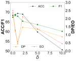
(a)

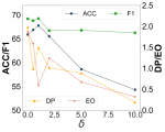
(b)

Figure 4: Classification performance and group fairness under different values of hyper-parameter $\delta$.

4.4 Hyper-parameter Analysis (RQ3)

The value of $\delta$ is crucial to FairSIN as it can control the amount of introduced heterogeneous information. It is important to choose a proper value of $\delta$, as setting it too large may lead to sensitive information leakage in an opposite direction. We investigate the effect of hyper-parameter $\delta$ over {0, 0.5, 1, 2, 5, 10} with GCN encoder, and present the results in Figure 4. For Pokec-n and Pokec-z datasets, we can observe an optimal value $\delta=1$, where a favorable trade-off between predictive performance and fairness can be reached. The distribution of heterogeneous neighbors is too sparse on Pokec dataset as we can see in Table 1, thus fairness are improving when $\delta$ increases to 10. In terms of predictive performance on Pokec-n, both accuracy and F1 score exhibit a decline as $\delta$ increases. As for Pokec-z, a similar trend is observed with the exception that the F1 score maintains a relatively stable level. In general, excessively large values of $\delta$ contribute to a decrease in predictive performance for both datasets. These observations align with our idea of neutralization. Hyper-parameter experiment on German, Credit and Bail can be found in Appendix.

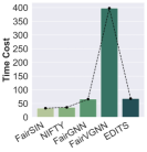
(a)

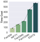
(b)

Figure 5: Training time cost on Bail and Credit with GCN backbone (in seconds).

4.5 Efficiency Analysis (RQ4)

As shown in Figure 5, we compare the training time cost of our FairSIN with the baselines on Bail and Credit datasets. We can find that FairSIN has the lowest time cost among all methods. Thus our method is both efficient and effective, enabling potential applications in various scenarios. FairVGNN (Wang et al. 2022c) incurs such high time cost attributed to its large number of parameters and the process of adverserial training. Also, EDITS (Dong et al. 2022a) needs to model node similarities between all node pairs for edge addition, and thus incurs a high time complexity.

5 Conclusion

In this paper, we propose the neutralization-based strategy FairSIN for learning fair GNNs, where extra F3 are added to node features or representations before message passing. By emphasizing the features of each node’s heterogeneous neighbors, F3 can simultaneously neutralize the sensitive bias in node representations and provide extra non-sensitive feature information. We further present three implementation variants from both data-centric and model-centric perspectives. Extensive experimental results demonstrate the motivation and effectiveness of our proposed method.

We hope this work can provide a new paradigm to the area of fair GNNs, and thus keep our implementation as simple as possible. For future work, we can explore alternatives with wider receptive field and more complex architecture to replace MLPs for F3 estimator. Besides, current F3 are irrelevant to downstream tasks, and it is also possible to build task-specific ones. In addition, when we need to handle multiple sensitive groups at the same time, we can extend F3 to neutralize a joint distribution of sensitive attributes.

References

- Agarwal, Lakkaraju, and Zitnik (2021) Agarwal, C.; Lakkaraju, H.; and Zitnik, M. 2021. Towards a unified framework for fair and stable graph representation learning. In Uncertainty in Artificial Intelligence, 2114–2124. PMLR.
- Asuncion and Newman (2007) Asuncion, A.; and Newman, D. 2007. UCI machine learning repository.
- Bongini, Bianchini, and Scarselli (2021) Bongini, P.; Bianchini, M.; and Scarselli, F. 2021. Molecular generative graph neural networks for drug discovery. Neurocomputing, 450: 242–252.
- Bose and Hamilton (2019) Bose, A.; and Hamilton, W. 2019. Compositional fairness constraints for graph embeddings. In International Conference on Machine Learning, 715–724. PMLR.
- Chen et al. (2021) Chen, H.; Wang, L.; Lin, Y.; Yeh, C.-C. M.; Wang, F.; and Yang, H. 2021. Structured graph convolutional networks with stochastic masks for recommender systems. In Proceedings of the 44th International ACM SIGIR Conference on Research and Development in Information Retrieval, 614–623.
- Chouldechova and Roth (2018) Chouldechova, A.; and Roth, A. 2018. The frontiers of fairness in machine learning. arXiv preprint arXiv:1810.08810.
- Dai and Wang (2021) Dai, E.; and Wang, S. 2021. Say no to the discrimination: Learning fair graph neural networks with limited sensitive attribute information. In Proceedings of the 14th ACM International Conference on Web Search and Data Mining, 680–688.
- Dong et al. (2021) Dong, Y.; Kang, J.; Tong, H.; and Li, J. 2021. Individual fairness for graph neural networks: A ranking based approach. In Proceedings of the 27th ACM SIGKDD Conference on Knowledge Discovery & Data Mining, 300–310.
- Dong et al. (2022a) Dong, Y.; Liu, N.; Jalaian, B.; and Li, J. 2022a. Edits: Modeling and mitigating data bias for graph neural networks. In Proceedings of the ACM Web Conference 2022, 1259–1269.
- Dong et al. (2023) Dong, Y.; Ma, J.; Wang, S.; Chen, C.; and Li, J. 2023. Fairness in graph mining: A survey. IEEE Transactions on Knowledge and Data Engineering.
- Dong et al. (2022b) Dong, Y.; Wang, S.; Wang, Y.; Derr, T.; and Li, J. 2022b. On structural explanation of bias in graph neural networks. In Proceedings of the 28th ACM SIGKDD Conference on Knowledge Discovery and Data Mining, 316–326.
- Dwork et al. (2012) Dwork, C.; Hardt, M.; Pitassi, T.; Reingold, O.; and Zemel, R. 2012. Fairness through awareness. In Proceedings of the 3rd innovations in theoretical computer science conference, 214–226.
- Edwards and Storkey (2015) Edwards, H.; and Storkey, A. 2015. Censoring representations with an adversary. arXiv preprint arXiv:1511.05897.
- Field et al. (2021) Field, A.; Blodgett, S. L.; Waseem, Z.; and Tsvetkov, Y. 2021. A survey of race, racism, and anti-racism in NLP. Annual Meeting of the Association for Computational Linguistics.
- Fisher et al. (2020) Fisher, J.; Mittal, A.; Palfrey, D.; and Christodoulopoulos, C. 2020. Debiasing knowledge graph embeddings. In Proceedings of the 2020 Conference on Empirical Methods in Natural Language Processing (EMNLP), 7332–7345.
- Hamilton, Ying, and Leskovec (2017) Hamilton, W.; Ying, Z.; and Leskovec, J. 2017. Inductive representation learning on large graphs. Advances in neural information processing systems, 30.
- Hardt, Price, and Srebro (2016) Hardt, M.; Price, E.; and Srebro, N. 2016. Equality of opportunity in supervised learning. Advances in neural information processing systems, 29.
- Holstein et al. (2019) Holstein, K.; Wortman Vaughan, J.; Daumé III, H.; Dudik, M.; and Wallach, H. 2019. Improving fairness in machine learning systems: What do industry practitioners need? In Proceedings of the 2019 CHI conference on human factors in computing systems, 1–16.
- Jiang et al. (2022) Jiang, Z.; Han, X.; Fan, C.; Liu, Z.; Zou, N.; Mostafavi, A.; and Hu, X. 2022. Fmp: Toward fair graph message passing against topology bias. arXiv preprint arXiv:2202.04187.
- Jordan and Freiburger (2015) Jordan, K. L.; and Freiburger, T. L. 2015. The effect of race/ethnicity on sentencing: Examining sentence type, jail length, and prison length. Journal of Ethnicity in Criminal Justice, 13(3): 179–196.
- Kang et al. (2022) Kang, J.; Zhu, Y.; Xia, Y.; Luo, J.; and Tong, H. 2022. Rawlsgcn: Towards rawlsian difference principle on graph convolutional network. In Proceedings of the ACM Web Conference 2022, 1214–1225.
- Kipf and Welling (2017) Kipf, T. N.; and Welling, M. 2017. Semi-supervised classification with graph convolutional networks. International Conference on Learning Representations.
- Kose and Shen (2022) Kose, O. D.; and Shen, Y. 2022. Fair node representation learning via adaptive data augmentation. arXiv preprint arXiv:2201.08549.
- Kusner et al. (2017) Kusner, M. J.; Loftus, J.; Russell, C.; and Silva, R. 2017. Counterfactual fairness. Advances in neural information processing systems, 30.
- La Fond and Neville (2010) La Fond, T.; and Neville, J. 2010. Randomization tests for distinguishing social influence and homophily effects. In Proceedings of the 19th international conference on World wide web, 601–610.
- Laclau et al. (2021) Laclau, C.; Redko, I.; Choudhary, M.; and Largeron, C. 2021. All of the fairness for edge prediction with optimal transport. In International Conference on Artificial Intelligence and Statistics, 1774–1782. PMLR.
- Lambrecht and Tucker (2019) Lambrecht, A.; and Tucker, C. 2019. Algorithmic bias? An empirical study of apparent gender-based discrimination in the display of STEM career ads. Management science, 65(7): 2966–2981.
- Li et al. (2021) Li, P.; Wang, Y.; Zhao, H.; Hong, P.; and Liu, H. 2021. On dyadic fairness: Exploring and mitigating bias in graph connections. In International Conference on Learning Representations.
- Li et al. (2020) Li, Z.; Shen, X.; Jiao, Y.; Pan, X.; Zou, P.; Meng, X.; Yao, C.; and Bu, J. 2020. Hierarchical bipartite graph neural networks: Towards large-scale e-commerce applications. In 2020 IEEE 36th International Conference on Data Engineering (ICDE), 1677–1688. IEEE.
- Liao et al. (2019) Liao, J.; Huang, C.; Kairouz, P.; and Sankar, L. 2019. Learning generative adversarial representations (GAP) under fairness and censoring constraints. arXiv preprint arXiv:1910.00411, 1.
- Ling et al. (2023) Ling, H.; Jiang, Z.; Luo, Y.; Ji, S.; and Zou, N. 2023. Learning fair graph representations via automated data augmentations. In The Eleventh International Conference on Learning Representations.
- McPherson, Smith-Lovin, and Cook (2001) McPherson, M.; Smith-Lovin, L.; and Cook, J. M. 2001. Birds of a feather: Homophily in social networks. Annual review of sociology, 27(1): 415–444.
- Mehrabi et al. (2021) Mehrabi, N.; Morstatter, F.; Saxena, N.; Lerman, K.; and Galstyan, A. 2021. A survey on bias and fairness in machine learning. ACM Computing Surveys (CSUR), 54(6): 1–35.
- Niu et al. (2020) Niu, X.; Li, B.; Li, C.; Xiao, R.; Sun, H.; Deng, H.; and Chen, Z. 2020. A dual heterogeneous graph attention network to improve long-tail performance for shop search in e-commerce. In Proceedings of the 26th ACM SIGKDD International Conference on Knowledge Discovery & Data Mining, 3405–3415.
- Rahman et al. (2019) Rahman, T.; Surma, B.; Backes, M.; and Zhang, Y. 2019. Fairwalk: Towards fair graph embedding.
- Shervashidze et al. (2011) Shervashidze, N.; Schweitzer, P.; Van Leeuwen, E. J.; Mehlhorn, K.; and Borgwardt, K. M. 2011. Weisfeiler-lehman graph kernels. Journal of Machine Learning Research, 12(9).
- Shumovskaia et al. (2021) Shumovskaia, V.; Fedyanin, K.; Sukharev, I.; Berestnev, D.; and Panov, M. 2021. Linking bank clients using graph neural networks powered by rich transactional data. International Journal of Data Science and Analytics, 12: 135–145.
- Spinelli et al. (2021) Spinelli, I.; Scardapane, S.; Hussain, A.; and Uncini, A. 2021. Fairdrop: Biased edge dropout for enhancing fairness in graph representation learning. IEEE Transactions on Artificial Intelligence, 3(3): 344–354.
- Sun et al. (2019) Sun, T.; Gaut, A.; Tang, S.; Huang, Y.; ElSherief, M.; Zhao, J.; Mirza, D.; Belding, E.; Chang, K.-W.; and Wang, W. Y. 2019. Mitigating gender bias in natural language processing: Literature review. Annual Meeting of the Association for Computational Linguistics.
- Takac and Zabovsky (2012) Takac, L.; and Zabovsky, M. 2012. Data analysis in public social networks. In International scientific conference and international workshop present day trends of innovations, volume 1.
- Veličković et al. (2018) Veličković, P.; Cucurull, G.; Casanova, A.; Romero, A.; Lio, P.; and Bengio, Y. 2018. Graph attention networks. International Conference on Learning Representations.
- Wang et al. (2022a) Wang, N.; Lin, L.; Li, J.; and Wang, H. 2022a. Unbiased graph embedding with biased graph observations. In Proceedings of the ACM Web Conference 2022, 1423–1433.
- Wang et al. (2022b) Wang, R.; Wang, X.; Shi, C.; and Song, L. 2022b. Uncovering the Structural Fairness in Graph Contrastive Learning. Advances in neural information processing systems.
- Wang et al. (2022c) Wang, Y.; Zhao, Y.; Dong, Y.; Chen, H.; Li, J.; and Derr, T. 2022c. Improving fairness in graph neural networks via mitigating sensitive attribute leakage. In KDD, 1938–1948.
- Xiong et al. (2021) Xiong, J.; Xiong, Z.; Chen, K.; Jiang, H.; and Zheng, M. 2021. Graph neural networks for automated de novo drug design. Drug Discovery Today, 26(6): 1382–1393.
- Xu et al. (2019) Xu, K.; Hu, W.; Leskovec, J.; and Jegelka, S. 2019. How powerful are graph neural networks? International Conference on Learning Representations.
- Yeh and Lien (2009) Yeh, I.-C.; and Lien, C.-h. 2009. The comparisons of data mining techniques for the predictive accuracy of probability of default of credit card clients. Expert systems with applications, 36(2): 2473–2480.