SC-Diff: 3D Shape Completion with Latent Diffusion Models

Abstract

This paper introduces a 3D shape completion approach using a 3D latent diffusion model optimized for completing shapes, represented as Truncated Signed Distance Functions (TSDFs), from partial 3D scans. Our method combines image-based conditioning through cross-attention and spatial conditioning through the integration of 3D features from captured partial scans. This dual guidance enables high-fidelity, realistic shape completions at superior resolutions. At the core of our approach is the compression of 3D data into a low-dimensional latent space using an auto-encoder inspired by 2D latent diffusion models. This compression facilitates the processing of higher-resolution shapes and allows us to apply our model across multiple object classes, a significant improvement over other existing diffusion-based shape completion methods, which often require a separate diffusion model for each class. We validated our approach against two common benchmarks in the field of shape completion, demonstrating competitive performance in terms of accuracy and realism and performing on par with state-of-the-art methods despite operating at a higher resolution with a single model for all object classes. We present a comprehensive evaluation of our model, showcasing its efficacy in handling diverse shape completion challenges, even on unseen object classes. The code will be released upon acceptance.

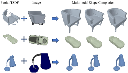
Figure 1: Our method produces realistic and accurate object shape completions from realistic partial scans with a higher degree of detail than state-of-the-art methods, including 3D-EPN [12] and AutoSDF [22]. Image input is optional in our work.

1 Introduction

The evolution of digital technologies has revolutionized the role of 3D content, particularly in areas like augmented/virtual reality, gaming, robot navigation, and industrial design. These domains rely heavily on the creation and manipulation of 3D models, a process that remains technically challenging and labor-intensive, often requiring specialized skills and tools.

A significant development in this landscape in recent years has been the widespread of commodity RGB-D sensors (e.g., Intel RealSense, Microsoft Kinect, iPhone, etc.). These sensors have enabled remarkable progress in 3D reconstruction and understanding, facilitating the generation of detailed 3D models from the real world. The ability to use these sensors for high-quality scanning has far-reaching implications, from enhancing virtual reality experiences to improving the accuracy of robot navigation and streamlining design processes in various industries.

However, despite advancements in reconstruction quality [1, 25], the scans obtained from RGB-D sensors are often partial or fragmented, leaving gaps in reconstructing complete 3D models. This fundamental challenge arises due to environmental obstacles and the restricted sensor reach, both of which impede the attainment of complete scanning. Addressing this challenge is vital for fully utilizing 3D scanning technologies and maximizing the potential of 3D content in the aforementioned fields.

Recently, a variety of learning-based methods for 3D shape completion have emerged, utilizing techniques such as fully convolutional networks [13] and transformer based architectures [38]. These approaches typically focus on establishing a direct mapping function between partial scans and their complete counterparts. However, they can sometimes encounter limitations, such as overfitting and the potential introduction of artifacts. In contrast, probabilistic methods approach shape completion as a conditional generation task, offering the flexibility to produce multiple plausible outcomes. This category includes innovative solutions like variational auto-encoders [22], adversarial training [41], and diffusion models [6, 23, 8, 7], which collectively represent a significant advancement in generating diverse and realistic shape completions in scenarios with inherent ambiguity.

Diffusion models have achieved significant success in various image generation tasks, especially in text-conditional and image-conditional generation [15, 31]. Advances such as ControlNet [42] have introduced spatially consistent conditioning mechanisms, enhancing control over the spatial composition of generated images. This makes diffusion models highly promising for the conditional completion of 3D shapes. Latest methods like SDFusion [6] and DiffRF [6] conceptualize shape completion as filling artificially generated missing cubic regions, but this does not fully address the challenges of realistic sensor-captured 3D shapes, which often have varying levels of incompleteness and noise [6, 23].

In this paper, we present an approach for 3D shape completion from partial scans, aiming to produce realistic, high-fidelity, complete shapes. We complete a Truncated Signed Distance Function (TSDF) based 3D shape representation with a latent diffusion model, integrating image-based and spatially consistent conditioning inspired by ControlNet [42]. Our approach utilizes an auto-encoder architecture trained on both 3D and 2D objectives [36, 14] to compress the input TSDF into a lower dimensional latent space, enabling the processing of higher resolution shapes efficiently in the diffusion model (moving from $32^{3}$ to $64^{3}$ TSDF voxel grids). When compared to a non-latent approach, our latent-diffusion model uses $30.72\%$ less GPU Memory. This addresses the common challenge of high computational demands that limit existing 3D generative models to lower resolutions [8, 6].

The key contributions of this work are:

• Compression of 3D shapes into a latent space, enabling the processing of voxel grids of higher resolutions and the learning of diffusion-based shape completion for multiple classes with a single model.

• Involving both 3D supervision and volume rendering-enabled 2D supervision for the learning of the Vector Quantised Variational AutoEncoder (VQ-VAE) resulting in a compact representation of the input TSDFs.

• Incorporating two independent and complementary conditioning mechanisms: image-based conditioning with cross-attention and spatial conditioning, integrating 3D features from partial scans inspired by DiffComplete  [8].

2 Related Work

Traditional approaches to 3D shape completion primarily focus on repairing minor imperfections and geometrical gaps, employing strategies like Laplacian hole filling [17] and Poisson surface reconstruction [4]. While effective for filling small gaps in the 3D shapes, these methods are of limited use in scenarios with a larger scale of gaps in the input scans. However, the advent of extensive 3D datasets has led to the development of learning-based approaches. While retrieval-based methods [3, 40, 2] extract the most fitting shapes from a database to complete the incomplete input, learning-based fitting methods [39, 12, 10, 14, 37] that aim to minimize the disparity between network-predicted shapes and actual ground truth have become more prevalent. Examples of such methods are 3D-EPN [12] and Scan2Mesh [11] which have employed 3D encoder-decoder architectures for predicting complete shapes from partial volumetric data. More recently, PatchComplete [29] introduces a novel design by learning multi-resolution patch priors, enhancing the completion of shapes, particularly for previously unseen categories. While these models can provide high-accuracy completions, their deterministic nature may lead to overfitting. Furthermore, they often lack the ability to generate finer details in shapes.

Generative methods, including Generative Adversarial Networks (GANs) [41] and AutoEncoders [22], have recently been introduced to the field. These methods excel in generating a diverse range of plausible shapes from partial inputs. However, this often comes at the cost of accuracy, especially when a precise ground truth is available. Diffusion models have emerged as a popular family of generative models, renowned for their impressive quality, diversity, and expressiveness in tasks such as image synthesis [31], image editing [20], and text-to-image synthesis [28]. While extensively researched for 2D data, their application to 3D data has only been explored very recently, using different 3D representations such as point-clouds [19, 44] neural radiance fields [21], or signed distance functions [7, 18]. SDFusion [6], specifically, introduces a latent diffusion model for shape generation aimed at mitigating the computational challenges associated with 3D representations, and conditions it on various modalities like images, text, and shapes. However, SDFusion merely regards completion as extending a partial but complete shape by filling artificially cropped out 3D boxes. In contrast, our approach does not make any assumption on the partial shape as real-world scans are characterized by noise and varying degrees of incompleteness. Another approach, DiffComplete [8], offers a more realistic shape completion method but directly works on the 3D space and is therefore restricted to lower-resolution voxel grids of size $32^{3}$. As opposed to DiffComplete, our approach can achieve much higher resolution by encoding the 3D space to compact latent codes. Furthermore, most previous methods [29, 23, 21] work on the assumption that the object class is known prior to the completion, which makes them hard to deploy in real-world applications. In contrast, our model is class-agnostic, and outputs high-detailed, realistic completions, even for unseen classes.

3 Methodology

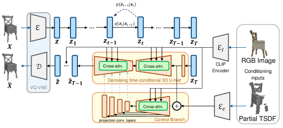
Figure 2: We train a Vector Quantized Variational Autoencoder (VQ-VAE) to encode complete TSDF voxel grids $\mathbf{X}$ into a compact latent variable $\mathbf{z}$. Then, we use this learned latent space to train our conditional shape completion diffusion model. First, we corrupt the clean latent code z through a forward diffusion process $q(\mathbf{z}_{t}|\mathbf{z}_{-1})$ by gradually adding Gaussian noise until reaching the normally distributed variable $\mathbf{z}_{T}$. Our diffusion model is then trained to learn the reverse diffusion process $p_{\theta}(\mathbf{z}_{t-1}|\mathbf{z}_{t})$ conditioned on a partial TSDF scan c of the shape by aggregating features from a control branch and/or a partial RGB image $\mathbf{I}$ of the shape by applying cross-attention on CLIP Features of the given images. This process allows us to recover the latent code $\mathbf{\hat{z}}$, and finally, using the VQ-VAE’s decoder, the completed shape $\mathbf{\hat{X}}$.

We approach 3D shape completion as a generative task based on a diffusion probabilistic model, aiming to produce a complete shape $\hat{\mathbf{X}}$ from a given partial scan represented by an RGB Image $\mathbf{I}$ and a partial 3D TSDF $\mathbf{c}$. While diffusion models have proven highly effective in generating high-resolution images, their direct application to high-resolution 3D shapes is hindered by the substantial demands on computation and memory. Consequently, 3D diffusion-based approaches are often confined to low-resolution voxel grids, typically around $32^{3}$  [6, 22]. To address this limitation, we first compress the 3D shape into a compact latent space using a Vector Quantized Variational Autoencoder (VQ-VAE), as detailed in Sec. 3.1. This VQ-VAE is trained with supervision from both 3D TSDF, and 2D depth and normal renderings from a raycasting-based volume rendering approach [14]. This compression strategy allows us to implement our diffusion model in a lower-dimensional space, a process referred to as Latent Diffusion (Sec. 3.2). Our model includes two distinct conditioning mechanisms (Sec. 3.3) in the generative process: the first leverages RGB Image $\mathbf{I}$’s CLIP features  [27] via cross attention, and the second uses spatially localized conditions [42, 8] derived from the 3D partial scans $\mathbf{c}$. An overview of our approach is provided in Fig. 2.

3.1 3D Shape Compression

Processing high-resolution 3D shapes poses significant computational demands. To accommodate this in the diffusion model, we compress the TSDF-based 3D shape representation $\mathbf{X}\in\mathbb{R}^{S\times S\times S}$ into a lower-dimensional latent space $\mathbf{z}\in\mathbb{R}^{D\times S_{l}\times S_{l}\times S_{l}}$, where $D$ and $S_{l}$ represent the feature size and the downsampled spatial size. As shown by the seminal work on 2D image generation using Latent Diffusion Models [31], the compression preprocessing before generation allows our diffusion model to focus more effectively on the generative aspect of the shape completion process.

3.1.1 Vector Quantized Variational Autoencoder

We employ a 3D Variant of the Vector Quantized Variational Autoencoder (VQ-VAE)  [36, 30] for condensing the compressed latent spaces of various shapes. The architecture of VQ-VAE consists of an encoder $\mathcal{E}$, a decoder $\mathcal{D}$, and a codebook $\bm{\mathcal{Z}}\in\mathbb{R}^{K_{\mathcal{Z}}\times D}$, with $K_{\mathcal{Z}}$ and $D$ representing the codebook’s length and the dimensionality of each latent vector, respectively.

For a given TSDF volume $\mathbf{X}$, encoding into a latent representation is done as $\mathbf{z}=\mathcal{E}(\mathbf{X})$. The decoder then reconstructs $\mathbf{X^{\prime}}=\mathcal{D}(Q(\mathbf{z}))$ from $\mathbf{z}$, where $Q(\cdot)$ represents the quantization step, mapping each of the latent vectors $\mathbf{z}_{i}$ in $\mathbf{z}$ to the nearest codebook vector $\bm{\mathcal{Z}}_{j}$ using $Q(\mathbf{z}_{i})=\bm{\mathcal{Z}}_{j}$, where $j=\arg\min_{k\in[1,K_{z}]}||\mathbf{z}_{i}-\bm{\mathcal{Z}}_{k}||_{2}$. Here, $\bm{\mathcal{Z}}_{k}$ corresponds to $k$th elements of $\bm{\mathcal{Z}}$.

We pre-train our VQ-VAE loss with the following 3D losses:

• Reconstruction Loss minimizes the difference between the input and reconstructed TSDF voxel grid: $\mathcal{L}_{R}=||\mathbf{X}-\mathbf{X^{\prime}}||_{1}$

• Commitment Loss encourages the encoder output to stay close to the selected codebook vector, using the stop-gradient operator $\cancel{S}(\cdot)$: $\mathcal{L}_{C}=\beta||\mathbf{z}-\cancel{S}(Q(\mathbf{z}))||_{2}^{2}$

• Codebook Loss ensures the chosen codebook vector aligns with the encoder output:

  $\mathcal{L}_{CB}=(1-\beta)||\cancel{S}(\mathbf{z})-Q(\mathbf{z})||_{2}^{2}$

Alongside 3D losses, our methodology incorporates 2D supervision from rendering the reconstructed TSDF grids $\mathbf{X^{\prime}}$, inspired by SPSG [14]. We render both depth ($\mathbf{D_{v}^{\prime}}$) and normal images ($\mathbf{N_{v}^{\prime}}$) from $\mathbf{X^{\prime}}$ at each camera view $v$ in a differentiable manner via raycasting-based volume rendering.

The 2D supervision losses employed for VQ-VAE training include:

• 2D Reconstruction Loss: An $l_{1}$ loss guiding depth and normal reconstruction:

  $$\mathcal{L}_{R_{2D}}=||\mathbf{D_{v}}-\mathbf{D_{v}^{\prime}}||_{1}+||\mathbf{N_{v}}-\mathbf{N_{v}^{\prime}}||_{1}$$ (1)

  where $\mathbf{D_{v}}$ and $\mathbf{N_{v}}$ correspond to the ground-truth depth and normal values, and $\mathbf{D_{v}^{\prime}}$ and $\mathbf{N_{v}^{\prime}}$ are the rendered depth and normal images.

• 2D Adversarial Loss: A patch-based adversarial loss on normals $\mathbf{N_{v}^{\prime}}$ for realistic geometry reconstruction:

  $$L_{A_{2D}}= \mathbb{E}_{\mathbf{N_{v}}}(\log\mathrm{Disc}(\mathbf{N_{v}}))+$$

  $$\mathbb{E}_{\mathbf{N_{v}^{\prime}}}(\log(1-\mathrm{Disc}(\mathbf{N_{v}^{\prime}}))),$$ (2)

  where $\mathrm{Disc}(\cdot)$ denotes the CNN based discriminator network.

The final VQ-VAE objective combines both 3D and 2D losses:

$$\mathcal{L}_{VQVAE}=\mathcal{L}_{R}+\beta\mathcal{L}_{C}+(1-\beta)\mathcal{L}_{CB}+\gamma_{R}\mathcal{L}_{R_{2D}}+\gamma_{A}L_{A_{2D}},$$ (3)

where $\lambda$, $\gamma_{R}$, and $\gamma_{A}$ are hyperparameters balancing the different losses. Our experiments (Sec. 4.2) demonstrate that this 2D supervision enhances reconstruction quality, especially in capturing finer geometric details, leading to an improved encoding $\mathbf{z}$ of the input TSDFs.

3.2 Latent Diffusion Model for 3D Shapes

Utilizing our pre-trained VQ-VAE, we remap TSDFs into a low-dimensional latent space for efficiently training our diffusion model. Fundamentally, Diffusion models  [15, 31] learn a data distribution $p(\mathbf{z})$ by denoising a variable $\mathbf{\mathbf{z}_{T}}$, starting from a normal distribution. Our goal is to model this reverse diffusion process with a Deep Neural Network with parameters $\mathbf{\theta}$.

3.2.1 Forward Diffusion Process

The forward diffusion process is a fixed Markov Chain, adding Gaussian noise to a latent sample $\mathbf{z}$ over time steps $t\in{1,...,T}$, following a variance schedule $\beta_{1},\beta_{2},...\beta_{T}$ [15] (see Eq. 4, Fig. 2).

$$q(\mathbf{z}_{1:T}|\mathbf{z}_{0}):=\prod_{t=1}^{T}q(\mathbf{z}_{t}|\mathbf{z}_{t-1})\text{,}$$

$$q(\mathbf{z}_{t}|\mathbf{z}_{t-1}):=\mathcal{N}(\mathbf{z}_{t};\sqrt{1-\beta_{t}}\mathbf{z}_{t-1},\beta_{t}\mathbf{I}).$$ (4)

3.2.2 Reverse Diffusion Process

The reverse process is defined as a learned Markov Chain with learned Gaussian transitions starting at $p(\mathbf{z}_{T})=\mathcal{N}(\mathbf{z}_{T};\mathbf{0},\mathbf{I})$ as follows [15]:

$$p_{\theta}(\mathbf{z}_{0:T}):=p(\mathbf{z}_{T})\prod_{t=1}^{T}p_{\theta}(\mathbf{z}_{t-1}|\mathbf{z}_{t},\mathbf{c},\mathbf{I})\text{,}$$

$$p_{\theta}(\mathbf{z}_{t-1}|\mathbf{z}_{t}):=\mathcal{N}(\mathbf{z}_{t-1};\bm{\mu}_{\theta}(\mathbf{z}_{t},t,\mathbf{c},\mathbf{I}),\bm{\Sigma}_{\theta}(\mathbf{z}_{t},t,\mathbf{c},\mathbf{I}))$$ (5)

Where $\mathbf{c}$ and $\mathbf{I}$ are the partial TSDF and RGB image respectively, and $\bm{\mu}_{\theta}$ and $\bm{\Sigma}_{\theta}$ are the mean and covariance predicted by our network in latent space. Learning the reverse diffusion process involves estimating these mean and covariance. However, it has been shown experimentally that setting $\bm{\Sigma}_{\theta}(\mathbf{z}_{t},t,\mathbf{c},\mathbf{I})=\sigma_{t}^{2}\mathbf{I}$ with $\sigma_{t}^{2}=\tilde{\beta}_{t}=\frac{1-\bar{\alpha}_{t-1}}{1-\bar{\alpha}_{t}}\beta_{t}$ with $\alpha_{t}:=1-\beta_{t}$ and $\bar{\alpha}_{t}:=\prod_{s=1}^{t}\alpha_{s}$ provides good results, while removing the need to learn the covariance.

We use the reparametrization and objective proposed by  [15] (see Eq. 6) and focus on predicting the noise $\bm{\epsilon}_{\theta}(\mathbf{z}_{t},t)$ added during the forward process.

$$L_{simple}(\theta):=\mathbb{E}_{t,\mathbf{z},\bm{\epsilon}}\left[\|\bm{\epsilon}-\bm{\epsilon}_{\theta}(\mathbf{z}_{t},t,\mathbf{c},\mathbf{I})\|_{2}^{2}\right].$$ (6)

At training time, we take a complete TSDF voxel grid $\mathbf{X}$  and compute a latent code $\mathbf{z}_{0}$ using our VQ-VAE’s encoder $\mathcal{E}$, then we sample a noised latent code $\mathbf{z}_{t}$ at time $t$. The denoising diffusion model predicts the noise $\bm{\epsilon}_{\theta}(\mathbf{z}_{t},t)$ and is trained with the objective shown in Eq. 6.

In contrast, at inference time, we sample $\mathbf{\hat{z}}$ by gradually denoising a noise variable $\textbf{z}_{T}$ sampled from the standard normal distribution $\mathcal{N}(\mathbf{z}_{T};\mathbf{0},\mathbf{I})$ and then use our pretrained decoder $\mathcal{D}$ and codebook $\mathcal{Z}$ to map the denoised code $\mathbf{\hat{z}}$ back to a predicted complete TSDF voxel grid $\mathbf{\hat{X}}$.

Our denoising diffusion model $\bm{\epsilon}_{\theta}(\mathbf{z}_{t},t)$ is implemented as a time-conditional 3D U-Net  [15, 31].

3.3 Conditioning mechanisms

We propose the use of two conditioning mechanisms, as depicted in Fig. 2: cross-attention on CLIP features [27] from an object image and spatially consistent feature aggregation from a partial scan’s TSDF voxel grid.

3.3.1 Conditioning 3D shape generation on RGB Images

Diffusion models are capable of modeling conditional distributions of the form $p(\mathbf{z}|\mathbf{y})$, which allows us to implement a conditional denoising autoencoder $\epsilon_{\theta}(z_{t},t,y)$ where $y$ is a conditioning input.

Inspired by latent diffusion models [31], we extend the U-Net backbone with a cross-attention mechanism. This allows learning the distribution of latent codes $p(\mathbf{z}|\mathcal{E}_{I}(\mathbf{I}))$ conditioned on pre-trained CLIP encoder features of an RGB image of the 3D object rendered from the pose where the partial scan was taken.

The CLIP encoder $\mathcal{E}_{I}$ projects the RGB Image $\mathbf{I}\in\mathbb{R}^{3\times 256\times 256}$ to an intermediate representation $\mathcal{E}_{I}(\mathbf{I})\in\mathbb{R}^{M\times d_{\mathcal{E}_{I}}}$ where $d_{\mathcal{E}_{I}}=768$ is the dimension of the CLIP features and $M=50$ corresponds to the flattened spatial dimension of CLIP’s encoding. This representation is then mapped to the flattened intermediate layers of the time-conditional UNet via cross-attention layers.

3.3.2 Conditioning 3D shape generation on Partial Scans

Simultaneously, to enhance control over the spatial composition and address limitations of image-only conditioning, we introduce a second mechanism inspired by ControlNet and DiffComplete [42, 8].

First, the corrupted ground truth latent code $\mathbf{z}_{t}$ and partial shape $\mathbf{c}$ are encoded into multi-resolution feature maps of the same size $\mathcal{E}_{\epsilon}(\mathbf{z}_{t})$ and $\mathcal{E}_{c}(\mathbf{c})$ respectively. While the diffusion model forwards $\mathcal{E}_{\epsilon}(\mathbf{z}_{t})$, the control branch propagates the fused features $\mathbf{f}=\mathcal{E}_{\epsilon}(\mathbf{z}_{t})+\mathcal{E}_{c}(\mathbf{c})$ into deeper layers. The control branch is connected to the diffusion model with projection 1x1 convolutional layers such that the feature maps have consistent sizes and can be aggregated. The features that enter the i-th decoder block of the diffusion model are denoted as:

$$d^{(i)}=[\mathcal{D}_{z}^{(i-1)}(\mathbf{z}_{t}),F_{z}^{(i)}(\mathbf{z}_{t})+\phi^{(i)}(F_{c}^{(i)}(\mathbf{f}))]$$ (7)

Where $\phi^{(i)}$ is the 1x1 convolutional projection layer, $F_{z}^{(i)}(\mathbf{z}_{t})$ are the encoder features of the diffusion model’s i-th encoder block that are passed through residual connections to the decoder block $\mathcal{D}_{z}^{(i-1)}$. $F_{c}^{(i)}(\mathbf{f})$ corresponds to the features of the control branch’s i-th encoder block, and $[\cdot,\cdot]$ is the concatenation operation.

Combining the presented conditioning approaches allows the model to leverage global shape cues from images and detailed 3D information from partial scans, facilitating realistic and high-fidelity shape completion.

Table 1: Quantitative comparison on the 3D-EPN benchmark [12]. Our class-specific model consistently outperforms all state-of-the-art methods in reconstruction accuracy, while it still achieves competitive results when generalizing over all classes.

$l1$-err $\downarrow$	3D-EPN	AutoSDF	PatchComplete	DiffComplete	Ours	Ours	Ours
	[12]	[22]	[29]	[8]
resolution	$32^{3}$	$32^{3}$	$32^{3}$	$32^{3}$	$32^{3}$	$64^{3}$	$64^{3}$
class-specific	x	x	x	✓	x	x	✓
Chair	0.418	0.201	0.134	0.070	0.082	0.086	0.078
Table	0.377	0.258	0.095	0.073	0.074	0.074	0.075
Sofa	0.392	0.226	0.084	0.061	0.070	0.075	0.055
Lamp	0.388	0.275	0.087	0.059	0.047	0.048	0.037
Plane	0.421	0.184	0.061	0.015	0.015	0.017	0.014
Car	0.259	0.187	0.053	0.025	0.032	0.041	0.033
Cabinet	0.381	0.248	0.134	0.086	0.095	0.091	0.065
Watercraft	0.356	0.157	0.058	0.031	0.028	0.028	0.024
Avg.	0.374	0.217	0.088	0.053	0.055	0.058	0.047

4 Experiments

We evaluate our method in the task of shape completion on two large-scale shape completion benchmarks. The 3D-EPN [12] dataset contains 25,590 object instances of eight classes from ShapeNet [5]. For each instance, several partial scans of varying completeness are provided as $32^{3}$ TSDF grids, while complete shapes are represented as $32^{3}$ or $64^{3}$ truncated unsigned distance functions. The Patchcomplete [29] benchmark emphasizes completing objects from unseen categories. It contains 5000 partial/complete pairs from the synthetic Shapenet [5] and 11,000 partial/complete pairs taken from objects in the scenes of the real-world ScanNet dataset [9].

We first train a VQ-VAE for 150k steps. Next, we train our conditional shape completion network (diffusion model + control branch) using the same data split for other 200k steps, while the CLIP encoder remains frozen with pre-trained weights. In both cases we use Adam optimizer [43] with a learning rate of $1\times 10^{-4}$ and $2.5\times 10^{-5}$, respectively. We set our batch size to $8$ and trained both VQ-VAE and our shape completion network on a single Nvidia A40 GPU with 48GB of VRAM. While the VQ-VAE can be trained in 48 hours, training the diffusion model takes about 120 hours. On the other hand, at inference we use the formulation of DDIM [34], needing only 100 denoising steps which take about 15 seconds per sample.

4.1 Quantitative Evaluation

As commonly used in the field, we evaluate the $l_{1}$ error across all voxels for known object classes as well as the chamfer distance (CD), and the Intersection over Union (IoU) between predicted and ground truth shapes for unknown classes.

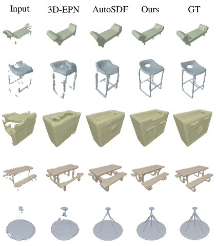
Figure 3: Shape completion results on the test set of the 3D-EPN [12] benchmark. DiffComplete [8] results are not shown due to the lack of open-source code and weights.

4.1.1 3D-EPN Benchmark - Known Object Classes:

Our method demonstrates competitive performance when directly compared to the state-of-the-art techniques by training class-specific models, outperforming them by a $\downarrow 12\%$ reduction in l1 (see Tab. 1). It is noteworthy that our class-agnostic model still has similar performance to the class-specific state-of-the-art model Diffcomplete [8], and outperforms the other compared class-agnostic models, which showcases its great generalization capabilities. Unlike the compared techniques, our method additionally uses the RGB image from the partial scans. Furthermore, it is important to highlight that the compared approaches are designed to operate on a $32^{3}$ resolution, whereas our model is capable of processing $64^{3}$ TSDF voxel grids. As shown qualitatively in Fig. 1, our diffusion-based approach excels in predicting fine-detailed shapes from the partial input scans.

Table 2: Quantitative comparison for shape completion results for unknown categories on the Patchcomplete benchmark [29] at a $32^{3}$ resolution. Top: results for synthetic shapes from the Shapenet dataset [5]. Bottom: results for real objects from the Scannet dataset [9]

CD$\downarrow$/IoU$\uparrow$	3D-EPN	Auto-SDF	PatchComplete	DiffComplete	Ours
	[12]	[22]	[29]	[8]
Bag	5.01 / 73.8	5.81 / 56.3	3.94 / 77.6	3.86 / 78.30	3.79 / 78.26
Lamp	8.07 / 47.2	6.57 / 39.1	4.68 / 56.4	4.80 / 57.90	4.74 / 59.95
Bathtub	4.21 / 57.9	5.17 / 41.0	3.78 / 66.30	3.52 / 68.90	3.67 / 65.88
Bed	5.84 / 58.4	6.01 / 44.6	4.49 / 66.8	4.16 / 67.10	4.40 / 67.05
Basket	7.90 / 54.0	6.70 / 39.8	5.15 / 61.0	4.94 / 65.50	4.89 / 68.45
Printer	5.15 /73.6	5.82 / 49.9	4.63 / 77.6	4.40 / 76.80	4.36 / 76.77
Laptop	3.90 / 62.0	4.81 / 51.1	3.77 / 63.8	3.52 / 67.40	3.41 / 68.35
Bench	4.54 / 48.3	4.31 / 39.5	3.70 / 53.9	3.56 / 58.20	3.39 / 61.13
Avg.	5.58 / 59.4	5.86 / 45.2	4.27 / 65.4	4.10 / 67.50	4.08 / 68.17

CD$\downarrow$/IoU$\uparrow$	3D-EPN	Auto-SDF	PatchComplete	DiffComplete	Ours
	[12]	[22]	[29]	[8]
Bag	8.83 / 53.7	9.30 / 48.7	8.23 / 58.3	7.05 / 48.5	7.41 / 50.02
Lamp	14.3 / 20.7	11.2 / 24.4	9.42 / 28.4	6.84 / 30.5	6.39 / 33.17
Bathtub	7.56 / 41.0	7.84 / 36.6	6.77 / 48.0	8.22 / 48.50	8.09 / 48.44
Bed	7.76 / 47.8	7.91 / 38.0	7.24 / 48.4	7.20 / 46.6	6.91 / 48.63
Basket	7.74 / 36.5	7.54 / 36.1	6.60 / 45.5	7.42 / 59.2	6.38 / 62.15
Printer	8.36 / 63.0	9.66 / 49.9	6.84 / 70.5	6.36 / 74.5	7.10 / 69.06
Avg.	9.09 / 44.0	8.90 / 38.9	7.52 / 49.5	7.18 / 51.3	7.04 / 51.91

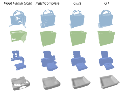
Figure 4: Qualitative Results on the Patchcomplete [29] benchmark for unseen categories.

4.1.2 Patchcomplete Benchmark - Unseen Object Classes:

For object categories not observed during training our method outperforms competitors in several specific categories such as bag, basket, lamp, and bench, and it also shows a marginal overall improvement for both synthetic and real-world data (see Tab. 2). Such outcomes can be attributed to the efficacy of our dual conditioning mechanisms, which effectively guide the latent diffusion model’s generative process, thereby ensuring the completion of shapes with a high grade of fidelity. Fig. 4 shows some of the predictions performed by our method on this benchmark, showcasing its superior ability to complete shapes from unseen categories with inputs of various levels of completeness.

It is noteworthy to highlight the probabilistic nature of our method, which inherently allows for multiple potential shape completions from the same input, as depicted in Fig. 5. This characteristic is particularly advantageous in the context of shape completion, a problem intrinsically under-constrained and characterized by a multitude of feasible solutions. Consequently, it is beneficial for a method to not only generate realistic, high-fidelity outcomes but also to offer a diversity of results that encapsulate the range of possible solutions. Our approach successfully achieves this balance, showcasing its versatility in handling the complexity of the shape completion task.

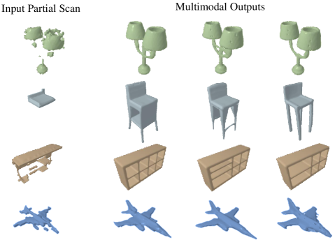
Figure 5: Our approach produces diverse but realistic and detailed multimodal shape completions for the same input partial scans.

4.1.3 Comparison to SDFusion [6]:

Metric	SDFusion	Ours
l1-error $\downarrow$	0.086	0.068
CD $\downarrow$	0.058	0.025
IoU $\uparrow$	0.38	0.55

Table 3: Comparison between SDFusion[6] and our method.

Even though our purpose was to perform shape completion from partial scans, we also compared the performance of our model with a state of the art method for 3D Latent Diffusion: SDFusion [6]. For this, we adopted their formulation of shape completion where the partial TSDFs are obtained by masking out big regions of the ground truth shapes, and finetuned our model for $50k$ further steps.

As shown in Tab. 3. Our method significantly outperforms SDFusion [6] in l1-error, chamfer distance, and IoU. Similarly, Fig. 6 shows how our method produces both more plausible and more diverse shapes.

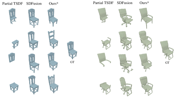
Figure 6: Shape completion comparison with SDFusion[6]. Our method produces more plausible and diverse results.

4.2 Ablation Studies

4.2.1 Influence of 2D Loss on VQ-VAE Performance:

Table 4: Effect of 2D losses on VQ-VAE’s reconstructions.

2D Loss weight $(\gamma)$	$l1$-err $\downarrow$	IoU $\uparrow$
0.0	6.49$e^{-3}$	88.48
0.2	4.06$e^{-3}$	91.54
0.4	2.99$e^{-3}$	93.15
0.6	3.48$e^{-3}$	92.97

We extend the original VQ-VAE [36] by incorporating supplementary 2D losses that operate on 2D renderings of the reconstructed TSDFs. Tab. 4 demonstrates the beneficial impact of these added 2D objectives on the autoencoder’s shape reconstructions, evidencing a substantial enhancement in reconstruction quality, with a $\downarrow 54\%$ reduction in $l1$ error and a $\uparrow 6\%$ increase in IoU.

4.2.2 Effects of different conditioning Types:

Table 5: Impact of the different conditioning mechanisms evaluated on the 3D-EPN dataset.

Image-based	Partial TSDF	Avg. $l1$-err $\downarrow$
✓		0.341
	✓	0.072
✓	✓	0.058

Tab. 5 shows the impact of implementing our conditioning mechanisms by evaluating performance on the 3DEPN benchmark under three distinct scenarios: image-based conditioning alone, partial shape-based conditioning alone, and the concurrent application of both conditioning strategies. While relying solely on image-based conditioning yields suboptimal performance attributable to the inherent uncertainties in the image-to-shape reconstruction task, the synergy of image-based and partial shape conditionings results in a notable $15\%$ reduction in $l1$-error respect to partial shape conditioning only. This demonstrates that while each conditioning mechanism contributes uniquely, their combination harnesses their respective strengths to significantly enhance the shape completion process, allowing for a competitive performance even when we train a single model to predict complete shapes for multiple object categories.

5 Conclusion

In this work, we have developed a latent diffusion-based approach for 3D shape completion, integrating a latent diffusion model with a VQ-VAE. When enhanced with 2D losses, this combination effectively compresses TSDF voxel grids into a compact latent space. In that way, our approach surpasses typical resolution limits seen in current diffusion-based methods, achieving $64^{3}$ resolution and generalizing across multiple object classes, in contrast to class-specific models like DiffComplete [8]. By incorporating a spatially consistent conditioning mechanism we can generate diverse and realistic shapes from partial scans, providing a significant advantage over other state-of-the-art methods such as SDFusion [6] and DiffRF [23], which tackle the shape completion task by filling out artificially cropped out boxes.

Despite these advancements, challenges remain, particularly in processing complex scenes at higher resolutions. Future work will focus on addressing these limitations. Integrating preprocessing steps for accurate object bounding box and pose determination, as seen in existing methods  [24, 16, 26], could expand the method’s usability in practical scenarios beyond the positioning of single objects in a canonical space. Additionally, while diffusion models offer high-quality sample generation, their relatively slow sampling speed is a notable drawback. Emerging research in areas like non-Markovian diffusion processes  [34], progressive distillation  [33], and consistency models  [35] present potential pathways to improve efficiency in conditional generation across various data modalities, including 3D shapes.

Appendix 0.A Detailed Network Architecture

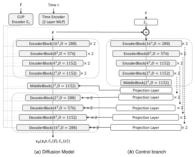
Figure 7: Our diffusion model’s architecture (a) is connected with a Control branch (b). Both encoder and decoder contain eight blocks with two spatial transformers at resolutions $2^{3}$ and $4^{3}$. Each transformer contains several attention and self-attention mechanisms.

Our diffusion model is fundamentally a 3D version of a ControlNet [42]. Similar to DiffComplete [8] and SDFusion [6], our neural network is implemented using a 3D U-Net [32] with an encoder, a middle block, and a decoder, which is connected to the encoder through skip connections. Both the encoder and decoder contain ResNetBlocks. In the case of the encoder, these are accompanied by downsampling blocks, while in the decoder, they are accompanied by up-sampling convolution layers. The encoder, decoder, and middle block include two spatial transformers each. Images are encoded using CLIP encoder [27], and diffusion timesteps are encoded with a 2-layer MLP using positional encoding. Similarly, the control branch shares the same architecture as the diffusion model up to the middle block. Then, it uses 3D convolutional projection layers to feed partial shape’s $\mathbf{c}$ intermediate representation into the diffusion model spatially consistently. (See Fig. 7).

Appendix 0.B Hyperparameter Values

The Tab. 6 shows the hyperparameters chosen in our experiments.

Table 6: Values for most important hyperparameters.

Name	Symbol	Value
TSDF Truncation threshold	$thresh$	$3.0$
Resolution of the TSDF voxel grid	$S$	$64$
Resolution of the latent space	$S_{l}$	$16$
Feature size of the VQ-VAE’s latent space	$D$	$3$
Codebook Size	$K_{\mathcal{Z}}$	$16,384$
3D Commitment Loss weight for VQ-VAE	$\beta$	$0.5$
2D Reconstruction Loss weight for VQ-VAE	$\gamma_{R}$	$0.4$
2D Adversarial Loss weight for VQ-VAE	$\gamma_{A}$	$0.4$
Diffusion timesteps at training	$T$	$1000$
Diffusion timesteps at inference (DDIM [34])	$T_{inf}$	$100$
Diffusion variance start value	$\beta_{1}$	$8.5e^{-4}$
Diffusion variance end value	$\beta_{T}$	$0.012$
Attention resolutions	$A_{res}$	$[2,4]$
CLIP Features size	$D_{CLIP}$	$768$
Batch Size	$bs$	$8$
Learning Rate VQ-VAE	$lr_{vqvae}$	$1e^{-4}$
Learning Rate Diffusion Model	$lr_{diff}$	$2.5e^{-5}$

Appendix 0.C Forward and backward diffusion processes

As shown in Fig. 8, the forward diffusion process is a fixed Markov chain that gradually corrupts a latent code $\mathbf{z}_{0}$ by adding Gaussian noise with a given variance schedule. Transitions are defined by $q(\mathbf{z}_{t}|\mathbf{z}_{t-1})$ in Eq. 4. We train a diffusion model to learn the reverse denoising process with transitions $p_{\theta}(\mathbf{z}_{t-1}|\mathbf{z}_{t})$ as shown in Eq. 5

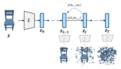
Figure 8: Forward Diffusion Process. After passing them through our pretrained decoder $\mathcal{D}$, we illustrate how the shapes recovered from the corrupted latent codes look.

Appendix 0.D Effect of 2D Loss on VQ-VAE Performance

Fig. 9 shows a qualitative illustration of the efficacy of integrating a 2D objective to create high-fidelity reconstructions. As illustrated, the 2D losses help improve the reconstruction of fine-grained details of the object, such as the individual elements of a chair’s backrest.

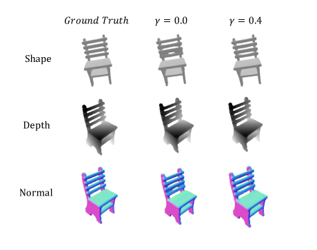
Figure 9: The introduction of 2D losses improves the VQ-VAE’s reconstruction, thus improving the learning of the latent space.

Appendix 0.E Effect of different conditioning types

Fig. 10 illustrates a visual comparison of the proposed conditioning mechanisms: Image Only, Partial TSDF Only, and Multimodal Conditioning. We conducted five predictions on each input using the specified conditioning mechanism and selected the prediction with the lowest L1 error. While image-only conditioning leads to severe over-smoothing of the reconstructed object, only conditioning on the partial TSDF misses many details. The results underscore the enhanced effectiveness of utilizing both conditioning mechanisms in tandem over image-only conditioning, which proves insufficient to obtain high-quality results.

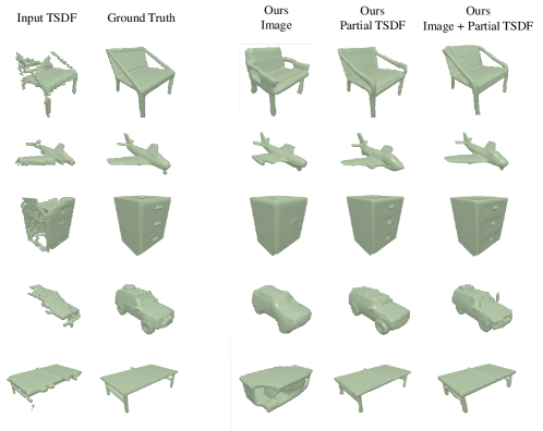
Figure 10: Comparison of different types of conditioning.

Appendix 0.F More multimodal results

Fig. 11 shows more multimodal predictions our model performs.

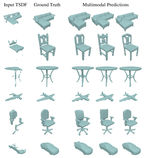
Figure 11: Further multimodal predictions performed by our model

Appendix 0.G Failure Cases

To evaluate the instances where our model does not perform as expected, we carry out five predictions for a given input and select the one with the highest L1 error. This approach enables us to obtain predictions like those shown in Fig. 12. Owing to the intrinsic ambiguity of the shape completion task and the significant incompleteness of some partial scans, the predicted shapes might not only appear unrealistic but also be completed as entirely different objects. This issue partly stems from the fact that our model is class-agnostic.

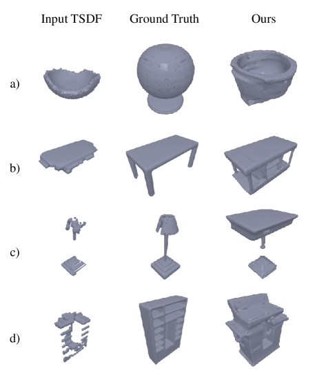
Figure 12: Examples of instances where our model failed to accurately predict high-fidelity and realistic shapes. a) The model predicts the shape as a type of container, even though the ground-truth shape is a lamp. b) Our latent diffusion model unnecessarily predicts a more complex shape than the ground truth. c) and d) Given the high level of incompleteness of the input, the model completes the shape as a completely different class; for instance, it predicts a table and sofa instead of the actual ground truth, which are a lamp and cabinet

References

- [1] Azinović, D., Martin-Brualla, R., Goldman, D.B., Nießner, M., Thies, J.: Neural rgb-d surface reconstruction. In: Proceedings of the IEEE/CVF Conference on Computer Vision and Pattern Recognition. pp. 6290–6301 (2022)
- [2] Beyer, T., Dai, A.: Weakly-supervised end-to-end cad retrieval to scan objects. arXiv preprint arXiv:2203.12873 (2022)
- [3] Bosche, F., Haas, C.T.: Automated retrieval of 3d cad model objects in construction range images. Automation in Construction 17(4), 499–512 (2008)
- [4] Centin, M., Pezzotti, N., Signoroni, A.: Poisson-driven seamless completion of triangular meshes. Computer Aided Geometric Design 35, 42–55 (2015)
- [5] Chang, A.X., Funkhouser, T., Guibas, L., Hanrahan, P., Huang, Q., Li, Z., Savarese, S., Savva, M., Song, S., Su, H., et al.: Shapenet: An information-rich 3d model repository. arXiv preprint arXiv:1512.03012 (2015)
- [6] Cheng, Y.C., Lee, H.Y., Tulyakov, S., Schwing, A.G., Gui, L.Y.: Sdfusion: Multimodal 3d shape completion, reconstruction, and generation. In: Proceedings of the IEEE/CVF Conference on Computer Vision and Pattern Recognition. pp. 4456–4465 (2023)
- [7] Chou, G., Bahat, Y., Heide, F.: Diffusion-sdf: Conditional generative modeling of signed distance functions. In: Proceedings of the IEEE/CVF International Conference on Computer Vision. pp. 2262–2272 (2023)
- [8] Chu, R., Xie, E., Mo, S., Li, Z., Nießner, M., Fu, C.W., Jia, J.: Diffcomplete: Diffusion-based generative 3d shape completion. In: Thirty-seventh Conference on Neural Information Processing Systems (2023)
- [9] Dai, A., Chang, A.X., Savva, M., Halber, M., Funkhouser, T., Nießner, M.: Scannet: Richly-annotated 3d reconstructions of indoor scenes. In: Proceedings of the IEEE conference on computer vision and pattern recognition. pp. 5828–5839 (2017)
- [10] Dai, A., Diller, C., Nießner, M.: Sg-nn: Sparse generative neural networks for self-supervised scene completion of rgb-d scans. In: Proceedings of the IEEE/CVF Conference on Computer Vision and Pattern Recognition. pp. 849–858 (2020)
- [11] Dai, A., Nießner, M.: Scan2mesh: From unstructured range scans to 3d meshes. In: Proceedings of the IEEE/CVF Conference on Computer Vision and Pattern Recognition. pp. 5574–5583 (2019)
- [12] Dai, A., Ruizhongtai Qi, C., Nießner, M.: Shape completion using 3d-encoder-predictor cnns and shape synthesis. In: Proceedings of the IEEE conference on computer vision and pattern recognition. pp. 5868–5877 (2017)
- [13] Dai, A., Ruizhongtai Qi, C., Nießner, M.: Shape completion using 3d-encoder-predictor cnns and shape synthesis. In: Proceedings of the IEEE conference on computer vision and pattern recognition. pp. 5868–5877 (2017)
- [14] Dai, A., Siddiqui, Y., Thies, J., Valentin, J., Nießner, M.: Spsg: Self-supervised photometric scene generation from rgb-d scans. In: Proceedings of the IEEE/CVF Conference on Computer Vision and Pattern Recognition. pp. 1747–1756 (2021)
- [15] Ho, J., Jain, A., Abbeel, P.: Denoising diffusion probabilistic models. Advances in neural information processing systems 33, 6840–6851 (2020)
- [16] Huang, S., Qi, S., Xiao, Y., Zhu, Y., Wu, Y.N., Zhu, S.C.: Cooperative holistic scene understanding: Unifying 3d object, layout, and camera pose estimation. Advances in Neural Information Processing Systems 31 (2018)
- [17] Li, H., Luo, L., Vlasic, D., Peers, P., Popović, J., Pauly, M., Rusinkiewicz, S.: Temporally coherent completion of dynamic shapes. ACM Transactions on Graphics (TOG) 31(1), 1–11 (2012)
- [18] Li, Y., Dou, Y., Chen, X., Ni, B., Sun, Y., Liu, Y., Wang, F.: Generalized deep 3d shape prior via part-discretized diffusion process. In: Proceedings of the IEEE/CVF Conference on Computer Vision and Pattern Recognition. pp. 16784–16794 (2023)
- [19] Lyu, Z., Kong, Z., Xu, X., Pan, L., Lin, D.: A conditional point diffusion-refinement paradigm for 3d point cloud completion. arXiv preprint arXiv:2112.03530 (2021)
- [20] Meng, C., He, Y., Song, Y., Song, J., Wu, J., Zhu, J.Y., Ermon, S.: Sdedit: Guided image synthesis and editing with stochastic differential equations. arXiv preprint arXiv:2108.01073 (2021)
- [21] Metzer, G., Richardson, E., Patashnik, O., Giryes, R., Cohen-Or, D.: Latent-nerf for shape-guided generation of 3d shapes and textures. Proceedings of the IEEE/CVF Conference on Computer Vision and Pattern Recognition (2022)
- [22] Mittal, P., Cheng, Y.C., Singh, M., Tulsiani, S.: Autosdf: Shape priors for 3d completion, reconstruction and generation. In: Proceedings of the IEEE/CVF Conference on Computer Vision and Pattern Recognition. pp. 306–315 (2022)
- [23] Müller, N., Siddiqui, Y., Porzi, L., Bulo, S.R., Kontschieder, P., Nießner, M.: Diffrf: Rendering-guided 3d radiance field diffusion. In: Proceedings of the IEEE/CVF Conference on Computer Vision and Pattern Recognition. pp. 4328–4338 (2023)
- [24] Nie, Y., Han, X., Guo, S., Zheng, Y., Chang, J., Zhang, J.J.: Total3dunderstanding: Joint layout, object pose and mesh reconstruction for indoor scenes from a single image. In: Proceedings of the IEEE/CVF Conference on Computer Vision and Pattern Recognition. pp. 55–64 (2020)
- [25] Park, J.J., Florence, P., Straub, J., Newcombe, R., Lovegrove, S.: Deepsdf: Learning continuous signed distance functions for shape representation. In: Proceedings of the IEEE/CVF conference on computer vision and pattern recognition. pp. 165–174 (2019)
- [26] Pintore, G., Agus, M., Gobbetti, E.: Atlantanet: inferring the 3d indoor layout from a single 360 ∘ image beyond the manhattan world assumption. In: European Conference on Computer Vision. pp. 432–448. Springer (2020)
- [27] Radford, A., Kim, J.W., Hallacy, C., Ramesh, A., Goh, G., Agarwal, S., Sastry, G., Askell, A., Mishkin, P., Clark, J., et al.: Learning transferable visual models from natural language supervision. In: International conference on machine learning. pp. 8748–8763. PMLR (2021)
- [28] Ramesh, A., Dhariwal, P., Nichol, A., Chu, C., Chen, M.: Hierarchical text-conditional image generation with clip latents. arXiv preprint arXiv:2204.06125 1(2), 3 (2022)
- [29] Rao, Y., Nie, Y., Dai, A.: Patchcomplete: Learning multi-resolution patch priors for 3d shape completion on unseen categories. Advances in Neural Information Processing Systems 35, 34436–34450 (2022)
- [30] Razavi, A., Van den Oord, A., Vinyals, O.: Generating diverse high-fidelity images with vq-vae-2. Advances in neural information processing systems 32 (2019)
- [31] Rombach, R., Blattmann, A., Lorenz, D., Esser, P., Ommer, B.: High-resolution image synthesis with latent diffusion models. In: Proceedings of the IEEE/CVF conference on computer vision and pattern recognition. pp. 10684–10695 (2022)
- [32] Ronneberger, O., Fischer, P., Brox, T.: U-net: Convolutional networks for biomedical image segmentation. In: Medical Image Computing and Computer-Assisted Intervention–MICCAI 2015: 18th International Conference, Munich, Germany, October 5-9, 2015, Proceedings, Part III 18. pp. 234–241. Springer (2015)
- [33] Salimans, T., Ho, J.: Progressive distillation for fast sampling of diffusion models. arXiv preprint arXiv:2202.00512 (2022)
- [34] Song, J., Meng, C., Ermon, S.: Denoising diffusion implicit models. arXiv preprint arXiv:2010.02502 (2020)
- [35] Song, Y., Dhariwal, P., Chen, M., Sutskever, I.: Consistency models. arXiv preprint arXiv:2303.01469 (2023)
- [36] Van Den Oord, A., Vinyals, O., et al.: Neural discrete representation learning. Advances in neural information processing systems 30 (2017)
- [37] Xu, B., Davison, A.J., Leutenegger, S.: Learning to complete object shapes for object-level mapping in dynamic scenes. In: 2022 IEEE/RSJ International Conference on Intelligent Robots and Systems (IROS). pp. 2257–2264. IEEE (2022)
- [38] Yan, X., Lin, L., Mitra, N.J., Lischinski, D., Cohen-Or, D., Huang, H.: Shapeformer: Transformer-based shape completion via sparse representation. In: Proceedings of the IEEE/CVF Conference on Computer Vision and Pattern Recognition. pp. 6239–6249 (2022)
- [39] Yuan, W., Khot, T., Held, D., Mertz, C., Hebert, M.: Pcn: Point completion network. In: 2018 international conference on 3D vision (3DV). pp. 728–737. IEEE (2018)
- [40] Zhang, C., Zhou, G., Yang, H., Xiao, Z., Yang, X.: View-based 3-d cad model retrieval with deep residual networks. IEEE Transactions on Industrial Informatics 16(4), 2335–2345 (2019)
- [41] Zhang, J., Chen, X., Cai, Z., Pan, L., Zhao, H., Yi, S., Yeo, C.K., Dai, B., Loy, C.C.: Unsupervised 3d shape completion through gan inversion. In: Proceedings of the IEEE/CVF Conference on Computer Vision and Pattern Recognition. pp. 1768–1777 (2021)
- [42] Zhang, L., Rao, A., Agrawala, M.: Adding conditional control to text-to-image diffusion models. In: Proceedings of the IEEE/CVF International Conference on Computer Vision. pp. 3836–3847 (2023)
- [43] Zhang, Z.: Improved adam optimizer for deep neural networks. In: 2018 IEEE/ACM 26th international symposium on quality of service (IWQoS). pp. 1–2. Ieee (2018)
- [44] Zhou, L., Du, Y., Wu, J.: 3d shape generation and completion through point-voxel diffusion. In: Proceedings of the IEEE/CVF International Conference on Computer Vision. pp. 5826–5835 (2021)
Supplementary Material