Inflation Target at Risk: A Time-varying Parameter Distributional Regression

Abstract

Macro variables frequently display time-varying distributions, driven by the dynamic and evolving characteristics of economic, social, and environmental factors that consistently reshape the fundamental patterns and relationships governing these variables. To better understand the distributional dynamics beyond the central tendency, this paper introduces a novel semi-parametric approach for constructing time-varying conditional distributions, relying on the recent advances in distributional regression. We present an efficient precision-based Markov Chain Monte Carlo algorithm that simultaneously estimates all model parameters while explicitly enforcing the monotonicity condition on the conditional distribution function. Our model is applied to construct the forecasting distribution of inflation for the U.S., conditional on a set of macroeconomic and financial indicators. The risks of future inflation deviating excessively high or low from the desired range are carefully evaluated. Moreover, we provide a thorough discussion about the interplay between inflation and unemployment rates during the Global Financial Crisis, COVID, and the third quarter of 2023.

Keywords: Time-varying Parameter Model, Distributional Regression, Bayesian Analysis, Inflation Risks
JEL Codes: C11, C14, E63

1 Introduction

The incorporation of time-varying parameter (TVP) models holds a fundamental and crucial role in macroeconomic analysis, as evidenced by seminal works such as those by Stock and Watson (1996), Cogley and Sargent (2005), and Primiceri (2005). By allowing model parameters to evolve over time, these models can capture the changing dynamics and structural shifts inherent in macroeconomic variables. The literature has extensively utilized TVP regression models to uncover reliable predictors of inflation, with notable contributions from Koop and Korobilis (2012), Belmonte et al. (2014), and Chan (2017). For a deeper exploration of TVP models and their application in macroeconomic analysis, see Koop and Korobilis (2013), Clark and Ravazzolo (2015), Chan (2023), among many others. Despite their strengths, a limitation of these models lies in their primary focus on the conditional mean. This could potentially miss the full spectrum of data distribution, such as tail behaviors or distributional spread that could provide critical insights into economic phenomena.

In this paper, we develop a time-varying parameter distributional regression (TVP-DR) model for analyzing the evolving conditional distribution of a time series based on the current state of the economy, that elicits the time-varying features of the entire conditional distribution. Distributional regression (DR) was initially introduced by Williams and Grizzle (1972) to analyze ordered categorical outcomes using multiple binary regressions. It was later extended by Foresi and Peracchi (1995) to characterize any univariate conditional distribution. Chernozhukov et al. (2013) introduced DR for estimating counterfactual distributions and provided valid inference procedures for the estimators. More recently, Wang et al. (2023) generalized the DR method to model multivariate conditional distributions for stationary time series. This paper further extends the traditional DR approach by allowing the regression parameters to vary over time, aiming to capture various forms of structural instabilities and the evolving distributional features of the variable.

Another significant contribution of the paper is that we introduce an efficient Markov Chain Monte Carlo (MCMC) sampler for joint estimation of a set of TVP-DR models, ensuring the internal monotonicity of the conditional distribution functions. The estimation of TVP regression models generally relies on Bayesian inference of state-space models (Belmonte et al., 2014; Gallant et al., 2017; Hauzenberger et al., 2022). The TVP-DR model can be estimated through a latent state-space model following the classical Bayesian theory for binary regression models (Albert and Chib, 1993; Holmes and Held, 2006). However, constructing the entire conditional distribution requires the application of the TVP-DR model on a sequence of discrete points over the outcome support, which makes the basic MCMC estimation cumbersome and costly. To overcome this challenge, we reformulate the latent state-space model as an equivalent high-dimensional static regression and introduce an algorithm that allows efficient sampling of time-varying parameters using the precision-based sampler of Chan and Jeliazkov (2009), significantly speeding up computations. In DR literature, ensuring monotonicity typically relies on the rearrangement method proposed by Chernozhukov et al. (2009). This two-step procedure is also a common practice in quantile regression (QR) research for ensuring monotonicity when estimating multiple QR models (see Dette and Volgushev, 2008; Qu and Yoon, 2015; Rodrigues and Fan, 2017; Adrian et al., 2019; Mitchell et al., 2022). While effective in finite-sample situations, this approach does not integrate the monotonicity condition into the learning algorithm, and its application in the Bayesian framework poses challenges. This paper introduces a novel algorithm that simultaneously estimates all model parameters while explicitly enforcing the monotonicity condition on the conditional distribution function. This innovative approach is applicable to a broad set of regression models, including Bayesian TVP-QR models, enabling the estimation of monotonic functions.

From an empirical perspective, our paper is linked to the literature on inflation risk analysis, a field historically dominated by studies focusing on the conditional mean with static parameters, such as Stock and Watson (1999) based on the Philips Curve (PC). There has been a notable evolution towards more sophisticated approaches like the unobserved component stochastic volatility (UCSV) model of Stock and Watson (2007) and TVP stochastic volatility model of Chan (2017) that effectively captures time-heterogeneity in inflation dynamics. More studies have further explored this area, such as Medeiros et al. (2021), Giacomini and Levin (2023), Blanchard and Bernanke (2023). Recently, there is a growing literature on examining distributional features beyond central tendency, especially tail risks. For example, Korobilis (2017) demonstrated the efficacy of combining a set of Bayesian QR estimates for inflation forecasting. Lopez-Salido and Loria (2020) and Banerjee et al. (2024) utilized QR models to investigate the drivers across various inflation quantiles. Further advancing this line of research, Korobilis et al. (2021) and Pfarrhofer (2022) explored the tail risks of inflation based on TVP-QR models within a Bayesian framework. Additionally, Marcellino et al. (2023) developed a nonparametric model for inflation forecasting that employs Gaussian and Dirichlet processes. As an alternative to these models, our TVP-DR model is specifically tailored to analyze distribution dynamics within macroeconomic contexts and proves to be exceptionally valuable when assessing risks associated with specific economic targets, such as inflation targets.

In our empirical application, we explore inflation target risks, i.e., the risks of future inflation deviating significantly from a target range. Central banks strive to achieve and maintain stable inflation within an efficient range. For instance, the U.S. Federal Open Market Committee (FOMC) seeks to achieve inflation at the rate of 2 percent over the long run, allowing for some flexibility around this target. Therefore, in addition to the tail risks, it’s equally important to acknowledge the risks of future inflation deviating excessively high or low from the desired range, as emphasized by Kilian and Manganelli (2007). Such insights are integral for central banks to fine-tune monetary policies towards stable inflation levels. Recent research employing QR, such as those by Lopez-Salido and Loria (2020) and Pfarrhofer (2022), has contributed to this conversation. These studies rely on a two-step process to construct the whole predictive densities of inflation from multiple QR estimates.

Our empirical evaluation of the TVP-DR model focuses on studying U.S. inflation, as measured by the Consumer Price Index (CPI), using quarterly data from 1982:Q1 to 2023:Q2. Inspired by augmented PC models (Blanchard et al., 2015; Lopez-Salido and Loria, 2020), we broaden the scope of conditional variables in our model beyond traditional PC determinants by incorporating various economic activity indicators, growth in wages and unit labor costs, and financial indicators. We show that the inclusion of these variables improves the model’s performance. Given the FOMC’s inflation target of 2%, we assess the risks of future inflation falling below 1% or exceeding 3% using our model. In addition, we conduct a detailed counterfactual analysis of the relationship between inflation and the unemployment gap, focusing on the periods of the Global Financial Crisis (GFC) and the COVID pandemic. Additionally, we present a current forecast and analysis for inflation in 2023:Q3. The analysis explores a scenario where policymakers are willing to tolerate a relatively high level of unemployment cost to address high inflation by evaluating the impact of a 5% increase in the unemployment gap. Our analysis suggests that a high unemployment rate of 8.2% can slightly reduce the probability of inflation beyond 4%, so there is still a long way to go to reduce inflation back to the preferred target range.

The remainder of the paper is organized as follows. In Section 2, we introduce the model specifications for our new TVP-DR model. Section 3 describes an efficient Bayesian MCMC estimation approach and a novel algorithm for ensuring the monotonicity of the distribution function. In Section 4, we apply the proposed TVP-DR model to study U.S. inflation. We conclude our paper in Section 5.

2 Time-varying Parameter Distributional Regression Model

In this section, we introduce our TVP-DR model, which is specifically tailored to analyze distribution dynamics within macroeconomic contexts and proves to be exceptionally valuable when assessing risks associated with specific economic targets, such as inflation targets.

In what follows, we let $\mathbf{0}_{n}$ denote a $n\times 1$ zero vector, $\mathbb{O}_{n}$ denote an $n$-dimensional square zero matrix, $\mathbb{I}_{n}$ denote an $n$-dimensional identity matrix, and $\mathbb{I}_{n,-1}$ denote an $n$-dimensional square matrix with $1$ on the second lower diagonal, and all other entries are 0. In addition, “$\otimes$” represents the Kronecker product, “$\preceq$” and “$\succeq$” represent the element-wise comparison between two vectors. The $\operatorname{vec}(\cdot)$ operator stacks the columns of a matrix into a vector, and $\operatorname{diag}(\cdot)$ creates a matrix from a given vector or creates a block-diagonal matrix from given matrices. $1\!{\rm l}\{\cdot\}$ represents the indicator function taking the value 1 if the condition inside $\{\cdot\}$ is satisfied and 0 otherwise.

Let $Y_{t}$ be a time-series variable with support $\mathcal{Y}_{t}$ and $X_{t}$ be a $k\times 1$ vector of appropriately lagged predictors with support $\mathcal{X}_{t}$. The proposed TVP-DR model characterizes the distribution of $Y_{t}$ conditional on $X_{t}$ by fitting the conditional distribution function targeting an arbitrary location of the outcome as, for any $y\in\mathcal{Y}_{t}$,

$$F_{Y_{t}|X_{t}}(y|X_{t})=\Lambda\left(g(X_{t})^{\top}\beta_{y,t}\right)$$ (1)

where $\Lambda:\mathbb{R}\to[0,1]$ is a known link function such as logit, probit, and log-log, $g:\mathbb{R}^{k}\rightarrow\mathbb{R}^{d}$ is a known transformation of the conditioning variables such as polynomials, b-splines, and tensor products, and $\beta_{y,t}=(\beta_{y,t,1},\ldots,\beta_{y,t,d})^{\top}$ is a $d\times 1$ vector of time-varying parameters specific to the location $y$. In particular, when the parameters $\beta_{y,t}$ become constant over time, the model simplifies to the standard DR model, which can be estimated as a binary choice model for the binary outcome $1\!{\rm l}\{Y_{t}\leq y\}$ under the maximum likelihood framework (Chernozhukov et al., 2013).

We employ the random walk assumption as a foundational component of our time-varying parameter model, that is, we consider $\beta_{y,t}$ evolves according to a random walk with Gaussian error:

$$\beta_{y,t}=\beta_{y,t-1}+\eta_{y,t},\ \ \eta_{y,t}\sim\mathcal{N}(\mathbf{0}_{d},\Sigma_{y}),$$ (2)

where the process is initialized with $\beta_{y,1}\sim\mathcal{N}(\mathbf{0}_{d},\Sigma_{y})$, and $\Sigma_{y}$ is a $d\times d$ covariance matrix that governs the time-variation of $\beta_{y,t}$. Using random walk evolution in TVP models is a popular approach in econometrics and finance for capturing the dynamics of parameters that change over time (Cogley and Sargent, 2005; Primiceri, 2005; Nakajima, 2011). It is useful for capturing the permanent shifts in the parameters, such as long-term trends or structural changes, and can reduce the complexity of the estimation procedure. An alternative formulation is the non-centered parameterization proposed by Frühwirth-Schnatter and Wagner (2010), which enables the model to determine, in a data-driven manner, whether the coefficients are time-varying or constant. This approach extends Bayesian variable selection techniques commonly applied in regression models to state space models. While our discussion in the following sections primarily focuses on the standard random walk formulation, it’s worth noting that extending to this non-centered parameterization is methodologically straightforward.

3 Bayesian Estimation

This section presents a novel MCMC algorithm for estimating the TVP-DR model by introducing a latent state-space model and a high-dimensional representation of the state-space model. More specifically, in subsection 3.1, we introduce the latent state-space model. Next, subsection 3.2 introduces the high-dimensional representation and describes our precision-based sampler. Finally, in subsection 3.3, we show how to construct the entire conditional distribution using TVP-DR and introduce an efficient algorithm that ensures the monotonicity condition on the conditional distribution function directly within the estimation process.

3.1 A High-dimensional Representation

As discussed in Section 2, for an arbitrary location $y\in\mathcal{Y}_{t}$, model (1) can be considered as a binary choice model with time-varying parameters for the binary outcome $1\!{\rm l}\{Y_{t}\leq y\}$. A seminal paper Albert and Chib (1993) demonstrated an auxiliary variable approach for binary probit regression models that renders the conditional distributions of the model parameters equivalent to those under the Bayesian normal linear regression model with Gaussian noise. Holmes and Held (2006) generalized the auxiliary variable approach to Bayesian logistic and multinomial regression models. Polson et al. (2013) proposed a new data-augmentation strategy for fully Bayesian inference using Polya-Gamma latent variables that can be applied to any binomial likelihood parameterized by log odds like the logistic regression and negative binomial regression models.

Given the good properties of Gaussian distribution in the Bayesian framework, we develop our Bayesian inference for the TVP-DR model with a focus on the probit link function setting. Following the auxiliary variable approach of Albert and Chib (1993), we can study the proposed model via a latent Gaussian state-space model by assuming that there exists an unobserved continuous variable such that the binary event $1\!{\rm l}\{Y_{t}\leq y\}$ occurs only if the latent variable exceeds a certain level. Specifically, we can consider a latent variable $Y_{y,t}^{*}$ for Model (1) that satisfies $1\!{\rm l}\{Y_{t}\leq y\}=1\!{\rm l}\{Y_{y,t}^{*}\geq 0\}$, and defined by the following Gaussian state-space model,

$$Y_{y,t}^{*} =g(X_{t})^{\top}\beta_{y,t}+\varepsilon_{y,t}, \varepsilon_{y,t} \sim\mathcal{N}(0,1),$$ (3)

$$\beta_{y,t} =\beta_{y,t-1}+\eta_{y,t}, \eta_{y,t} \sim\mathcal{N}(\mathbf{0}_{d},\Sigma_{y}).$$

Equivalently, given the observed data and parameters, the latent $Y_{y,t}^{*}$ has the following conditional distributions,

$$Y_{y,t}^{*}\mid Y_{t},X_{t},\beta_{y,t}\sim\begin{cases}\mathcal{N}_{[0,\infty)}\big{(}g(X_{t})^{\top}\beta_{y,t},1\big{)},&1\!{\rm l}\{Y_{t}\leq y\}\\ \mathcal{N}_{(-\infty,0)}\big{(}g(X_{t})^{\top}\beta_{y,t},1\big{)},&1\!{\rm l}\{Y_{t}>y\},\end{cases}$$ (4)

where $\mathcal{N}_{A}$ denotes a truncated normal distribution on set $A$.

Based on this framework, we introduce a precision-based MCMC algorithm to estimate all model parameters efficiently. It is worth noting that while our algorithm is developed with a focus on the probit-link case, it can be easily generalized to the logit-link case using ideas introduced by Holmes and Held (2006) and Polson et al. (2013).

3.2 The precision-based sampler for TVP-DR

Assume that we have observations of $\{Y_{t},X_{t}\}$ in periods $t=1,\ldots,T$ available for estimating the unknown parameters. Given the simulated latent variables $Y_{y,t}^{*}$, our model becomes a linear Gaussian state-space model. For which, the standard approach in Bayesian literature for sampling the unobserved time-varying parameters is to use Kalman filtering-based algorithms (Carter and Kohn, 1994; Durbin and Koopman, 2002). There are recent advances in the MCMC literature that leverage the relatively sparse precision matrix to gain substantial computational advantages (Chan and Jeliazkov, 2009; Chan et al., 2023). To utilize such a precision-based sampler, we rewrite the latent state-space model as a high-dimensional static regression with more covariates than observations by stacking all $T$ observations together.

Specifically, let $\bm{\beta}_{y}=(\beta_{y,1}^{\top},\beta_{y,2}^{\top},\ldots,\beta_{y,T}^{\top})^{\top}\in\mathbb{R}^{Td}$ and $\bm{\eta}_{y}=(\eta_{y,1}^{\top},\eta_{y,2}^{\top},\ldots,\eta_{y,T}^{\top})^{\top}\in\mathbb{R}^{Td}$, it follows from the random walk assumption in (2) that

$$\mathbf{H}\bm{\beta}_{y}=\bm{\eta}_{y}\sim\mathcal{N}\big{(}\mathbf{0}_{Td},\bm{\Omega}_{y}\big{)},$$

where $\mathbf{H}=(\mathbb{I}_{T}-\mathbb{I}_{T,-1})\otimes\mathbb{I}_{d}$ and $\bm{\Omega}_{y}=\mathbb{I}_{T}\otimes\Sigma_{y}$. Note that both $\mathbf{H}$ and $\bm{\Omega}_{y}$ are $Td\times Td$ banded matrices. Furthermore, stacking $\mathbf{Y}_{y}^{*}=\big{(}Y_{y,1}^{*},Y_{y,2}^{*},\ldots,Y_{y,T}^{*}\big{)}^{\top}\in\mathbb{R}^{T},$ the Gaussian state-space model (3) can be written as

$$\mathbf{Y}_{y}^{*}=\mathbf{X}\bm{\beta}_{y}+\bm{\varepsilon}_{y},\ \ \bm{\varepsilon}_{y}\sim\mathcal{N}(\bm{0},\mathbb{I}_{T}),$$ (5)

$$\bm{\beta}_{y}\mid\bm{\Omega}_{y}\sim\mathcal{N}\big{(}\mathbf{0}_{d},(\mathbf{H}^{\top}\bm{\Omega}_{y}^{-1}\mathbf{H})^{-1}\big{)},$$ (6)

where $\mathbf{X}=\operatorname{diag}(g(X_{1})^{\top},\ldots,g(X_{T})^{\top})$ is a banded matrix of dimension $T\times Td$, and $\bm{\varepsilon}_{y}=(\varepsilon_{y,1},\varepsilon_{y,2},...,\varepsilon_{y,T})^{\top}\in\mathbb{R}^{T}$.

This high-dimensional representation of the latent Gaussian state-space model allows us to develop an efficient precision-based MCMC algorithm, significantly speeding up computations. First, we can consider (6) as a prior for $\bm{\beta}_{y}$. Since the distribution of the latent $\mathbf{Y}_{y}^{*}$ conditional on $\bm{\beta}_{y}$ is Gaussian, a simple application of Bayes’ theorem implies that the conditional posterior distribution of $\bm{\beta}_{y}$ is also Gaussian

$$\bm{\beta}_{y}\mid\mathbf{X},\mathbf{Y}_{y}^{*},\bm{\Omega}_{y}\sim\mathcal{N}\big{(}\mathbf{\bm{\mu}}_{y},\mathbf{K}_{y}^{-1}\big{)},$$ (7)

where

$$\bm{\mu}_{y}=\mathbf{K}_{y}^{-1}\left(\mathbf{X}^{\top}\mathbf{Y}_{y}^{*}\right),\ \ \ \ \mathbf{K}_{y}=\mathbf{X}^{\top}\mathbf{X}+\mathbf{H}^{\top}\bm{\Omega}_{y}^{-1}\mathbf{H}.$$ (8)

Given that $\mathbf{X},\mathbf{H}$ and $\bm{\Omega}_{y}$ are all banded matrices, the precision matrix $\mathbf{K}_{y}$ is also banded. Therefore, given the draws of the latent variables, we can use the precision-based sampler of Chan and Jeliazkov (2009) to draw the time-varying parameters $\bm{\beta}_{y}$ efficiently.

In order to regularize the degree of time variation of the parameters, the TVP models are typically equipped with tightly parameterized prior distributions for $\Sigma_{y}$ that favor gradual changes in the parameters (Nakajima, 2011; Primiceri, 2005). One conventional candidate is the inverse Gamma prior, where the covariance matrix is assumed to be diagonal, that is, $\Sigma_{y}=\operatorname{diag}\big{(}\sigma_{y,1}^{2},\sigma_{y,2}^{2},\ldots,\sigma_{y,d}^{2}\big{)}$. For each $\sigma_{y,i}^{2},i=1,\ldots,d$, we use independent weakly informative inverse Gamma priors $\sigma_{y,i}^{2}\sim\mathcal{IG}(\nu_{y,i},S_{y,i})$, where $\nu_{y,i}$ is the degree of freedom parameter and $S_{y,i}$ is the scale parameter. The posterior distributions are given by

$$\sigma_{y,i}^{2}\mid\bm{\beta}_{y}\sim\mathcal{IG}\left(\nu_{y,i}+\frac{T-1}{2},S_{y,i}+\frac{1}{2}\sum_{t=2}^{T}(\beta_{y,t,i}-\beta_{y,t-1,i})^{2}\right).$$ (9)

The procedures for deriving the posterior distributions (7) and (9) are standard and can be found in Koop (2003).

3.3 Monotonicity of the Distribution Function

Traditionally, one could apply the proposed model and MCMC algorithm to estimate the conditional distribution function $F_{Y_{t}|X_{t}}(\cdot|X_{t})$ on a sequence of fine enough discrete points over the support $\mathcal{Y}_{t}$. The collection of estimation results can approximate the entire conditional distribution of $Y_{t}$.

One important property that characterizes $F_{Y_{t}|X_{t}}(\cdot|X_{t})$ is monotonicity, i.e., the conditional distribution function is non-decreasing by definition. Yet, the distribution functions obtained by estimating $F_{Y_{t}|X_{t}}(y_{j}|X_{t})$ for each $y_{j}\in\mathcal{Y}_{t},j=1,\ldots,K$, independently do not necessarily satisfy monotonicity in finite samples. The standard strategy used in DR literature monotonizes the conditional distribution values at different locations using a rearrangement method proposed by Chernozhukov et al. (2009). In the Bayesian context, a naive way to ensure monotonicity is to first run MCMC estimation for each discrete point $y_{j}$ independently. For $X_{t}=x_{t}$, in each interation, we can evaluate $F_{Y_{t}|X_{t}}(y_{j}|x_{t})$ for $j=1,\ldots,K$ using the draws of $\beta_{y_{j},t}$, and rearrange these distribution values using the two-step approach. However, this method has limitations when $\beta_{y_{j},t}$ for different $y_{j}$ have varying convergence rates. To address this challenge, we introduce a novel MCMC algorithm that estimates all time-varying parameters across different locations simultaneously while explicitly imposing a monotonicity condition on the conditional distribution function.

Under the TVP-DR model (1), since the link function $\Lambda$ is an non-decreasing transformation, the monotonicity of the conditional distribution at $y_{j}\in\mathcal{Y}_{t},j=1,\ldots,K$, can be ensured by imposing the following constraint:

$$\mathbf{X}\bm{\beta}_{y_{1}}\preceq\ldots\preceq\mathbf{X}\bm{\beta}_{y_{K}}.$$ (10)

Let $\bm{\beta}=(\bm{\beta}_{y_{1}},....,\bm{\beta}_{y_{K}})\in\mathbb{R}^{Td\times K},$ the constraint can be equivalently expressed as the following set

$$\mathcal{S}\doteq\left\{\bm{\beta}\in\mathbb{R}^{Td\times K}:\left(M\otimes\mathbf{X}\right)\operatorname{vec}(\bm{\beta})\succeq\mathbf{0}_{T(K-1)}\right\},$$

where $M$ is a selecting matrix defined by $M=[\mathbf{0}_{K-1},\mathbb{I}_{K-1}]-[\mathbb{I}_{K-1},\mathbf{0}_{K-1}].$ Thus, if one is to naively sample them jointly, we are facing the following conditional posterior

$$\bm{\beta}|\mathbf{X},\mathbf{Y}^{*}_{y_{1}},...,\mathbf{Y}^{*}_{y_{K}},\bm{\Omega}_{y_{1}}...,\bm{\Omega}_{y_{K}}\sim\mathcal{N}_{\mathcal{S}}\left(\begin{bmatrix}\bm{\mu}_{y_{1}}\\ \bm{\mu}_{y_{2}}\\ ...\\ \bm{\mu}_{y_{K}}\end{bmatrix},\begin{bmatrix}\mathbf{K}^{-1}_{y_{1}}&\mathbb{O}_{Td}&...&\mathbb{O}_{Td}\\ \mathbb{O}_{Td}&\mathbf{K}^{-1}_{y_{2}}&...&\mathbb{O}_{Td}\\ ...&...&...&...\\ \mathbb{O}_{Td}&\mathbb{O}_{Td}&...&\mathbf{K}^{-1}_{y_{K}}\end{bmatrix}\right).$$

Given the presence of a total of $T(K-1)$ constraints, the approach becomes unviable when dealing with DR models featuring constant parameters. In such cases, the number of unknown parameters is substantially smaller than the total number of imposed constraints. However, by allowing parameters to vary over time, we gain the ability to sample all $\bm{\beta}_{y}$ simultaneously with the $T(K-1)$ constraints, when constructing the complete conditional distribution. It’s important to highlight that, conceptually, this strategy remains effective as long as at least one of the parameters is assumed to be time-varying. For instance, it’s adequate to introduce time variation only in the intercept parameter, especially when the research goal is to capture the dynamic changes in the conditional distribution of a time series.

Compared to the standard strategy that monotonizes the conditional distribution values at different locations using the rearrangement method, this new method allows us to sample $\bm{\beta}$ by sampling $\bm{\beta}_{y_{j}}$ from $j=1$ to $j=K$ sequentially from their posterior distributions

$$\bm{\beta}_{y_{j}}\mid\mathbf{X},\mathbf{Y}_{y_{j}}^{*},\bm{\Omega}_{y_{j}}\sim\mathcal{N}\big{(}\mathbf{\bm{\mu}}_{y_{j}},\mathbf{K}^{-1}_{y_{j}}\big{)},$$

subject to the following constraint

$$\mathbf{X}\bm{\beta}_{y_{j-1}}\preceq\mathbf{X}\bm{\beta}_{y_{j}}\preceq\mathbf{X}\bm{\beta}_{y_{j+1}}.$$ (11)

In practice, achieving this involves sampling $\bm{\beta}_{y_{j}}$ from a $Td$-dimensional truncated Gaussian distribution, which is quite computationally challenging given the relatively high dimension. Here, we introduce a strategy that makes the simulation feasible and efficient by exploiting a special structure of our constraint.

Algorithm 1 Sampling $\bm{\beta}$ simutaneously with monotonicity constraint

In each iteration, from $j=1$ to $j=K$,
Step 1. Sample $\bm{\beta}_{y_{j}}^{(2)}$ from its unconstrained marginal posterior distribution

$$\bm{\beta}_{y_{j}}^{(2)}\mid\mathbf{X},\mathbf{Y}_{y_{j}}^{*},\bm{\Omega}_{y_{j}}\sim\mathcal{N}\big{(}\mathbf{\bm{\mu}}_{y_{j}}^{(2)},\mathbf{K}_{y_{j}}^{(2)-1}\big{)},$$

where

$$\mathbf{\bm{\mu}}_{y_{j}}^{(2)}=M_{2}\mathbf{\bm{\mu}}_{y_{j}},\ \ \ \ \mathbf{K}_{y_{j}}^{(2)}=M_{2}\mathbf{K}_{y_{j}}M_{2}^{\top}.$$

Step 2. Sample $\bm{\beta}_{y_{j}}^{(1)}$ from its constrained conditional posterior distribution

$$\bm{\beta}_{y_{j}}^{(1)}\mid\bm{\beta}_{y_{j}}^{(2)},\bm{\beta}_{y_{j-1}},\bm{\beta}_{y_{j+1}},\mathbf{X},\mathbf{Y}_{y_{j}}^{*},\bm{\Omega}_{y_{j}}\sim\mathcal{N}_{\mathcal{S}_{j}}\big{(}\mathbf{\bm{\mu}}_{y_{j}}^{(1)},\mathbf{K}_{y_{j}}^{(1)-1}\big{)},$$

where

$$\mathbf{K}_{y_{j}}^{(1)}=M_{1}\mathbf{K}_{y_{j}}M_{1}^{\top},$$

$$\mathbf{\bm{\mu}}^{(1)}_{y_{j}}=\mathbf{K}_{y_{j}}^{(1)-1}M_{1}\mathbf{K}_{y_{j}}\big{(}\bm{\mu}_{y_{j}}-M_{2}^{\top}\bm{\beta}^{(2)}_{y_{j}}\big{)}.$$

Without loss generality, we assume that the intercept term is considered in the model, that is, $g(X_{t})$ includes 1 as the first element. We first separate all intercept parameters and the other parameters of $\bm{\beta}_{y_{j}}$ into the following two vectors,

$$\bm{\beta}_{y_{j}}^{(1)}:=M_{1}\bm{\beta}_{y_{j}},\ \ \ \ \bm{\beta}_{y_{j}}^{(2)}:=M_{2}\bm{\beta}_{y_{j}},$$

where $M_{1}=\mathbb{I}_{T}\otimes[1,\textbf{0}_{d-1}]$ and $\ M_{2}=\mathbb{I}_{T}\otimes[\textbf{0}_{d-1},\mathbb{I}_{d-1}]$ are selection matrices that select the intercepts and the coefficients other than the intercepts, respectively. The constraint in (11) can be rewritten as linear constraints imposed on all intercept parameters of $\bm{\beta}_{y_{j}}$, as described by the following set

$$\mathcal{S}_{j}\doteq\left\{\bm{\beta}_{y_{j}}^{(1)}\in\mathbb{R}^{T}:\mathbf{X}\bm{\beta}_{y_{j-1}}-\mathbf{X}M_{2}^{\top}\bm{\beta}_{y_{j}}^{(2)}\preceq\bm{\beta}_{y_{j}}^{(1)}\preceq\mathbf{X}\bm{\beta}_{y_{j+1}}-\mathbf{X}M_{2}^{\top}\bm{\beta}_{y_{j}}^{(2)}\right\}.$$

This enables us to sample $\bm{\beta}_{y_{j}}$ via an efficient two-step sampling approach that greatly reduces the dimension of the truncated Gaussian distribution required in the simulation. More specifically, based on the marginal-conditional decomposition of $\bm{\beta}_{y_{j}}$, we can first sample $\bm{\beta}_{y_{j}}^{(2)}$ from its unconstrained marginal distribution using the precision-based sampler of Chan and Jeliazkov (2009). Conditional on simulated $\bm{\beta}_{y_{j}}^{(2)}$, we can then sample $\bm{\beta}_{y_{j}}^{(1)}$ from a $T$-dimensional truncated Gaussian distribution, where methods like the minimax tilting method of Botev (2017) can be directly applied. The algorithm for sampling $\bm{\beta}$ simultaneously with a monotonicity constraint is described in Algorithm 1.

The proposed algorithm for ensuring monotonicity is applicable across a diverse spectrum of regression models to estimate monotonic functions, as described in (10). This application assumes that the coefficients $\bm{\beta}$ are conditionally Gaussian. An example of a regression model that falls within this structure is Bayesian QR (Korobilis et al., 2021). Quantile functions exhibit monotonic behavior as the quantile parameter, typically ranging from 0 to 1, increases. There has been a proliferation in the application of the Gibbs sampling algorithm for Bayesian QR, which is based on augmenting the Asymmetric Laplace density within a conditionally Gaussian structure (Kozumi and Kobayashi, 2011). This proliferation has placed a specific emphasis on focusing on one quantile level at a time. However, it is worth noting that, to date, we have not encountered any MCMC algorithms for ensuring monotonicity when estimating multiple quantiles, as maintaining order across MCMC samplers in such cases is not a straightforward task. Algorithm 1 provides a solution for addressing this class of problems.

4 U.S. Inflation Forecasting and Risks Analysis

In this section, we assess the practical usefulness of the TVP-DR approach for the projection of the conditional distribution of inflation and risk analysis. The model is applied to study the conditional distribution of inflation as measured by the CPI for the U.S., using real-time quarterly observations of CPI (for all urban consumers: all items less food and energy (Index 1982-84=100)) from 1982:Q1 to 2023:Q2. Let $P_{t}$ be the quarterly CPI at time $t$, we define the $h$-periods (annualized) inflation as $\pi_{t}^{h}:=(400/h)\ln(P_{t}/P_{t-h})$.

In the following, we first introduce the benchmark models and the model specifications for TVP-DR. Next, we evaluate the performance of our TVP-DR model in constructing the entire forecasting distributions of inflation for horizons $h=1$ and $h=4$. In addition, we explore the inflation target risks and perform counterfactual analysis to investigate the relationship between inflation and unemployment.

4.1 Model Specifications

Two popular inflation forecasting models in the literature are the PC model and the UCSV model. The PC models are designed to study the conditional mean of inflation given some traditional inflation determinants. For example, the PC model of Blanchard et al. (2015) is described by

$$\pi_{t+h}^{h}=\mu_{t}+\lambda_{t}\pi^{h}_{t-1}+(1-\lambda_{t})\pi_{t}^{LTE}+\theta_{t}\left(u_{t}-u_{t}^{*}\right)+\gamma_{t}\left(\pi_{t}^{R}-\pi^{1}_{t}\right)+\epsilon_{t},$$

where $\pi^{h}_{t-1}$ is one-quarter-lagged inflation, $\pi_{t}^{LTE}$ is a measure of long-term inflation expectations, $u_{t}-u_{t}^{*}$ is unemployment gap, a factor linked to variations in the amount of labor market slack, where $u_{t}$ is the civilian unemployment rate and $u_{t}^{*}$ is the natural rate of unemployment, $\pi_{t}^{R}-\pi_{t}$ is the quarterly change in relative import prices, where $\pi_{t}^{R}$ is the inflation of the import price index, and $\epsilon_{t}$ is the error term. The concept behind the PC states the change in unemployment within an economy has a predictable effect on price inflation, and it suggests that inflation and unemployment have a stable and inverse relationship.

The UCSV model of Stock and Watson (2007) is defined as:

$$\pi_{t+h}^{h}=\tau_{t}+\eta_{t},\quad\eta_{t}\sim\mathcal{N}\left(0,\sigma_{\eta,t}^{2}\right)$$

$$\tau_{t}=\tau_{t-1}+\varepsilon_{t},\quad\varepsilon_{t}\sim\left(0,\sigma_{\varepsilon,t}^{2}\right)$$

$$\ln\sigma_{\eta,t}^{2}=\ln\sigma_{\eta,t-1}^{2}+\nu_{\eta,t},$$

$$\ln\sigma_{\varepsilon,t}^{2}=\ln\sigma_{\varepsilon,t-1}^{2}+\nu_{\varepsilon,t},$$

where $\tau_{t}$ is stochastic trend, $\eta_{t}$ is serially uncorrelated disturbance, and $Cov(\eta_{t},\varepsilon_{t})=0$. The model assumes that the trend component evolves according to a random walk process, which is thus useful for modeling time series data that exhibit long-term trends that are difficult to predict using a deterministic trend model. While this model can capture the stochastic nature of the trend and provide a more accurate forecast for the time series, we can not explore the relationship between inflation and any other related variables like the PC models.

Both the traditional PC model and the UCSV model are designed to study the mean of inflation. However, while taking a risk management approach to monetary policy, policymakers need to consider not only the most likely future path of inflation but also the distribution of outcomes around that path to balance the upside or downside risks to inflation. Based on our TVP-DR model (1), we define a distributional inflation forecasting model by considering $Y_{t}$ as $\pi_{t+h}^{h}$, and $X_{t}$ as a vector of variables that are related to inflation. The identity transformation is assumed in this context for interpretation purposes. This model can be considered as a generalization of both the PC model and the UCSV model, which has the interpretability benefit and the ability to capture the time-varying evolution in various distributional features.

For the TVP-DR, we first study the model that incorporates only the four basic inflation determinants considered in the PC model of Blanchard et al. (2015). Motivated by augmented PC models, such as Lopez-Salido and Loria (2020), the model that includes 6 additional variables from the FRED-QD database developed by McCracken and Ng (2020) is explored further, where various measures of economic activity, producer price inflation, growth in wages and unit labor costs, and financial indicators are considered. In what follows, we refer to these two models as TVP-DR: PC and TVP-DR: augmented PC, respectively for convenience. Detailed data information including the description, resource, as well as time series plot of each variable are provided in the Appendix A. When $h=1$, we use 92 discrete points that range from the minimum value to the maximum value of the inflation data with an equal interval of 0.1% to estimate the conditional distribution of inflation. Similarly, when $h=4$, 79 discrete points that range from the minimum value to the maximum value of the inflation data with an equal interval of 0.07% are used for estimation. All of the results reported in this section are based on 10,000 posterior draws, after a burn-in period of 5,000.

4.2 Out-of-sample Performance

We evaluate the out-of-sample forecasting performance of each TVP-DR model using an expanding window with the initial period ranging from 1982:Q1 to 1999:Q4 and compared them with the UCSV model.

We first assess the out-of-sample performance of the distribution forecasts by analyzing the probability integral transform (PIT), which is defined as the CDF evaluated at the true realizations. In a perfectly calibrated model, all PITs in the out-of-sample period are independent and identically distributed uniforms, thus the cumulative distribution of the PITs is a 45-degree line. The closer the empirical cumulative distribution of the PITs is to the 45-degree line, the better the model is calibrated. In Figure 1, we plot the empirical cumulative distributions of PITs together with the 95% confidence band of the uniformity test introduced in Rossi and Sekhposyan (2019). It shows that, for both horizons, the empirical cumulative distributions of the PITs for the UCSV model are indistinguishable from the 45-degree line, while the TVP-DR: PC and TVP-DR: augmented PC models have slightly worse but comparable performance, with the distributions well within the confidence band and very close to the 45-degree line.

Figure 1: Empirical Distribution of PITs

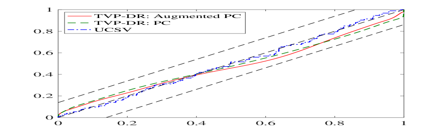
(a) $h=1$

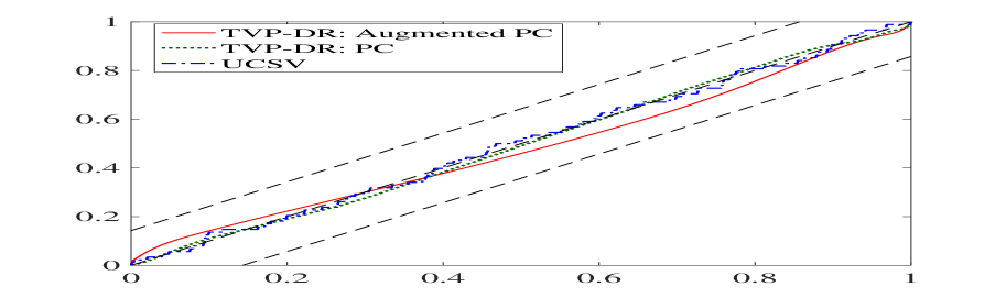
(b) $h=4$

Notes: This figure reports the empirical CDF of the PITs by three models, plus the CDF of the PITs under the null hypothesis of correct calibration (the 45-degree line) and the 95% confidence bands (dashed line) of the Rossi and Sekhposyan (2019) PITs test.

Tails of the inflation distribution are important for studying the inflation risks. We use the quantile scores as a measure to assess the tail forecasting accuracy, which is defined by the following tick loss function,

$$QS_{t}^{h}(\tau):=\big{[}\pi_{t+h}^{h}-\widehat{Q}_{\tau}(\pi_{t+h}^{h}|x_{t})\big{]}1\!{\rm l}\big{\{}\pi_{t+h}^{h}\leq\widehat{Q}_{\tau}(\pi_{t+h}^{h}|x_{t})\big{\}},$$

where $\widehat{Q}_{\tau}(\pi_{t+h}^{h}|x_{t})$ is the estimated $\tau$-th conditional quantile of $\pi_{t+h}^{h}$ at time $t$. Smaller values of the loss function indicate better performance. We compare the quantile scores of the three models for both the 0.05 and 0.95 quantiles, as shown in Figure 2. When $h=1$, the three models perform comparably for both quantiles. However, when $h=4$, for the 0.05 quantile, all the models have comparable good performance during normal periods. In particular, the UCSV outperforms both TVP-DR models during the period when inflation is very low, while the TVP-DR models have better performance when the inflation is excessively high. As for the 0.95 quantile, both TVP-DR models outperform the UCSV model consistently over the entire out-of-sample period. The results for both quantiles show that including more explanatory variables can help to improve the tail forecasting accuracy.

Figure 2: Quantile Scores

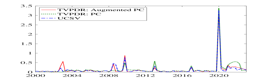
(a) $h=1$: 5%

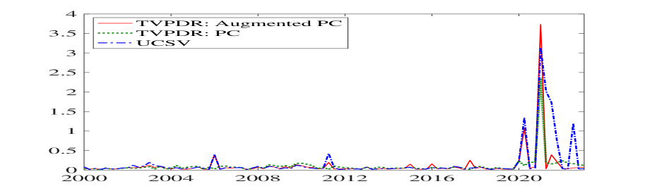
(b) $h=1$: 95%

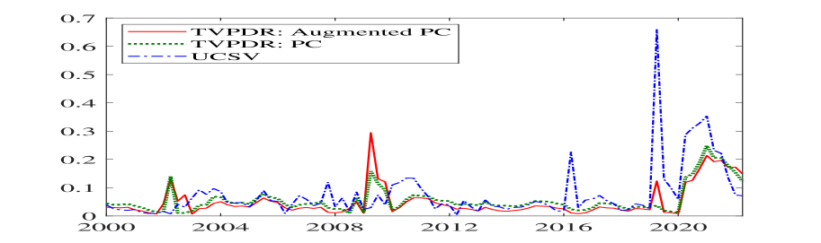
(c) $h=4$: 5%

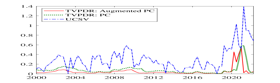
(d) $h=4$: 95%

Notes: This figure plots the 5% and 95% quantile scores computed using three models for horizons $h=1$ and $h=4$.

Therefore, while there has been a lot of evidence for the good performance of UCSV on inflation forecasting, the TVP-DR model is a good alternative for modeling the entire inflation distribution, analyzing the inflation risks, as well as exploring the relationship between inflation and other variables. In the following, with a focus on horizon $h=1$, we study the inflation risks and explore the relationship between the inflation and unemployment rate using the TVP-DR: augmented PC model. For simplicity, in what follows, we denote the $\pi_{t+h}^{h}$ for $h=1$ as $\pi_{t+1}$.

4.3 Inflation Risks

Considering that the TVP-DR model is designed to model the inflation distribution directly, it provides us with a straightforward way to better study different types of inflation risks. In this subsection, based on the TVP-DR: augmented PC model, we analyze the out-of-sample inflation risks that future inflation will be excessively high or low relative to a preferred range. We use risk measures introduced in Kilian and Manganelli (2007), which are designed to make explicit the dependence of risk measures on the private sector agent’s preferences for inflation.

Specifically, let $[\underline{\pi},\bar{\pi}]$ be the preferred range of inflation, where $\underline{\pi}<\bar{\pi}$ are fixed inflation thresholds. According to Kilian and Manganelli (2007), the deflation risk and risk of excessive inflation of $\pi_{t+1}$ are defined as

$$DR_{t}(\underline{\pi},\alpha):=-\int_{-\infty}^{\underline{\pi}}(\underline{\pi}-y)^{\alpha}dF_{\pi|X_{t}}(y|x_{t}),\quad\alpha>0$$

$$EIR_{t}(\bar{\pi},\gamma):=\int_{\bar{\pi}}^{\infty}(y-\bar{\pi})^{\gamma}dF_{\pi|X_{t}}(y|x_{t}),\quad\gamma>0,$$

where $F_{\pi|X_{t}}(y|x_{t})$ is the conditional distribution function of $\pi_{t+1}$ given $X_{t}=x_{t}$, and the parameters $\alpha\geq 0$ and $\gamma\geq 0$ measure the degree of risk aversion of the economic agent. These risk measures provide a unifying framework for several measures of risk proposed in the literature in other contexts, given the flexibility in setting $\alpha$ and $\gamma$. The U.S. Federal Reserve operates under a policy framework known as the “Flexible Inflation Target”, aiming to maintain an inflation rate of 2% over the long run. In this empirical application, we assume that the Fed’s preferred inflation range is between 1% and 3%.

As a start of risk analysis, we present the predictive conditional distributions of inflation in Figure 3. The figure shows the median and the 95% predictive interval of the distribution. Our TVP-DR model demonstrates the ability to capture asymmetries in predictive distributions and accurately predict the evolution of inflation. In addition, the figure reveals potential risks where inflation may exceed the preferred range, particularly during three recession periods. We further explore these risks by examining two special cases of risk measures to quantify them formally. First, we study inflation risks based on risk measures with $\alpha=\gamma=0$, plotted in Panel (a) of Figure 4. In this case, the risk measures reduce to probability of inflation falling below 1% and exceeding 3%, respectively. The results show that our model successfully predicts the significant deflationary likelihood following the early 2000s Recession, the GFC, and COVID, where the GFC has the highest probability of approximately 0.5. In practice, the severe economic downturn and financial instability during the crisis led to a period of deflationary pressures. Importantly, the model captures the rapidly increasing risk of excessive inflation since the pandemic. In addition, it suggests that there were small deflation probabilities, around 0.1, from 2000 to 2010.

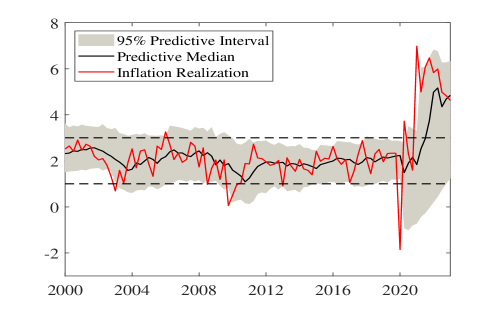
Figure 3: Predictive Distributions of $\pi_{t+1}$

Notes: This figure displays the predicted distributions over time, where the 95% predictive interval (in gray shadow), the predictive mean (in black line), and the true realization (in red line) are plotted. In addition, the preferred range of inflation (1%-3%) is indicated using two parallel black dashed lines.

However, it is important to note that understanding probabilities alone may not be sufficient, as economic agents are typically not indifferent to whether inflation deviates from the target zone by a small or large amount. In this regard, risk measures with $\alpha=\gamma=1$ can provide more meaningful information as they can be interpreted as measures of expected deflation and expected excess inflation. As shown in Panel (b) of Figure 4, the periods identified as having deflation or excessive inflation risks are mostly consistent with the first scenario, while the relative levels of the risks are different. Taking the amount beyond the target range into consideration, the results of the expected deflation suggest certain deflation risks during the GFC and COVID, while the levels are much lower than the risks learned from the deflation probabilities. Except for these two recession periods, both the deflation and excessive inflation risks are negligible. It is particularly noteworthy that the risks from expected excessive inflation indicate a heightened concern about the potential for higher inflation following the pandemic.

Figure 4: Deflation and Excessive Inflation Risks

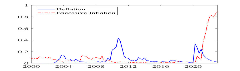
(a) $\alpha=\gamma=0$

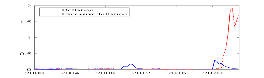
(b) $\alpha=\gamma=1$

Notes: This figure depicts the deflation and excessive inflation risks in two cases. Panel (a) plots the the risk measures when $\alpha=\gamma=0$, which shows the probabilities of inflation falling below 1% (in solid blue line) and exceeding 3% (in dashed red line). Panel (b) plots the the risk measures when $\alpha=\gamma=1$, which shows the expected inflation given it is less than 1% (in solid blue line) or given it is larger than 3% (in dashed red line).

4.4 Relationship between Unemployment and Inflation

The trade-off between unemployment and inflation, often illustrated by the PC, is rooted in the relationship between the labor market and price levels. When unemployment is low, the labor market tightens, and workers can demand higher wages. Companies then spend more on salaries and often raise their prices, leading to inflation. Conversely, when unemployment is high, there is less upward pressure on wages, and inflation tends to be lower. This trade-off is driven by the dynamics of aggregate demand and supply, labor market, and inflation expectations.

Based on the distributional inflation model, we can study the impact of different individual covariates on the distribution functions using the derivative of the distribution function w.r.t the covariates, that is, ${\partial F}/{\partial X_{t}}F_{\pi|X_{t}}(y|X_{t})=\lambda(X_{t}^{\top}\beta_{y,t})\beta_{y,t},$ where $\lambda$ denotes the derivative of the link function $\Lambda$. We first focus on exploring the relationship between the unemployment rate and different segments of the inflation distribution using the partial derivative corresponding to the unemployment gap. Specifically, we analyze two types of inflation risks: the probabilities of inflation being less than 1% and beyond 4%. The corresponding partial derivatives concerning the unemployment gap are illustrated in Figure 5 over time. The findings indicate that there is no substantial association between the unemployment rate and inflation risks during normal economic periods. However, during periods characterized by risks, we observe a positive correlation between unemployment and deflation risk, coupled with a negative correlation with the risk of excessive inflation.

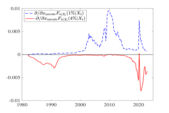
Figure 5: The Effect of Unemployment Gap on Inflation Risks

Notes: This figure plots the partial derivatives of $F_{\pi|X_{t}}(1\%|X_{t})$(in blue dashed line) and $1-F_{\pi|X_{t}}(4\%|X_{t})$ (in red solid line) with respect to the unemployment gap ($x_{unrate}$) over time.

Additionally, we conduct a counterfactual analysis encompassing the GFC and the COVID periods to examine the potential impact of adjusting the quarterly unemployment gap on the overall inflation distribution. Specifically, utilizing the model estimated with the entire sample, we explore the changes in the inflation distribution when the unemployment gap is reduced by 5% in each quarter from 2009:Q1 to 2009:Q4 and increased by 5% in each quarter from 2021:Q1 to 2021:Q4. Table 1 displays the realized and counterfactual unemployment gap for these periods, while Figure 6 illustrates the baseline and counterfactual inflation distributions in each quarter.

Table 1: True and Modified Unemployment Gap (%)

GFC		2009:Q1	2009:Q2	2009:Q3	2009:Q4
	Realized	3.39	4.43	4.77	5.08
	Counterfactual	-1.61	-0.57	-0.23	0.08
COVID		2021:Q1	2021:Q2	2021:Q3	2021:Q4
	Realized	1.73	1.47	0.68	-0.25
	Counterfactual	6.73	6.47	5.68	4.75

Notes: This table displays the actual unemployment gap for each quarter during the GFC and COVID, alongside the adjusted values used in our counterfactual analysis.

From the first column in Figure 6, initially, in 2009:Q1, the baseline distribution of inflation was asymptotically symmetrical, in the following three quarters, the distribution became increasingly right-skewed. A counterfactual experiment involving a reduction in the unemployment gap by 5% in 2009:Q1 has a limited immediate impact on the forecasting distribution of inflation. This suggests that, during the immediate post-GFC period, monetary policy measures and broader economic dynamics played more dominant roles in shaping inflation expectations. Nevertheless, after 2009:Q1, if there was a reduction in the unemployment gap, the forecasting distribution became much less skewed, with a noteworthy reduction in the left tail probability ($\pi_{t+1}<1\%$), indicating that as the economy stabilized and the impact of monetary policy became clearer, inflation expectations adjusted, reducing deflationary concerns. As shown in the second column in Figure 6, an examination of inflation distributions uncovered left-skewed patterns, reflecting the abrupt demand and supply shocks caused by the pandemic and the ensuing economic uncertainty. Counterfactual analyses involving increases in the unemployment gap by 5% during these periods led to a noteworthy observation: the forecasting distribution of inflation became less left-skewed, with a decrease in the right tail probability ($\pi_{t+1}>5\%$). This suggests that policies aimed at mitigating unemployment could contribute to stabilizing economic conditions and alleviating deflationary concerns during this crisis.

Figure 6: The Effect of Unemployment Gap on Inflation Distribution

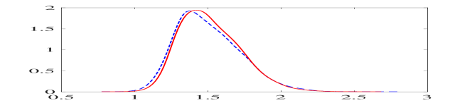
(a) 2009: Q1

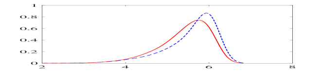
(b) 2021: Q1

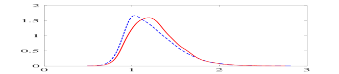
(c) 2009: Q2

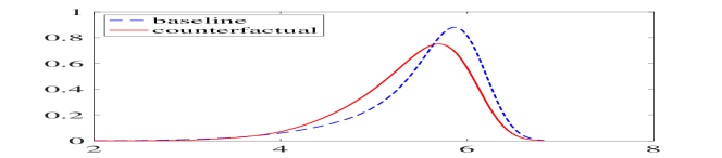
(d) 2021: Q2

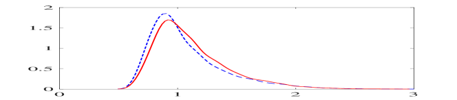
(e) 2009: Q3

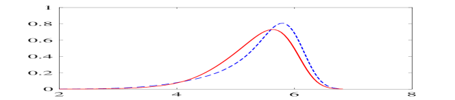
(f) 2021: Q3

(g) 2009: Q4

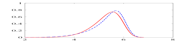
(h) 2021: Q4

Notes: This figure plots the baseline (in blue dashed line) and counterfactual (in red solid line) inflation distributions following the GFC (first column) if we decrease the unemployment gap in each quarter from 2009:Q1-Q4 by 5% and the COVID (second column) if we increase the unemployment gap in each quarter from 2021:Q1-Q4 by 5%.

4.5 Up-to-date Forecasting and Analysis

In economic history, there have been instances where governments or central banks have implemented policies that could potentially lead to higher unemployment in an effort to control high inflation. For example, in the late 1970s, the U.S. faced a big problem with high inflation, partly due to rising oil prices. The CPI went up to about 13.5% in 1980. To fight this high inflation, the Fed started a series of tight monetary policies that greatly increased interest rates. While these policies succeeded in reducing inflation, they came at a significant cost in terms of higher unemployment with the unemployment rate peaking at around 10.8% in 1982. During the Eurozone debt crisis, countries like Greece and Spain also dealt with high inflation, with Greece’s rate going over 4% in 2008 and 2009. The European Central Bank responded with strict budget policies and higher interest rates. These actions caused economic downturns and big increases in unemployment, with Greece’s unemployment rate going over 27% in 2013.

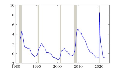
Figure 7: Historial Unemployment Gap

Notes: The shaded bars indicate the historical recessions in the U.S..

In the following, we embark on a comprehensive study of inflation dynamics in the latest quarter, 2023:Q3, given the available covariates information in 2023:Q2. Utilizing our proposed model, we forecast the distribution of inflation in 2023:Q3 and undertake a counterfactual analysis to investigate how inflation responds to policy measures resulting in a substantial increase in the unemployment gap. As shown in Figure 7, in the U.S., significant economic downturns, such as the recessions in 1982 and 2009, witnessed unemployment gaps hovering around 4%-5%. Therefore, given the true unemployment gap of -0.86% in 2023:Q3, we consider a 5% increase in the unemployment gap as a significant and challenging level that policymakers can potentially accept in their pursuit of reducing the inflation rate. In this case, the unemployment rate is around 8.6%, given the natural unemployment rate at 4.42%. The baseline and counterfactual forecasts for the distribution of inflation in 2023:Q3 are visualized in Figure 8, while Table 2 presents the associated probabilities of inflation exceeding a range of predetermined thresholds.

Table 2: Effect of Increasing Unemployment Gap on Inflation in 2023:Q3

Measures Mean $P(\pi_{t+1}>3\%)$ $P(\pi_{t+1}>4\%)$ $P(\pi_{t+1}>5\%)$ $P(\pi_{t+1}>6\%)$ Baseline 4.6270 0.9696 0.8361 0.3171 0.0084 Counterfactual 4.5424 0.9767 0.8346 0.2273 0.0034 Notes: This table presents the mean and different probabilities of inflation in 2023:Q3, and their counterfactual counterparts with a 5% increase in the unemployment gap.

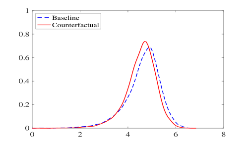
Figure 8: Inflation Distribution in 2023:Q3

Notes: This figure plots the baseline (in blue dashed line) and counterfactual (in red solid line) inflation distributions in 2023:Q3, with a 5% increase in the unemployment gap.

The findings reveal that introducing a 5% increase in the unemployment gap exhibits a modest effect, marginally reducing the likelihood of inflation beyond 4%. However, noteworthy is the absence of a significant impact on the left tail and the predictive mean of inflation. Our analysis underscores that while a high unemployment rate of 8.2% can exert a marginal dampening effect on the probability of exceptionally high inflation, there remains a substantial journey ahead to steer inflation back into the desired target range.

5 Conclusion

This paper introduces a TVP-DR model for analyzing the full conditional distribution of inflation. This model represents a significant leap from the traditional DR method, accommodating the dynamic nature of financial markets and macroeconomic trends. By integrating a precision-based MCMC algorithm, our approach efficiently handles the complexities inherent in estimating time-varying parameters, offering a more computationally viable alternative to standard methods. In addition, we introduce an efficient algorithm that ensures the monotonicity condition on the conditional distribution function directly within the estimation process. This advancement overcomes the limitations of the two-step procedures commonly used in the DR and QR literature, ensuring a more integrated approach in Bayesian inference.

The TVP-DR model marks a substantial contribution to understanding inflation dynamics. In contrast to numerous inflation risk studies concentrating on lower and upper quantiles, our model provides a straightforward way to explore inflation risks concerning a target range specified by the central bank and how various covariates influence these risks. Our empirical analysis investigates U.S. inflation conditional on a comprehensive set of macroeconomic and financial indicators. A thorough examination of the intricate relationship between the unemployment rate and the dynamics of inflation risks and distributions is provided. In our up-to-date analysis, we explore a scenario wherein policymakers are willing to tolerate a relatively high unemployment cost to address high inflation. This exploration yields valuable insights into the potential challenges policymakers may encounter while navigating the balance between inflation control and managing unemployment in the contemporary economic landscape.

Appendix A Data Appendix

In this section, we provide details on the inflation data and covariates used.

A.1 Inflation

Consumer Price Index ($P_{t}$): Consumer Price Index for all urban consumers: all items less food and energy (1982-84=100). Source: FRED-QD database, ‘CPILFESL’.

Figure A.1: CPI Inflation $\pi_{t+h}^{h}$ for $h=4$

Notes: $\pi_{t+h}^{h}=(400/h)\ln(P_{t+h}/P_{t})$

A.2 Covariates

• Four inflation determinants in PC model of Blanchard et al. (2015):

  • Long-term Inflation Expectation $(\pi_{t}^{LTE})$: 10-year expected inflation, Percent, Quarterly, Not Seasonally Adjusted. Source: FRED, ‘EXPINF10YR’.

  • Unemployment Rate $(u_{t})$: Civilian Unemployment Rate, Percent, Quarterly, Seasonally Adjusted. Source: FRED, ‘UNRATE’.

  • Natural Rate of Unemployment $(u_{t}^{*})$: Noncyclical Rate of Unemployment, Percent, Quarterly, Not Seasonally Adjusted. Source: FRED, ‘NROU’.

  • Import Price Index: Imports of goods and services (chain-type price index), Continuously Compounded Annual Rate of Change, Quarterly, Seasonally Adjusted. Source: FRED, ‘B021RG3Q086SBEA_CCA’.

• Six additional covariates from the FRED-QD database of McCracken and Ng (2020): The last column of Table A.1 denotes one of the following transformations applied for the original series $x_{t}$: 1-No transformation, 2-$\Delta x_{t}$, 3-$\Delta^{2}x_{t}$, 4-$\log(x_{t})$, 5-$\Delta\log(x_{t})$, 6-$\Delta^{2}\log(x_{t})$.

  Table A.1: Additional Covariates from FRED-QD

  Variable Label	Description	Trans
  AWHMAN	Average Weekly Hours of Production and Nonsupervisory Employees: Manufacturing (Hours)	1
  PPIACO	Producer Price Index for All Commodities	6
  ULCNFB	Nonfarm Business Sector: Unit Labor Cost (Index 2012-100)	5
  S&P 500	S&P’s Common Stock Price Index: Composite	5
  FEDFUNDS	Effective Federal Funds Rates (Percent)	2
  GDPC1	Real Gross Domestic Product	5
  M2REAL	Real M2 Money Stock	5

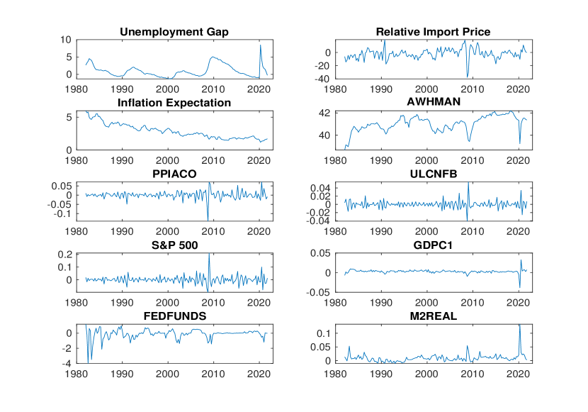
Figure A.2: Covariates

References

- Adrian et al. (2019) Adrian, T., N. Boyarchenko, and D. Giannone (2019). Vulnerable growth. American Economic Review 109(4), 1263–89.
- Albert and Chib (1993) Albert, J. H. and S. Chib (1993). Bayesian analysis of binary and polychotomous response data. Journal of the American Statistical Association 88(422), 669–679.
- Banerjee et al. (2024) Banerjee, R., J. Contreras, A. Mehrotra, and F. Zampolli (2024). Inflation at risk in advanced and emerging market economies. Journal of International Money and Finance, 103025.
- Belmonte et al. (2014) Belmonte, M. A., G. Koop, and D. Korobilis (2014). Hierarchical shrinkage in time-varying parameter models. Journal of Forecasting 33(1), 80–94.
- Blanchard et al. (2015) Blanchard, O., E. Cerutti, and L. Summers (2015). Inflation and activity–two explorations and their monetary policy implications. Technical report, National Bureau of Economic Research.
- Blanchard and Bernanke (2023) Blanchard, O. J. and B. S. Bernanke (2023). What caused the US pandemic-era inflation? Technical report, National Bureau of Economic Research.
- Bondell et al. (2010) Bondell, H. D., B. J. Reich, and H. Wang (2010). Noncrossing quantile regression curve estimation. Biometrika 97(4), 825–838.
- Botev (2017) Botev, Z. I. (2017). The normal law under linear restrictions: simulation and estimation via minimax tilting. Journal of the Royal Statistical Society Series B: Statistical Methodology 79(1), 125–148.
- Carter and Kohn (1994) Carter, C. K. and R. Kohn (1994). On Gibbs sampling for state space models. Biometrika 81(3), 541–553.
- Chan (2017) Chan, J. C. (2017). The stochastic volatility in mean model with time-varying parameters: An application to inflation modeling. Journal of Business & Economic Statistics 35(1), 17–28.
- Chan (2023) Chan, J. C. (2023). Large hybrid time-varying parameter VARs. Journal of Business & Economic Statistics 41(3), 890–905.
- Chan and Jeliazkov (2009) Chan, J. C. and I. Jeliazkov (2009). Efficient simulation and integrated likelihood estimation in state space models. International Journal of Mathematical Modelling and Numerical Optimisation 1(1-2), 101–120.
- Chan et al. (2023) Chan, J. C., D. Pettenuzzo, A. Poon, and D. Zhu (2023). Conditional Forecasts in Large Bayesian VARs with Multiple Soft and Hard Constraints. Technical report.
- Chernozhukov et al. (2009) Chernozhukov, V., I. Fernandez-Val, and A. Galichon (2009). Improving point and interval estimators of monotone functions by rearrangement. Biometrika 96(3), 559–575.
- Chernozhukov et al. (2013) Chernozhukov, V., I. Fernández-Val, and B. Melly (2013). Inference on counterfactual distributions. Econometrica 81(6), 2205–2268.
- Clark and Ravazzolo (2015) Clark, T. E. and F. Ravazzolo (2015). Macroeconomic forecasting performance under alternative specifications of time-varying volatility. Journal of Applied Econometrics 30(4), 551–575.
- Cogley and Sargent (2005) Cogley, T. and T. J. Sargent (2005). Drifts and volatilities: monetary policies and outcomes in the post WWII US. Review of Economic Dynamics 8(2), 262–302.
- Das and Ghosal (2018) Das, P. and S. Ghosal (2018). Bayesian non-parametric simultaneous quantile regression for complete and grid data. Computational Statistics & Data Analysis 127, 172–186.
- Dette and Volgushev (2008) Dette, H. and S. Volgushev (2008). Non-crossing non-parametric estimates of quantile curves. Journal of the Royal Statistical Society Series B: Statistical Methodology 70(3), 609–627.
- Durbin and Koopman (2002) Durbin, J. and S. J. Koopman (2002). A simple and efficient simulation smoother for state space time series analysis. Biometrika 89(3), 603–616.
- Foresi and Peracchi (1995) Foresi, S. and F. Peracchi (1995). The conditional distribution of excess returns: An empirical analysis. Journal of the American Statistical Association 90(430), 451–466.
- Frühwirth-Schnatter and Wagner (2010) Frühwirth-Schnatter, S. and H. Wagner (2010). Stochastic model specification search for Gaussian and partial non-Gaussian state space models. Journal of Econometrics 154(1), 85–100.
- Gallant et al. (2017) Gallant, A. R., R. Giacomini, and G. Ragusa (2017). Bayesian estimation of state space models using moment conditions. Journal of Econometrics 201(2), 198–211.
- Giacomini and Levin (2023) Giacomini, R. and Y. Levin (2023). Microforecasting inflation. Economic Perspectives (3).
- Hauzenberger et al. (2022) Hauzenberger, N., F. Huber, G. Koop, and L. Onorante (2022). Fast and flexible Bayesian inference in time-varying parameter regression models. Journal of Business & Economic Statistics 40(4), 1904–1918.
- Holmes and Held (2006) Holmes, C. C. and L. Held (2006). Bayesian auxiliary variable models for binary and multinomial regression. Bayesian Analysis 1(1), 145–168.
- Kilian and Manganelli (2007) Kilian, L. and S. Manganelli (2007). Quantifying the risk of deflation. Journal of Money, Credit and Banking 39(2-3), 561–590.
- Koop (2003) Koop, G. (2003). Bayesian econometrics. Wiley.
- Koop and Korobilis (2012) Koop, G. and D. Korobilis (2012). Forecasting inflation using dynamic model averaging. International Economic Review 53(3), 867–886.
- Koop and Korobilis (2013) Koop, G. and D. Korobilis (2013). Large time-varying parameter VARs. Journal of Econometrics 177(2), 185–198.
- Korobilis (2017) Korobilis, D. (2017). Quantile regression forecasts of inflation under model uncertainty. International Journal of Forecasting 33(1), 11–20.
- Korobilis et al. (2021) Korobilis, D., B. Landau, A. Musso, and A. Phella (2021). The time-varying evolution of inflation risks. Technical report.
- Kozumi and Kobayashi (2011) Kozumi, H. and G. Kobayashi (2011). Gibbs sampling methods for Bayesian quantile regression. Journal of Statistical Computation and Simulation 81(11), 1565–1578.
- Liu and Wu (2011) Liu, Y. and Y. Wu (2011). Simultaneous multiple non-crossing quantile regression estimation using kernel constraints. Journal of Nonparametric Statistics 23(2), 415–437.
- Lopez-Salido and Loria (2020) Lopez-Salido, D. and F. Loria (2020). Inflation at Risk. Technical report.
- Marcellino et al. (2023) Marcellino, M., T. Clark, F. Huber, and G. Koop (2023). Forecasting US Inflation Using Bayesian Nonparametric Models. Technical report, CEPR Discussion Papers.
- McCracken and Ng (2020) McCracken, M. and S. Ng (2020). FRED-QD: A quarterly database for macroeconomic research. Technical report, National Bureau of Economic Research.
- Medeiros et al. (2021) Medeiros, M. C., G. F. Vasconcelos, Á. Veiga, and E. Zilberman (2021). Forecasting inflation in a data-rich environment: the benefits of machine learning methods. Journal of Business & Economic Statistics 39(1), 98–119.
- Mitchell et al. (2022) Mitchell, J., A. Poon, and D. Zhu (2022). Constructing Density Forecasts from Quantile Regressions: Multimodality in Macro-Financial Dynamics. Technical report.
- Nakajima (2011) Nakajima, J. (2011). Time-varying parameter model with stochastic volatility: An overview of methodology and empirical applications. Monetary and Economic Studies 29.
- Pfarrhofer (2022) Pfarrhofer, M. (2022). Modeling tail risks of inflation using unobserved component quantile regressions. Journal of Economic Dynamics and Control 143, 104493.
- Polson et al. (2013) Polson, N. G., J. G. Scott, and J. Windle (2013). Bayesian inference for logistic models using Pólya–Gamma latent variables. Journal of the American Statistical Association 108(504), 1339–1349.
- Primiceri (2005) Primiceri, G. E. (2005). Time varying structural vector autoregressions and monetary policy. The Review of Economic Studies 72(3), 821–852.
- Qu and Yoon (2015) Qu, Z. and J. Yoon (2015). Nonparametric estimation and inference on conditional quantile processes. Journal of Econometrics 185(1), 1–19.
- Rodrigues and Fan (2017) Rodrigues, T. and Y. Fan (2017). Regression adjustment for noncrossing Bayesian quantile regression. Journal of Computational and Graphical Statistics 26(2), 275–284.
- Rossi and Sekhposyan (2019) Rossi, B. and T. Sekhposyan (2019). Alternative tests for correct specification of conditional predictive densities. Journal of Econometrics 208(2), 638–657.
- Stock and Watson (1996) Stock, J. H. and M. W. Watson (1996). Evidence on structural instability in macroeconomic time series relations. Journal of Business & Economic Statistics 14(1), 11–30.
- Stock and Watson (1999) Stock, J. H. and M. W. Watson (1999). Forecasting inflation. Journal of Monetary Economics 44(2), 293–335.
- Stock and Watson (2007) Stock, J. H. and M. W. Watson (2007). Why has US inflation become harder to forecast? Journal of Money, Credit and Banking 39, 3–33.
- Wang et al. (2023) Wang, Y., T. Oka, and D. Zhu (2023). Distributional Vector Autoregression: Eliciting Macro and Financial Dependence. Technical report, arXiv. org.
- Williams and Grizzle (1972) Williams, O. D. and J. E. Grizzle (1972). Analysis of contingency tables having ordered response categories. Journal of the American Statistical Association 67(337), 55–63.