INSIGHT: End-to-End Neuro-Symbolic Visual Reinforcement Learning with Language Explanations

Abstract

Neuro-symbolic reinforcement learning (NS-RL) has emerged as a promising paradigm for explainable decision-making, characterized by the interpretability of symbolic policies. For tasks with visual observations, NS-RL entails structured representations for states, but previous algorithms are unable to refine the structured states with reward signals due to a lack of efficiency. Accessibility is also an issue, as extensive domain knowledge is required to interpret current symbolic policies. In this paper, we present a framework that is capable of learning structured states and symbolic policies simultaneously, whose key idea is to overcome the efficiency bottleneck by distilling vision foundation models into a scalable perception module. Moreover, we design a pipeline that uses large language models to generate concise and readable language explanations for policies and decisions. In experiments on nine Atari tasks, our approach demonstrates substantial performance gains over existing NSRL methods. We also showcase explanations for policies and decisions.

1 Introduction

Recent years have witnessed remarkable progress in the field of deep reinforcement learning (RL) (Agarwal et al., 2021; Wurman et al., 2022; Degrave et al., 2022). However, deep RL still faces limitations in sensitive domains due to its opaque nature (Milani et al., 2022). Neuro-symbolic reinforcement learning (NS-RL) is promising for overcoming the limitations (Verma et al., 2018; Coppens et al., 2019). In its simplest form, NS-RL represents policies with expressions over quantities related to objects, such as polynomials of object locations. The interpretability of an agent’s decision-making process is thus guaranteed by the clear semantics and concise formulation of the policies.

For tasks with visual observations, NS-RL entrails structured state representations consisting of object locations, which means to map input pixels to objects. Zheng et al. (2022) proposed to extract the structured states from the Spatially Parallel Attention and Component Extraction (SPACE) model (Lin et al., 2020) trained on task-specific data. However, the state representations are fixed during policy learning due to the computational overhead of SPACE. That being said, the structured states are not refined with reward signals, which can lead to a significant loss in task performance.

Meanwhile, symbolic policies can be intricate for general users, albeit being intrinsically interpretable. For instance, to interpret logical policies (Delfosse et al., 2023a) one has to be familiar with first-order logic, and for programmatic policies (Qiu & Zhu, 2022) one has to learn the corresponding grammars. From a practical point of view, it is imperative to attain accessibility to the general public in order to gain their trust. Nevertheless, there is a lack effort in the literature of NS-RL to make policy interpretations for non-expert users.

In this paper, we present a framework called INSIGHT (INSIGHT) to address these issues. As illustrated in Fig. 1, INSIGHT is able to learn the object coordinates and symbolic policies simultaneously, and it can explain learned policies and specific decisions in natural language. The key idea for learning structured states is to distill vision foundation models into a scalable perception module that overcomes the efficiency drawback of previous approaches. We use the equation learner (EQL) (Sahoo et al., 2018) for learning symbolic policies from object coordinates, which allows both the perception module and the symbolic policy to be trained with rewards.

Moreover, we develop a pipeline for explaining policies and decisions in natural language using large language models (LLMs), which reduces the cognitive load on users to understand the construction of symbolic policies learned by INSIGHT. Through a step called concept grounding, we help LLMs to associate general concepts such as objects and motions with variables in the symbolic policies. Then, as illustrated in Fig. 1, LLMs are instruct to interpret the general patterns of decision-making based on the expressions of symbolic policies and specific decision based on specific values of object coordinates.

We verify the efficacy of INSIGHT and its model design with extensive experiments on nine Atari games. INSIGHT outperforms all existing approaches for NS-RL (CGP (Wilson et al., 2018), Diffses (Yuan et al., 2022), DSP (Landajuela et al., 2021), and NUDGE (Delfosse et al., 2023a)). We show that its empirical performance can be attributed to the refinement of structured states with reward information and our approach for learning symbolic policies. We also present examples of policy interpretations and decision explanations. In summary, our contributions are three-fold.

1. We propose an NS-RL framework that can refine structured states with both visual and reward information.

2. We develop a pipeline for explaining symbolic policies in natural languages.

3. We demonstrate the efficacy of INSIGHT on nine Atari games and showcase its policy explanations.

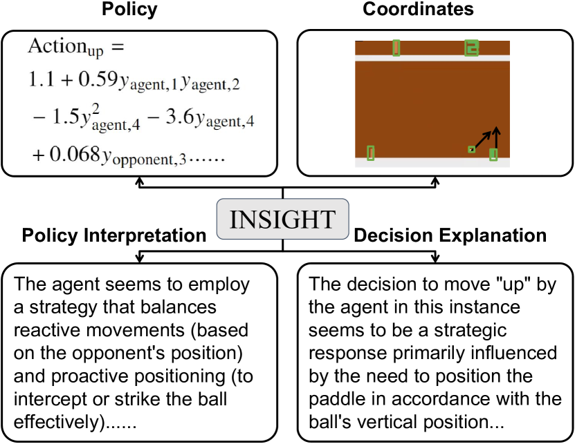
Figure 1: For tasks with visual input, INSIGHT can simultaneously learn the coordinates of objects in observations and coordinate-based symbolic policies simultaneously, and it can interpret learned policies and specific decisions in natural language.

2 Related work

Approaches for explainable RL can be categorized into post hoc and intrinsic methods. The former generates explanations using predefined templates (Ehsan et al., 2018; Wang et al., 2019; Hayes & Shah, 2017) or saliency maps (Greydanus et al., 2018) but can be subjective and unreliable (Dazeley et al., 2023). The latter relies on interpretable function approximators, such as decision trees (Topin et al., 2021; Zhang et al., 2021), for better transparency, yet they often suffer from limited performance due to non-differentiability (Dazeley et al., 2023).

Approaches for NS-RL are intrinsically interpretable due to the construction of symbolic policies. Most existing approaches focus on tasks with low-dimensional observations that have clear semantics (Verma et al., 2018; Coppens et al., 2019; Verma et al., 2019; Landajuela et al., 2021). For tasks with visual input, they either rely on ground truth (Delfosse et al., 2023a) or human-defined primitives (Wilson et al., 2018; Lyu et al., 2019) for state representations. As an exception, Zheng et al. (2022) proposed to extract structured states from pre-trained SPACE models, yet the representations are not refined with reward signals. To our knowledge, INSIGHT is the first framework that learns structured states from both visual and reward signals.

Meanwhile, there is a growing interest in using LLMs to explain machine learning models. For instance, Kroeger et al. (2023) leveraged LLMs to rank features by their importance, and Tennenholtz et al. (2023) used LLMs to explain latent embeddings. INSIGHT is related to the approaches that generate explanations based on input-output pairs (Singh et al., 2023; Bills et al., 2023) or decision trees distilled from the neural models (Zhang et al., 2023). However, INSIGHT is able to prompt LLMs with the actual symbolic policies due to their simplicity and generate more informed explanations.

3 INSIGHT

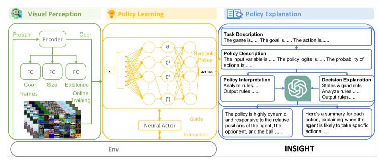
Figure 2: INSIGHT consists of three components: a perception module, a policy learning module, and a policy explanation module. The perception module learns to predict object coordinates using a frame-symbol dataset distilled from vision foundation models. The policy learning module is responsible for learning coordinate-based symbolic policies. In particular, to address with the limited expressiveness of object coordinates, it uses a neural actor to interact with the environment. The policy explanation module can generate policy interpretations and decision explanations using task description, policy description, and values of object coordinates.

This section presents the proposed INSIGHT framework. As illustrated in Fig. 2, it consists of three components: a visual perception module (Sec. 3.1), a policy learning module (Sec. 3.2), and a policy explanation module (Sec. 3.3).

3.1 Visual Perception

Frame-Symbol Dataset  The perception module needs to extract information about objects from input images. Given the notorious sample efficiency of online RL, approaches that use image reconstruction objectives (Zheng et al., 2022; Yoon et al., 2023) are prohibitively expansive. We claim that, for NSRL, compared to reproducing every detail in visual observations, it suffices to only recognize the positions of objects. To this end, we consider harvesting the segmentation and tracking ability of vision foundation models. For each task, we first roll out about 10,000 observations using pre-trained neural agents, and then we extract the bounding boxes of objects in these observations using the FastSAM segmentation model (Zhao et al., 2023) and the DeAot model (Yang & Yang, 2022). Using the bounding boxes, we compute the coordinates of objects (i.e., their centers) and their shape, normalize them to $[0,1]$, and pair them with the corresponding images to form a frame-symbol dataset $\mathcal{D}_{\text{symbol}}$. Details of the dataset generation are provided in Sec. A.1. By fitting to this dataset, the perception module extract the structured states efficiently, a critical condition of refining them during policy learning.

Learning Object Coordinates  We now present the details of learning from $\mathcal{D}_{\text{symbol}}$. $\mathcal{D}_{\text{symbol}}$ contains information of the existence, the shape, and the coordinates of objects. To make full use of them, INSIGHT employs a multi-task formulation for the perception module $\omega_{\text{perception}}$, which is illustrated in Fig. 2. An encoder, parameterized by convolutional neural networks (CNNs) and FCNs, is responsible for encoding information about objets and rewards into hidden representations. Three FCNs use the hidden representations to predict the existence, the shape, and the coordinates of objects, which are explained below.

Objects can appear and disappear in many tasks. Only the coordinates of present objects can be used by the symbolic policy, otherwise it will exploit the coordinates of missing objects and lose interpretability. Therefore, we need to mask out the coordinates of missing objects during policy learning, which requires predicting the existence of objects. One issue of existence prediction is that the distribution of objects can be long tailed. For example, in the BeamRider task, the agent’s spaceship is present at almost every step, while torpedoes appear less frequently. This issue is handled with the distribution-balanced focal loss (Wu et al., 2020).

Specifically, for the $j$^th object in the $i$^th sample, let $c_{ij}=1$ if it is present, and $c_{ij}=0$ otherwise. Let $C$ be the number of objects and $N$ be the number of samples. This loss extend the focal loss (Lin et al., 2017) by weighting labels with their inverse frequency. It is given by

$$\mathcal{L}_{\mathrm{exist}}=-\frac{1}{N}\sum_{i=1}^{N}\sum_{j=1}^{C}\bar{\eta}_{ij}\Big{[} c_{ij}(1-p_{ij})^{\psi}\log(p_{ij})$$ (1)

$$+(1-c_{ij}) p_{ij}^{\psi}\log(1-p_{ij})\Big{]},$$

where $\psi$ is the modulating factor of the focal loss (Lin et al., 2017). Details for computing $\bar{\eta}_{ij}$ is provided in Sec. A.2.

As for coordinate prediction, we use the L1 loss since the normalized coordinates can take small values. Let $\mathbf{x}_{i}\in\mathbb{R}^{2C}$ be the vector for object coordinates in the $i$^th image and $\mathbf{\hat{x}}_{i}$ be its predicted value. For $j=1,2,\dots,C$, $x_{i,2j}$ and $x_{i,2j+1}$ is the Y and X coordinate for the $j$^th object. Then, the objective for coordinate prediction is given by:

$$\mathcal{L}_{\mathrm{coor}}=\frac{1}{N}\sum_{i=1}^{N}\sum_{j=1}^{C}c_{ij}\left[\left|x_{i,2j}-\hat{x}_{i,2j}\right|+\left|x_{i,2j+1}-\hat{x}_{i,2j+1}\right|\right].$$ (2)

Note that the predicted coordinates are clipped to $[0,1]$ when being used for policy learning, as they are supposed to be the coordinates of objects. For shape prediction, the network is trained to predict the width and height of object bounding boxes. The loss, $\mathcal{L}_{\mathrm{size}}$, takes a similar form as $\mathcal{L}_{\mathrm{coor}}$, except that the prediction targets are replaced with the width and height of objects. Overall, the objective for learning from the frame-symbol dataset is:

$$\mathcal{L}_{\mathrm{cnn}}=\mathcal{L}_{\mathrm{exist}}+\mathcal{L}_{\mathrm{coor}}+\mathcal{L}_{\mathrm{size}}.$$ (3)

Before policy learning, the perception module is pre-trained on frame-symbol datasets to equips agents with knowledge about objects. We will verify this design choice in Sec. 4.

3.2 Learning Symbolic Policies

EQL  We represent symbolic policies with the EQL network (Martius & Lampert, 2016; Sahoo et al., 2018). Given an input vector $\mathbf{h}^{(k-1)}\in\mathbb{R}^{d_{k-1}}$, its $k$^th layer first applies a transformation $\mathbf{g}^{(k)}=\mathbf{W}^{(k)}\mathbf{h}^{(k-1)}+\mathbf{b}^{(k)}$, where $\mathbf{W}^{(k)}\in\mathbb{R}^{d_{k}\times d_{k-1}}$ and $\mathbf{b}^{(k)}\in\mathbb{R}^{d_{k}}$ are learnable parameters. $d_{k-1}$ and $d_{k}$ are the dimension of $\mathbf{h}^{(k-1)}$ and $\mathbf{g}^{(k)}$.

Compared to fully-connected layers (FCN), EQL has more flexible activation functions. The activation function for a vector $\mathbf{g}\in\mathbb{R}^{d_{k}}$, $\mathbf{f}:\mathbb{R}^{d_{k}}\to\mathbb{R}^{d^{\prime}_{k}}$, is given by

$$\mathbf{f}(\mathbf{g})=\left[\begin{array}[]{c}f_{1}(g_{1})\\ \vdots\\ f_{u}(g_{u})\\ f_{u+1}(g_{u+1},g_{u+2})\\ \vdots\\ f_{d^{\prime}_{k}}(g_{d_{k}-1},g_{d_{k}})\end{array}\right],$$ (4)

where $f_{1}$, $f_{2}$, …, $f_{d^{\prime}_{k}}\in\mathcal{F}$ are scalar functions. $f_{1},f_{2},\dots,f_{u}$ are unary functions, and the remaining are binary functions. EQL networks are often much smaller than FCNs to enhance interpretability. It is the flexibility of activation functions that enhances expressiveness. In this work, $\mathcal{F}$ includes the square function, the cubic function, constants, the identity function, multiplication, and addition.

The final ingredient is sparsity regularization (Martius & Lampert, 2016) required for deriving concise expressions, which imposes the following regularization to the parameters of a EQL network to avoid the singularity in the gradient as the weights go to 0.

$$\mathcal{L}_{\text{reg}}(w)=\begin{cases}|w|^{1/2}&|w|\geq a\\ \left(-\frac{w^{4}}{8a^{3}}+\frac{3w^{2}}{4a}+\frac{3a}{8}\right)^{1/2}&|w|<a\end{cases}$$ (5)

Here, $a=0.05$ is a smoothing parameter.

Algorithm 1 Procedures for learning symbolic policy

  Input: Pretrained perception module $\omega_{\text{perception}}$ and the frame-symbol dataset $\mathcal{D}_{\text{symbol}}$

  Output: Fine-tuned perception module and the EQL actor $\pi_{\text{EQL}}$

  Initialize the neural actor $\pi_{\text{nerual}}$ and the EQL actor $\pi_{\text{EQL}}$ randomly.

  for batch = $1,2,\ldots$ do

    Collect online samples $\mathcal{D}_{\text{batch}}$ using $\pi_{\text{nerual}}$.

    for iteration=$n$ do

       if $x_{i}>x_{i+1}$ then

          Update $\pi_{\text{nerual}}$, $\pi_{\text{EQL}}$, and $\omega_{\text{perception}}$ by minimizing $\mathcal{L}$ using $\mathcal{D}_{\text{batch}}$ and $\mathcal{D}_{\text{symbol}}$.

       else

          Update $\pi_{\text{neural}}$ and $\omega_{\text{perception}}$ by minimizing $\mathcal{L}_{\text{ppo}}$ using $\mathcal{D}_{\text{batch}}$.

       end if

    end for

  end for

Neural Guidance We now discuss the challenges in learning symbolic policies. The symbolic policy, referred to as the EQL actor $\pi_{\text{EQL}}$, computes action distributions using the predicted object coordinates. While being intuitive, it is worth noting that the object coordinates $\mathbf{x}$ are subject to limited expressiveness. Each element of $\mathbf{x}$ is bound to the Y or X coordinate of some objects, which means they are not distributed representations and cannot encode complex patterns as neural representations do. What exacerbates the situation is that the expressions represented by $\pi_{\text{EQL}}$ are forced to be concise by $\mathcal{L}$. In consequence, $\pi_{\text{EQL}}$ might not be able to represent all possible policies and fail to explore well during policy learning.

We therefore opt for using $\pi_{\text{EQL}}$ to approximate only the optimal policy, which is less demanding than approximating all possible policies. Inspired by Nguyen et al. (2021); Landajuela et al. (2021), we propose a neural guidance scheme that uses a neural actor $\pi_{\text{neural}}$ to interact with the environment. $\pi_{\text{neural}}$ takes as input the hidden representations produced by the encoder of $\omega_{\text{perception}}$ and is not regularized by $\mathcal{L}_{\text{0.5}}$, so it can effectively explore the state-action space. The EQL actor is trained to distill $\pi_{\text{neural}}$ using symbolic expressions and coordinate. Compared to existing neural guidance schemes (Nguyen et al., 2021; Landajuela et al., 2021), in our scheme the EQL actor and the neural actor are trained simultaneously rather than separately, which results in improved sample efficiency.

The procedures for learning symbolic policies are outlined in Alg. 1. Specifically, we optimize the neural actor using the Proximal Policy Optimization (PPO) (Schulman et al., 2017) algorithm, whose objective is denoted by $\mathcal{L}_{\text{ppo}}$. As for the EQL actor, since we have access to $\pi_{\text{neural}}$, we minimize the cross entropy between the action distributions induced by the two actors, which is given by

$$\mathcal{L}_{\text{ng}}=-\mathbb{E}_{s,a\sim\pi_{\text{neural}}}\left[\log\left(\pi_{\text{EQL}}(a|s)\right)\right].$$ (6)

The expectation is taken over online samples collected by $\pi_{\text{neural}}$. For tasks with discrete action space, the expectation over actions can be calculated analytically. To keep the accuracy of predicted coordinates, we also update $\omega_{\text{perception}}$ using $\mathcal{L}_{\text{cnn}}$. In summary, the objective for learning $\pi_{\text{EQL}}$ and $\pi_{\text{neural}}$ jointly is given by

$$\mathcal{L}=\mathcal{L}_{\text{ppo}}+\mathcal{L}_{\text{ng}}+\lambda_{\text{reg}}\mathcal{L}_{\text{reg}}+\lambda_{\text{cnn}}\mathcal{L}_{\text{cnn}}.$$ (7)

where $\lambda_{\text{reg}},\lambda_{\text{cnn}}\in\mathbb{R}$ are hyper-parameters to balance policy learning, coordinate prediction, and sparsity regularization.

Remark  By using a clipping objective, the PPO algorithm supports reusing the same online samples for multiple iterations to improve sample efficiency However, $\mathcal{L}_{\text{cnn}}$ and $\mathcal{L}_{\text{ng}}$ are not defined as clipping objectives. In preliminary experiments, we found that optimizing $\mathcal{L}_{\text{cnn}}$ and $\mathcal{L}_{\text{ng}}$ for multiple iterations led to inferior performance, possibly due to drastic changes imposed on the encoder of the perception module $\omega_{\text{perception}}$. In consequence, we optimize $\mathcal{L}$ in the last iteration and $\mathcal{L}_{\text{ppo}}$ in all other iterations in Alg. 1.

Table 1: Performance of the proposed INSIGHT, Neural (a neural agent that has the same network architecture as INSIGHT), and existing NS-RL approaches (CGP (Wilson et al., 2018), Diffses (Zheng et al., 2022), DSP (Landajuela et al., 2021), and NUDGE (Delfosse et al., 2023a)) on nine Atari tasks. INSIGHT outperforms all NS-RL baselines and matches the performance of Neural for all nine tasks, which means it overcomes the performance drawback of previous NS-RL approaches.

Task	INSIGHT	Neural	Coor-Neural	CGP1	DiffSES2	DSP3	NUDGE4	Human5
Pong	$\textbf{20.9}\pm 0.1$	$20.4\pm 0.6$	$19.8\pm 0$	$20\pm 0$	$20.2\pm 0$	$-1\pm 0$	$-7.2\pm 1.2$	9.3
BeamRider	$3828.1\pm 261.1$	$\textbf{3868.1}\pm 204.2$	$1614.4\pm 79.8$	$1341.6\pm 21$	/	$354.6\pm 20.3$	/	5775
Enduro	$843.7\pm 213.8$	$676.9\pm 730.4$	$\textbf{933.9}\pm 4.2$	$2\pm 0$	/	$41.1\pm 15.5$	$2.4\pm 2.1$	309.6
Qbert	$16978.6\pm 1936.1$	$\textbf{17879.2}\pm 1857.1$	$13269.2\pm 1024.4$	$770\pm 94$	/	$558.3\pm 41.5$	/	13455
SpaceInvaders	$\textbf{1232.6}\pm 140.7$	$1184.6\pm 137.6$	$717.7\pm 15.3$	$1001\pm 25$	$792.4\pm 0$	$222.6\pm 9$	$80\pm 17$	1652
Seaquest	$\textbf{2665.7}\pm 728.2$	$1804.8\pm 20.1$	$1410.6\pm 338.2$	$724\pm 26$	/	$193.3\pm 12$	$0\pm 0$	20182
Breakout	$\textbf{409.6}\pm 11.3$	$259.6\pm 183.8$	$356.5\pm 29.2$	$13.2\pm 2$	/	$4.3\pm 0.5$	$3.4\pm 0.8$	31.8
Freeway	$\textbf{32.7}\pm 0.1$	$28.7\pm 5.3$	$32.4\pm 0.1$	$28.2\pm 0$	/	$21.5\pm 0.2$	$21.4\pm 0.8$	29.6
MsPacman	$\textbf{3042.5}\pm 320.1$	$2737.1\pm 562.3$	$2257.3\pm 145.2$	$2568\pm 72$4	/	$2937.3\pm 892.9$	/	15693

• Results for CGP were taken from (Wilson et al., 2018).

• We used the results for Pong and SpaceInvaders reported by Zheng et al. (2022), yet we were unable to obtain results for other tasks as the code is incomplete.

• Since DSP cannot handle visual observations, we used pre-trained peception module of INSIGHT to extract object coordinates and used its released code for policy learning.

• We used the results reported by Delfosse et al. (2023a) for Freeway and obtained results for Pong, Enduro, SpaceInvaders, Seaquest, and Breakout using its released code. Due to the absence of predefined templates for all tasks within the codebase, we tailored the template originally designed for Asterix to fit the unique action spaces of the additional tasks. We were unable to obtain results for BeamRider, Qbert, and MsPacman since the ground-truth object locations are not available for them.

• Results were taken from (Wilson et al., 2018).

3.3 Explaining Policies and Decisions

The pipeline for generating explanations starts with a step called concept grounding, which is followed by separate prompts for policy interpretations and decision explanations. Full prompts and details are provided in Appx. D.

Suppose a user who is familiar with a task wants to interpret a learned symbolic policy. What can be tedious for the user is to associate concepts of the task, such as the goal and the influence of actions, with the construction of the symbolic policy. For example, he or she has to find out which element in the coordinate vector corresponds to the location of a certain object. We refer the process of establishing such a correspondence as concept grounding. Note that concept grounding is in fact not necessary for understanding explanations for policies and decisions. For example, only knowledge of Pong is required to understand the conclusion part in the right part of Fig. 5, which are explanations for choosing action up at a particular state. This observation inspires us to use LLMs to ground concepts and generate explanations, thereby reducing the user’s intellectual burden.

Specifically, the prompt for concept grounding consists of task description and policy description. The task description includes the goal of the task and the effects of actions, which is essential for steering the explanations toward task solving. For Pong, it can be "There are two paddles in the screen…The agent earns a point if its opponent fails to strike the ball back…It needs to take one of the three actions: noop (take no operation)…". As for policy description, we include the construction of the coordinate system and the expressions of the symbolic policy. The semantics of coordinates are reflected with their names. For example, the $x_{i,4}$ and $x_{i,5}$ for Pong are the X and Y coordinates of the agent’s paddle. To associate decisions with the location and motion of objects, we also instruct the LLM to infer the motion of objects from the coordinates in successive frames.

As shown in the upper left of Fig. 5, learned policies are formulated as a set of equations involving input variables (i.e. object coordinates), intermediate variables (e.g., $t_{1}$ in Fig. 5), and action logits. Despite their simplicity, prompting LLMs with these equations only yields vacuous responses such as "the policy is complex, involving non-linear combinations of input variables". Therefore, we apply the chain-of-thought principle and proceed in three steps: analyze the mapping from input variables to intermediate variables, analyze the mapping from intermediate variables to action logits, and finally summarize the findings.

To generate explanations for specific decisions, we provide the LLM with the exact values of object coordinates, the action being taken, and the gradients of action log-likelihood with respect to every object coordinate. In addition, we instruct the LLM to assess the importance of input variables from the sensitivity perspective by mentioning the semantics of gradients, i.e. the sensitivity of action log-likelihood regarding to input variables, An example of generated explanations is shown in the bottom right of Fig. 5.

4 Experiments

This section evaluates the efficacy of INSIGHT for learning symbolic policy and structured state representations. Sec. 4.2 reports the task performance of INSIGHT and validates our design choices, and Sec. 4.3 presents language explanations for learned policies and specific decisions.

4.1 Experimental Setup

Tasks  We consider the online RL setting and select nine Atari tasks: Pong, BeamRider, Enduro, Qbert, SpaceInvaders, Seaquest, Breakout, Freeway, and MsPacman. They range from simple motion control (e.g. Pong) to complex decision-making (e.g. Seaquest), and cover issues such as clean background (e.g. SpaceInvaders) vs noisy background (e.g. BeamRider) and constant object (e.g. Pong) vs varying objects (e.g. Enduro). So with them we can examine INSIGHT comprehensively. When analyzing design choices, we report results on five of them due to the space limit.

Evaluation Metrics  For task performance, we report the means and standard deviations of test returns after training agents for 10 million environment steps.The higher, the better. For coordinate prediction, we report the mean absolute error (MAE) of predicted coordinates, which is the result of dividing the total absolute error of coordinate prediction on a sample by the number of objects, the number of stacked frames, and two as we are predicting the X and Y coordinates. It is within $[0,1]$, and the lower the better. Since not all objects are relevant for symbolic policies, we include a variant of MAE, F-MAE, which only considers relevant objects. All experiments are repeated for three seeds.

Baselines  For task performance, INSIGHT is compared with Neural, DSP, Diffses, NUDGE, and CGP. Neural is a deep RL alternative for INSIGHT that uses the same network architecture but does not learn from the frame-symbol datasets. The remaining four are approaches for NS-RL. DSP (Landajuela et al., 2021) searches for symbolic policies from low-dimensional input using a recurrent neural network, while Diffses (Zheng et al., 2022) uses frozen SPACE models to extract states and search for symbolic policies using genetic programming. NUDGE (Delfosse et al., 2023a) relies on the ground-truth structured states and represent policies with first-order differentiable logic. Lastly, CGP (Wilson et al., 2018) leverages cartesian genetic programming for learning policies from images.

INSIGHT Variants  To analyze our design choices, we include results for several variants of INSIGHT. Specifically, w/o Pre-train is a variant that does not pre-train the perception model $\omega_{\text{perception}}$, and Fixed is a variant that freezes $\omega_{\text{perception}}$ in policy learning. By w/o NG, we mean a variant that removes the neural guidance scheme and optimizes the EQL actor using $\mathcal{L}_{\text{ppo}}$ directly. Meanwhile, Coor-Neural trains $\omega_{\text{perception}}$ and the neural actor $\pi_{\text{neural}}$ similarly with INSIGHT, but it uses the predicted coordinates as the input for $\pi_{\text{neural}}$. SPACE-Neural extracts object coordinates from a pre-trained SPACE model, and SA-Neural utilizes the BO-QSA (Jia et al., 2023), a recent slot-attention algorithm, to extract latent representations of objects from images.

Implementation Details  We use the standard pre-processing protocol for Atari tasks, which includes resizing, gray scaling, and frame stacking. As for hyper-parameters, we use 1e-3 for $\lambda_{\text{reg}}$, 2 for $\lambda_{\text{cnn}}$. We use the OpenAI’s GPT-4 model (Bubeck et al., 2023) when generating explanations. All the implementation details are provided in Sec. B.1.

Table 2: Inference time per step on Pong. The testing conditions are provided in Sec. A.4. INSIGHT is as efficient as Neural are is an order of magnitude faster than SA-Neural and SPACE-Neural.

Method	INSIGHT	SPACE-Neural	SA-Neural	Neural	NUDGE
Time (ms)	2	$50$	$40$	2	$60$

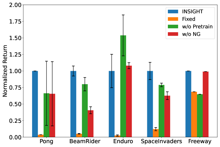
Figure 3: Performance of INSIGHT and its variants for five tasks. Refer to Fig. A1 for results for the remaining four tasks. Test returns are normalized so that INSIGHT corresponds to one and random policy is zero. Fixing the perception module during policy learning (i.e., Fixed) hinders performance for all tasks, indicating that it is crucial to refine states with reward signals. The results of w/o Pretrain and w/o NG show that pre-training the perception module and the proposed neural guidance scheme also contribute to the performance of INSIGHT.

4.2 Results

Task Performance  Tab. 1 shows that except for Pong, where visual observations are less involved, NS-RL baselines are outperformed by Neural by a wide margin. In contrast, INSIGHT can match or even outperform Neural. In addition, in Tab. A8 we show that our implementation for Neural matches the performance of CleanRL (Huang et al., 2022), an open-source implementation for deep RL agents. These results highlight that INSIGHT, by learning structured states and symbolic policies simultaneously, overcomes the performance drawback of existing NS-RL approaches. We now present an analysis for learning object coordinates and symbolic policies to explain the improvement.

Table 3: MAE and F-MAE for coordinate prediction. The lower, the better. F-MAE measures the mean absolute error of coordinate prediction for policy-related objects. Numbers are multiplied by 100. Refer to Tab. A7 for results for the other four tasks. By comparing the results of INSIGHT with those of Fixed, we see that refining state representations with rewards improves coordinate prediction for policy-related objects. The proposed neural guidance scheme is crucial for such improvement, as implied by results of w/o NG.

	INSIGHT		w/o Pretrain		Fixed		w/o NG		Coor-Neural
Tasks	MAE	F-MAE	MAE	F-MAE	MAE	F-MAE	MAE	F-MAE	MAE	F-MAE
Pong	$1.4\pm 0.9$	$\textbf{1.3}\pm 0.9$	$2.9\pm 3.1$	$3.5\pm 3.8$	$2.8\pm 0.5$	$3.1\pm 0.3$	$1.7\pm 0.9$	$1.6\pm 0.9$	$\textbf{0.9}\pm 0$	/
BeamRider	$\textbf{5.5}\pm 0$	$\textbf{3.2}\pm 0.3$	$5.8\pm 0.1$	$3.5\pm 0.1$	$\textbf{5.5}\pm 0.4$	$4.9\pm 0.1$	$6.2\pm 0.1$	$5.9\pm 0$	$5.7\pm 0$	/
Enduro	$13.5\pm 0$	$\textbf{6.7}\pm 0.3$	$13.1\pm 0.1$	$8.2\pm 0.2$	$\textbf{12.7}\pm 0.5$	$12.2\pm 0.5$	$13.4\pm 0.2$	$13.4\pm 0.2$	$13.7\pm 0.1$	/
SpaceInvaders	$10.3\pm 0.4$	$8.1\pm 0.9$	$10.6\pm 0.2$	$\textbf{6.5}\pm 0.6$	$\textbf{9.9}\pm 0.5$	$11.1\pm 0.4$	$11.1\pm 0.3$	$11.1\pm 0.4$	$10.3\pm 0.3$	/
Freeway	$16.3\pm 0.3$	$\textbf{14.8}\pm 1.6$	$23.4\pm 0$	$19.4\pm 5.6$	$\textbf{15.7}\pm 0.2$	$18.7\pm 0.8$	$16.4\pm 0.2$	$16.4\pm 0.2$	$16.4\pm 0.2$	/

Learning Object Coordinates  As mentioned in Sec. 3.1, the perception module of INSIGHT is more efficient than unsupervised tracking models such as SPACE. This argument is well supported by Tab. 2, which shows that both SPACE-Neural and SA-Neural are an order of magnitude slower than INSIGHT. In other words, for 10 million steps, the total inference time of SPACE-Neural exceeds 138 hours, whereas that of INSIGHT is less than six hours. In addition, we show in Tab. A5 that agents learn faster when learning object coordinates from the frame-symbol datasets. A possible reason is that the frame-symbol dataset provides direct supervision for object locations, while unsupervised methods are trained to reconstruct whole images and thus less focused on individual objects.

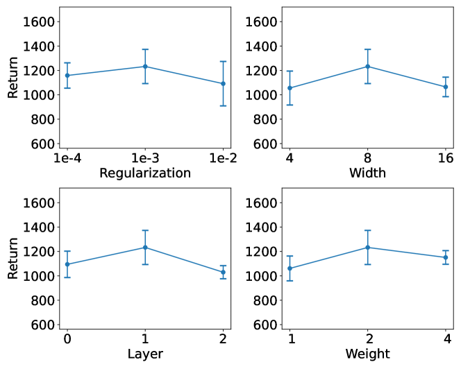
Figure 4: Influence of the weight for sparsity regularization $\lambda_{\text{reg}}$, the width/layer of the EQL actor, and the weight of $\mathcal{L}_{\text{cnn}}$ for SpaceInvaders. Results for other tasks are provided in Fig. A2. The performance of INSIGHT is quite robust against hyper-parameters.

Our main claim in this paper is that it is essential to refine structured states with both visual and reward information. We now examine this claim from the perspective of task performance and coordinate prediction. Fig. 3 shows that when compared to the variant Fixed, INSIGHT has significant better performance for all five task, demonstrating that INSIGHT’s performance is largely determined by its ability to refine structured states with reward signals. Tab. 3 further reveals a clue for the performance improvement. Compared to Fixed, INSIGHT has higher MAE for four tasks but lower F-MAE for all five tasks. In addition, readers may refer to Fig. A3 for visualizations of predicted coordinates. These findings suggest that reward signals can guide agents to improve the coordinate prediction of policy-relevant objects.

In Sec. 3.1, we suggest pre-training the perception module before policy learning. Fig. 3 shows that the pre-training step indeed improves performance for four tasks, and Tab. 3 indicates that the improvement may be the result of better prediction for policy-relevant objects. Meanwhile, this extra step does complicates the training protocol of INSIGHT. One possible improvement is to use off-policy algorithms for policy learning, which allow the perception module to be optimized for more gradient steps.

Learning Symbolic Policies  We introduce the neural guidance scheme to address the limited expressiveness of object coordinates. The effectiveness of this scheme is supported by results in Fig. 3–w/o NG performs worse than INSIGHT for three tasks out of five tasks. Moreover, Coor-Neural is outperformed by Neural for six tasks in Tab. 1, suggesting that the object coordinates are not sufficiently expressive for online policy learning. Tab. 3 reveals that unlike the case of INSIGHT, the F-MAE and MAE of w/o NG are almost the same, implying that w/o NG cannot improve coordinate prediction using reward signals. Thus, the neural guidance scheme plays a key role in improving performance by refining coordinate prediction with rewards.

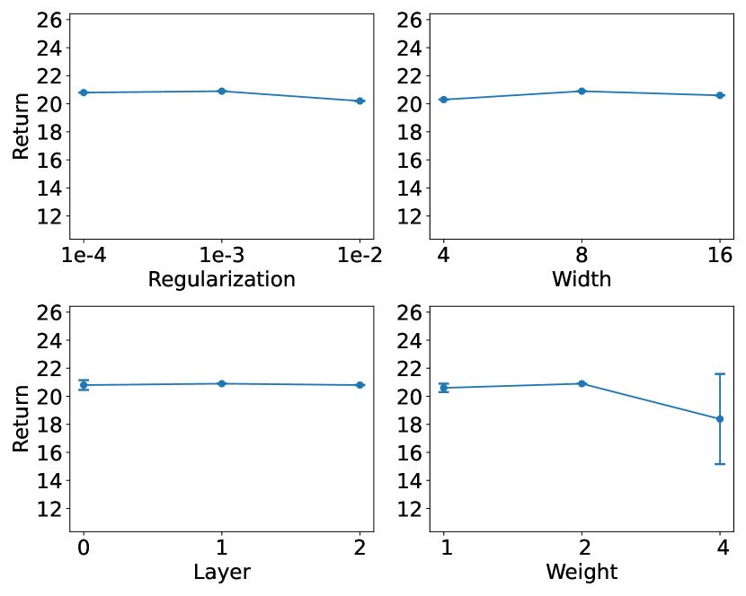
(a) Pong.

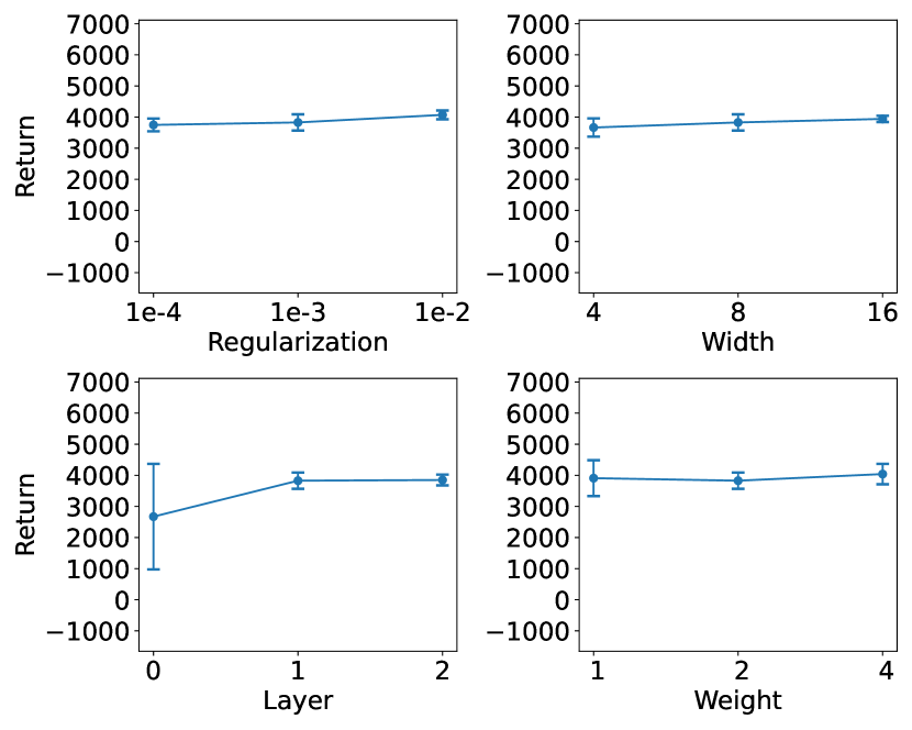
(b) BeamRider.

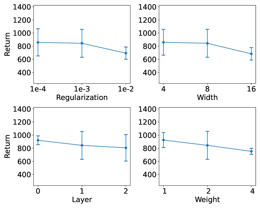
(c) Enduro.

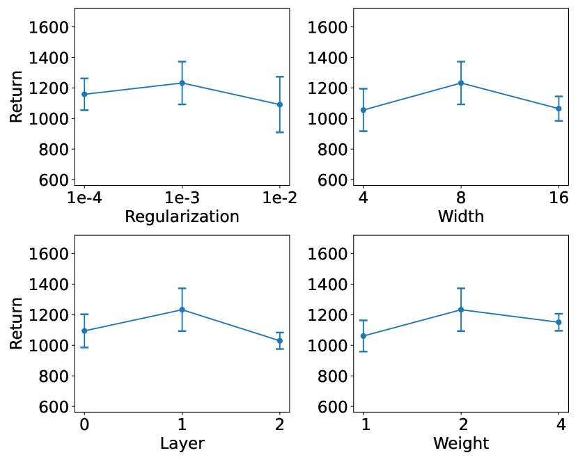
(d) SpaceInvaders.

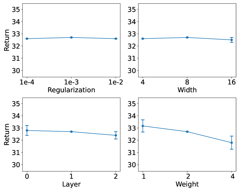
(e) FreeWay.

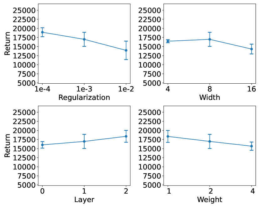
(f) Qbert.

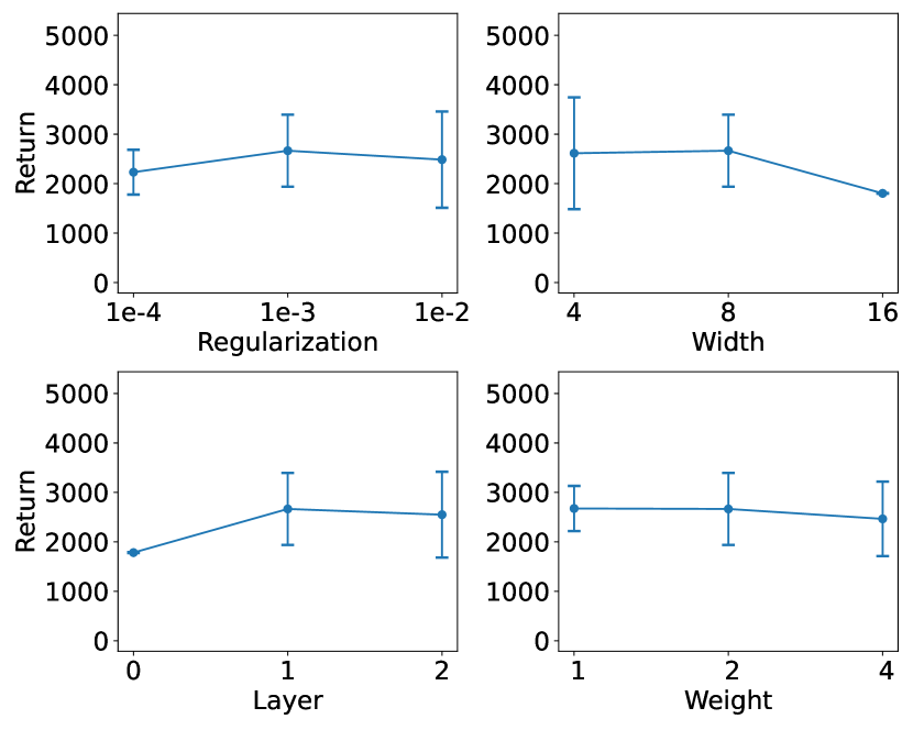
(g) Seaquest.

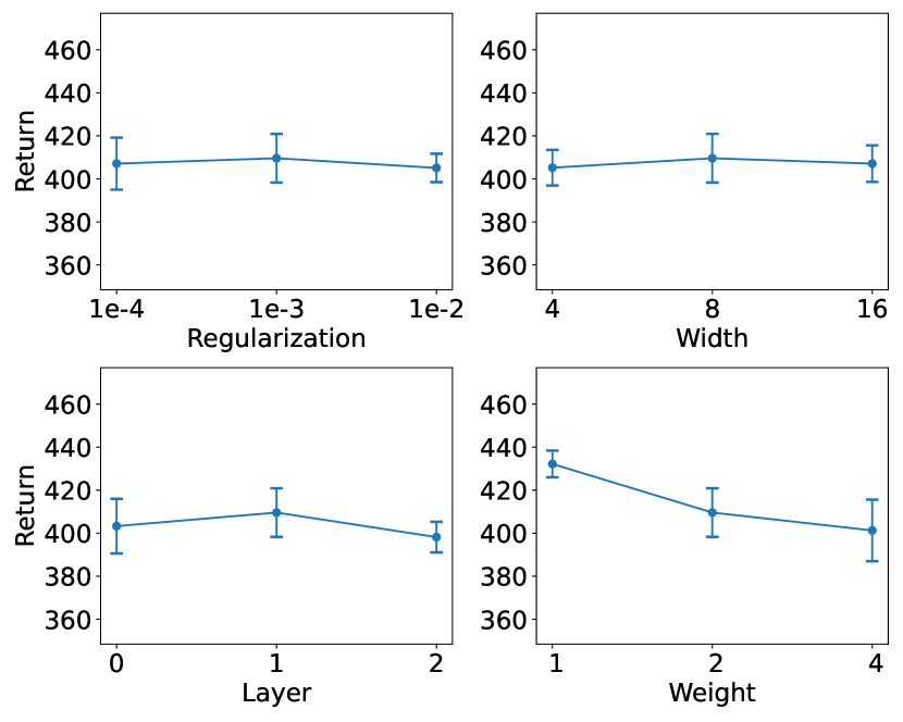
(h) Breakout.

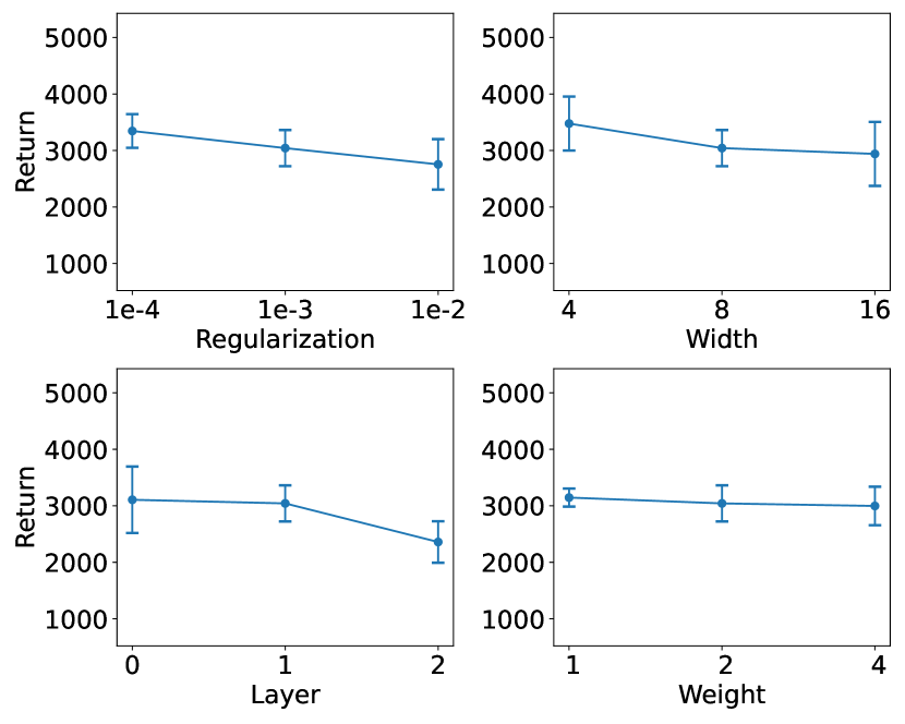
(i) MsPacman.

Figure A2: Effect of regularization coefficient $\lambda_{\text{reg}}$, the width of the EQL actor, the number of hidden layers in the EQL actor, and the weight of $\mathcal{L}_{\text{CNN}}$.

The Influence of Hyper-parameters  Finally, Fig. 4 shows the influence of four hyper-parameters for SpaceInvaders. Results for other tasks are provided in Fig. A2. It turns out that the performance of INSIGHT are quite robust against the hyper-parameters. Since our goal is to illustrate the efficacy of INSIGHT rather than benchmarking, we use the same values for hyper-parameters for all tasks.

In summary, the ability to refine states with reward signals is decisive for performance improvement, possibly due to the improved coordinate prediction for policy-relevant objects. The proposed neural guidance scheme also plays a role in improving task performance and coordinate prediction.

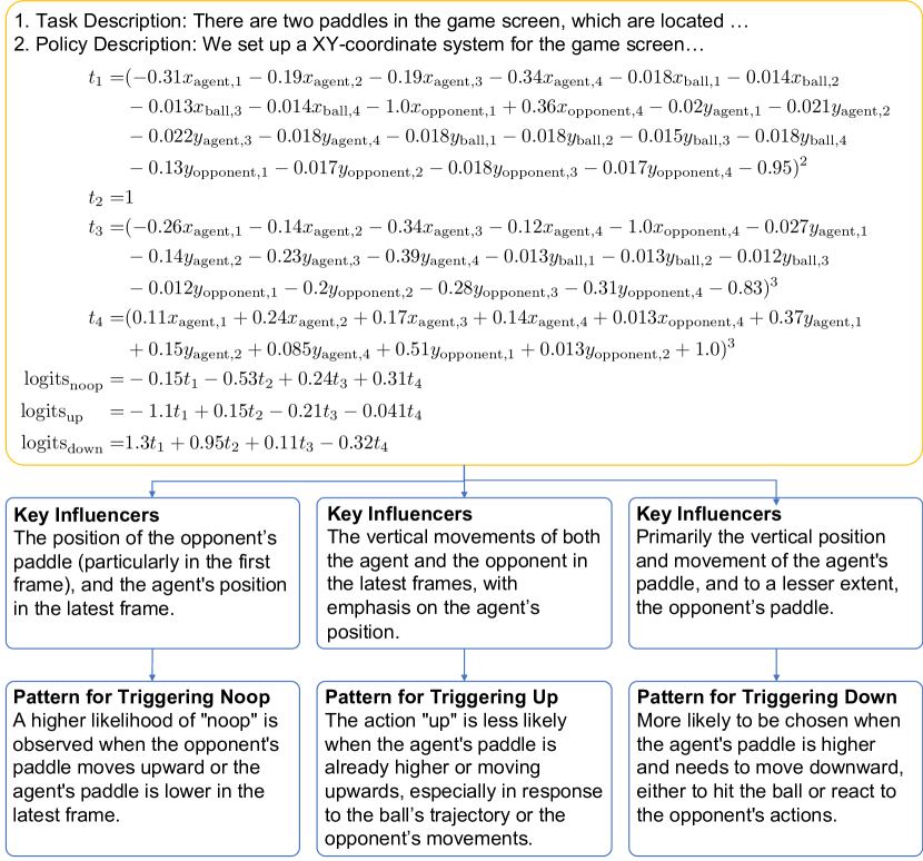
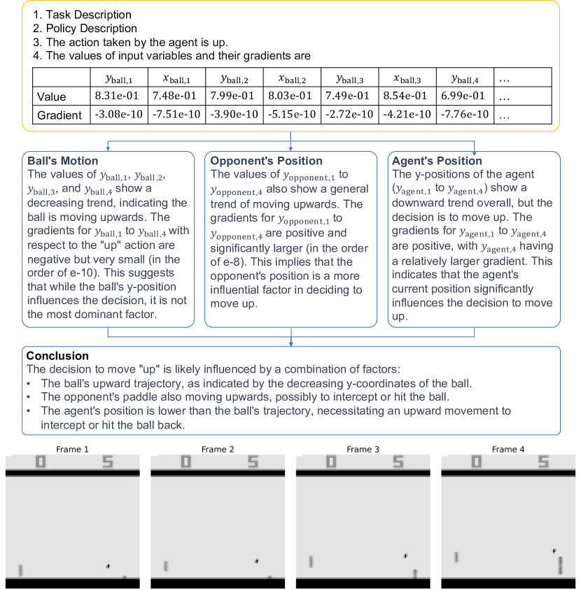
Figure 5: Examples for language explanations for Pong. Readers may refer to Appx. D for full prompts. Left: interpretations for a learned policy. The interpretations identify influential input variables and summarize triggering patterns of actions. Right: explanations for an action taken at a state. The four images located at the bottom illustrate the state. The motion of the ball and the opponent’s paddle are deduced from input variables, which are used for supporting explanations of actions.

4.3 Language Explanations

The left part of Fig. 5 presents interpretations of a policy learned for Pong. Readers may refer to the bottom right of Fig. 5 for screenshots of this game. Like a ping-pong game, an agent controls the right paddle to hit the ball to its opponent’s side and scores a point if the opponent fails to hit the ball back. Both paddles move only vertically.

The bottom left part of Fig. 5 shows policy interpretations generated by INSIGHT. It shows that the influential variables are correctly identified. For example, $y_{\text{opponent,1}}$ is recognized as influential for action noop due to its coefficient (-0.13), and the coordinates of the ball are omitted for their small coefficients. However, some triggering patterns are less convincing. Action up is considered to be less likely when the agent’s paddle moves upward ($y_{\text{agent}}$ decreases). While this is correct when considering $t_{3}$, it is in fact difficult to determine how $t_{1}$ changes in response to decrease of $y_{\text{agent}}$. These observations confirms the LLM’s ability to perform step-by-step analysis for symbolic policies.

The right part of Fig. 5 showcases decision explanations. The LLM correctly deduces the motion of the ball and the opponent’s paddle from the input coordinates, but it makes a mistake for the agent’s paddle, possibly due to fluctuations in the coordinate predictions. Moreover, by inspecting the gradients, it is pointed out that the decision is more sensitive to the position of the opponent’s paddle than the ball, suggesting that the agent is exploiting the opponent’s fixed policy. In the conclusion, the interpretations (e.g., to intercept or hit the ball) are supported by facts (e.g., the opponent’s motion), which can improve their credibility.

Overall, both the policy interpretation and the decision explanation are constructed from the information provided and are free of factual errors. They reveal some patterns in the agent’s decision-making process, although there are minor mistakes. Nevertheless, they suffice to explain the learned policies to users who are not familiar with NS-RL.

5 Conclusions

We propose INSIGHT, a framework that uses object coordinates as structured state representations and learns symbolic policies from visual input. INSIGHT is able to refine the structured states with reward signals by distilling vision foundation models into a scalable perception module, and it leverages a new neural guidance scheme to learn competitive symbolic policies from object coordinates, thereby overcoming the performance bottleneck of previous NS-RL approaches. Moreover, to improve model transparency for non-expert users, INSIGHT can generate language explanations for learned policies and specific decisions with LLMs. With experiments on nine Atari tasks, we show that INSIGHT outperforms all NS-RL baselines, and the improvement can be explained by the improved coordinate prediction for policy-relevant objects. We also showcase language explanations for learned policies and decisions.

Limitations

While the nine Atari tasks have already covered several critical issues, additional experiments for continuous control or realistic observation can complement our evaluation. Another limitation of INSIGHT is that EQL networks cannot express logical operations required by some reasoning tasks. Finally, quantitative evaluation of the explanations is also an interesting future topics.

Impact Statement

The goal of this paper is to improve the transparency of RL without sacrificing task performance, which paves the road towards trustworthy RL applications. From a societal point of view, we aim to reduce the barrier between general public and RL models, thus advancing the broad application of RL agents.

Appendix A Details of INSIGHT

A.1 Details of the Frame-Symbol Dataset

This section provides a detailed explanation of the frame-symbol dataset generation process, expanding on the preliminary overview presented in Sec. 3.1.

The generation of the dataset begins with a comprehensive training regimen of 10 million steps using the neural baseline. This regimen incorporates a neural policy tailored for interaction with the environment. During the final 1 million steps, specifically starting from the 9-millionth step, we capture a total of 10,000 frames, thereby forming an unsupervised frame dataset. This phase primarily focuses on documenting environmental interactions via image captures, with a special emphasis on acquiring objects in high-reward scenarios.

Following this, the initial frame undergoes processing through FastSAM, which identifies and segregates 256 unique objects by extracting their masks. These masks serve as inputs for the DeAot module, enabling object tracking across the subsequent 9,999 frames. FastSAM re-evaluates the scene every tenth frame to include new objects, leading to an increase in the object count. This increment prompts DeAot to start tracking these newly identified objects. For improved segmentation and tracking, all frames are resized to a resolution of 1024×1024 pixels.

During the segmentation phase using FastSAM, objects are excluded if their confidence level does not meet or exceed a threshold of 0.9. This stringent selection criterion is pivotal for minimizing misidentifications attributable to environmental factors. Moreover, within the same frame, a distinction is made between connected and non-connected masks. Connected masks that do not overlap with previously tracked objects are deemed new. Conversely, objects that overlap with an existing mask by 50% or less are also classified as new. The rationale for the former is to avoid fragmenting a single object into multiple smaller segments as much as possible, and for the latter, it is because the tracking module tends to recognize non-connected, similar objects as a single entity, necessitating their re-identification and enumeration.

In the dataset’s final development phase, the FastSAM module is deactivated, allowing DeAot to autonomously track objects from the initial to the final frame. The resulting dataset encompasses detailed information like object coordinates, bounding boxes, and RGB values, linked to their corresponding frames. Ultimately, this leads to the formation of a comprehensive frame-symbol dataset, where frames are stored at a resolution of 512×512 pixels. This process mitigates a previously identified limitation where the tracking model struggled to consistently detect objects in each frame. Conforming to the standard supervised training approach, the dataset is divided into training and test sets in an 80:20 ratio.

A.2 Label Weights of the Distribution-Balanced Focal Loss

Denote by $n_{j}={1}/{\sum_{i=1}^{N}c_{ij}}$ the inverse frequency of the $j$^th label, where $N$ is the number of samples in $\mathcal{D}_{\text{symbol}}$. The inverse frequency is further normalized, since the number of labels varies across samples, and transformed to the range $[\alpha,\alpha+1]$ for numerical stability. That is, the weight of label $c_{ij}$ is given by $\bar{\eta}_{ij}=\alpha+\sigma(\beta(\eta_{ij}-\mu))$, where $\eta_{ij}={n_{j}}/{\sum_{j^{\prime}}^{C}c_{ij^{\prime}}n_{j^{\prime}}}$ and $\sigma(\cdot)$ is the sigmoid function. $\alpha$, $\beta$, and $\mu$ are hyper-parameters.

A.3 Details of F-MAE

The F-MAE metric evaluates the precision of predicted object coordinates within frames of Atari tasks, with a focus on objects essential for the agent’s decision-making. Unlike traditional MAE, F-MAE targets a subset of objects identified as critical through symbolic regression. For a dataset $\mathcal{D}_{\text{symbol}}$ containing $N$ samples, the presence of the $j^{\text{th}}$ object in the $i^{\text{th}}$ sample is marked by $c_{ij}$, where $c_{ij}=1$ indicates the object’s presence, and $c_{ij}=0$ its absence. Let $\mathbf{x}_{i}\in\mathbb{R}^{2C}$ represent the vector of object coordinates in the $i^{\text{th}}$ image, and $\mathbf{\hat{x}}_{i}$ its predicted counterpart. For objects numbered $j=1,2,\dots,C$, the coordinates $x_{i,2j}$ and $x_{i,2j+1}$ correspond to the Y and X positions, respectively. The F-MAE, focusing on a critical subset of objects denoted as $S$, is calculated using Eq. A1:

$$\text{F-MAE}= \frac{1}{2EN|S|}\sum_{i=1}^{N}\sum_{j=1}^{C}s_{ij}c_{ij}\left(\left|x_{i,2j}-\hat{x}_{i,2j}\right|+\left|x_{i,2j+1}-\hat{x}_{i,2j+1}\right|\right).$$ (A1)

Here, $s_{ij}$ denotes the inclusion of the $j^{\text{th}}$ object in the $i^{\text{th}}$ sample within the filtered subset, taking a value of 1 when included and 0 otherwise. The term $E$ represents the total number of frames featuring the objects after filtering. The division by 2 accounts for the mean impact of the x and y coordinates. The term $|S|$ signifies the count of objects post-filtering, with the division by $|S|$ adjusting for the impact of individual objects. This formula constrains the F-MAE’s range between 0 and 1, where 0 indicates perfect accuracy and 1 denotes complete inaccuracy, thus providing a clear metric for evaluating object coordinate prediction precision within task frames.

A.4 Conditions for Testing Inference Speed

In the experiments conducted as detailed in Tab. 2, the hardware setup comprised an AMD Ryzen 9 5950X 16-Core Processor for CPU, an NVIDIA GeForce RTX 3090 Ti as the graphics card, and 24564MiB of video memory. Each experiment involved executing 1000 steps on the Pong task, from which the average single-step inference time of the model was calculated.

Appendix B Experimental Setup

B.1 Architecture and Hyperparameters

CNN Encoder Structure

In Tab. A1, the structure of the CNN encoder is elaborated. Comprising three convolutional layers, each layer is distinctively configured with varying kernel sizes, strides, padding, and channel outputs. The initial resolution of the image is defined as 84x84 pixels, encompassing four channels. These channels amalgamate the grayscale images from the previous four temporal frames, capturing motion information.

Table A1: Hyperparameters of the CNN Encoder

Hyperparameter	Value
Resolution	84x84
Image Channels	4
Encoder Configuration
Layer	Kernel Size	Stride	Padding	Channels	Activation
Conv1	5x5	2	2	32	ReLU
Conv2	5x5	2	2	64	ReLU
Conv3	5x5	1	2	64	ReLU
Post-Convolution Layers
Layer	Out Feature	Activation
Flatten	-	-
Linear	2048	ReLU
LayerNorm	2048	-
Output Layers
Layer	Structure	Activation
Existence Layer	Linear(2048, 1024)	ReLU
	Linear(1024, 1024)	-
Coordinate Layer	Linear(2048, 2048)	ReLU
	Linear(2048, 2048)	-
Shape Layer	Linear(2048, 512)	ReLU
	Linear(512, 512)	-

The initial convolutional layer (Conv1) utilizes a 5x5 kernel, a stride of 2, and padding of 2 to output 32 channels. This configuration begins the feature extraction process, reducing spatial dimensions while enriching the feature map’s depth. The following layers (Conv2 and Conv3) maintain this configuration but with an increased channel output of 64, capturing more intricate features.

Post-convolution, the network integrates a flattening step, converting the multi-dimensional feature maps into a singular vector. This vector feeds into a fully connected linear layer with 2048 output features and ReLU activation, transforming the detailed convolutional features for subsequent analysis.

A layer normalization follows the first linear layer, enhancing the learning process’s stability and efficiency. This normalization standardizes data scales and enables faster training through higher learning rates.

In the final stage, the network includes distinct output layers for existence, coordinate, and shape predictions. The Existence Layer initially compresses the feature dimensions from 2048 to 1024 using a ReLU activation function. This is succeeded by a subsequent linear layer, which maintains this reduced feature dimension. The Coordinate Layer, conversely, preserves the feature count at 2048, while the Shape Layer diminishes it to 512. Both these layers incorporate ReLU activations and are followed by linear transformations for processing.

EQL Structure

The input dimension of the EQL network is configured as 2048, specifically designed to accommodate the coordinate representation generated by the encoder. These coordinates are initially processed through a hidden layer, followed by a custom activation function. The activation function employs a variety of operations to avoid excessive gradient explosion and ensure sufficient representation ability. These include squaring ($f(x)=x^{2}$), cubing ($f(x)=x^{3}$), constant ($f(x)=c$), identity ($f(x)=x$), product ($f(x,y)=xy$), and addition ($f(x,y)=x+y$). Each of these functions is iteratively applied four times within the hidden layer, as detailed in Tab. A2. Subsequently, the output layer generates a symbolic expression corresponding to each action dimension within the environment. This process includes a transition through a softmax layer, where the final action is derived by random sampling from the resulting probability distribution. Furthermore, the output of the EQL network is multiplied by a temperature coefficient $t_{eql}=10$, enhancing sensitivity to coordinate changes and aiding in the preservation of object coordinate prediction during policy learning.

Table A2: Hyperparameters of EQL Network

Hyperparameter	Value
Input Dimensions	2048
Activation Function 1	$f(x)=x^{2}$
Activation Function 2	$f(x)=x^{3}$
Activation Function 3	$f(x)=c$
Activation Function 4	$f(x)=x$
Activation Function 5	$f(x,y)=xy$
Activation Function 6	$f(x,y)=x+y$
Number of Repetitions	4
Number of Hidden Layers	1
$t_{eql}$	10

Table A3: Hyperparameter of Pretraining

Hyperparameter	Value
Epoch	600
Batch Size	32
Learning Rate	$3\times 10^{-4}$
Weight Decay	$1\times 10^{-4}$
$\alpha$ of $\mathcal{L}_{\text{exist}}$	0.1
$\beta$ of $\mathcal{L}_{\text{exist}}$	10
$\mu$ of $\mathcal{L}_{\text{exist}}$	Mean Value of $n_{j}$
$\gamma$ of $\mathcal{L}_{\text{exist}}$	2
Optimizer	Adam
Loss Function	Eq. 3

Table A4: Hyperparameters of Policy Learning

Hyperparameter	Value
Total Steps	10M
Learning Rate	$2.5\times 10^{-4}$
Batch Size	1024
Initial value of $\lambda_{\text{reg}}$	$1\times 10^{-3}$
Coefficient for annealing $\lambda_{\text{reg}}$ linearly	$\frac{\text{Update}-1}{\text{Total Updates}}$
$\lambda_{\text{cnn}}$	2

Pretraining

The pretraining stage employed the loss function detailed in Eq. 3, spanning 600 epochs with a batch size of 32. To counteract overfitting, a weight decay regularization of $1\times 10^{-4}$ was applied. The learning rate was established at $3\times 10^{-4}$, with the Adam optimizer selected for its effectiveness in gradient descent optimization. Detailed specifics of the parameters, including their command line arguments and values, are provided in Tab. A3.

Policy Learing

In the policy learning phase, following the common settings of Atari tasks, INSIGHT interacts with the environment for 10M steps. PPO with a learning rate of 2.5e-4 uses the collected rewards to optimize the model. The batchsize size of each update is 1024. In order to ensure that the network can learn useful policies while ensuring the coefficient of the policy, we choose to use 1e-3 regularization and increase the regularization coefficient from 0 to 1 in each update. In addition, we multiply the coefficient of Eq. 3 by 2 to enhance the accuracy of coordinate prediction. All detailed parameters are summarized in Tab. A4.

Appendix C Additional Experimental Results

This section encompasses all supplementary experiments, providing a comprehensive overview.

C.1 Comprehensive Evaluation of Representations

We highlight an additional advantage of adopting a distilled vision-based model: enhanced efficiency in task learning through improved representations. Tab. A5 presents the task performance of different approach to extract state representations accompanied by neural actors.

Table A5: Performance of SA-Neural, SPACE-Neural, Coor-Neural, and Neural when trained for one million steps. Coor-Neural outperforms SA-Neural and SPACE-Neural on most tasks and is the only method that can compete with Neural, which shows that agents learn faster when using our proposed method of learning structured state representations.

Tasks	SA-Neural	SPACE-Neural	Coor-Neural	Neural
Pong	$5.4\pm 0.5$	$-20.6\pm 0$	$10.4\pm 6.2$	$\textbf{16.8}\pm 3.8$
BeamRider	$684.8\pm 587.1$	$579.6\pm 348.4$	$\textbf{846.1}\pm 92.2$	$551.6\pm 25.1$
Enduro	$0\pm 0$	$8.1\pm 8.4$	$\textbf{45.4}\pm 63.5$	$9.7\pm 6.9$
SpaceInvaders	$35.8\pm 58.2$	$135\pm 134.4$	$\textbf{492.5}\pm 61.4$	$490.4\pm 32.3$
Freeway	$0\pm 0$	$0\pm 0$	$\textbf{27.8}\pm 2.9$	$17.1\pm 12.9$
Qbert	$1085.2\pm 0.5$	$289.1\pm 0$	$2030.2\pm 383.9$	$\textbf{5659.2}\pm 1271.5$
Seaquest	$955.2\pm 587.1$	$200.3\pm 348.4$	$718.1\pm 112.1$	$\textbf{1297.3}\pm 359.6$
Breakout	$\textbf{65.5}\pm 0$	$1\pm 8.4$	$39.7\pm 4.2$	$34.7\pm 23.5$
MsPacman	$643.2\pm 58.2$	$60.4\pm 134.4$	$1180.2\pm 245.9$	$\textbf{1289.2}\pm 106.7$

Table A6: Performance of SA-Neural, SPACE-Neural, Coor-Neural, and Neural when trained for three million steps. Coor-Neural consistently achieves higher performance than SA-Neural and SPACE-Neural in the case of convergence.

Tasks	SA-Neural	SPACE-Neural	Coor-Neural	Neural
Pong	$17.2\pm 3$	$-20.6\pm 0$	$19.7\pm 0$	$\textbf{19.9}\pm 0.3$
Freeway	$19.8\pm 15$	$12.2\pm 3$	$\textbf{31.6}\pm 0.1$	$25.3\pm 6.8$

These methods were trained for only one million steps due to the poor efficiency of SPACE-Neural. Similar experiment setup has been utilized by Delfosse et al. (2023b). We also report results for three million steps in Tab. A6, by which point the performances on Pong and Freeway had stabilized. Note that compared to slot attention or the SPACE model, our perception module leads to better performance. This is because our image-symbol dataset provides direct supervision for the location of objects. On the contrary, unsupervised methods are trained to reconstruct whole images and thus less focused on individual objects.

C.2 Analysis of Coordinate Accuracy

Tab. 3 presents a quantitative assessment of the coordinate prediction accuracy achieved by our method. In Tab. A7, we document the experimental results for the additional four tasks. Notably, the F-MAE on Qbert, Seaquest, and MsPacman post-training markedly surpasses the pre-training figures. This improvement suggests that end-to-end fine-tuning significantly enhances the strategic relevance of object coordinate accuracy.

Table A7: MAE and F-MAE for coordinate prediction for Qbert, Seaquest, Breakout and MsPacman. Numbers are multiplied by 100.

	INSIGHT		w/o Pretrain		Fix		w/o NG		Coor-Neural
Tasks	MAE	F-MAE	MAE	F-MAE	MAE	F-MAE	MAE	F-MAE	MAE	F-MAE
Qbert	$1.3\pm 0$	$\textbf{0.8}\pm 0$	$1.4\pm 0.1$	$0.9\pm 0.1$	$\textbf{1}\pm 0$	$0.9\pm 0.1$	$1.4\pm 0.1$	$1.4\pm 0.1$	$1.7\pm 0.1$	/
Seaquest	$4.2\pm 0.1$	$\textbf{1.9}\pm 0.2$	$4.5\pm 0.1$	$2\pm 0.2$	$\textbf{4.1}\pm 0.1$	$3.7\pm 0.3$	$4.4\pm 0.1$	$4.4\pm 0.1$	$4.5\pm 0.1$	/
Breakout	$7.3\pm 0.4$	$5.4\pm 0.6$	$6.4\pm 0.1$	$4.2\pm 0.3$	$\textbf{4.5}\pm 0.2$	$\textbf{2.5}\pm 0.1$	$5.2\pm 0.3$	$5.2\pm 0.3$	$6.7\pm 0.7$	/
MsPacman	$7.2\pm 0.1$	$\textbf{4.3}\pm 0.5$	$6.9\pm 0.2$	$5.1\pm 0.4$	$\textbf{6.5}\pm 0.2$	$6.8\pm 0.7$	$7.2\pm 0.3$	$7.2\pm 0.3$	$6.9\pm 0.3$	/

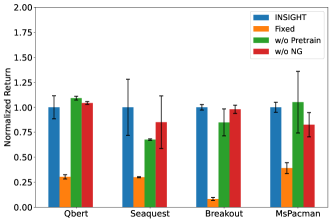
Figure A1: Performance of INSIGHT and it variants for Qbert, Seaquest, Breakout and MsPacman.

C.3 Extended Ablation Study Details

This subsection extends the ablation studies detailed in Fig. 3 and Fig. 4 to encompass all tasks, as referenced in Fig. A1-Fig. 2(i). Notably, the comprehensive ablation analysis presented in Fig. A1 demonstrates performance declines in most tasks when methods are modified. Furthermore, the consistency observed across various hyperparameters, as shown in Fig. 2(a)-Fig. 2(i), corroborates the findings discussed in Sec. 4.2.

Table A8: Performance of the proposed INSIGHT, Neural and CleanRL (Huang et al., 2022)) on nine Atari tasks. INSIGHT matches the performance of Neural for all nine tasks and outperforms all NS-RL baselines. Our neural baseline is contestable for the CleanRL baseline in most cases.

Task	INSIGHT	Neural	CleanRL
Pong	$\textbf{20.9}\pm 0.1$	$20.4\pm 0.6$	$20.7\pm 0.4$
BeamRider	$3828.1\pm 261.1$	$\textbf{3868.1}\pm 204.2$	$2270.5\pm 107.3$
Enduro	$843.7\pm 213.8$	$676.9\pm 730.4$	$\textbf{1006.6}\pm 244.1$
Qbert	$16978.6\pm 1936.1$	$\textbf{17879.2}\pm 1857.1$	$16619.8\pm 256.3$
SpaceInvaders	$\textbf{1232.6}\pm 140.7$	$1184.6\pm 137.6$	$1023.1\pm 160.2$
Seaquest	$\textbf{2665.7}\pm 728.2$	$1804.8\pm 20.1$	$1841.2\pm 17.1$
Breakout	$\textbf{409.6}\pm 11.3$	$259.6\pm 183.8$	$387.8\pm 11.8$
Freeway	$\textbf{32.7}\pm 0.1$	$28.7\pm 5.3$	$32.2\pm 1.1$
MsPacman	$\textbf{3042.5}\pm 320.1$	$2737.1\pm 562.3$	$2237.2\pm 163.5$

(a) Pong (before).

(b) Pong (after).

(c) BeamRider (before).

(d) BeamRider (after).

(e) Enduro (before).

(f) Enduro (after).

(g) Seaquest (before).

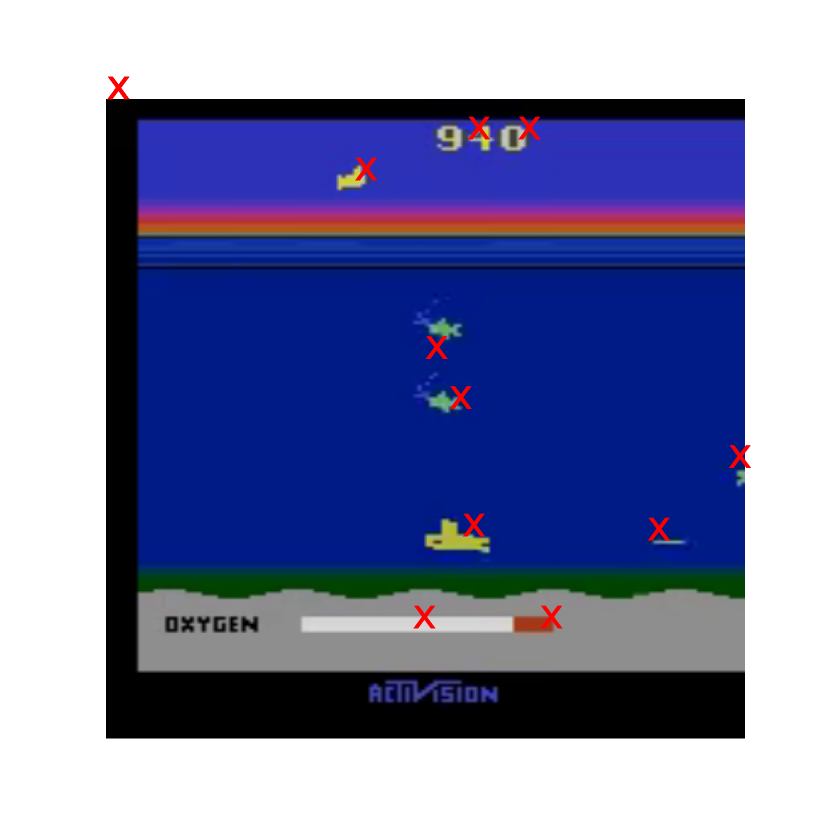
(h) Seaquest (after).

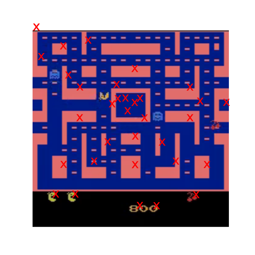
(i) MsPacman (before).

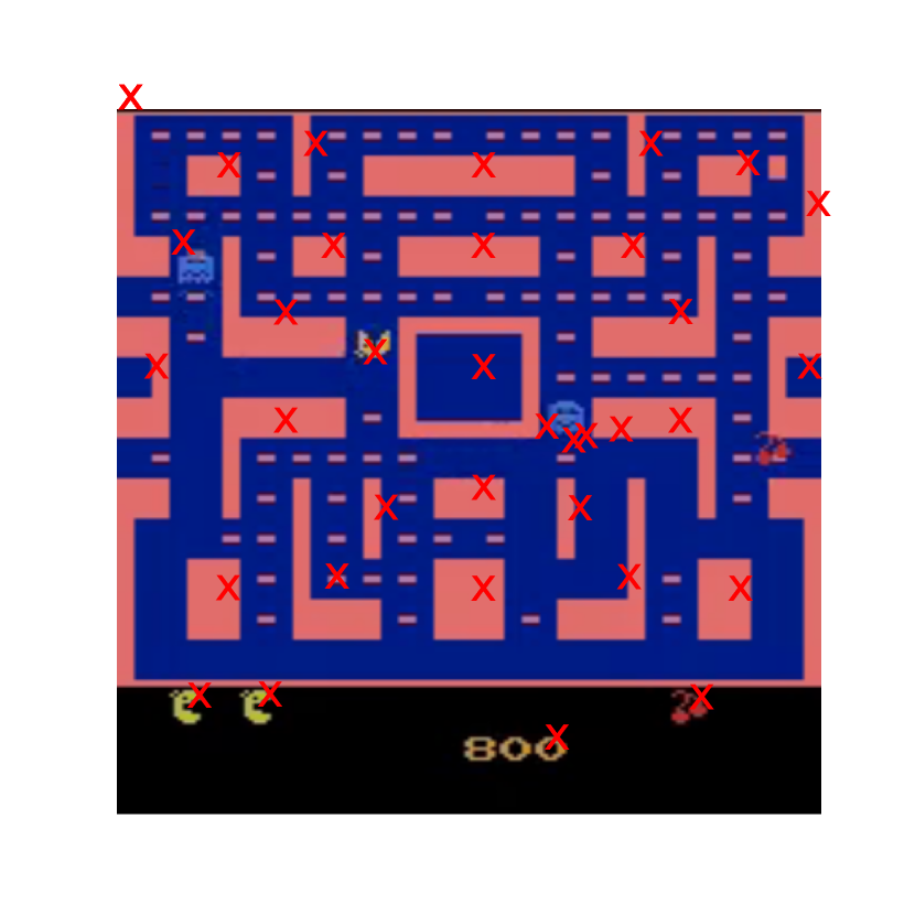
(j) MsPacman (after).

Figure A3: Predicted coordinates before and after policy learning.

C.4 Additional Baseline

In this section, we introduce an additional baseline, CleanRL, to evaluate the performance of INSIGHT. CleanRL is an open-source implementation derived from the CleanRL library (Huang et al., 2022). The sole modification involves adjusting the CNN’s output dimension from 512 to 2048 or higher to facilitate a fair comparison with our framework. It is noteworthy that our neural baseline exhibits competitive performance relative to CleanRL. As shown in Tab. A8, INSIGHT achieves superior returns in six tasks, unequivocally demonstrating its capability to outperform existing neural policies in online environments.

C.5 Visualized Coordinate Tracking

In this section, we expand upon the advantages of end-to-end training for coordinate prediction, initially presented in Tab. 3, by offering a more intuitive visualization. Fig. A3 illustrates the object coordinates before and after the training process. For instance, in Figs. 3(b) and 3(a), we note a marked reduction in the pixel coordinate shift of the ball post-training. Similarly, the laser emitted by the agent in Figs. 3(d) and 3(c) and the car on the road in Figs. 3(f) and 3(e) exhibit significantly diminished pixel coordinate shifts following training. Moreover, post-training observations in Figs. 3(h) and 3(g) reveal the successful detection of enemy coordinates at the periphery, a detail that was previously unattainable. Lastly, in Figs. 3(j) and 3(i), the model demonstrates its ability to consistently track the blue enemy post-training, overcoming the initial limitation of losing track of the object.

Appendix D Comprehensive Prompt Template Overview

In this section, the full prompt template is presented. It comprises a public description template, along with two distinct policy illustration templates. The public description template outlines the fundamental aspects of the task and the underlying policy (refer to Tab. A9 and Tab. A10). The policy illustration templates are further bifurcated into policy explanation and decision explanation, detailed in Tab. A11 and Tab. A12, respectively.

Table A9: The first part of pong’s public prompt.

You need to help a user to analyze a control policy for the task Pong available in the OpenAI Gym repository. The policy is obtained with deep reinforcement learning.

You need to first understand the goal of the task and the policy.

# task Description

There are two paddles in the task screen, which are located at the left and right side of the screen. The agent controls the right paddle, and its opponent controls the left paddle. Both of them can only control the paddle to move up or down. They cannot move leftward or rightward

Like a pingpong task, the agent competes against its opponent by stricking the ball to the opponent’s side (left). The agent earns a point if its opponent fails to strick the ball back.

The agent needs to solve the task in discrete steps. At each step, it takes as input the task screen, and it needs to take one of the three actions:

noop: take no operation

up: move its paddle upward.

down: move its paddle downward.

# The policy

## Input Variable

We set up a xOy-coordinate system for the task screen. The origin is at the upper left corner. The positive direction of the y-axis is downwards, and the positive direction of the x-axis is to the right. We provide the agent with the latest four consecutive frames and use the coordinates of objects in these frames as input. Frame 4 is the current frame. Frame 3 is the frame obtained at one step before. Frame 2 is the frame obtained at two steps before, and frame 1 is the frame obtained at three steps before. You can use the coordinates of the same object in different time steps to infer the motion of the object.

The objects of interest are the agent, the opponent, and the ball. The input variables follows this naming convention: [x/y]_object_frame. For example, x_agent_1 is the x coordinate of the agent at frame 1. Remember, the input variables represent coordinates of some objects, and they are in the range [0,1].

Table A10: The second part of pong’s public prompt.

## Logits

logits_noop1 = -0.56*y_agent_1**2 - 0.38*y_agent_1*y_agent_2 - 0.087*y_agent_1*y_opponent_1 - 0.16*y_agent_1*y_opponent_2 - 0.76*y_agent_1*y_opponent_3 - 0.51*y_agent_1*y_opponent_4 - 0.54*y_agent_1 - 0.24*y_agent_2**2 - 0.073*y_agent_2 + 0.27*y_agent_4**2 + 0.55*y_agent_4 - 0.078*y_opponent_1**2 - 0.33*y_opponent_1*y_opponent_2 - 0.2*y_opponent_1 - 0.35*y_opponent_2**2 - 0.5*y_opponent_2 - 0.34*y_opponent_3**2 - 0.45*y_opponent_3*y_opponent_4 - 0.32*y_opponent_3 - 0.15*y_opponent_4**2 - 0.19*y_opponent_4 + 1.1

logits_noop2 = -0.074*y_agent_1*y_opponent_2 + 0.059*y_agent_1*y_opponent_3 - 0.097*y_agent_4 - 0.16*y_opponent_1*y_opponent_2 - 0.18*y_opponent_2**2 - 0.27*y_opponent_2 + 0.063*y_opponent_4

logits_up1 = 0.23*y_agent_1**2 + 0.59*y_agent_1*y_agent_2 + 0.4*y_agent_2**2 + 0.11*y_agent_2 - 1.5*y_agent_4**2 - 3.6*y_agent_4 + 0.068*y_opponent_3 + 1.1

logits_down1 = 0.09*x_ball_3 + 0.12*x_ball_4 - 0.21*y_agent_1**2 + 0.12*y_agent_1*y_opponent_1 + 0.27*y_agent_1*y_opponent_2 - 0.43*y_agent_1*y_opponent_3 - 0.28*y_agent_1*y_opponent_4 + 0.13*y_agent_2 + 0.14*y_agent_4**2 + 0.43*y_agent_4 + 0.087*y_ball_3 + 0.15*y_ball_4 + 0.14*y_opponent_1**2 + 0.6*y_opponent_1*y_opponent_2 + 0.61*y_opponent_1 + 0.65*y_opponent_2**2 + 1.1*y_opponent_2 - 0.2*y_opponent_3**2 - 0.26*y_opponent_3*y_opponent_4 - 2.8*y_opponent_3 - 0.085*y_opponent_4**2 - 0.14*y_opponent_4 - 2.3

logits_up2 = 0.063*x_ball_4 - 0.078*y_agent_1 + 0.18*y_agent_2**2 + 0.52*y_agent_2*y_agent_3 + 0.35*y_agent_2*y_opponent_1 + 0.29*y_agent_2*y_opponent_2 + 0.26*y_agent_2 + 0.38*y_agent_3**2 + 0.51*y_agent_3*y_opponent_1 + 0.42*y_agent_3*y_opponent_2 + 1.6*y_agent_3 - 8.2*y_agent_4 - 0.085*y_ball_3 + 0.17*y_opponent_1**2 + 0.28*y_opponent_1*y_opponent_2 + 0.45*y_opponent_1 + 0.11*y_opponent_2**2 + 0.15*y_opponent_2 - 0.074*y_opponent_3 + 0.26

logits_down2 = -0.052*x_ball_1 - 0.068*x_ball_3 - 0.093*x_ball_4 + 0.18*y_agent_1 - 0.17*y_agent_2**2 - 0.49*y_agent_2*y_agent_3 - 0.33*y_agent_2*y_opponent_1 - 0.27*y_agent_2*y_opponent_2 - 0.39*y_agent_2 - 0.35*y_agent_3**2 - 0.48*y_agent_3*y_opponent_1 - 0.4*y_agent_3*y_opponent_2 - 0.38*y_agent_3 + 0.15*y_agent_4**2 + 0.54*y_agent_4 - 0.06*y_ball_1 - 0.064*y_ball_3 - 0.11*y_ball_4 - 0.17*y_opponent_1**2 - 0.28*y_opponent_1*y_opponent_2 - 0.58*y_opponent_1 - 0.13*y_opponent_2**2 - 0.38*y_opponent_2 + 2.2*y_opponent_3 - 0.052*y_opponent_4 - 3.6

## The Probability of Actions

action_noop = [exp(logits_noop1) + exp(logits_noop2)] / sum(exp(logits))

action_up = [exp(logits_up1) + exp(logits_up2)] / sum(exp(logits))

action_down = [exp(logits_down1) + exp(logits_down2)] / sum(exp(logits))

Table A11: Pong’s policy interpretation prompt.

# Your Task

You need to analyze this policy based on its mathematical properties. You must follow the following rules.

1. You can also leverage your own knowledge about the goal of the task, but the conclusions for the policies have to be based on the mathematical properties of the policy.

2. You need to analyze the policy in these three steps: (a) analyze how changes in variables affect action logits, (b) analyze how changes in logits affect the probability of taking action, and (c) summarize the Influence of input variables on action probabilities.

3. When performing (a), remember that the input variables represent the location of an object. Take into consideration that the input variables are within [0,1]. Pay attention to the coefficients of each input variable and constants (if any).

4. When performing (b), remember that the probability of actions sum to one.

5. An increase of the logit of certain actions might results in an increase in the probability of that action. A decrease of the logit of certain actions might results in an decrease in the probability of that action.

6. When performing (c), summarize your findings from (a) and (b).

For example, for logits_up1, first think about the coefficient of x_ball_2. Since the values of x_ball_2 are within [0,1], how does it affect the logit of moving up? How does it affect the probability of moving up?

7. Be specific the effect of each term.

## Output

Organize your response as (1) equation, (2) influential variables, and (3) analysis. Render the equations into latex format. Use the object names and frame indices as subscripts. For example, y_\text{agent,1}. Use the name of actions as the subscript of logits. For example, logits_\text{noop}. Only keep two significant digits for each number.

Now, analyze action noop.

{Chatgpt response}

Analyze action up.

{Chatgpt response}

Analyze action down.

Provide a summary for your recent analysis. Follow the rules below.

1. Be specific on when will the agent chooses certain actions.

2. Your summary should be consistent with your analysis.

3. Organize your response in markdown format.

Here is a recap for our set up.

{Recap in public prompt}

Table A12: Pong’s decision explanation prompt.

# Your Task

We used this policy to play the task and collected some data. You need to explain why the agent took a specific action when the input variables took specific values.

The action taken by the agent is up.

The value of y_ball_1 is 0.9018810391426086

The gradient of the log-likelihood for action up with respect to y_ball_1 is 2.75e-04.

The value of x_ball_1 is 0.5703107714653015

The gradient of the log-likelihood for action up with respect to x_ball_1 is -4.13e-04.

The value of y_ball_2 is 0.5564423203468323

The gradient of the log-likelihood for action up with respect to y_ball_2 is -4.36e-04.

The value of x_ball_2 is 0.6364298462867737

The gradient of the log-likelihood for action up with respect to x_ball_2 is -7.43e-06.

The value of y_ball_3 is 0.4664875864982605

The gradient of the log-likelihood for action up with respect to y_ball_3 is -8.24e-04.

The value of x_ball_3 is 0.7508251070976257

The gradient of the log-likelihood for action up with respect to x_ball_3 is 3.87e-04.

The value of y_ball_4 is 0.7325012683868408

The gradient of the log-likelihood for action up with respect to y_ball_4 is 7.06e-04.

The value of x_ball_4 is 1.0

The gradient of the log-likelihood for action up with respect to x_ball_4 is 1.34e-03.

The value of y_opponent_1 is 1.0

The gradient of the log-likelihood for action up with respect to y_opponent_1 is 2.09e-02.

The value of y_opponent_2 is 1.0

The gradient of the log-likelihood for action up with respect to y_opponent_2 is 1.67e-02.

The value of y_opponent_3 is 1.0

The gradient of the log-likelihood for action up with respect to y_opponent_3 is -2.63e-03.

The value of y_opponent_4 is 1.0

The gradient of the log-likelihood for action up with respect to y_opponent_4 is -8.92e-04.

The value of y_agent_1 is 1.0

The gradient of the log-likelihood for action up with respect to y_agent_1 is -1.39e-02.

The value of y_agent_2 is 1.0

The gradient of the log-likelihood for action up with respect to y_agent_2 is 4.85e-03.

The value of y_agent_3 is 1.0

The gradient of the log-likelihood for action up with respect to y_agent_3 is 4.58e-02.

The value of y_agent_4 is 0.0

The gradient of the log-likelihood for action up with respect to y_agent_4 is -4.94e-02.

## Output

You need to provide a concise explanation for why the agent took this action when the input variables took these values.

For example, would the agent earn a point by choosing such an action?

There are a few rules that need to be followed.

1. Your explanations should be specific. You should explain why the action up is preferred over other actions.

2. Your explanations should be easy to read.

3. Your explanations should be entirely based on the equations for the policy, the values of input variables, and the gradients of action log-likelihood with respect to input variables.

4. Your explanations should be consistent with the definition of the input variables and the coordinate system.

Render the equations into latex format. Use the object names and frame indices as subscripts. For example, y_\text{agent,1}. Use the name of actions as the subscript of logits. For example, logits_\text{noop}. Only keep two significant digits for each number.

References

- Agarwal et al. (2021) Agarwal, R., Schwarzer, M., Castro, P. S., Courville, A. C., and Bellemare, M. Deep reinforcement learning at the edge of the statistical precipice. Advances in neural information processing systems, 34:29304–29320, 2021.
- Bills et al. (2023) Bills, S., Cammarata, N., Mossing, D., Tillman, H., Gao, L., Goh, G., Sutskever, I., Leike, J., Wu, J., and Saunders, W. Language models can explain neurons in language models. URL https://openaipublic. blob. core. windows. net/neuron-explainer/paper/index. html.(Date accessed: 14.05. 2023), 2023.
- Bubeck et al. (2023) Bubeck, S., Chandrasekaran, V., Eldan, R., Gehrke, J., Horvitz, E., Kamar, E., Lee, P., Lee, Y. T., Li, Y., Lundberg, S., et al. Sparks of artificial general intelligence: Early experiments with gpt-4. arXiv preprint arXiv:2303.12712, 2023.
- Coppens et al. (2019) Coppens, Y., Efthymiadis, K., Lenaerts, T., Nowé, A., Miller, T., Weber, R., and Magazzeni, D. Distilling deep reinforcement learning policies in soft decision trees. In Proceedings of the IJCAI 2019 workshop on explainable artificial intelligence, pp. 1–6, 2019.
- Dazeley et al. (2023) Dazeley, R., Vamplew, P., and Cruz, F. Explainable reinforcement learning for broad-xai: a conceptual framework and survey. Neural Computing and Applications, pp. 1–24, 2023.
- Degrave et al. (2022) Degrave, J., Felici, F., Buchli, J., Neunert, M., Tracey, B., Carpanese, F., Ewalds, T., Hafner, R., Abdolmaleki, A., de Las Casas, D., et al. Magnetic control of tokamak plasmas through deep reinforcement learning. Nature, 602(7897):414–419, 2022.
- Delfosse et al. (2023a) Delfosse, Q., Shindo, H., Dhami, D., and Kersting, K. Interpretable and explainable logical policies via neurally guided symbolic abstraction. arXiv preprint arXiv:2306.01439, 2023a.
- Delfosse et al. (2023b) Delfosse, Q., Stammer, W., Rothenbächer, T., Vittal, D., and Kersting, K. Boosting object representation learning via motion and object continuity. In Machine Learning and Knowledge Discovery in Databases: Research Track, pp. 610–628. Springer Nature, 2023b.
- Ehsan et al. (2018) Ehsan, U., Harrison, B., Chan, L., and Riedl, M. O. Rationalization: A neural machine translation approach to generating natural language explanations. In Proceedings of the 2018 AAAI/ACM Conference on AI, Ethics, and Society, pp. 81–87, 2018.
- Greydanus et al. (2018) Greydanus, S., Koul, A., Dodge, J., and Fern, A. Visualizing and understanding atari agents. In International conference on machine learning, pp. 1792–1801. PMLR, 2018.
- Hayes & Shah (2017) Hayes, B. and Shah, J. A. Improving robot controller transparency through autonomous policy explanation. In Proceedings of the 2017 ACM/IEEE international conference on human-robot interaction, pp. 303–312, 2017.
- Huang et al. (2022) Huang, S., Dossa, R. F. J., Ye, C., Braga, J., Chakraborty, D., Mehta, K., and Araújo, J. G. Cleanrl: High-quality single-file implementations of deep reinforcement learning algorithms. The Journal of Machine Learning Research, 23(1):12585–12602, 2022.
- Jia et al. (2023) Jia, B., Liu, Y., and Huang, S. Improving object-centric learning with query optimization. In The Eleventh International Conference on Learning Representations, 2023.
- Kroeger et al. (2023) Kroeger, N., Ley, D., Krishna, S., Agarwal, C., and Lakkaraju, H. Are large language models post hoc explainers? arXiv preprint arXiv:2310.05797, 2023.
- Landajuela et al. (2021) Landajuela, M., Petersen, B. K., Kim, S., Santiago, C. P., Glatt, R., Mundhenk, N., Pettit, J. F., and Faissol, D. Discovering symbolic policies with deep reinforcement learning. In International Conference on Machine Learning, pp. 5979–5989. PMLR, 2021.
- Lin et al. (2017) Lin, T.-Y., Goyal, P., Girshick, R., He, K., and Dollár, P. Focal loss for dense object detection. In 2017 IEEE International Conference on Computer Vision (ICCV), pp. 2999–3007, 2017.
- Lin et al. (2020) Lin, Z., Wu, Y.-F., Peri, S. V., Sun, W., Singh, G., Deng, F., Jiang, J., and Ahn, S. Space: Unsupervised object-oriented scene representation via spatial attention and decomposition. In International Conference on Learning Representations, 2020.
- Lyu et al. (2019) Lyu, D., Yang, F., Liu, B., and Gustafson, S. Sdrl: interpretable and data-efficient deep reinforcement learning leveraging symbolic planning. In Proceedings of the AAAI Conference on Artificial Intelligence, pp. 2970–2977, 2019.
- Martius & Lampert (2016) Martius, G. and Lampert, C. H. Extrapolation and learning equations. arXiv preprint arXiv:1610.02995, 2016.
- Milani et al. (2022) Milani, S., Topin, N., Veloso, M., and Fang, F. A survey of explainable reinforcement learning. arXiv preprint arXiv:2202.08434, 2022.
- Nguyen et al. (2021) Nguyen, V.-Q., Suganuma, M., and Okatani, T. Look wide and interpret twice: Improving performance on interactive instruction-following tasks. arXiv preprint arXiv:2106.00596, 2021.
- Qiu & Zhu (2022) Qiu, W. and Zhu, H. Programmatic reinforcement learning without oracles. In International Conference on Learning Representations, 2022.
- Sahoo et al. (2018) Sahoo, S., Lampert, C., and Martius, G. Learning equations for extrapolation and control. In International Conference on Machine Learning, pp. 4442–4450. PMLR, 2018.
- Schulman et al. (2017) Schulman, J., Wolski, F., Dhariwal, P., Radford, A., and Klimov, O. Proximal policy optimization algorithms. arXiv preprint arXiv:1707.06347, 2017.
- Singh et al. (2023) Singh, C., Hsu, A. R., Antonello, R., Jain, S., Huth, A. G., Yu, B., and Gao, J. Explaining black box text modules in natural language with language models. arXiv preprint arXiv:2305.09863, 2023.
- Tennenholtz et al. (2023) Tennenholtz, G., Chow, Y., Hsu, C.-W., Jeong, J., Shani, L., Tulepbergenov, A., Ramachandran, D., Mladenov, M., and Boutilier, C. Demystifying embedding spaces using large language models. arXiv preprint arXiv:2310.04475, 2023.
- Topin et al. (2021) Topin, N., Milani, S., Fang, F., and Veloso, M. Iterative bounding mdps: Learning interpretable policies via non-interpretable methods. In Proceedings of the AAAI Conference on Artificial Intelligence, pp. 9923–9931, 2021.
- Verma et al. (2018) Verma, A., Murali, V., Singh, R., Kohli, P., and Chaudhuri, S. Programmatically interpretable reinforcement learning. In International Conference on Machine Learning, pp. 5045–5054. PMLR, 2018.
- Verma et al. (2019) Verma, A., Le, H., Yue, Y., and Chaudhuri, S. Imitation-projected programmatic reinforcement learning. Advances in Neural Information Processing Systems, 32, 2019.
- Wang et al. (2019) Wang, X., Yuan, S., Zhang, H., Lewis, M., and Sycara, K. Verbal explanations for deep reinforcement learning neural networks with attention on extracted features. In 2019 28th IEEE International Conference on Robot and Human Interactive Communication (RO-MAN), pp. 1–7. IEEE, 2019.
- Wilson et al. (2018) Wilson, D. G., Cussat-Blanc, S., Luga, H., and Miller, J. F. Evolving simple programs for playing atari games. In Proceedings of the genetic and evolutionary computation conference, pp. 229–236, 2018.
- Wu et al. (2020) Wu, T., Huang, Q., Liu, Z., Wang, Y., and Lin, D. Distribution-balanced loss for multi-label classification in long-tailed datasets. In European Conference on Computer Vision (ECCV), 2020.
- Wurman et al. (2022) Wurman, P. R., Barrett, S., Kawamoto, K., MacGlashan, J., Subramanian, K., Walsh, T. J., Capobianco, R., Devlic, A., Eckert, F., Fuchs, F., et al. Outracing champion gran turismo drivers with deep reinforcement learning. Nature, 602(7896):223–228, 2022.
- Yang & Yang (2022) Yang, Z. and Yang, Y. Decoupling features in hierarchical propagation for video object segmentation. Advances in Neural Information Processing Systems, 35:36324–36336, 2022.
- Yoon et al. (2023) Yoon, J., Wu, Y.-F., Bae, H., and Ahn, S. An investigation into pre-training object-centric representations for reinforcement learning. arXiv preprint arXiv:2302.04419, 2023.
- Yuan et al. (2022) Yuan, Z., Xue, Z., Yuan, B., Wang, X., Wu, Y., Gao, Y., and Xu, H. Pre-trained image encoder for generalizable visual reinforcement learning. Advances in Neural Information Processing Systems, 35:13022–13037, 2022.
- Zhang et al. (2021) Zhang, L., Li, X., Wang, M., and Tian, A. Off-policy differentiable logic reinforcement learning. In Machine Learning and Knowledge Discovery in Databases. Research Track: European Conference, ECML PKDD 2021, Bilbao, Spain, September 13–17, 2021, Proceedings, Part II 21, pp. 617–632. Springer, 2021.
- Zhang et al. (2023) Zhang, X., Guo, Y., Stepputtis, S., Sycara, K., and Campbell, J. Explaining agent behavior with large language models. arXiv preprint arXiv:2309.10346, 2023.
- Zhao et al. (2023) Zhao, X., Ding, W., An, Y., Du, Y., Yu, T., Li, M., Tang, M., and Wang, J. Fast segment anything. arXiv preprint arXiv:2306.12156, 2023.
- Zheng et al. (2022) Zheng, W., Sharan, S., Fan, Z., Wang, K., Xi, Y., and Wang, Z. Symbolic visual reinforcement learning: A scalable framework with object-level abstraction and differentiable expression search. arXiv preprint arXiv:2212.14849, 2022.