Bosonic KG-oscillators in Eddington-inspired Born-Infeld gravity: Wu-Yang magnetic monopole and Ricci scalar curvature effects.

Abstract

Abstract: We investigate the bosonic Klein-Gordon (KG) oscillators in a global monopole (GM) spacetime in Eddington-inspired Born-Infeld (EiBI) gravity and a Wu-Yang magnetic monopole (WYMM). We discuss the gravitational effects in the presence of Ricci scalar curvature $R=R_{\upsilon}^{\upsilon}$. It is observed that the presence of the Ricci scalar curvature, effectively and manifestly, introduces a force field that makes the corresponding quantum mechanical repulsive core more repulsive. Similar effect is also observed for the EiBI-gravitational field. We reiterate and report that the corresponding bosonic KG-oscillator quantum mechanical system admits a solution in the form of confluent Heun functions, the truncation of which into a physically admissible polynomial is shown to be associated with some parametric correlations/conditions. The use of such conditions/correlations is mandatory and yields a set of allowed/restricted quantum mechanical orbital $\ell$-excitations, for all radial quantum numbers $n_{r}\geq 0$. Our procedure is shown to be quite handy, in the since that it allows one to retrieve results for KG-oscillators in GM-spacetime in different EiBI-gravity and Ricci scalar curvature settings.

PACS numbers: 05.45.-a, 03.50.Kk, 03.65.-w

Keywords: Klein-Gordon oscillators, Eddington-inspired Born-Infeld gravity, curvature scalar field, Wu-Yang magnetic monopole, confluent Heun functions.

I Introduction

The rapid expansion and cooling process of the early universe is believed to feasibly generate some topological defects in the spacetime fabric R1 ; R2 , like domain walls R020 ; R021 , cosmic strings R021 ; R3 ; R4 ; R5 ; R6 and global monopoles (GM) R2 ; R3 ; R6 ; R7 . Global monopoles are spherically symmetric topological defects, that effectively exert no gravitational force, and the space around and outside such monopoles has a deficit angle that reflects all light, e.g., R2 . Their line element metric is given by

$$ds^{2}=-dt^{2}+\frac{1}{\alpha^{2}}dr^{2}+r^{2}\left(d\theta^{2}+\sin^{2}\theta\,d\varphi^{2}\right),$$ (1)

where $0<\alpha^{2}=1-\tau\leq 1$, $\tau=8\pi G\zeta^{2}$ is the deficit angle, $\alpha$ is a GM parameter that indulges the energy scale $\zeta$, and $G$ is the gravitational constant R7 ; Re8 ; Re9 ; Re91 ; Re10 . Obviously, this metric collapses into the flat Minkowski one when $\alpha=1$. Over the years, such a metric has stimulated intensive research attention to study, for example, the spacetime geometry around GM within the $f\left(R\right)$ theories of gravity Re100 , the vacuum polarization effects in the presence of a Wu-Yang  magnetic monopole (WYMM) Re101 ; Re1011 ; Re102 , and gravitating magnetic monopole Re103 ; Re104 . Moreover, the effects of GM spacetime on the spectroscopic structure of some quantum mechanical systems are studied. Amongst are, Dirac and Klein-Gordon (KG) oscillators Re11 , Schrödinger oscillators Re9 , Schrödinger oscillators in a GM spacetime and a Wu-Yang magnetic monopole Re91 , KG particles with a dyon, magnetic flux and scalar potential Re8 , bosons in Aharonov-Bohm (AB) flux field and a Coulomb potential Re131 , Schrödinger particles in a Kratzer potential Re132 , Schrödinger particles in a Hulthėn potential Re1321 , scattering by a monopole Re133 , Schrödinger particles in a Hulthėn plus Kratzer potential Re1331 , KG-oscillators and AB-effect Re1332 . Yet, the influence of topological defects associated with different spacetime backgrounds on the quantum mechanical systems have been a subject of research attention over the years. Like, Dirac and Klein-Gordon (KG) oscillators in a variety spacetime structures, e.g., Re11 ; Re12 ; Re121 ; Re13 ; Re14 ; Re15 ; Re16 ; Re17 ; Re18 ; Re19 ; Re20 ; Re21 ; Re211 ; Re212 ; Re213 ; Re22 ; Re23 ; Re24 ; Re25 ; Re26 ; Re27 ; Re271 ; Re272 .

However, the inclusion of Born-Infeld nonlinear electrodynamics into Eddington theory of gravity ref1 ; ref11 ; ref12 has inspired the notion Eddington-inspired Born-Infeld (EiBI) theory of gravity. Which is, in fact, an equivalent theory to Einstein’s General Relativity (GR) in vacuum. EiBI has, nevertheless, additional distinctive features (when matter is included) and possesses internal consistency (in the sense that it is free of instabilities and ghosts ref2 ). EiBI-gravity yields entirely cosmological singularity-free universe ref1 ; ref3 (which is its most intriguing feature), and may feasibly accommodate compact stars ref31 ; ref32 ; ref33 . Different relevant research studies are, therefore, carried out. The study cosmological consequencies of Born-Infeld gravity and its cosmological consequences ref34 , Born-Infeld determinantal gravity and the taming of the conical singularity in 3-dimensional spacetime ref35 , Born-Infeld extension of new massive gravity ref36 , unitarity analysis of general Born-Infeld gravity theories ref37 , and a comprehensive review on alternative theories of gravity ref38 , to mention a few.

On the other hand, the GM spacetime in EiBI-gravity, generated by a source matter, is described ref3 ; ref4 ; ref5 ; ref6 , in spherical coordinates, by the metric

$$ds^{2}=-\alpha^{2}\,dt^{2}+\frac{r^{2}}{\alpha^{2}\left(r^{2}+\kappa\tau\right)}\,dr^{2}+r^{2}\,\left(d\theta^{2}+\sin^{2}\theta\,d\varphi^{2}\right),$$ (2)

where $\kappa$ the Eddington parameter. One should notice that for $\kappa=0$ (i.e., no Eddington gravity), such a spacetime collapses into that of GM in (1) (hence occasionally called EiBI-GM). The study of the gravitational field effects, of EiBI-gravity, on the quantum mechanical spectroscopic structure, has only very recently been carried out by Pereira et al ref5 ; ref7 . Therein, the authors have studied Klein-Gordon (KG) oscillators in GM spacetime in EiBI-gravity. They were able to report their results for only $n=1$ state ( for any value of the angular momentum quantum number $\ell$). The methodology they have followed, although good, does not work for $n>1$ states. We have, therefore, introduced an alternative approach ref701 to obtain a conditionally exact solution (or if you wish, quasi-exact solution) ref8 for the Klein-Gordon (KG) oscillator in a GM-spacetime within EiBI-gravity and in a WYMM. Such an alternative approach works for any $n$ and $\ell$, provided that the KG-oscillator’s frequency and the Eddington parameter are conditionally correlated. To the best of our knowledge, the studies by Pereira et al ref5 ; ref7 and Mustafa et al. ref701 are the only attempts made, in the literature, in this regard. Motivated by such a few studies, we consider, in the current proposal, the study of the Ricci scalar curvature, $R=R_{\upsilon}^{\upsilon}$, gravitational effects on the spectroscopy of the KG-oscillators in EiBI-gravity and in a WYMM. Such studies are of fundamental interest for quantum gravity and condensed matter physics (e.g., ref9 ; ref10 ; ref011 ).

The organization of our study is in order. In section 1, we discuss KG-oscillators in a GM spacetime within EiBI-gravity in a WYMM, and including the Ricci scalar curvature $R=R_{\upsilon}^{\upsilon}$ effect. We observe that the presence of the Ricci scalar curvature makes the corresponding quantum mechanical repulsive core, $\mathcal{\ell}\left(\ell+1\right)/r^{2}\Longrightarrow\mathcal{\tilde{L}}\left(\mathcal{\tilde{L}+}1\right)/r^{2}$, more stronger, whereas the WYMM makes it weaker. Moreover, we bring the radial part of such a quantum mechanical system into a form that admits confluent Heun functions $H_{C}\left(\alpha,\beta,\gamma,\delta,\eta,z\right)$ solution. The truncation of which into a into a polynomial of order $n_{r}+1;\,n_{r}\geq 0$, is secured by the condition $\delta=-\alpha\left(n_{r}+\left[\beta+\gamma+2\right]/2\right)$ (c.f., e.g., ref701 ; ref71 ). We discuss, in section 3, one of the feasible conditions/correlations (in additions to those reported Ishkhanyan et al. ref71 ) that allows such a truncation recipe to be valid. It is in our opinion, therefore, that the use of such conditions/correlations is mandatory. Consequently, this truncation condition would result in a set of allowed quantum mechanical orbital $\ell$-excitations. This is discussed and reported in subsection 3-A. The same procedure is shown to be quite flexible and handy, in the since that it allows one to retrieve results for KG-oscillators in GM-spacetime in no EiBI-gravity (i.e., $\kappa=0$) without Ricci scalar curvature effects, in subsection 3-B, for KG-oscillators in GM-spacetime in no EiBI-gravity (i.e., $\kappa=0$) with Ricci scalar curvature effects, in subsection 3-C, and retrieve the results for KG-oscillators in GM-spacetime in EiBI-gravity, $\tilde{\kappa}\neq 0$, without the Ricci scalar effects, in subsection 3-D. We conclude in section 4.

II KG-oscillators in a GM spacetime within EiBI- gravity and in a WYMM including the curvature scalar effects

We start with a rescaling of time in the forms of $\sqrt{\left(1-\tau\right)}\,dt\rightarrow dt$, along with $\tilde{\kappa}=\kappa\tau$, that allows us to rewrite metric (2) as

$$ds^{2}=-\,dt^{2}+\frac{1}{\alpha^{2}\left(1+\frac{\tilde{\kappa}}{r^{2}}\right)}\,dr^{2}+r^{2}\,\,\left(d\theta^{2}+\sin^{2}\theta\,d\varphi^{2}\right).$$ (3)

Hereby, it should be noted that $\tilde{\kappa}<0$ would describe a topologically charged wormhole ref012 ; ref013 ; ref014 , $\alpha=1$ and $\tilde{\kappa}<0$ would correspond to a Morris-Thorne-type wormhole spacetime ref015 ; ref016 , $\kappa=0$ would describe a GM spacetime, and $\kappa>0$ corresponds to a GM spacetime in EiBI-gravity. The corresponding metric tensor, for (3), is given by

$$g_{\mu\nu}=diag\left(-1,\alpha^{-2}\left(1+\frac{\tilde{\kappa}}{r^{2}}\right)^{-1},r^{2},r^{2}\sin^{2}\theta\right);\;\mu,\nu=t,r,\theta,\varphi,$$ (4)

to imply

$$\det\left(g_{\mu\nu}\right)=g=-\frac{r^{4}\sin^{2}\theta}{\alpha^{2}\left(1+\frac{\tilde{\kappa}}{r^{2}}\right)},$$ (5)

and

$$g^{\mu\nu}=diag\left(-1,\;\alpha^{2}\left(1+\frac{\tilde{\kappa}}{r^{2}}\right),\frac{1}{r^{2}},\frac{1}{r^{2}\sin^{2}\theta}\right).$$ (6)

Hence, the corresponding Ricci scalar curvature $R=R_{\upsilon}^{\upsilon}$ takes the form

$$R=2\alpha^{2}\left[\frac{\tilde{\kappa}}{r^{4}}+\frac{\left(1-\alpha^{2}\right)}{\alpha^{2}r^{2}}\right].$$ (7)

In this case, the KG-oscillators in EiBI-gravity spacetime, along with a WYMM and a Ricci scalar curvature, would read

$$\left(\frac{1}{\sqrt{-g}}\tilde{D}_{\mu}\sqrt{-g}g^{\mu\nu}\tilde{D}_{\nu}\right)\,\Psi\left(t,r,\theta,\varphi\right)=\left[m_{\circ}^{2}+\xi R\right]\,\Psi\left(t,r,\theta,\varphi\right),$$ (8)

where $\tilde{D}_{\mu}=D_{\mu}+\mathcal{F}_{\mu}$ ; $\mathcal{F}_{\mu}$ $\in\mathbb{R}$, $D_{\mu}=\partial_{\mu}-ieA_{\mu}$ is the gauge-covariant derivative, $A_{\nu}=\left(0,0,0,A_{\varphi}\right)$, and $m_{\circ}$ is the rest mass energy (i.e., $m_{\circ}\equiv m_{\circ}c^{2}$, with $\hbar=c=1$ units to be used throughout this study). We may use $\mathcal{F}_{\mu}=\left(0,\mathcal{F}_{r},0,0\right);\,\mathcal{F}_{r}=\Omega r$, to incorporate the KG-oscillators in the process. Moreover, the KG-equation is conformally invariant if and only if the coupling constant $\xi$ is given by $\xi=\frac{N-2}{4(N-1)}$, where $N$ is the dimension of the spacetime under consideration, hence our $N=4\rightarrow\xi=1/6$ to be used through out. Under such settings, equation (8) would read

$$\left\{-\partial_{t}^{2}+\frac{\alpha^{2}}{r^{2}}\sqrt{1+\frac{\tilde{\kappa}}{r^{2}}}\,\left(\partial_{r}+\mathcal{F}_{r}\right)\,r^{2}\,\sqrt{1+\frac{\tilde{\kappa}}{r^{2}}}\left(\partial_{r}-\mathcal{F}_{r}\right)+\frac{1}{r^{2}}\left[\frac{1}{\sin\theta}\,\partial_{\theta}\,\sin\theta\,\partial_{\theta}\right.\right.\vskip 6.0pt plus 2.0pt minus 2.0pt$$

$$\left.\left.+\frac{1}{\sin^{2}\theta}\left(\partial_{\varphi}-ieA_{\varphi}\right)^{2}\,\right]\right\}\Psi\left(t,r,\theta,\varphi\right)=\left[m_{\circ}^{2}+\xi R\right]\,\Psi\left(t,r,\theta,\varphi\right).$$ (9)

To facilitate separation of variables, we use

$$\Psi\left(t,r,\theta,\varphi\right)=\Psi\left(t,\rho,\theta,\varphi\right)=e^{-iEt}\phi\left(r\right)Y_{\sigma,\ell,m}\left(\theta,\varphi\right),$$ (10)

to obtain

$$\left\{E^{2}+\frac{\alpha^{2}}{r^{2}}\sqrt{1+\frac{\tilde{\kappa}}{r^{2}}}\,\left(\partial_{r}+\mathcal{F}_{r}\right)\,r^{2}\,\sqrt{1+\frac{\tilde{\kappa}}{r^{2}}}\left(\partial_{r}-\mathcal{F}_{r}\right)-\frac{\lambda}{r^{2}}\right\}\phi\left(r\right)=\left[m_{\circ}^{2}+\xi R\right]\phi\left(r\right),$$ (11)

where

$$\left[\frac{1}{\sin\theta}\,\partial_{\theta}\,\sin\theta\,\partial_{\theta}+\frac{1}{\sin^{2}\theta}\left(\partial_{\varphi}-ieA_{\varphi}\right)^{2}\,\right]Y_{\sigma,\ell,m}\left(\theta,\varphi\right)=-\lambda Y_{\sigma,\ell,m}\left(\theta,\varphi\right).$$ (12)

At this point, one should notice that $\lambda=\ell\left(\ell+1\right)$ for $A_{\varphi}=0$ case. However, $A_{\varphi}=sg-g\cos\theta;\,s=\pm 1$, for the WYMM Re101 ; Re1011 ; Re102 ; ref701 and $\lambda$ is, therefore, given by

$$\lambda=\ell\left(\ell+1\right)-\sigma^{2},$$ (13)

where $\sigma=eg$ (with $g$ is the WYMM strength). More details on the result in Eq.(13) are given in ref701 ; ref702 . With $\mathcal{F}_{r}=\Omega r$ in (11), one obtains, in a straightforward manner,

$$\left\{\left(1+\frac{\tilde{\kappa}}{r^{2}}\right)\partial_{r}^{2}\,+\left(\frac{2}{r}+\frac{\tilde{\kappa}}{r^{3}}\right)\partial_{r}-\left[\Omega^{2}r^{2}+\frac{2\xi\tilde{\kappa}}{r^{4}}\right]-\frac{\mathcal{\tilde{L}}\left(\mathcal{\tilde{L}+}1\right)}{r^{2}}+\tilde{E}^{2}\right\}\phi\left(r\right)=0.$$ (14)

This equation represents KG-oscillators in GM spacetime in EiBI-gravity and a WYMM along with Ricci scalar curvature, where

$$\tilde{E}^{2}=\frac{E^{2}-m_{\circ}^{2}}{\alpha^{2}}-3\Omega-\Omega^{2}\tilde{\kappa},\;\mathcal{\tilde{L}}\left(\mathcal{\tilde{L}+}1\right)=\frac{\ell\left(\ell+1\right)-\sigma^{2}+2\xi\left(1-\alpha^{2}\right)}{\alpha^{2}}+2\Omega\,\tilde{\kappa}.$$ (15)

and hence

$$\mathcal{\tilde{L}}=-\frac{1}{2}+\sqrt{\frac{1}{4}+\frac{\ell\left(\ell+1\right)-\sigma^{2}+2\xi\left(1-\alpha^{2}\right)}{\alpha^{2}}-2\Omega\,\tilde{\kappa}}.$$ (16)

This result is in exact accord with equations (24) and (25) reported by Pereira et al. ref5 (where our $\Omega=m\omega$ of Pereira et al. ref5 for $\sigma=0$ in the absence of the WYMM). In the current methodical proposal, however, we include a WYMM and the curvature scalar. Nevertheless, one should observe that the presence of the Ricci scalar curvature, as well as EiBI-gravity, make the quantum mechanical repulsive core, $\mathcal{\tilde{L}}\left(\mathcal{\tilde{L}+}1\right)/r^{2}$, more stronger (since, $0<\alpha^{2}\leq 1$, $\xi\geq 0$, and $\tilde{\kappa}\geq 0$), whereas the WYMM strength, $\sigma$, makes it weaker (as documented in (14) along with (15)).

We now follow the suggested conditionally exact solvability procedure discussed by Mustafa et al. ref701 and use the substitution

$$\phi\left(r\right)=\exp\left(-\frac{\Omega}{2}r^{2}\right)\,R\left(r\right),$$ (17)

to obtain

$$\left(r^{2}+\,\tilde{\kappa}\right)R^{\prime\prime}\left(r\right)+\left[2\left(1-\Omega\,\tilde{\kappa}\right)r+\frac{\,\tilde{\kappa}}{r}-2\Omega r^{3}\right]R^{\prime}\left(r\right)+\left[\mathcal{P}_{1}r^{2}-\mathcal{P}_{2}-\frac{2\xi\tilde{\kappa}}{r^{2}}\right]R\left(r\right)=0,$$ (18)

where

$$\mathcal{P}_{1}=\tilde{E}^{2}+\Omega^{2}\tilde{\kappa}-3\Omega,\,\mathcal{P}_{2}=\mathcal{\tilde{L}}\left(\mathcal{\tilde{L}+}1\right)+2\Omega\,\tilde{\kappa}.$$ (19)

We next use the change of variables $y=r^{2}$ to rewrite Eq.(18) as

$$y\left(y+\,\tilde{\kappa}\right)R^{\prime\prime}\left(y\right)+\left[\left(\frac{3}{2}-\Omega\,\tilde{\kappa}\right)y+\,\tilde{\kappa}-\Omega y^{2}\right]R^{\prime}\left(y\right)+\left[\mathcal{\tilde{P}}_{1}y-\mathcal{\tilde{P}}_{2}-\frac{\xi\tilde{\kappa}}{2y}\right]R\left(y\right)=0,$$ (20)

with

$$\mathcal{\tilde{P}}_{i}=\frac{\mathcal{P}_{i}}{4}.$$ (21)

One should notice that equation (20), as it stands, allows us to switch off EiBI-gravity (i.e., $\tilde{\kappa}=0$) and/or the Ricci scalar curvature manifested gravitational force field (i.e., $\xi=0$). Yet, it can be transformed into that of the confluent Heun differential equation (a procedure we feel very reluctant to recommend and/or use in the current methodical proposal) using a different change of variables, i.e., $z=-y/\tilde{\kappa}=-r^{2}/\tilde{\kappa}$, and therefore admits a general solution in the form of the confluent Heun functions

$$R(y) = A_{1}\,y^{\sqrt{\xi/2}}\,H_{C}(\Omega\tilde{\kappa},\sqrt{2\xi},-\frac{1}{2},-\frac{\tilde{\kappa}}{4}(3\Omega+4\mathcal{\tilde{P}}_{1}),\frac{\Omega\,\tilde{\kappa}}{2}-\mathcal{\tilde{P}}_{2}+\frac{\xi}{2}+\frac{1}{4},-\frac{y}{\tilde{\kappa}})$$ (22)

$$+A_{2}\,y^{-\sqrt{\xi/2}}\,H_{C}(\Omega\tilde{\kappa},-\sqrt{2\xi},-\frac{1}{2},-\frac{\tilde{\kappa}}{4}(3\Omega+4\mathcal{\tilde{P}}_{1}),\frac{\Omega\,\tilde{\kappa}}{2}-\mathcal{\tilde{P}}_{2}+\frac{\xi}{2}+\frac{1}{4},-\frac{y}{\tilde{\kappa}}).$$

Obviously, the finiteness of the wave function at $y=0$ (i.e., $r=0$) would suggest that $A_{2}=0$ and the wave function is, therefore, given by

$$R(y)=A_{1}\,y^{\sqrt{\xi/2}}\,H_{C}(\Omega\tilde{\kappa},\sqrt{2\xi},-\frac{1}{2},-\frac{\tilde{\kappa}}{4}(3\Omega+4\mathcal{\tilde{P}}_{1}),\frac{\Omega\,\tilde{\kappa}}{2}-\mathcal{\tilde{P}}_{2}+\frac{\xi}{2}+\frac{1}{4},-\frac{y}{\tilde{\kappa}}).$$ (23)

The truncation of the confluent Heun function $H_{C}\left(\alpha,\beta,\gamma,\delta,\eta,z\right)$ into a polynomial of order $n_{r}+1;\,n_{r}\geq 0$, is secured by the condition (c.f., e.g., ref701 ; ref71 ) that

$$\delta=-\alpha\left(n_{r}+\frac{1}{2}\left[\beta+\gamma+2\right]\right)\Longrightarrow\mathcal{\tilde{P}}_{1}=\Omega\left(n_{r}+\sqrt{\frac{\xi}{2}}\right).$$ (24)

This would in turn yield

$$\tilde{E}^{2}=2\Omega\left(2n_{r}+\sqrt{2\xi}+\frac{3}{2}\right)-\Omega^{2}\,\tilde{\kappa}\Longleftrightarrow E=\pm\sqrt{m_{\circ}^{2}+2\Omega\alpha^{2}\left(2n_{r}+\sqrt{2\xi}+3\right)}.$$ (25)

In what follows, however, we shall use our change of variables, $y=r^{2}$, along with (20), to show that the result in (24), hence (25), is based on some conditions/correlations that facilitates the truncation procedure above and render the solution to be classified as a conditionally exact solution, therefore. Some of these conditions/correlations are discussed by Ishkhanyan et al. ref71 . We shall add one more condition/correlation in the sequel. Consequently, this result (25) has to be rechecked and elaborated through the following power series expansion procedure.

III Parametric correlation/condition associated with such a solution

We shall now identify one feasible/admissible correlation/condition that should be taken into account while using the result in (25), for the truncation condition of the confluent Heun $\left(n_{r}+1\right)$-polynomial (24). In so doing, we use

$$R\left(y\right)=y^{\nu}\sum\limits_{j=0}^{\infty}C_{j}\,y^{j},$$ (26)

in (20) to obtain

$$\sum\limits_{j=0}^{\infty}\left\{C_{j}\,\left[\mathcal{\tilde{P}}_{1}-\Omega\left(j+\nu\right)\right]+C_{j+1}\left[\left(j+\nu+1\right)\left(j+\nu+\frac{3}{2}-\Omega\,\tilde{\kappa}\right)-\mathcal{\tilde{P}}_{2}\right]\right.$$

$$\left.+C_{j+2}\left[\tilde{\kappa}\left(j+\nu+2\right)^{2}-\frac{\xi\tilde{\kappa}}{2}\right]\right\}y^{j+\nu+1}+C_{0}\left[\tilde{\kappa}\nu^{2}-\frac{\xi\tilde{\kappa}}{2}\right]y^{\nu-1}$$

$$+\left\{C_{0}\left[\nu\left(\nu+\frac{1}{2}-\Omega\,\tilde{\kappa}\right)-\mathcal{\tilde{P}}_{2}\right]+C_{1}\left[\tilde{\kappa}\left(\nu+1\right)^{2}-\frac{\xi\tilde{\kappa}}{2}\right]\right\}y^{\nu}=0.$$ (27)

This would suggest the relations

$$C_{0}\left[\tilde{\kappa}\nu^{2}-\frac{\xi\tilde{\kappa}}{2}\right]=0,\;C_{0}\left[\nu\left(\nu+\frac{1}{2}-\Omega\,\tilde{\kappa}\right)-\mathcal{\tilde{P}}_{2}\right]+C_{1}\left[\tilde{\kappa}\left(\nu+1\right)^{2}-\frac{\xi\tilde{\kappa}}{2}\right]=0,$$ (28)

and

$$C_{j+2}\left[\tilde{\kappa}\left(j+\nu+2\right)^{2}-\frac{\xi\tilde{\kappa}}{2}\right]=C_{j}\,\left[\Omega\left(j+\nu\right)-\mathcal{\tilde{P}}_{1}\right]+C_{j+1}\left[\mathcal{\tilde{P}}_{2}-\left(j+\nu+1\right)\left(j+\nu+\frac{3}{2}-\Omega\,\tilde{\kappa}\right)\right].$$ (29)

One should notice, at this point, that our change of variable $y=r^{2}$ allows us to consider some special cases, to be discussed in the sequel, like: (i) KG-oscillators in EiBI-gravity at $\tilde{\kappa}\neq 0$ with the Ricci scalar curvature effect at $\xi\neq 0$ (which is the core of the current proposal), (ii) KG-oscillators in GM-spacetime without EiBI-gravity, $\tilde{\kappa}=0$, and without the Ricci scalar curvature effect, $\xi=0$, and (iii) KG-oscillators in EiBI-gravity, $\tilde{\kappa}\neq 0$, without the scalar curvature effect, $\xi=0$ . All of which are feasibly viable and interesting models for quantum gravity and astroparticle physics.

III.1 KG-oscillators in EiBI-gravity, $\tilde{\kappa}\neq 0$, with the Ricci scalar curvature effect

Notably, for the Eddington parameter $\tilde{\kappa}\neq 0$ and the scalar curvature parameter $\xi\neq 0$, the first condition in (28) would suggest that since $C_{0}\neq 0$ we have

$$\left[\tilde{\kappa}\nu^{2}-\frac{\xi\tilde{\kappa}}{2}\right]=0\Longrightarrow\nu=\sqrt{\frac{\xi}{2}}.$$ (30)

The second condition in (28), on the other hand, would imply that

$$C_{1}=\frac{\mathcal{\tilde{P}}_{2}-\nu\left(\nu+\frac{1}{2}-\Omega\,\tilde{\kappa}\right)}{\tilde{\kappa}\left(2\nu+1\right)}C_{0};\;C_{0}=1.$$ (31)

Next, we truncate our power series in (26) into a polynomial of order $n_{r}+1=n\geq 1$ so that $\forall j=n_{r}$ we require $C_{n_{r}+2}=0$, $C_{n_{r}+1}\neq 0$, and $C_{n_{r}}\neq 0$. However, to facilitate the so called conditionally exact solvability, of the problem at hand, one would enforce the valid/viable assumptions that, since $C_{n_{r}+1}\neq 0$ and $C_{n_{r}}\neq 0$ we may very well assume $\mathcal{\tilde{P}}_{2}-\left(n_{r}+\nu+1\right)\left(n_{r}+\nu+\frac{3}{2}-\Omega\,\tilde{\kappa}\right)=0$ and $\Omega\left(n_{r}+\nu\right)-\mathcal{\tilde{P}}_{1}=0$. Under such assumptions one would, respectively, obtain

$$\Omega\,\tilde{\kappa}=\frac{\alpha^{2}\left[\left(2n_{r}+\sqrt{2\xi}\right)\left(2n_{r}+\sqrt{2\xi}+5\right)+6\right]+\sigma^{2}-\left[\ell\left(\ell+1\right)+2\xi\left(1-\alpha^{2}\right)\right]}{2\alpha^{2}\left(2n_{r}+\sqrt{2\xi}+4\right)},$$ (32)

and

$$\tilde{E}^{2}=2\Omega\left(2n_{r}+\sqrt{2\xi}+\frac{3}{2}\right)-\Omega^{2}\,\tilde{\kappa}\Longleftrightarrow E=\pm\sqrt{m_{\circ}^{2}+2\Omega\alpha^{2}\left(2n_{r}+\sqrt{2\xi}+3\right)}.$$ (33)

This result is in exact accord with that in (25) obtained from the truncation condition (24) of the confluent Heun functions in (23). However, equation (32) identifies a parametric correlation between the oscillator frequency $\Omega$ and the Eddington parameter $\tilde{\kappa}$. Which, in effect, mandates that $\Omega\,\neq 0\neq\tilde{\kappa}$ (i.e., neither $\tilde{\kappa}$ nor $\Omega$ are allowed to take zero values). Moreover, the restriction, by definition, $\Omega\,\tilde{\kappa}>0$ would result that our orbital angular momentum quantum number $0\leq\ell=0,1,2,\cdots$ is constrained by the relation

$$\ell\left(\ell+1\right)<\alpha^{2}\left[\left(2n_{r}+2\nu\right)\left(2n_{r}+2\nu+5\right)+6\right]+\sigma^{2}-2\xi\left(1-\alpha^{2}\right),$$ (34)

to imply that

$$0\leq\ell<-\frac{1}{2}+\sqrt{\frac{1}{4}+\alpha^{2}\left[\left(2n_{r}+\sqrt{2\xi}\right)\left(2n_{r}+\sqrt{2\xi}+5\right)+6\right]+\sigma^{2}-2\xi\left(1-\alpha^{2}\right)}.$$ (35)

are the only allowed $\ell$-states. This is a price one has some times to pay for conditionally exact solvabilities of some complicated systems like the one at hand. In the light of the above power series experience, moreover, we observe that the truncation condition (24) on the confluent Heun function $H_{C}\left(\alpha,\beta,\gamma,\delta,\eta,z\right)$ into a polynomial of order $n_{r}+1$ should be associated with the correlation in (32). This is not only interesting but also mandatory while using the confluent Heun functions. Consequently, our radial wavefunction would read

$$R\left(y\right)=y^{\sqrt{\xi/2}}\sum\limits_{j=0}^{n_{r}+1}C_{j}y^{j}\Leftrightarrow R\left(r\right)=r^{\sqrt{2\xi}}\sum\limits_{j=0}^{n_{r}+1}C_{j}\,r^{2j},$$ (36)

where $C_{0}$, $C_{1}$ are given in (31), and

$$C_{j+2}\left[\tilde{\kappa}\left(j+\sqrt{\frac{\xi}{2}}+2\right)^{2}-\frac{\xi\tilde{\kappa}}{2}\right] = C_{j}\,\left[\Omega\left(j+\sqrt{\frac{\xi}{2}}\right)-\mathcal{\tilde{P}}_{1}\right]$$ (37)

$$+ C_{j+1}\left[\mathcal{\tilde{P}}_{2}-\left(j+\sqrt{\frac{\xi}{2}}+1\right)\left(j+\sqrt{\frac{\xi}{2}}+\frac{3}{2}-\Omega\,\tilde{\kappa}\right)\right],$$

so that

$$C_{2}\left[\tilde{\kappa}\left(\sqrt{\frac{\xi}{2}}+2\right)^{2}-\frac{\xi\tilde{\kappa}}{2}\right]=C_{0}\,\left[\Omega\left(\sqrt{\frac{\xi}{2}}\right)-\mathcal{\tilde{P}}_{1}\right]+C_{1}\left[\mathcal{\tilde{P}}_{2}-\left(\sqrt{\frac{\xi}{2}}+1\right)\left(\sqrt{\frac{\xi}{2}}+\frac{3}{2}-\Omega\,\tilde{\kappa}\right)\right],$$ (38)

$$C_{3}\left[\tilde{\kappa}\left(\sqrt{\frac{\xi}{2}}+3\right)^{2}-\frac{\xi\tilde{\kappa}}{2}\right]=C_{1}\,\left[\Omega\left(1+\sqrt{\frac{\xi}{2}}\right)-\mathcal{\tilde{P}}_{1}\right]+C_{2}\left[\mathcal{\tilde{P}}_{2}-\left(\sqrt{\frac{\xi}{2}}+2\right)\left(\sqrt{\frac{\xi}{2}}+\frac{5}{2}-\Omega\,\tilde{\kappa}\right)\right],$$ (39)

and so on. One should notice that the term $y^{\sqrt{\xi/2}}$ in (36) resembles the asymptotic convergence of the radial wave function in (23) as $y\rightarrow 0$ (i.e., $r\rightarrow 0$).

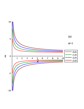
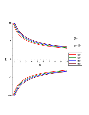
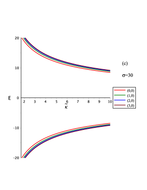
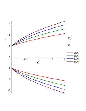
Figure 1: The energy levels in Eq.s (33), along with (32), for the KG-oscillators in EiBI-gravity with the Ricci scalar curvature and a WYMM. The corresponding $\left(n_{r},\ell\right)$- states, for $\ell=0$ and $n_{r}=0,1,2,3$, are plotted for $m_{\circ}=1$, $\alpha=0.5$, $\xi=1/6$ (a) at $\sigma=1$ against different Eddington parameter $\tilde{\kappa}>0$ values, (b) at $\sigma=10$ against different Eddington parameter $\tilde{\kappa}>0$ values, (c) at $\sigma=30$ against different Eddington parameter $\tilde{\kappa}>0$ values, and (d) at $\sigma=1$, against different KG-oscillators’ frequencies $\Omega>0$.

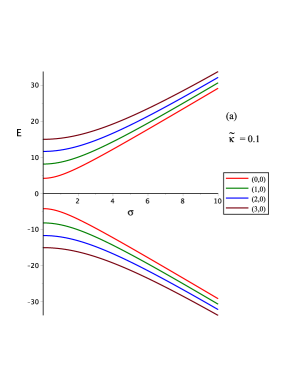
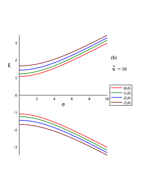
Figure 2: The energy levels in Eq.s (33), along with (32), for the KG-oscillators in EiBI-gravity with the Ricci scalar curvature and a WYMM. The corresponding $\left(n_{r},\ell\right)$- states, for different $\ell$ and $n_{r}$ values, for $\ell=0$ and $n_{r}=0,1,2,3$, at $m_{\circ}=1$, $\alpha=0.5$, $\xi=1/6$ (a) at $\tilde{\kappa}=0.1$ against WYMM strength $\sigma\geq 0$ values, and (b) at $\tilde{\kappa}=10$ against against WYMM strength $\sigma\geq 0$ values.

In Figure 1, we plot the energy levels in Eq.s (33), along with (32), for the KG-oscillators in EiBI-gravity with the Ricci scalar curvature and a WYMM. The corresponding $\left(n_{r},\ell\right)$- states, for $\ell=0$ and $n_{r}=0,1,2,3$, for $m_{\circ}=1$, $\alpha=0.5$, and $\xi=1/6$. The energy levels against different Eddington parameter $\tilde{\kappa}>0$ values are shown for $\sigma=1$, $\sigma=10$, and $\sigma=30$, in 1(a), 1(b), and 1(c), respectively. In 1(d) we show the energy levels at $\sigma=1$, against different KG-oscillators’ frequencies $\Omega>0$. In Figure 2, the energy levels are plotted against the WYMM strength $\sigma\geq 0$ at $\tilde{\kappa}=0.1$ and $\tilde{\kappa}=10$ in 2(a) and 2(b), respectively. Whereas, for different $\left(n_{r},\ell\right)$- states, the energies are plotted against different Eddington parameter $\tilde{\kappa}>0$ values at WYMM strengths $\sigma=1$ and $\sigma=10$ (in 3(a) and 3(b), respectively), and against different WYMM strength $\sigma\geq 0$ at the Eddington parameter $\tilde{\kappa}=0.1$ and $\tilde{\kappa}=10$, (3(c) and 3(d), respectively).

Obviously, all figures indicate that the energy gap between positive and negative energy levels is preserved. Such an energy gap is observed to decrease with increasing Eddington parameter $\tilde{\kappa}$ (as in Fig.s 1(a), 1(b), 1(c), 3(a) and 3(b)), where clustering of the energy levels, around $E=\pm m_{\circ}$, is observed eminent for extreme Eddington gravity, $\tilde{\kappa}>>1$. This is, in fact, the asymptotic tendency of the energy levels in (33), along with (32), at $\tilde{\kappa}>>1$. The energy gap, on the other hand, increases with increasing KG-oscillators’ frequency $\Omega$ (as in Fig. 1(d)), and with increasing WYMM strength $\sigma$ ( as in Fig.s 2(a), 2(b), 3(c), and 3(d)). Moreover, one observes that the separation between the energy levels as well as the KG-oscillator energies decrease with increasing values of the WYMM (documented in 1(a), 1(b), 1(c), 1(d), 3(a), and 3(b)). One would anticipate that at extreme WYMM strength (i.e., $\sigma>>1$) all quantum states would gather and collapse into one state (documented in 1(a), 1(b), 1(c), 3(a), and 3(b)).

At this point, one should be aware that the truncation of the confluent Heun function into a polynomial of order $n_{r}+1$ should be associated with some correlations/conditions. The use of such correlations is mandatory. We have just presented one of the many feasible correlations, to come out with a conditionally exact solution, in addition to those reported by Ishkhanyan ref71 . In what follows we shall show how quite flexible and handy the usage of the above methodical proposal is. We do so through the following illustrative examples.

III.2 KG-oscillators in GM-spacetime without EiBI-gravity, $\tilde{\kappa}=0$, and without Ricci scalar curvature effects

In no EiBI-gravity, $\tilde{\kappa}=0$, and without the Ricci scalar curvature effect, $\xi=0$, the first condition in (28) vanishes while the second term, since $C_{0}\neq 0$, implies that

$$\nu\left(\nu+\frac{1}{2}\right)-\mathcal{\tilde{P}}_{2}=0\Longrightarrow\nu=\frac{\mathcal{\tilde{L}}}{2},$$ (40)

where, in this case,

$$\mathcal{P}_{1}=\tilde{E}^{2}-3\Omega,\,\mathcal{P}_{2}=\mathcal{\tilde{L}}\left(\mathcal{\tilde{L}+}1\right);\,\mathcal{\tilde{P}}_{i}=\frac{\mathcal{P}_{i}}{4},\,\mathcal{\tilde{P}}_{2}=\frac{\mathcal{P}_{2}}{4},\,$$ (41)

and

$$\mathcal{\tilde{L}}=-\frac{1}{2}+\sqrt{\frac{1}{4}+\frac{\ell\left(\ell+1\right)-\sigma^{2}}{\alpha^{2}}},\,\tilde{E}^{2}=\frac{E^{2}-m_{\circ}^{2}}{\alpha^{2}}-3\Omega.$$ (42)

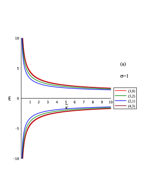
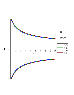
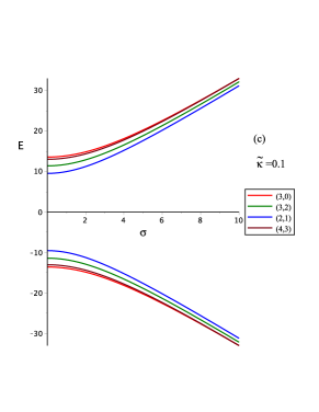
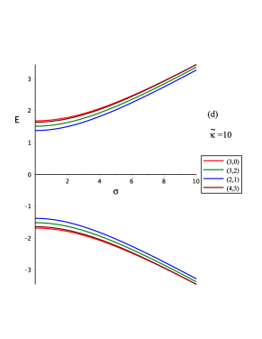
Figure 3: The energy levels in Eq.s (33), along with (32), for the KG-oscillators in EiBI-gravity with the Ricci scalar curvature and a WYMM. The energies are for different $\left(n_{r},\ell\right)$- states, for $m_{\circ}=1$, $\alpha=0.5$, $\xi=1/6$ (a) at $\sigma=1$, against different Eddington parameter $\tilde{\kappa}>0$ values, (b) at $\sigma=10$ against different Eddington parameter $\tilde{\kappa}>0$ values, (c) at $\tilde{\kappa}=0.1$ against different WYMM strength $\sigma\geq 0$ values, and (d) at $\tilde{\kappa}=10$ against different WYMM strength $\sigma\geq 0$ values.

Moreover, the L.H.S. of (29) is zero to yield

$$C_{j+1}\left[\mathcal{\tilde{P}}_{2}-\left(j+\nu+1\right)\left(j+\nu+\frac{3}{2}-\Omega\,\tilde{\kappa}\right)\right]=C_{j}\,\left[\mathcal{\tilde{P}}_{1}-\Omega\left(j+\frac{\mathcal{\tilde{L}}}{2}\right)\right]$$ (43)

We may now truncate the power series into a polynomial of order $n_{r}\geq 0$ by requiring that $\forall j=n_{r}$ we have $C_{n_{r}+1}=0$, and $C_{n_{r}}\neq 0$. Consequently,

$$\mathcal{\tilde{P}}_{1}=\Omega\left(n_{r}+\frac{\mathcal{\tilde{L}}}{2}\right)\Longrightarrow\tilde{E}^{2}=2\Omega\left(2n_{r}+\mathcal{\tilde{L}+}\frac{3}{2}\right)\Longrightarrow E=\pm\sqrt{2\Omega\alpha^{2}\left(2n_{r}+\mathcal{\tilde{L}+}3\right)+m_{\circ}^{2}}$$ (44)

This special case represents KG-oscillators in GM-spacetime and a WYMM and is in exact accord that in Eq.(31) of ref017 . Moreover, the radial wave function reads

$$R\left(y\right)=y^{\mathcal{\tilde{L}}/2}\sum\limits_{j=0}^{n_{r}}C_{j}y^{j}\Leftrightarrow R\left(r\right)=r^{\mathcal{\tilde{L}}}\sum\limits_{j=0}^{n_{r}}C_{j}\,r^{2j}$$ (45)

III.3 KG-oscillators in GM-spacetime without EiBI-gravity, $\tilde{\kappa}=0$, and with the Ricci scalar curvature effect

Without EiBI-gravity, $\tilde{\kappa}=0$, in the presence of the Ricci scalar curvature, $\xi\neq 0$, equation (27) results

$$\sum\limits_{j=0}^{\infty}\left\{C_{j}\,\left[\mathcal{\tilde{P}}_{1}-\Omega\left(j+\nu\right)\right]+C_{j+1}\left[\left(j+\nu+1\right)\left(j+\nu+\frac{3}{2}\right)-\mathcal{\tilde{P}}_{2}\right]\right\}y^{j+\nu+1}$$

$$+C_{0}\left[\nu\left(\nu+\frac{1}{2}\right)-\mathcal{\tilde{P}}_{2}\right]y^{\nu}=0.$$ (46)

Which would suggest that since $C_{0}\neq 0$ we have

$$\nu\left(\nu+\frac{1}{2}\right)-\mathcal{\tilde{P}}_{2}=0\Longrightarrow\nu=\frac{\mathcal{\tilde{L}}}{2},$$ (47)

where

$$\mathcal{\tilde{L}}=-\frac{1}{2}+\sqrt{\frac{1}{4}+\frac{\ell\left(\ell+1\right)-\sigma^{2}+2\xi\left(1-\alpha^{2}\right)}{\alpha^{2}}}.$$ (48)

Consequently, the truncation of our power series into a polynomial of order $n_{r}$ is secured by the requirement that $\forall j=n_{r}$ we have $C_{n_{r}+1}=0$, $C_{n_{r}}\neq 0$, and therefor4e

$$\mathcal{\tilde{P}}_{1}-\Omega\left(n_{r}+\nu\right)=0\Longrightarrow\frac{\tilde{E}^{2}-3\Omega}{4}=\Omega\left(n_{r}+\frac{\mathcal{\tilde{L}}}{2}\right)\Longrightarrow\frac{E^{2}-m_{\circ}^{2}}{\alpha^{2}}-6\Omega=4\Omega\left(n_{r}+\frac{\mathcal{\tilde{L}}}{2}\right),$$ (49)

to imply

$$E=\pm\sqrt{m_{\circ}^{2}+4\Omega\alpha^{2}\left(n_{r}+\frac{\sqrt{\alpha^{2}+4\ell\left(\ell+1\right)-4\sigma^{2}+8\xi\left(1-\alpha^{2}\right)}}{4\alpha}+\frac{5}{4}\right)}.$$ (50)

This result is in exact accord with that reported in Eq.(38) by Bragança et al. Re11 without the WYMM (i.e for $\sigma=0$). Again, the radial wave function reads

$$R\left(y\right)=y^{\mathcal{\tilde{L}}/2}\sum\limits_{j=0}^{n_{r}}C_{j}y^{j}\Leftrightarrow R\left(r\right)=r^{\mathcal{\tilde{L}}}\sum\limits_{j=0}^{n_{r}}C_{j}\,r^{2j}$$ (51)

III.4 KG-oscillators with EiBI-gravity, $\tilde{\kappa}\neq 0$, and without Ricci scalar curvature effect

For this case, one would use the first condition in (28) to obtain, since $C_{0}\neq 0$,

$$\left[\tilde{\kappa}\nu^{2}\right]=0\Longrightarrow\nu=0,$$ (52)

and use the second condition in (28) to imply

$$C_{1}=\frac{\tilde{P}_{2}}{\tilde{\kappa}}C_{0}\;$$ (53)

where

$$\mathcal{\tilde{P}}_{2}\rightarrow\tilde{P}_{2}=\tilde{\ell}\left(\tilde{\ell}+1\right)+2\Omega\,\tilde{\kappa},\,\tilde{\ell}=-\frac{1}{2}+\sqrt{\frac{1}{4}+\frac{\ell\left(\ell+1\right)-\sigma^{2}}{\alpha^{2}}-2\Omega\,\tilde{\kappa}},$$ (54)

and

$$C_{j+2}\left[\tilde{\kappa}\left(j+2\right)^{2}\right]=C_{j}\,\left[\Omega\,j-\mathcal{\tilde{P}}_{1}\right]+C_{j+1}\left[\tilde{P}_{2}-\left(j+1\right)\left(j+\frac{3}{2}-\Omega\,\tilde{\kappa}\right)\right].$$ (55)

Next, we truncate our power series in (26) into a polynomial of order $n_{r}+1=n\geq 1$ so that $\forall j=n_{r}$ we require $C_{n_{r}+2}=0$, $C_{n_{r}+1}\neq 0$, and $C_{n_{r}}\neq 0$. However, to facilitate the so called conditionally exact solvability, of the problem at hand, one would enforce the valid/viable assumptions that $\tilde{P}_{2}-\left(n_{r}+1\right)\left(n_{r}+\frac{3}{2}-\Omega\,\tilde{\kappa}\right)=0$ and $\Omega n_{r}-\mathcal{\tilde{P}}_{1}=0$. Under such assumptions, one would, respectively, obtain

$$\Omega\,\tilde{\kappa}=\frac{\alpha^{2}\left[2n_{r}\,\left(2n_{r}+5\right)+6\right]+\sigma^{2}-\ell\left(\ell+1\right)}{2\alpha^{2}\left(2n_{r}+4\right)},$$ (56)

and

$$\tilde{E}^{2}=2\Omega\left(2n_{r}+\frac{3}{2}\right)-\Omega^{2}\,\tilde{\kappa}\Longleftrightarrow E=\pm\sqrt{m_{\circ}^{2}+2\Omega\alpha^{2}\left(2n_{r}+3\right)}.$$ (57)

One may observe that our results in (56) and (57) are in exact accord with those reported in Eq.s (41) and (43) of ref701 . In this case, moreover, the radial wave function reads

$$R\left(y\right)=\sum\limits_{j=0}^{n_{r}+1}C_{j}y^{j}\Leftrightarrow R\left(r\right)=\sum\limits_{j=0}^{n_{r}+1}C_{j}\,r^{2j}$$ (58)

IV Concluding remarks

We have studied and investigated KG-oscillators in a GM spacetime in EiBI-gravity, including a WYMM and the Ricci scalar $R=R_{\upsilon}^{\upsilon}$ effects. In the light of our investigation, our observations are in order.

In connection with the quantum mechanical central repulsive core, $\mathcal{\ell}\left(\ell+1\right)/r^{2}\longrightarrow\mathcal{\tilde{L}}\left(\mathcal{\tilde{L}+}1\right)/r^{2}$, where $0\leq\mathcal{\tilde{L}}\in\mathbb{R}$ identifies a new irrational orbital quantum number, we recollect (from Eq. (15)) that

$$\frac{\mathcal{\tilde{L}}\left(\mathcal{\tilde{L}+}1\right)}{r^{2}}=\frac{\ell\left(\ell+1\right)-\sigma^{2}+2\xi\left(1-\alpha^{2}\right)}{\alpha^{2}r^{2}}+\frac{2\Omega\,\tilde{\kappa}}{r^{2}}.$$ (59)

It is clear that the inclusion of the Ricci scalar curvature $R$ and EiBI-gravity, manifestly and effectively, introduce an additional repulsive force fields, $\frac{2\xi\left(1-\alpha^{2}\right)}{\alpha^{2}r^{2}}$ and $\frac{2\Omega\,\tilde{\kappa}}{r^{2}}$, respectively. Whereas an attractive force field is introduced by the WYMM, $-\frac{\sigma^{2}}{r^{2}}$. The competitions between such fields identifies the allowed orbital $\ell$ excitations, provided that $0\leq\ell\in\mathbb{R}$, as documented in (35). One should keep in mind, moreover, that $\mathcal{\tilde{L}}=\ell$ for $\sigma=\xi=\tilde{\kappa}=0$ and $\alpha=1$ (i.e., flat Minkowski spacetime).

As to the effects on the spectroscopic structure of the KG-oscillators in a GM spacetime in EiBI-gravity, in a WYMM and the Ricci scalar curvature, we have observed that the energy gap, between positive and negative energy levels, decreases with increasing Eddington parameter $\tilde{\kappa}$ (documented in Fig.s 1(a), 1(b), 1(c), 3(a) and 3(b)). Yet, the energy levels tend to cluster around $E=\pm m_{\circ}$ for extreme Eddington gravity (i.e., $\tilde{\kappa}>>1$), which, in fact, reflects the asymptotic tendency of the energy levels in (33), along with (32), at $\tilde{\kappa}>>1$. Whereas, the energy gap increases with increasing KG-oscillators’ frequency $\Omega$ (documented in Fig. 1(d)), as well as with increasing WYMM strength $\sigma$ ( documented in Fig.s 2(a), 2(b), 3(c), and 3(d)). Moreover, we have observed that the separation between the energy levels (among positive or among negative energy states) as well as the KG-oscillator energies decrease with increasing values of the WYMM strength $\sigma$ (documented in 1(a), 1(b), 1(c), 1(d), 3(a), and 3(b)). One would anticipate that at extreme WYMM strength (i.e., $\sigma>>1$) all quantum states would cluster and collapse into one state (documented in 1(a), 1(b), 1(c), 3(a), and 3(b)). Yet, one may observe the competition between EiBI-gravitational field and the gravitational field introduced by Ricci scalar curvature in Fig.s 2(a) and 2(b). Whilst the increase in the Eddington parameter (i.e., stronger Eddington gravity) $\tilde{\kappa}>>1$ lowers the particle/anti-particle energies, the increase in the WYMM strength $\sigma$ increases the particle/anti-particle energies. The same trend of effects holds true for states with different $(n_{r},\ell)$ as shown in Fig.s 3(a), 3(b), 3(c), and 3(d).

Finally. the solutions of some relativistic and non-relativistic quantum mechanical systems, that are of quantum gravity and/or astroparticle physics interest, are often given in terms of the confluent Heun $H_{C}\left(\alpha,\beta,\gamma,\delta,\eta,z\right)$ and biconfluent Heun $H_{B}\left(\alpha,\beta,\gamma,\delta,z\right)$ functions. The power series expansion of which yields a three terms recursion relations similar to Eq. (29). The truncation of such power series into polynomials of order $n_{r}+1$ is a mandatory requirement, so that such solutions are physically admissible, finite and square integrable ones. For example, the truncation the confluent Heun $H_{C}\left(\alpha,\beta,\gamma,\delta,\eta,z\right)$ is secured by the condition $\delta=-\alpha\left(n_{r}+\left[\beta+\gamma+2\right]/2\right)$ (c.f., e.g., ref701 ; ref71 ). Ishkhanyan et al. ref71 ) have discussed some conditions to be fulfilled for such truncation condition. We, in the current methodical proposal, have introduce yet another alternative condition (i.e., $C_{n_{r}+2}=0$, $C_{n_{r}+1}\neq 0$, and $C_{n_{r}}\neq 0$ reported for our result in (32) and (33)). that allows such a truncation recipe to be valid/viable and facilitates conditional exact solvability of the problem at hand. The same procedure can be followed for the biconfluent Heun $H_{B}\left(\alpha,\beta,\gamma,\delta,z\right)$ functions as well. Under such proposal setting (reported in subsection 3-A), one gets conditional exact solutions for a set of quantum mechanical states that are correlated with some condition like that reported in (32). To facilitate the convergence of the solution into special, less complicated though, interesting spacetime background models, the reader is advised to follow simple expansion variable that allows such convergence (like the change of variables $y=r^{2}$ used to obtain (20)). Such special spacetime background models work as controlling mechanism on the correctness of the reported solution of the more complicated one. This is documented in subsections 3(b), 3(c), and 3(d).

References

• (1) T W B Kibble, Phys. Rep. 67 (1980) 183.
• (2) M. Barriola, A. Vilenkin, Phys. Rev. Lett. 63 (1989) 341.
• (3) A. Vilenkin, Phys. Rep. 121 (1985) 263.
• (4) A. Vilenkin, Phys. Rev. D 23 (1981) 852.
• (5) A. Vilenkin, Phys. Rev. Lett. 46 (1988) 1169.
• (6) A. Vilenkin, Phys. Lett. B 133 (1983) 177.
• (7) W A Hiscock, Phys. Rev. D 31 (1985) 3288.
• (8) B Linet, Gen. Relativ. Gravit. 17 (1985) 1109,
• (9) A L Cavalcanti de Oliveira, E R Bezerra de Mello, Class Quant. Grav. 23 (2006) 5249.
• (10) T.R.P. Caramês, J.C. Fabris, E R Bezerra de Mello, H Belich, Eur. Phys. J. C 77 (2017) 496.
• (11) R L L Vitória, H Belich, Phys. Scr. 94 (2019) 125301.
• (12) O. Mustafa, Ann. Phys. 459 (2023) 169550.
• (13) C Furtado, F Moraes, J. Phys. A: Math. Gen. 33 (2000) 5513.
• (14) T.R.P. Caramês, J.C. Fabris, E R Bezerra de Mello, H Belich, Eur. Phys. J. C 77 (2017) 496.
• (15) T T Wu, C N Yang, Nucl. Phys. B 107 (1976) 365.
• (16) T T Wu, C N Yang, Phys. Rev. D 12 (1975) 3845.
• (17) E R Bezerra de Mello, Class. Quant. Grav. 19 (2002) 5141.
• (18) J Spinelly, U de Freitas, E R Bezerra de Mello, Phys. Rev. D 66 (2002) 024018.
• (19) A. Edery and Y. Nakayama, Phys. Rev. D 98 (2018) 064011.
• (20) E A F Bragança, R L L Vitória, H Belich, E R Bezerra de Mello, Eur. Phys. J. C 80 (2020) 206.
• (21) M Moshinsky, A Szczepaniak, J. Phys. A: math. Gen. 22 (1989) L817.
• (22) B Mirza, M Mohandesi, Commun. Theor. Phys. 42 (2004) 664.
• (23) K Bakke, H F Mota, Eur. Phys. J. Plus 133 (2018) 409.
• (24) A Boumali, H Aounallah, Adv. High Energy Phys. 2018 (2018) 1031763.
• (25) G A Marques, E R Bezerra de Mello, Class. Quant. Gravit. 19 (2002) 985.
• (26) S S Alves, M M Cunha, H Hassaabadi, E O Silva, Universe 9 (2023) 132.
• (27) E R Bezerra de Mello, C Furtado, Phys. Rev. D 56 (1997) 1345.
• (28) F. Ahmed, Phys. Scr. 98 (2023) 015403.
• (29) F. Ahmed, Sci. Rep. 12 (2022) 8794.
• (30) J Cravalho, C Furtado, F Moraes, Phys. Rev. A 84 (2011) 032109.
• (31) N A Rao, B A Kagali, Mol. Phys. Lett. A 19 (2004) 2147.
• (32) K Bakke, C Furtado, Ann. Phys. 336 (2013) 489.
• (33) P Strange, L H Ryder, Phys. Lett. A 380 (2016) 3465.
• (34) O Mustafa, Ann. Phys. 440 (2022) 168857.
• (35) O Mustafa, Eur. Phys. J. C 82 (2022) 82.
• (36) O Mustafa, Ann. Phys. 446 (2022) 169124.
• (37) O Mustafa, Eur. Phys. J. Plus 138 (2023) 21.
• (38) O. Mustafa, Phys. Lett. B 839 (2023) 137793.
• (39) O. Mustafa, Nucl. Phys. B 995 (2023) 116334.
• (40) O. Mustafa, Int. J. Geom. Meth. Mod. Phys. 20 (2023) 2350221.
• (41) A Boumali, N Messai, Can. J. Phys. 92 (2014) 11.
• (42) K Bakke, C Furtado, Ann. Phys. 355 (2015) 48.
• (43) R L LVitória, H Belich, Eur. Phys. J. C 78 (2018) 999.
• (44) R L LVitória, K Bakke, Eur. Phys. J. Plus 133 (2018) 490.
• (45) R L LVitória, H Belich, K Bakke, Eur. Phys. J. Plus 132 (2017) 25.
• (46) J Cravalho, A M Cravalho, E Cavalcante, C Furtado, Eur. Phys. J. C 76 (2016) 365.
• (47) H. Hassanabadi, M. Hosseinpour, Eur. Phys. J. C 76 (2016) 553.
• (48) H. Hassanabadi, S Sargolzaeeipor, B H Yazarloo, Few-Body syst. 56 (2015) 115.
• (49) M. Banados, F. Ferreira, Phys. Rev. Lett. 105 (2010) 011101. Erratum:[Phys. Rev. Lett. 113 (2014) 119901].
• (50) S. Deser and G. W. Gibbons, Classical Quantum Gravity 15 (1998) L35.
• (51) D. N. Vollick, Phys. Rev. D 69 (2004) 064030.
• (52) T. Delsate, J, Steinhoff, Phys. Rev. Lett. 109 (2012) 021101.
• (53) R.D Lambaga, H S Ramadhan, Eur. Phys. J. C 78 (2018) 436.
• (54) P. Pani, V. Cardoso and T. Delsate, Phys. Rev. Lett. 107 (2011) 031101.
• (55) P.P. Avelino, Phys. Rev. D 85 (2012) 104053.
• (56) P. Pani, T. Delsate and V. Cardoso, Phys. Rev. D 85 (2012) 084020.
• (57) F. Fiorini and R. Ferraro, Int. J. Mod. Phys. A 24 (2009) 1686.
• (58) R. Ferraro and F. Fiorini, Phys. Lett. B 692 (2010) 206.
• (59) I. Gullu, T. C. Sisman and B. Tekin, Class. Quant. Grav. 27 (2010) 162001.
• (60) I. Gullu, T.C. Sisman and B. Tekin, Phys. Rev. D 82 (2010) 124023.
• (61) T. Clifton, P.G. Ferreira, A. Padilla and C. Skordis, Phys. Rept. 513 (2012) 1.
• (62) J. R. Nascimento, G. J. Olmo, P. J. Porfírio, A. Yu. Petrov, A. R. Soares, Phys. Rev. D 101 (2020) 064043.
• (63) C F S Rereira, A R Soares, R L L Vitória, H Belich, Eur. Phys. J. C 83 (2023) 270.
• (64) A R Soares, R L L Vitória, C F S Rereira, Eur. Phys. J. C 83 (2023) 903.
• (65) C F S Rereira, R L L Vitória, A R Soares, H Belich, Int. J. Theor. Phys. 62 (2023) 225.
• (66) O. Mustafa, A. R. Soares, C. F. S. Pereira, R. L. L. Vitória, arXiv:2401.09502 ”On the Klein-Gordon oscillators in Eddington-inspired Born-Infeld gravity global monopole spacetime and a Wu-Yang magnetic monopole”, (2024).
• (67) T A Ishkhanyan, V P Krainov, A M Ishkhanyan, J. Phys.: Conf. Series 1416 (2019) 012014.
• (68) A V Turbiner, Phys. Rep. 642 (2016) 1.
• (69) F. dos S. Azevedo, J. D. M. de Lima, A. de Pādua, F. Moraes, Phys. Rev. A 103 (2021) 023516.
• (70) Q. G. Garcia, P. J. Porfírio, D. C. Moreira, C. Furtado, Nucl. Phys. B 950 (2020) 114853.
• (71) G. J. Olmo, D. Rubiera-Garcia, Int. J. Mod. Phys.D 24 (1015) 1542013.
• (72) J. R. Nascimento, G. J. Olmo, A. Yu. Petrov, P. J. Porfírio, A. R. Soares, Phys. Rev. D 99 (2019) 064053.
• (73) H. Aounallah, A. R. Soares, R L LVitória, Eur. Phys. J. C 80 (2020) 447.
• (74) A. R. Soares, R L LVitória, H. Aounallah, Eur. Phys. J. Plus 136 (2021) 966.
• (75) T. Müller, Phys. Rev. D 77 (2008) 044043.
• (76) F. Ahmed, Few-Body syst. 64 (2023) 80.
• (77) O. Mustafa, arXiv:2310.10122 ”Klein-Gordon particles in a quasi-pointlike global monopole spacetime and a Wu-Yang magnetic monopole: invariance and isospectrality”.
• (78) O. Mustafa, Ann. Phys. 459 (2023) 169550.