Weakly nonlinear analysis of Turing pattern dynamics on curved surfaces
Abstract
Pattern dynamics on curved surfaces are ubiquitous. Although the effect of surface topography on pattern dynamics has gained much interest, there is a limited understanding of the roles of surface geometry and topology in pattern dynamics. Recently, we reported that a static pattern on a flat plane can become a propagating pattern on a curved surface [Nishide and Ishihara, Phys. Rev. Lett. 2022]. By examining reaction-diffusion equations on axisymmetric surfaces, certain conditions for the onset of pattern propagation were determined. However, this analysis was limited by the assumption that the pattern propagates at a constant speed. Here, we investigate the pattern propagation driven by surface curvature using weakly nonlinear analysis, which enables a more comprehensive approach to the aforementioned problem. The analysis reveals consistent conditions of the pattern propagation similar to our previous results, and further predicts that rich dynamics other than pattern propagation, such as periodic and chaotic behaviors, can arise depending on the surface geometry. This study provides a new perspective on the relationship between surfaces and pattern dynamics and a basis for controlling pattern dynamics on surfaces.
I Introduction
Pattern formation occurs at a wide range of scales in natural and engineered systems, including nanoscale metal stripes, chemical waves, fish and animal skin, vegetation, and atmospheric convection [4, 1, 2, 5, 3, 6, 7, 8]. The stages in which pattern formation occurs are diverse in terms of spatial dimensions and geometries, among which curved surfaces are common and fundamental. In particular, biological systems are rich sources of pattern dynamics on curved surfaces [9, 10, 12, 13, 14, 15, 11]. Recent developments in experimental techniques for measuring and controlling curved surfaces have revealed the functional roles of curved surfaces in pattern formation [16, 17, 18]. Bin/Amphiphysin/Rvs domain proteins sense the curvature of cellular membranes and regulate the cellular shape [19, 20]. The distribution of the mechanosensitive protein Piezo1 is regulated by membrane curvature [21]. Cellular migration is guided by the curvature of a substrate and is called “curvotaxis” [22]. The thickness of a cellular sheet depends on the curvature of the substrate [23].
Several theoretical studies have revealed the effects of geometry and topology on pattern formation and dynamics. Geodesic curvature causes the splitting [24], rectification [25], and swirling [26, 27, 14] of excitable waves and variations in the wavefront speed [30, 28, 29]. It also controls the position of the localization pattern [31, 32]. The rectification of propagating patterns by curved surfaces was also reported in the collective motion of self-propelled particles [33]. For pattern dynamics described by polar and nematic variables, topological defects are constrained by Poincaré–Hopf theorem on closed surfaces [34], and have been investigated in liquid crystals [35, 36], flocking [37], and active nematics [38]. This restriction plays a critical role in hydra regeneration, where singular points of cortical actin fibers dictate the positional information of morphogenesis [15].
Turing patterns, a prominent example of pattern formation [39, 40, 41, 42], have also attracted much interest in their dynamics on curved surfaces; in fact, Turing himself studied the pattern on a sphere to consider embryogenesis [39]. Since then, Turing patterns have been studied on several curved surfaces [43, 44, 46, 45]: spheres [39, 47, 48, 49, 50, 51], hemispheres [52, 53], tori [54, 51], ellipsoids [54, 55], and deformed axisymmetric cylinders and spheres [56]. These studies have reported that the profile and position of a Turing pattern change to reflect the surface shape. For example, Frank et al. studied pattern formation on a cylinder with a ridge, and found that the stripe pattern position is modulated by the ridge, termed as “pinning” [56]. All these studies presumed that a Turing pattern, which is static on a flat plane, remains static irrespective of the surface geometry.
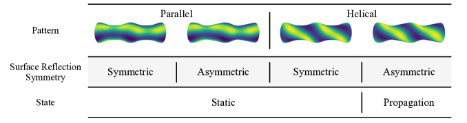
We recently reported that a Turing pattern can no longer remain static on curved surfaces [57], indicating a new mechanism of pattern propagation caused by surface curvature, i.e., a pattern that is static on a flat plane propagates on a curved surface. We primarily studied patterns on axisymmetric surfaces, which enabled a tractable analysis. Linear stability analysis indicates no sign of Hopf bifurcation, similar to the standard Turing instability condition, and the growth rate near the uniform state is indistinguishable between flat planes and curved surfaces (see Sec. II.2). Thus, analysis incorporating nonlinearity is required to understand the onset of such time-dependent dynamics. We performed numerical simulations and theoretical analyses based on the relationship between the propagation velocity and the pattern profile (see Eq. (7) in Sec. II.3) and revealed that the onset of propagation is conditioned by symmetries of the surface and pattern. The helical pattern propagates unless the surface is reflection-symmetric, whereas the parallel pattern is always static (see Fig. 1). These results are generic and were confirmed by numerical simulations of the Brusselator [58, 59] and Lengyel–Epstein [60, 61] models.
In this paper, we adopt an alternative analysis method to uncover the manner in which a static pattern on a plane can propagate on a curved surface. Our previous analysis assumed that patterns propagate at a constant velocity along the azimuthal direction and used the relationship in Eq. (7). Instead, in this study, we consider the solution of the reaction-diffusion equation (RDE) in the vicinity of the Turing bifurcation point and perform a weakly nonlinear analysis. Near the bifurcation point, the amplitudes of the pattern profile are small, which allows us to expand the pattern by the superposition of a few linear modes and derive the amplitude equations [62, 59, 63, 64, 46]. The obtained amplitude equations indicate that different mode-mode interactions occur depending on the symmetries of the surface and pattern profile, resulting in either the onset or suppression of pattern propagation. This analysis not only leads to consistent results as in [57], but further predicts that non-trivial dynamics other than propagating patterns, including periodic and chaotic behaviors, can appear on curved surfaces. These results are confirmed by numerical simulations.
This paper is organized as follows. Sec. II describes the setup of our problem, and summarizes our previous results that the Turing pattern can propagate on a curved surface. In Sec. III, the amplitude equations for the RDE on an axisymmetric surface are discussed. Possible forms of amplitude equations depending on the surface and pattern symmetries are determined. In Sec. IV, the correspondence between the steady-state solutions of the amplitude equations and static and propagating patterns is discussed. In Sec. V, the amplitude equations for the Brusselator model are derived and the discussions in the previous sections are numerically confirmed. Sec. VI shows that surface curvature can cause diverse pattern dynamics other than propagation, which is a summary of the joint paper [65]. Finally, the results are summarized in Sec. VII.
II Model and Propagating Pattern
II.1 Model
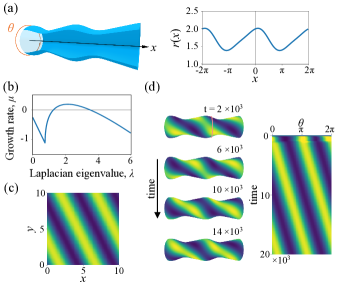
We study reaction-diffusion systems on an axisymmetric surface represented by (Fig. 2(a)). The coordinates and are defined as and , respectively, and periodic boundary conditions are used for both axes unless otherwise mentioned. We consider the general form of the RDE as follows:
| (1) |
where is the vector representation of the chemical concentrations and a function of the position on the surface and the time , is a diagonal matrix composed of the diffusion coefficients, is the Laplace–Beltrami operator, and is the reaction term. The Laplace–Beltrami operator characterizes the effect of the surface curvature on the system [67]. In general, for a curved surface parameterized by the coordinates , the Laplace–Beltrami operator for a scalar-field variable is determined by the metric tensor , where we use the notation :
| (2) |
where, is the inverse of , , and we use the Einstein summation convention for repeated indices. For an axisymmetric surface, , , , and , where . The Laplace–Beltrami operator is given by:
| (3) |
We assume that Eq. (1) has a unique uniform steady solution, , that satisfies , and the steady-state solution becomes unstable because of the Turing instability indicated by the dispersion relation discussed below.
As a representative example, we use the Brusselator model given by
| (4) |
where and represent the chemical concentrations at the position on the surface and time , and are the diffusion coefficients of and , respectively, and and are model parameters. The Brusselator model has a uniform steady solution, , and, although it can show various spatiotemporal patterns including static stripes, spiral propagation, and oscillatory patterns [66], in this study we selected parameter sets such that the system exhibits a Turing pattern on a flat surface. For the numerical data presented in this study, we verified that the pattern is static on a flat plane. The details of the numerical simulation method are provided in Supplemental Text Sec. S1 [68].
II.2 Linear stability analysis
Turing instability is characterized by the dispersion relation , where is the eigenvalue of the Laplace–Beltrami operator. The dispersion relation is obtained by a linear stability analysis at the uniform state , as an eigenvalue of the linear operator
| (5) |
where denotes the Jacobian matrix of at . The eigenfunctions of are represented by , with the Laplace–Beltrami eigenfunction defined by . For flat surfaces, coincides with the square of the wavenumber. For an axisymmetric surface, can be factored into , where is the wavenumber along the -direction and is an integer. is a function of and is the solution to the following equation:
| (6) |
under the periodic boundary condition. Note that the eigenvalue is a nonnegative real number (), which is a general feature of the Laplace–Beltrami operator. In addition, the eigenvalues are discretized for a closed surface with a finite area. The eigenvalues are degenerate two-fold for , for which and are pairwise eigenfunctions that correspond to the anti-phase shift along the -axis. Vector is the eigenvector of the matrix , where is satisfied. The dispersion relation represents the growth rate of a mode characterized by . For Turing instability, takes real positive values within a finite range of , and the corresponding eigenvector is a real-valued vector. Note that the dispersion relation , and thus the Turing condition, is the same for any surface.
II.3 Pattern propagation on axisymmetric surface
By setting the parameters in the Brusselator model to , we obtain the dispersion relation shown in Fig. 2(b). In the numerical simulation of the RDE, the initial small fluctuation around the uniform solution grows and the chemical concentration eventually forms a spatially periodic pattern (i.e., the Turing pattern). The pattern is static on a plane (Fig. 2(c)), whereas it propagates on an axisymmetric surface, as shown in Fig. 2(d). Futhermore, the propagation is observed when the Neumann boundary condition is employed (Fig. S1 [68]).
The velocity of the pattern is related to the pattern profile and surface shape. Assuming a traveling wave solution with , the angular velocity along the -axis is obtained by the following equation:
| (7) |
where the inner product is defined by
| (8) |
with the area element , and denoting the Hermitian adjoint vector of .
In our previous study [57], we used Eq. (7) to reveal the relationship between pattern propagation and the symmetry of patterns and surfaces, as summarized in Fig. 1. The analysis therefore largely depended on the assumption that the pattern propagates at constant speed. Note also that we primarily studied axisymmetric surfaces with -periodicity along the -axis; in this study, we will show that the loss of the -periodicity results in the propagation of the parallel pattern.
III Amplitude equation and symmetry of system
III.1 Mode decomposition of the pattern dynamics
We analyze the propagating pattern on an axisymmetric surface by expanding the pattern using eigenfunctions of the linear operator in a uniform state, . If the pattern is not significantly far from the bifurcation point of the Turing instability, where the uniform solution becomes unstable, the pattern profile can be approximated by a linear combination of a few eigenfunctions . We evaluate the expansion coefficients by numerically calculating the inner product between the eigenfunction and the propagating pattern .
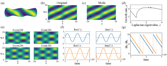
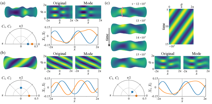
This expansion was applied to the numerically obtained Brusselator patterns (see Figs. 3 and S2–S4 [68]). The helical propagating pattern shown in Figs. 3(a) and (b) is well approximated by two pairwise eigenfunctions with the same wavenumber, . Fig. 3(c) shows the main part of the expansion:
| (9) | ||||
This closely approximates the original patterns and . Here, the complex coefficients and represent the amplitudes and phases of the corresponding modes, which are given by and , respectively. indicates the complex conjugate of . As is a real function, the coefficients of the pairwise eigenfunction are complex conjugates. Notably, a single pair of eigenfunctions, , is insufficient to express the helical pattern; at least two pairs of eigenfunctions are required. In the present example, the two eigenvalues are indicated by the colored dots in the dispersion relation shown in Fig. 3(d), and the corresponding eigenmodes are shown in Fig. 3(e). As the pattern propagates along the -axis, the coefficients of these modes, and , oscillate periodically with constant amplitudes and , respectively, and with the same frequency , where is the angular velocity of the pattern propagation (Figs. 3(f) and (g)). Thus, Eq. (9) can be expressed as
| (10) |
where and denote, respectively, the phases of and at . This expression indicates that the pattern propagates with a constant shape and velocity.
The static patterns are also well approximated by two pairwise eigenfunctions with the same wavenumber , where and are constants (Figs. S2–S4 [68]). Overall, these results indicate that the time evolution of the propagating pattern can be described by the coefficients for a few modes.
III.2 Amplitude equations for axisymmetric surfaces
Based on the observations earlier, we approximate a pattern on a surface using two pairs of eigenfunctions with the same wavenumber in the -direction as
| (11) |
where indicates the complex conjugate of the former terms, and the coefficients and are functions of time . We explore amplitude equations that describe the pattern dynamics on an axisymmetric curved surface.
| (12) | ||||
| (13) |
We mainly consider the situation in which two pairs of real eigenfunctions with the same , namely and , are relevant. This situation meets the aforementioned helical pattern and other cases (see Supplemental Text Sec. S4 for cases in which the two modes have different wavenumbers and [68]). In the vicinity of the Turing bifurcation point, the amplitudes of these modes, and , are both expected to be small, and the right-hand sides of the amplitude equations, and , can be expanded with respect to and [63]. The symmetries inherent in the system impose strong restrictions on the possible forms of the amplitude equations, as investigated in this section. The amplitude equations can also be derived from the original RDE using methods such as the reductive perturbation method [64]; we will carry out the derivation for the Brusselator model in Sec. V.
III.2.1 Amplitude equations for general axisymmetric surfaces
For an axisymmetric surface, the RDE is invariant about the translation by arbitrary along the -direction, , and the reflection about the -direction, :
| (14) | ||||
| (15) |
The actions of the transformations and on a pattern (see Eq. (11)) can be recast because their actions on the amplitudes are as follows:
| (16) | ||||
| (17) |
The amplitude equations, which are the reduction equations of RDE, should also be invariant to these transformations. Thus, the general form of the amplitude equations up to the third-order expansion of is given by
| (18) | ||||
| (19) |
where the coefficients and are real values owing to the invariance of the transformation . The second-order terms do not appear in the equations. The coefficients and coincide with growth rates and , respectively. The other coefficients are not determined solely by the discussion of symmetries given here. Below, we assume that the coefficients are chosen such that the solution does not diverge; otherwise, higher-order terms are required to prevent divergence.
Using the complex variables and as , the pattern profile in Eq. (11) can be written as
| (20) |
where the amplitudes, and , and phase variables, and , are real-valued functions of time . The amplitude equations can be rewritten as follows:
| (21) | ||||
| (22) | ||||
| (23) |
where we introduce the phase difference . These equations are closed in three variables, , , and , because the system is invariant for translation along the -axis. Note also that they are invariant under the transformation because the system has reflection-symmetry along the -axis. The phase variables and evolve according to the following equations:
| (24) | ||||
| (25) |
Eqs. (21)–(23), supplemented by Eqs. (24) and (25), constitute the general form of the amplitude equations for pattern dynamics on an axisymmetric surface. Note that the derived amplitude equations Eqs. (18) and (19) are also valid for non-Turing systems as long as the system satisfies similar conditions such as invariance to the transformations Eqs. (14) and (15).
III.2.2 Amplitude equations for reflection-symmetric surfaces
An axisymmetric surface can have additional symmetries. Here, we consider the case in which the surface is reflection-symmetric about the -axis, satisfying , where the origin of the -axis can be arbitrary because of the periodic boundary condition. For such a surface, RDE is invariant under the reflection about the -direction, :
| (26) |
The eigenfunctions of the Laplace–Beltrami operator are either even or odd with respect to . The action of the reflection on is dependent on the parity of and acts as
| (29) |
When and are both even or odd functions, the amplitude equations are the same as those in the general case of Eqs. (18) and (19). However, when and are a combination of even and odd functions, the amplitude equations are reduced to
| (30) | ||||
| (31) |
corresponding to the case and in Eqs. (18) and (19). The amplitude and phase variables obey
| (32) | ||||
| (33) | ||||
| (34) |
and
| (35) | ||||
| (36) |
III.2.3 Amplitude equations for -periodic surface along the -axis
The axisymmetric surface can be periodic along the -axis, satisfying , where is a constant smaller than the axial length of the surface. Here, we consider a simple case in which the surface is -periodic (as in our previous study [57]), satisfying , and the domain of is defined as . For such a surface, the RDE is invariant to the -translation along the -axis and is defined as
| (37) |
and reflection about the -direction, . According to Bloch’s theorem [71], the eigenfunctions of the Laplace–Beltrami operator either change sign or remain unchanged by the action of .
| (38) |
The action of -translation on act as
| (41) |
When and both undergo the same transformation by , the amplitude equations are the same as those in the general case of Eqs. (18) and (19). Conversely, when and undergo transformations of different signs by , the amplitude equations are the same as those on the reflection-symmetric surface in Eqs. (30) and (31).
III.2.4 Patterns consisting of single paired modes
The patterns can be dominated by only a single paired mode, as exemplified in Fig. 4, where the amplitudes of the other modes decrease.
| (42) |
The pattern is always reflection-symmetric around the -axis as where the origin of the -axis is properly chosen. Based on the invariance by the transformations and , the amplitude equation is given by
| (43) |
where coincides with the growth rate and is supposed to be a negative real value. With , we obtain:
| (44) | ||||
| (45) |
These equations indicate that the pattern does not exhibit propagation.
III.2.5 Patterns on a flat surface
Summarizing the analysis for the flat surface case is helpful. On the -plane, the pattern can be expanded by using the Fourier mode . The stripe pattern resulting from Turing instability (Fig. 2) comprises at most two paired modes and is approximated by
| (46) |
The amplitude equations are derived by considering that the plane is invariant to translations and reflections:
| (47) | ||||
| (48) |
Then, amplitudes and phases obey
| (49) | ||||
| (50) | ||||
| (51) |
and pattern propagation is not possible. In the case of a plane, coupling with higher-order harmonic modes such as and can result in propagating waves, even in a one-dimensional (1D) system [63]. We ignore such situations because they generally occur far from the Turing bifurcation point and depend on the specific nature of the system, such as domain size (see Supplemental Text Sec. S4 [68]).
IV Steady-state solutions of amplitude equations
Here, we investigate the steady-state solutions of the amplitude equations derived in the preceding section: . For the given solution, the symmetries of the corresponding patterns and phase velocities are determined. As a pattern of single paired modes cannot propagate (see Eq. (45)), we consider the case in which two pairs of modes are relevant and and are assumed to be non-zero.
IV.1 Steady-state solutions of Eqs. (32)–(34)
The amplitude equations (32)–(34) are obtained for the reflection-symmetric surface with eigenfunctions that have different parities as and (Sec. III.2.2), or for a -periodic surface with eigenfunctions that transform differently as and (Sec. III.2.3). In the steady-state, either of the following relationships should hold from Eq. (34):
| (52) | |||
| (53) |
For the solution (Eq. (52)), the phase equations in Eqs. (35) and (36) satisfy , indicating that this solution represents a static pattern. The profile of the pattern is expressed as
| (54) | ||||
| (55) |
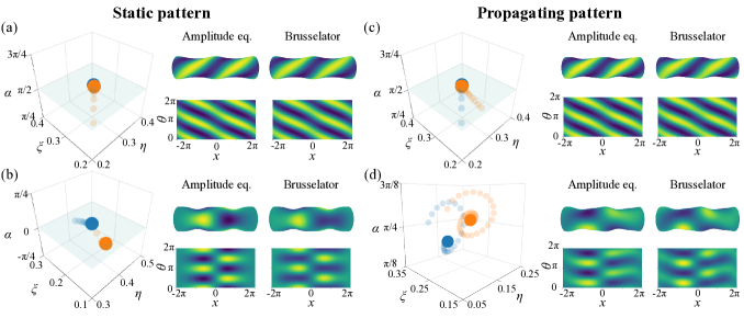
where and is a constant determined by the initial condition. When , the pattern is reflection-symmetric along the -axis, satisfying . Fig. 5(a) shows an example of a -periodic surface, where we set . In the other case, , the pattern symmetry depends on the surface symmetry. On reflection-symmetric surfaces, the pattern is inversion-symmetric, satisfying . On -periodic surfaces, the pattern is invariant against the simultaneous transformation of reflection about the -axis and -translation along the -axis, satisfying . Fig. 5(b) shows an example of the case on a reflection-symmetric surface ().
For the steady-state solution given by Eq. (53), the phase velocities and are generally non-zero and constant (), indicating a propagating pattern. The pattern shows neither reflection- nor inversion- symmetry because of the superposition of the two paired modes in . This non-trivial solution was omitted in the previous approach [57]. Fig. 5(c) shows an example of a propagating pattern on a -periodic surface (). This non-trivial solution is absent on a flat-plane where (see Eqs. (47) and (48)).
IV.2 Steady-state solutions of Eqs. (21)–(23)
Next, we consider the steady-state solutions of the general amplitude equations given by Eqs. (21)–(23). The equations are obtained for a general axisymmetric surface (Sec. III.2.1), for cases in which and are both even or odd functions on a reflection-symmetric surface (Sec. III.2.2), or when and are transformed with the same sign by -translation along the -axis on a -periodic surface (Sec. III.2.3). In the steady-state, Eq. (23) yields to either of the following solutions:
| (56) | |||
| (57) | |||
| (58) |
From Eqs. (24) and (25), the first solution represents a static pattern whereas the others represent propagating patterns. Note that at , the solutions Eqs. (57) and (58) coincide with the solutions included in Eq. (52) and Eq. (53), respectively.
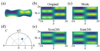
For the solution , the static pattern takes the form of the first line of Eq. (55) and is reflection-symmetric about the -axis. The pattern has an additional symmetry depending on the surface symmetry and combination of eigenfunctions. When both and are even functions on the reflection-symmetric surface, the pattern has symmetry , while when both are odd, it has the symmetry . An example of the latter static pattern is shown in Fig. 6(a) (). On a -periodic surface, when and , the pattern has the symmetry , while when and , it has . An example of the latter static pattern is shown in Fig. 6(b) ().
For other solutions, Eqs. (57) and (58), takes a non-trivial value, and the corresponding propagating patterns have no symmetry. Fig. 6(c) presents an example for the solution of Eq. (57) on a general axisymmetric surface (). Regarding the solution Eq. (58), the parameters are required to satisfy additional conditions, such as , which are unlikely to be achieved.
IV.3 Classification of parallel and helical patterns by steady-state solution of amplitude equations
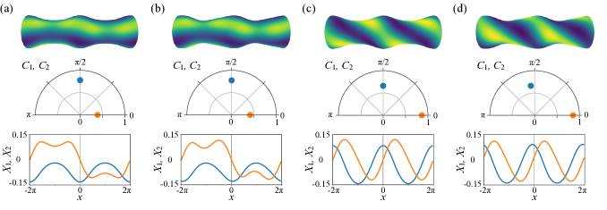
The dynamics of the parallel and helical patterns (Fig. 1) can be understood using the steady-state solutions discussed above. On a -periodic surface along the -axis, parallel patterns are static, whereas helical patterns are static only on a reflection-symmetric surface (Fig. 7 (a)–(c)). These patterns correspond to the steady-state solution in Eq. (52), each consisting of eigenfunctions with characteristic symmetry; for instance, the helical pattern on a reflection-symmetric surface is composed of eigenfunctions with and . The helical pattern begins to move because of the loss of reflection-symmetry [57], which corresponds to the steady-state solution in Eq. (57) of the amplitude equations in Eqs. (21)–(23), where , and the phase difference (Fig. 7(d)).
The parallel static pattern on a -periodic surface along the -axis satisfies and . Because of the loss of the -periodicity of the surface, these relationships no longer hold, and the solution of the amplitude equations becomes Eq. (52), indicating the onset of a propagating wave in a parallel pattern. A numerical example is shown in Fig. 8.
IV.4 Summary of amplitude equations and steady-state solutions
We derived the amplitude equations (18) and (19) for a general axisymmetric surface on which two pairs of modes couple with each other, and the static and propagating patterns correspond to the steady solutions of the amplitude equations. Some coupling terms are eliminated because of the symmetry of the surface (see Eqs. (30) and (31)), which suppresses pattern propagation. The propagation of helical and parallel patterns is caused by the loss of reflection-symmetry and -periodicity, respectively, of the surface along the -axis. For a flat surface, the amplitude equations are reduced to Eqs. (47) and (48), and the pattern is always static. The relationships obtained for the pattern dynamics and the symmetry of the surface and pattern are consistent with those reported in a previous study [57]. In addition, from the amplitude equations, we obtained a non-trivial solution (Eq. (53)) for which the pattern generally has no specific symmetry and propagates. This solution allows the Turing pattern to propagate even on highly symmetric surfaces. A propagating pattern on a sphere was observed in numerical simulation [57].
V Amplitude equation for the Brusselator model
V.1 Reductive perturbation method
The amplitude equations for RDE on axisymmetric curved surfaces can be derived by applying the reductive perturbation method to reaction-diffusion systems in the vicinity of the Turing bifurcation. Consider the general RDE expressed in Eq. (1), for which we explicitly include a bifurcation parameter in the reaction term as . As before, we assume that the equation has a unique uniform steady solution, , satisfying . The uniform solution becomes unstable for , and a Turing pattern occurs.
In the vicinity of the Turing bifurcation at a positive, sufficiently small value of , the amplitude of the pattern, , is expected to be small, and expanding the RDE by and is feasible. The amplitude equations can then be derived from the RDE; see the details of the derivation in Supplemental Text Sec. S2 [68]. In summary, the pattern dynamics of the RDE are approximated by a lower-order expansion with respect to and amplitude , and the pattern dynamics are dominated by the time evolution of :
| (59) | ||||
| (60) |
where and are the first- and higher-order terms in the amplitudes, respectively, and the second equation is referred to as the amplitude equation. These are derived in Eq. (S41) and in Eq. (S42), respectively. The obtained equation (S42) not only validates Eqs. (18) and (19), which are derived as a general form of the amplitude equations, but also determines their coefficients. The simpler forms of amplitude equations (30) and (31) can be understood as follows. As shown in Eqs. (S44)–(S49), the coefficients include integrals of the products of the Laplace–Beltrami eigenfunctions . For example, if the surface is reflection-symmetric about the -axis and and are a pair of even and odd functions, some coefficients are equal to zero owing to the combination of the parity of the eigenfunctions in the integrands, and Eq. (S42) coincides with Eqs. (30) and (31).
V.2 Derivation of Amplitude equation for Brusselator model
We derive the amplitude equations for the Brusselator model in Eqs. (18) and (19) following the general procedure described in Supplemental Text Sec. S2 [68]. We choose the bifurcation parameter , where the reference parameters of the reductive perturbation, , are set such that the growth rates at the two Laplace–Beltrami eigenvalues, and , both become zero. For positive , the pattern can be approximated as
| (61) |
where and are eigenvectors of the linear operator:
| (62) |
Here, are the eigenvalues of the Laplace–Beltrami operator for and are determined from the surface shape. The eigenvalues and parameters satisfy the relation explained in Supplemental Text Sec. S3 [68]. The eigenvectors and their conjugate vectors are expressed by Eqs. (S52) and (S53), respectively. The coefficients of the amplitude equations are then calculated using the products of and , and the integral with respect to . For more details, see Supplemental Text Sec. S3 [68].
V.3 Comparison between Brusselator model and amplitude equations
We numerically solve the amplitude equations derived earlier, and we compare the solution with that of the Brusselator model. In particular, we explore the steady-state solution of the amplitude equations, which corresponds to either a static or propagating pattern, and confirm the claims given in Sec. IV. Dynamics other than the static and propagating patterns are discussed in the next section.
V.3.1 Comparison procedure
The amplitude equations were derived using the following procedure. First, we fixed the surface and selected two pairs of Laplace–Beltrami eigenvalues, and , that were adjacent in the spectral space, and then determined the corresponding eigenfunctions, and . These were chosen to have the same wavenumber . Next, we set the diffusion coefficients and and then determined the model parameters and to satisfy the determinant of to zero (see Eqs. (S58) and (S59)). Subsequently, we set the bifurcation parameter , which was chosen to be sufficiently small and of the order of . The parameters were chosen so that the system would exhibit Turing instability, where the growth rates and were real and positive values. Finally, we determined the coefficients of the amplitude equations, and (), from Eqs. (S43)–(S49), and performed numerical simulations. We also numerically solved the Brusselator model (the original system) using the same surface and parameters.
We compared the solutions obtained from the amplitude equations and the Brusselater model in the phase space of , and phase differences . For the Brusselator model, was obtained by taking the inner product between the pattern and eigenvectors and , where and
| (63) |
where and are the same as the eigenvectors in the amplitude equations.
V.3.2 Comparison of static and propagating patterns
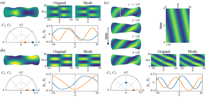
The results of the numerical simulations for the amplitude equations and Brusselator model are summarized in Fig. 9, in which the blue and orange points represent the steady solutions of the amplitude equations and Bursselator model, respectively. Patterns on axisymmetric surfaces and their projection onto the - plane are also shown, where the left panels show the amplitude equations and the right panels show the Brusselator model. The coefficients of the amplitude equations are summarized in Supplemental Table S1 [68].
Figs. 9(a) and (b) show static patterns of the steady solutions. For Fig. 9(a), helical static patterns on the reflection-symmetric and -periodic surface are obtained through the direct simulation of the Brusselator model, while the constructed pattern from the amplitude equations exhibits a similar static pattern with phase difference . For Fig. 9(b), which employs the same parameter set as that in Fig. 6(a), the orbit of the amplitude equations reach a solution similar to that of the corresponding Brusselator model, with phase difference .
Figs. 9(c) and (d) show propagating patterns with phase differences , respectively. For Fig. 9(c), the helical propagating pattern is constructed from the amplitude equations for a surface without reflection-symmetry. slightly deviates from and the pattern is propagating (see also Fig. 10(c)). The patterns and dynamics obtained from the amplitude equations and Brusselator model are in close agreement. For Fig. 9(d), the parameters in Fig. 5(c) are used, where the phase difference is given by the non-trivial solution Eq. (53). We found that pattern dynamics constructed by the amplitude equations are similar to those of the original Brusselator model, indicating that the amplitude equations can capture the non-trivial propagating solution.
V.3.3 Approximation accuracy against bifurcation parameter
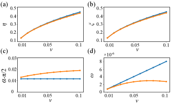
The approximation accuracy against the bifurcation parameters of the helical propagating pattern was evaluated. Under the same conditions as those shown in Fig. 9(c), the bifurcation parameter was changed from to in steps of , resulting in the observation of similar helical patterns. The patterns obtained from the amplitude equations closely approximated those of the Brusselator model, as shown in Figs. 10(a), (b), and (c), in which the amplitudes and and the phase difference of amplitude equations and the original Brusselator model are in close agreement. Figs. 10(a) and (b) confirm that the leading order of the amplitudes is , which is assumed to derive the amplitude equations (Supplemental Text Sec. S2 [68]). The velocities obtained from the amplitude equations and the original Brusselator model are in close agreement (with difference ), and converge as the bifurcation parameter approaches zero (Fig. 10(d)). Consequently, the numerical simulations confirm that the amplitude equations provide a reasonable approximation of the Brusselator model.
VI Pattern dynamics other than propagation
In Sec. III and Sec. V, we derived the amplitude equations for an axisymmetric surface and investigated the steady-state solutions corresponding to the static and propagating patterns. The generic form of the derived equations (Eqs. (18) and (19)) allows us to further explore the possible dynamics, other than propagation, of the RDE on general axisymmetric surfaces; the pattern dynamics are explored by numerically searching for non-stationary solutions of the amplitude equations. In the joint paper [65], we discuss this issue in detail; this section provides a summary of the results. As explained below, our results indicate that the Turing pattern can exhibit oscillatory and chaotic behaviors on curved surfaces.
VI.1 Limit cycle solution and pattern dynamics
We explored the possible pattern dynamics on curved surfaces by conducting numerical searches for amplitude equations (18) and (19). By changing the surface and model parameters of the Brusselator model, the corresponding amplitude equations were derived and numerically solved. For a given parameter set, the derivation of the amplitude equations is the same as that described in Sec. V.3, where we used the surface with and . For an efficient search, the range of the -axis was narrowed.
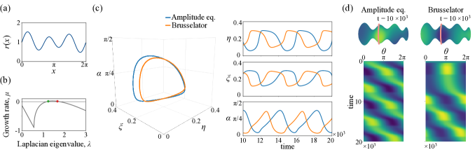
The surface shape and dispersion relations with parameters , , and other surface parameters set to zero are shown in Fig. 11(a) and (b), respectively. We found that the amplitude equations have a limit cycle solution, as represented by the blue line in Fig. 11(c) (see Supplemental Table S1 for the coefficients of the amplitude equations [68]). The corresponding pattern exhibits propagation accompanied by oscillations, as shown in Fig. 11(d) left column. The bifurcation analysis suggests that the oscillatory pattern dynamics appear via Hopf bifurcation from the propagating pattern [65]. We also validated that the original Brusselator model yields similar dynamics (Fig.11(c) orange line and (d) right column). On a flat surface, the pattern remains static as an ordinary Turing pattern. This example demonstrates that the Turing pattern can exhibit more complex dynamics than propagation depending on the surface geometry.
VI.2 Chaotic dynamics in amplitude equations
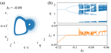
We also searched for complex dynamics by changing the coefficients and () as arbitrarily selectable parameters, with and chosen as real positive values to satisfy the condition of Turing instability. Note that, although this method does not identify the corresponding Brusselator model because of the difficulty in determining surface and model parameters from the coefficients, it allows for a general and efficient investigation of what pattern dynamics are possible. In addition to the limit cycle solution, we observed chaotic dynamics, as shown in Fig. 12. The appearance of the chaotic dynamics can be understood in terms of period-doubling bifurcation against parameter (Fig. 12(b)). The other coefficients of the amplitude equations are listed in Supplemental Table S1 [68]. The existence of such a chaotic solution in the amplitude equations suggests that rich and complex dynamics are possible depending on the geometry of the surface shape. However, the corresponding patterns have not yet been obtained for the Brusselator model on axisymmetric surfaces.
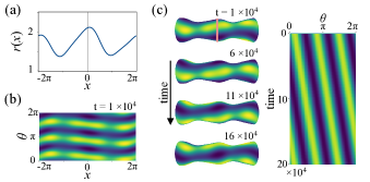
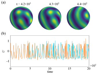
As the search using the amplitude equations is limited to the region near the Turing bifurcation point on axisymmetric surfaces, we examined the Brusselator model under broader conditions. We found an example of chaotic pattern dynamics on a deformed spherical surface, as shown in Fig. 13(a) and [65]. The surface is not axisymmetric and given by a radial function in polar coordinate with . The parameters for the Brusselator model were chosen to be the same as those used in Fig. 2, indicating that the pattern is static on a flat plane. We checked the initial condition sensitivity of the dynamics by comparing two time series of numerical simulations with slightly different initial conditions; the almost identical time series in the early stage eventually become distinguished in the late stage (Fig. 13(b); see details [65]). These results show that chaotic pattern dynamics can arise due to the surface geometry.
VII Discussion
In our previous study, we reported that a Turing pattern that is static on a flat plane can propagate on curved surfaces [57]. Using the relationship in Eq. (7), in which the pattern is assumed to move at a constant speed, we clarified that losses of symmetry in the surface and pattern, such as reflection asymmetry along the -axis of an axisymmetric surface, are required for pattern propagation.
In this study, we performed weakly nonlinear analysis as a complementary approach. This analysis allowed us to explore the generic dynamics of the Turing pattern on curved surfaces near the bifurcation point. The analysis was also advantageous in that the surface and pattern symmetries, which were treated separately in the previous study [57], could be integrated using the eigenfunctions of the Laplace–Beltrami operator, which are determined by the surface shape. Because the mode decomposition of the helical and parallel patterns revealed that static and propagating patterns are described by the two paired modes, we derived the amplitude equations of two complex variables corresponding to the two paired modes. The obtained amplitude equations enabled the classification of pattern dynamics in the vicinity of the Turing bifurcation depending on the symmetry of the pattern and the surface shape. For a general axisymmetric surface, the steady-state solution of the amplitude equations, Eqs. (18) and (19), enables pattern propagation. If a surface has reflection-symmetry or -periodicity along the -axis, the amplitude equations depend on the combination of the modes. For helical and parallel patterns, the amplitude equations drop several terms and are reduced to Eqs. (30) and (31), for which a propagation solution is no longer possible (see below for a nontrivial solution). On a flat plane, the amplitude equations are even simpler (Eqs. (47) and (48)), and the pattern caused by the Turing instability does not move. Overall, the interaction between the modes is more intense on general surfaces and leads to the onset of moving patterns. The propagation conditions given by the relationship between the surface and pattern symmetry are consistent with previous results.
The present study revealed several points beyond previous results. First, we found that the periodicity along the -axis is involved in determining the pattern dynamics. The parallel pattern does not move on the -periodic surface (Fig. 1), whereas the loss of periodicity causes pattern propagation (Fig. 8). Second, the pattern can propagate even on a surface with reflection-symmetry and -periodicity, corresponding to the nontrivial steady-state solution of the amplitude equations. For such a solution, the pattern profile is not symmetric. This type of solution is consistent with the propagating pattern on a sphere determined numerically in the previous study [57]. Third, a weakly nonlinear analysis revealed that patterns on axisymmetric surfaces exhibited more complex dynamics than propagation, including oscillating and chaotic chemical waves. Some of these dynamics were confirmed through numerical simulations of the RDE for the Brusselator model (Fig. 11). In particular, motivated by the chaotic solutions in the amplitude equations, we found a chaotic Turing pattern by direct numerical simulation of Brusselator model on a deformed spherical surface (see the joint paper [65]). These findings provide a new perspective on the intricate interplay between surface characteristics and pattern dynamics.
The present study should be extended to pattern dynamics on general surfaces without axisymmetry, for which weakly nonlinear analysis is applicable. By performing numerical simulations of the RDE on several surfaces, we observed chaotic patterns (Fig. 13) and moving patterns with varying speeds (see Movie 2 [68]). Here, we briefly consider these patterns in terms of the amplitude equations: without axisymmetry (i.e., no translational invariance along the -axis), amplitude equations can have quadratic terms representing additional interactions among modes, and more complex dynamics could arise. A detailed analysis is required in the future.
Pattern dynamics driven by surface curvature are applicable to natural and engineering systems. By controlling the parameters of the surfaces and reactions, the pattern can be switched between oscillating, static, and propagating states. In biological systems, such dynamics can be used for information transduction, guidance of cellular migration, and positioning of molecular localization. Analyses using amplitude equations are useful for predicting pattern dynamics and can also provide a basis for the engineering of patterns on curved surfaces. In the future, analysis of the stability and bifurcation of the amplitude equations will further improve our understanding of pattern dynamics on general curved surfaces, and will also be useful for dynamics in network systems [72, 73], and on deformable surfaces [74, 75, 76].
Acknowledgements
This study was supported by
JST SPRING JPMJSP2108 (to R.N.),
JSPS KAKENHI JP23KJ0641 (to R.N.),
JPJSJPR 20191501 (to S.I.),
and JST CREST JPMJCR1923, Japan (to S.I.).
Author contributions
R.N. and S.I. both proposed the research direction, contributed to the theoretical analysis,
and wrote the manuscript. R.N. performed all numerical simulations.
References
- [1] Y. Fuseya, H. Katsuno, K. Behnia and A. Kapitulnik, Nanoscale Turing patterns in a bismuth monolayer, Nature Physics , 1031-1036 (2021).
- [2] T. Aasba, L. Peng, T. Ono, S. Akutagawa, I. Tanaka, H. Murayama, S. Suetsugu, A. Razpopov, Y. Kasahara, T. Terashima et al., Growth of self-integrated atomic quantum wires and junctions of a Mott semiconductor, Science Advances , 173-179 (2023).
- [3] J. Ross, S. C. Müller, and C. Vidal, Chemical waves, Science , 460 (1988).
- [4] J. D. Murray, Mathematical Biology I: An Introduction Vol. 3., (Springer, New York, 2002), J. D. Murray, Mathematical biology II: Spatial models and biomedical applications. Vol. 3., (Springer, New York, 2003).
- [5] L. Manukyan, S. A. Montandon, A. Fofonjka, S. Smirnov and M. C. Milinkovitch, A living mesoscopic cellular automaton made of skin scales, Nature , 173-179 (2017).
- [6] C. E. Tarnita, J. A. Bonachela, E. Sheffer, J. A. Guyton, T. C. Coverdale, R. A. Long and R. M. Pringle, A theoretical foundation for multi-scale regular vegetation patterns, Nature , 398-401 (2017).
- [7] R. Goyal, M. Jucker, A. Sen Gupta, H. H. Hendon, and M. H. England, Zonal wave 3 pattern in the southern hemisphere generated by tropical convection, Nat. Geosci. , 732 (2021).
- [8] A. Radja, E. M. Horsley, M. O. Lavrentovich, and A. M. Sweeney, Pollen cell wall patterns form from modulated phases, Cell , 856 (2019).
- [9] S. Alonso, M. Bär, and B. Echebarria, Nonlinear physics of electrical wave propagation in the heart: a review, Rep. Prog. Phys. , 096601 (2016).
- [10] J. Bischof, C. A. Brand, K. Somogyi, I. Májer, S. Thome, M. Mori, U. S. Schwarz, and P. Lénárt, A cdk1 gradient guides surface contraction waves in oocytes, Nat. Commun. , 1-10 (2017).
- [11] L. Wettmann and K. Kruse, The Min-protein oscillations in Escherichia Coli: an example of self-organized cellular protein waves, Philos. Trans. R. Soc. Lond. B Biol. Sci. , (2018).
- [12] T. H. Tan, J. Liu, P. W. Miller, M. Tekant, J. Dunkel, and N. Fakhri, Topological turbulence in the membrane of a living cell, Nat. Phys. , 657-662 (2020).
- [13] N. Saito, and S. Sawai, Three-dimensional morphodynamic simulations of macropinocytic cups, iScience , 103087 (2021).
- [14] M. K. McGuire, C. A. Fuller, J. F. Lindner, and N. Manz, Geographic tongue as a reaction-diffusion system, Chaos , 033118 (2021).
- [15] Y. Maroudas-Sacks, L. Garion, L. Shani-Zerbib, A. Livshits, E. Braun, and K. Keren, Topological defects in the nematic order of actin fibres as organization centres of Hydra morphogenesis, Nat. Phys. , 251-259 (2021).
- [16] D. Baptista, L. Teixeira, C. van Blitterswijk, S. Giselbrecht, and R. Truckenmüller, Overlooked? underestimated? effects of substrate curvature on cell behavior, Trends Biotechnol. , 838 (2019).
- [17] S. Ehrig, B. Schamberger, C. M. Bidan, A. West, C. Jacobi, K. Lam, P. Kollmannsberger, A. Petersen, P. Tomancak, K. Kommareddy et al., Surface tension determines tissue shape and growth kinetics, Sci. Adv., , eaav9394 (2019).
- [18] B. Schamberger, R. Ziege, K. Anselme, M. B. Amar, M. Bykowski, A. P. G. Castro, A. Cipitria, R. A. Coles, R. Dimova, M. Eder et al., Curvature in biological systems: Its quantification, emergence, and implications across the scales, Adv. Mater., , e2206110 (2023).
- [19] B. Antony, Mechanisms of membrane curvature sensing, Annu. Rev. Biochem. , 101-123 (2011).
- [20] M. Simunovic, G. A. Voth, A. Callan-Jones, and P. Bassereau, When physics takes over: BAR proteins and membrane curvature, Trends Cell Biol. , 780 (2015).
- [21] S. Yang, X. Miao, S. Arnold, B. Li, A. T. Ly, H. Wang, M. Wang, X. Guo, M. M. Pathak, W. Zhao et al., Membrane curvature governs the distribution of Piezo1 in live cells, Nat. Commun. , 7467 (2022).
- [22] L. Pieuchot, J. Marteau, A. Guignandon, T. Dos Santos, I. Brigaud, P. F. Chauvy, T. Cloatre, A. Ponche, T. Petithory, P. Rougerie et al., Curvotaxis directs cell migration through cell-scale curvature landscapes, Nat. Commun. , 1-13 (2018).
- [23] M. Luciano, S.-L. Xue, W. H. De Vos, L. Redondo-Morata, M. Surin, F. Lafont, E. Hannezo, and S. Gabriele, Cell monolayers sense curvature by exploiting active mechanics and nuclear mechanoadaptation, Nature Physics, , 1382-1390 (2021).
- [24] K. Horibe, K. Hironaka, K. Matsushita, and K. Fujimoto, Curved surface geometry-induced topological change of an excitable planar wavefront, Chaos , 093120 (2019).
- [25] V. A. Davydov, V. G. Morozov, and N. V. Davydov, Ring-shaped autowaves on curved surfaces, Phys. Lett. A , 326-330 (2000).
- [26] J. Gomatam and F. Amdjadi, Reaction-Diffusion Equations on a Sphere: Meandering of Spiral Waves, Phys. Rev. E , 3913 (1997).
- [27] H. Yagisita, M. Mimura, and M. Yamada, Spiral wave behaviors in an excitable reaction-diffusion system on a sphere, Physica D , 126 (1998).
- [28] V. A. Davydov, V. G. Morozov, and N. V. Davydov, Critical properties of autowaves propagating on deformed cylindrical surfaces, Phys. Lett. A , 265 (2003).
- [29] F. Kneer, E. Schöll, and M. A. Dahlem, Nucleation of reaction-diffusion waves on curved surfaces, New J. Phys. , 053010 (2014).
- [30] S. Białecki, P. Nałecz-Jawecki, B. Kaźmierczak, and T. Lipniacki, Traveling and standing fronts on curved surfaces, Physica D , 132215 (2020).
- [31] L. R. Gómez, N. A. García, V. Vitelli, J. Lorenzana, and D. A. Vega, Phase nucleation in curved space, Nat. Commun. , 6856 (2015).
- [32] A. R. Singh, T. Leadbetter, and B. A. Camley, Sensing the shape of a cell with reaction diffusion and energy minimization, Proc. Natl. Acad. Sci. U. S. A. , e2121302119 (2022).
- [33] B. Q. Ai, W. J. Zhu, and J. J. Liao, Collective transport of polar active particles on the surface of a corrugated tube, New J. Phys. , 093041 (2019).
- [34] J. P. Brasselet, J. Seade, and T. Suwa, Vector fields on singular varieties (Springer Science & Business Media, 2009).
- [35] S. Kralj, R. Rosso, and E. G. Virga, Curvature control of valence on nematic shells, Soft Matter , 670-683 (2011).
- [36] L. N. Carenza, G. Gonnella, D. Marenduzzo, G. Negro, and E. Orlandini, Cholesteric Shells: Two-Dimensional Blue Fog and Finite Quasicrystals, Phys. Rev. Lett. , 027801 (2022).
- [37] S. Shankar, M. J. Bowick, and M. C. Marchetti, Topological sound and flocking on curved surfaces, Phys. Rev. X , 031039 (2017).
- [38] F. C. Keber, E. Loiseau, T. Sanchez, S. J. Decamp, L. Giomi, M. J. Bowick, M. C. Marchetti, Z. Dogic, and A. R. Bausch, Topology and dynamics of active nematic vesicles, Science , 1135-1139 (2014).
- [39] A. M. Turing, The chemical basis of morphogenesis, Phil. Trans. R. Soc. Lond. B , 37-72 (1952).
- [40] S. Kondo, and T. Miura, Reaction-diffusion model as a framework for understanding biological pattern formation, Science , 1616-1620 (2010).
- [41] J. Raspopovic, L. Marcon, L. Russo, and J. Sharpe, Digit patterning is controlled by a Bmp-Sox9-Wnt Turing network modulated by morphogen gradients, Science , 566-570 (2014).
- [42] S. Ishihara, and K. Kaneko, Turing pattern with proportion preservation, J. Theor. Biol. , 683-693 (2006).
- [43] R. G. Plaza, F. Sánchez-Garduño, P. Padilla, R. A. Barrio, and P. K. Maini, The effect of growth and curvature on pattern formation, J. Dyn. Differ. Equ. , 1093-1121 (2004).
- [44] V. Giulio, M. Davide, B. G. Andrew, and O. Enzo, Curvature-driven positioning of Turing patterns in phase-separating curved membranes, Soft Matter , 3888-3896 (2016).
- [45] A. L. Krause, E. A. Gaffney, P. K. Maini, and V. Klika, Modern perspectives on near-equilibrium analysis of Turing systems, Phil. Trans. R. Soc. A. , 20200268 (2021).
- [46] L. Charette, Pattern formation on curved surfaces, Ph.D. Thesis, The University of British Columbia, Canada, (2019).
- [47] C. Varea, J. L. Aragon, and R. A. Barrio, Turing patterns on a sphere, Phys. Rev. E , 4588 (1999).
- [48] P. C. Matthews, Pattern formation on a sphere, Phys. Rev. E , 036206 (2003).
- [49] M. Núñez-López, G. Chacón-Acosta, and J. A. Santiago, Diffusion-driven instability on a curved surface: spherical case revisited, Braz. J. Phys. , 231-238 (2017).
- [50] D. Lacitignola, B. Bozzini, M. Frittelli, and I. Sgura, Turing pattern formation on the sphere for a morphochemical reaction-diffusion model for electrodeposition, Commun. Nonlinear Sci. Numer. Simul. , 484-508 (2017).
- [51] F. Sánchez-Garduno, A. L. Krause, J. A. Castillo, and P. Padilla, Turing-Hopf patterns on growing domains: the torus and the sphere, J. Theor. Biol. , 136-150 (2019).
- [52] S. S. Liaw, C. C. Yang, R. T. Liu, and J. T. Hong Turing model for the patterns of lady beetles, Phys. Rev. E , 041909 (2001).
- [53] W. Nagata, H. R. Z. Zangeneh, and D. M. Holloway, Reaction-diffusion patterns in plant tip morphogenesis: bifurcations on spherical caps, Bull. Math. Biol. , 2346-2371 (2013).
- [54] S. Nampoothiri, and A. Medhi, Role of curvature and domain shape on Turing patterns, arXiv:1705.02119 (2017).
- [55] S. Nampoothiri, Effect of geometry on the positioning of a single spot in reaction–diffusion systems, arXiv:1909.06528 (2019).
- [56] J. R. Frank, J. Guven, M. Kardar, and H. Shackleton, Pinning of diffusional patterns by non-uniform curvature, EPL , 48001 (2019).
- [57] R. Nishide, and S. Ishihara, Pattern Propagation Driven by Surface Curvature, Phys. Rev. Lett. , 224101 (2022).
- [58] G. Nicolis, and I. Prigogine, Self–organization in nonequilibrium systems (Wiley, New York, 1977).
- [59] B. Peña and C. Pérez-García, Stability of Turing Patterns in the Brusselator Model, Phys. Rev. E , 056213 (2001).
- [60] I. Lengyel, and I. R. Epstein, Modeling of Turing structures in the chlorite-iodide-malonic acid-starch reaction system, Science , 650-652 (1991).
- [61] T. Bánsaǵi Jr., and A. F. Taylor, Helical Turing patterns in the Lengyel-Epstein model in thin cylindrical layers, Chaos , 064308 (2015).
- [62] M. C. Cross and P. C. Hohenberg, Pattern formation outside of equilibrium, Rev. Mod. Phys. , 851 (1993).
- [63] R. Hoyle, Pattern formation: An introduction to methods (Cambridge University Press, 2006).
- [64] Y. Kuramoto, Chemical oscillations, waves, and turbulence (Springer Science & Business Media, 2012).
- [65] R. Nishide, and S. Ishihara, Oscillatory and chaotic pattern dynamics driven by surface curvature.
- [66] A. K. M. Nazimuddin, M. H. Kabir, and M. O. Gani, Oscillatory wave patterns and spiral breakup in the Brusselator model using numerical bifurcation analysis, J. Comput. Sci. , 101720 (2022).
- [67] A. L. Krause, M. A. Ellis, and R. A. Van Gorder, Influence of curvature, growth, and anisotropy on the evolution of Turing patterns on growing manifolds, Bull. Math. Biol. , 759-799 (2019).
- [68] Supplemental Material.
- [69] G. Xu, Discrete Laplace–Beltrami operator on sphere and optimal spherical triangulations, Int. J. Comput. Geom. Appl. , 75-93 (2006).
- [70] J. Porter and E. Knobloch, Complex dynamics in the 1:3 spatial resonance, Physica D , 138 (2000).
- [71] C. Kittel and P. McEuen, Introduction to solid state physics (John Wiley & Sons, 2018).
- [72] H. Nakao, and A. S. Mikhailov, Turing patterns in network-organized activator-inhibitor systems, Nat. Phys. , 544-550 (2010).
- [73] J. van der Kolk, G. García-Pérez, N. E. Kouvaris, M. Á. Serrano, and M. Boguñá, Emergence of Geometric Turing Patterns in Complex Networks, Phys. Rev. X , 021038 (2023).
- [74] G. Toole and M. K. Hurdal, Turing models of cortical folding on exponentially and logistically growing domains, Comput. Math. Appl. , 1627 (2013).
- [75] P. W. Miller, N. Stoop, and J. Dunkel, Geometry of wave propagation on active deformable surfaces, Phys. Rev. Lett. , 268001 (2018).
- [76] N. Tamemoto, and H. Noguchi, Pattern formation in reaction-diffusion system on membrane with mechanochemical feedback, Sci. Rep. , 19582 (2020).