Geometric Constraints in Deep Learning Frameworks: A Survey

Abstract

Stereophotogrammetry is an emerging technique of scene understanding. Its origins go back to at least the 1800s when people first started to investigate using photographs to measure the physical properties of the world. Since then, thousands of approaches have been explored. The classic geometric techniques of Shape from Stereo is built on using geometry to define constraints on scene and camera geometry and then solving the non-linear systems of equations. More recent work has taken an entirely different approach, using end-to-end deep learning without any attempt to explicitly model the geometry. In this survey, we explore the overlap for geometric-based and deep learning-based frameworks. We compare and contrast geometry enforcing constraints integrated into a deep learning framework for depth estimation or other closely related problems. We present a new taxonomy for prevalent geometry enforcing constraints used in modern deep learning frameworks. We also present insightful observations and potential future research directions.

Keywords Depth Estimation  $\cdot$ Monocular  $\cdot$ Stereo  $\cdot$ Multi-view Stereo  $\cdot$ Geometric Constraints  $\cdot$ Stereophotogrammetry  $\cdot$ Scene understanding  $\cdot$ self-supervised Depth Estimation  $\cdot$ Photometric Consistency  $\cdot$ Smoothness  $\cdot$ Geometric Representations  $\cdot$ Structural Consistency

1 Introduction

Figure 1: Overview of geometric constraints concepts covered in the survey paper. We discuss geometric constraints used in deep learning-based depth estimation and other closely related frameworks.

Traditional stereo or multi-view stereo (MVS) depth estimation methods rely on solving for photometric and geometric consistency constraints across view(s) for consistent depth estimation [1, 2, 3, 4, 5, 6, 7, 8]. With the phenomenal rise of deep learning frameworks [9], like Convolutional neural networks (CNNs) [10], Recurrent neural networks (RNNs) [11], and Vision transformers (ViTs) [12], which can extract deep local and high-level features, the the requirement to apply photometric and geometric consistency constraints has significantly reduced, especially in supervised depth estimation methods. Deeper features significantly improved feature matching leading to a huge improvement in depth estimates [13, 14, 15, 16]. The application of geometric constraints remains limited to the use of plane-sweep algorithm [17] form majority of supervised stereo and MVS methods.

In a typical supervised stereo or MVS depth estimation framework, the plane-sweep algorithm is applied to create a matching (cost) volume, which is then aggregated based on a metric. The aggregated volume – cost volume, is then regularized using 3D-CNNs or RNNs to produce a coherent estimate. The lack of ground truth in unsupervised/self-supervised depth estimation methods do not allow such freedom. Photometric and geometric consistency constraints remain a key part of unsupervised frameworks [18, 19, 20, 21, 22]. Some of the other closely related problems, like structure from motion [23, 24], video-depth estimation [25, 26], semantic-segmentation [27, 28, 29, 18], and monocular depth estimation [30, 31], also apply various geometric constraints for a consistent result. In this survey, we focus on all such methods that integrate photometric or geometric constraints in deep learning-based frameworks and are closely related to depth estimation problem. Fig. 1 shows the collection of such geometric constraints and their associated problems, that are covered in this survey. We discuss the theory and mathematical formulation of all these concepts and present a carefully crafted taxonomy, see Fig. 2.

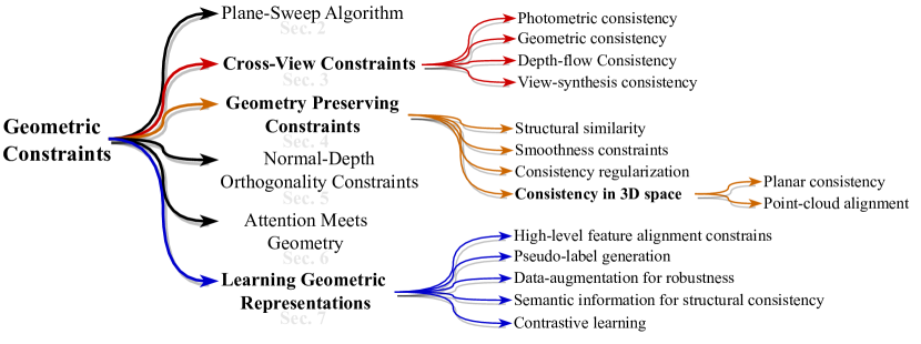
Figure 2: Our taxonomy of current geometric constraints used in deep learning-based depth estimation and closely related frameworks.

Throughout this paper, we keep our focus on geometry-enforcing concepts used across different problems that either do depth estimation or are closely related to depth estimation problems. We only discuss the specific concepts used and their relevance to stereo or MVS depth estimation frameworks. This survey is organized in $8$ sections. Starting from Sec. 2, we discuss the broad classification of geometric constraints presented in our taxonomy show in Fig. 2. For most of the sections, we first describe the a most common mathematical formulation of the concept that covers the majority of the methods and then, we describe different modifications applied to it by specific methods. Sec. 2 describes the traditional plane sweep algorithm and its variants. Sec. 3 focuses on all such geometric constraints that use alternate view(s) for enforcing consistency (cross-view consistency). Sec. 4 delves into geometric constraints that enforce structural consistency between a reference image and a target image to preserve the structural integrity of the scenes. Sec. 5 focuses on the orthogonal relation between depth and surface normal to guide geometric consistency. Sec. 6 discusses the integration of geometric constraints in attention mechanism and Sec. 7 presents the methods to enforce geometry-based representation learning in deep neural networks. We present our conclusion in Sec. 8.

2 Plane Sweep Algorithm

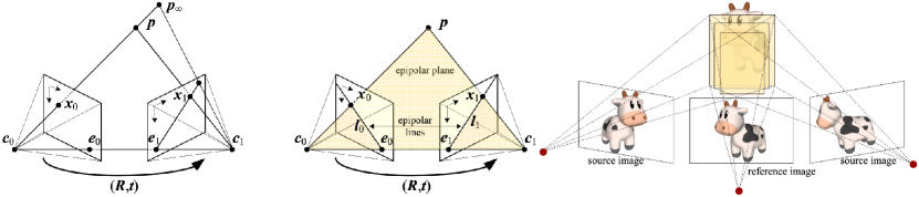
Figure 3: Epipolar geometry, Left: epipolar line segment corresponding to one ray (Fig. reused from [8]), Center: corresponding set of epipolar lines and their epipolar plane (Fig. reused from [8]), $R$, $t$ are the rotation and translation parameters, and $l_{i}$ is the epipolar line segment. Right: illustration of plane-sweep algorithm (Fig. reused from[32])

Stereophotogrammetry is the process of estimating the 3D coordinates of points on an object by utilizing measurements from two or more images of the object taken from different positions [33]. This involves stereo matching where two or more images are used to find matching pixels in the images and convert their 2D positions into 3D depths [8]. The process of finding matching pixels is based on the geometry of stereo matching (epipolar geometry), i.e the process of computing the range of possible locations of a pixel from an image that might appear in another image. In this section, first, we discuss the epipolar geometry for two rectified images and then describe a general resampling algorithm , plane sweep, that can be used to perform multi-image stereo matching with arbitrary camera configuration.

Fig. 3 (left) shows the epipolar constraints of how a pixel in one image $x_{0}$ projects to an epipolar line segment in the other image. The line segment is bounded by $p_{\infty}$ – projection of the original viewing ray, and $c_{0}$ – projection of the original camera center into the second camera, called epipole $e_{1}$. The projections of the epipolar line in the second image back into the first image give us another line segment bounded by corresponding epipole $e_{0}$. Extension of these two line segments to infinity gives us a pair of corresponding epipolar lines, Fig. 3(center), that are the intersection of the two image planes, epipolar planes, that passes through both camera centers $c_{0}$ and $c_{1}$. $p$ is the point of interest [6, 7].

Multi-image stereo reconstruction is a process to recover the 3D scene structure from multiple overlapping images with known intrinsic ($K$) and extrinsic ($E$) camera parameters [17]. More precisely, source images are projected to fronto-parallel planes of the reference camera frustum, and the photoconsistency of these images is analyzed, see Fig. 3 (right). This process is commonly known as plane-sweep approach [17, 34, 35, 32]

The plane-sweep method is based on the premise that areas of space where several image features viewing rays intersect are likely to be the 3D location of observed scene features. In this method, a single plane partitioned into cells is swept through the volume of space along a line perpendicular to the plane [17], perpendicular to reference camera frustum as shown in Fig. 3 (right). At each position of the plane along the sweeping path, the number of intersecting viewing rays is tallied. This is done by back-projecting features from each source image onto the sweeping plane and noting the features that fall within some threshold of back-projected point position. Cells with the largest tallies are hypothesized as the location of 3D scene features, corresponding depth hypothesis in the case of depth maps, are selected [32, 17].

The plane-sweep method can directly estimate the disparity (for stereo) or depth values (for MVS), but modern deep learning-based frameworks use it to create matching volume corresponding to each source image and the reference image. The matching volume is aggregated based on a metric to create a cost volume. The cost volume is then regularized either by 3D-CNNs [13, 14, 16, 15] or by RNNs [36, 37]. The metric used for cost volume aggregation can vary from method to method. For example, Huang et al. [38] compute pairwise matching costs between a reference image and neighboring source images and fuse them with max-pooling. MVSNet [13], R-MVSNet [36] and CasMVSNet [14] computes the variance between all encoded features warped onto each sweep plane and regularizes it with 3D-U-Net [39]. TransMVSNet [15] computes similarity-based cost volume for regularization. Yang et al. [40] reuse cost volume from the previous stage, along with the partial cost volume of the current stage in the multi-stage MVS framework. They create a pyramidal structure in cost volume creation.

Plane sweeping typically assumes surfaces to be fronto-parallel, which causes ambiguity in matching where slanted surfaces are involved like urban scenes [41]. Gallup et al. [41] propose to perform multiple plane sweeps, where each plane sweep is intended to take care of planar surfaces with a particular normal. The proposed method is applied in three steps, first, the surface normals of the ground and facade planes are identified by analyzing their 3D points obtained through the sparse structure from motion. Then, a plane sweep for each surface normal is applied, resulting in multiple depth hypotheses for each pixel in the final depth map. Finally, the best depth/normal combination for each pixel is selected based on a cost or by multi-label graph cut method [5, 42, 43].

3 Cross-View Constraints

Cross-view constraints are applied to a scene with more than one view. It can be applied to stereo (two views per scene) and MVS ($N>2$ view per scene) frameworks by projecting one view, either reference or source view, to the other view or vice-versa. Once projected to the other view, various constraints, like, photometric consistency, depth flow consistency, and view synthesis consistency can be utilized. An alternate way of utilizing cross-view constraints is to use forward-backward reprojection, where one view is projected to the other view and then it is back-projected to the first view to check the geometrical consistency of the scene. In this section, we discuss all such approaches that use cross-view consistency constraints in end-to-end deep learning-based frameworks.

3.1 Photometric Consistency

Photometric consistency minimizes the difference between a real image and a synthesized image from other views. The real and the synthesized images are denoted as reference ($I_{ref}$) and source ($I_{src}$) views in MVS, left ($I_{L}$) and right ($I_{R}$) or vice-versa in stereo problems. For video depth estimation, next frame ($I_{+}$) is compared with the current frame ($I_{0}$). The synthesized images are warped into real image views using intrinsic ($K$) and extrinsic ($E$) parameters. The warping process brings both real and synthesized images in the same camera view. The photometric loss is calculated as per Eqs. 1- 3. Here, we use notations related to MVS problem formulation.

Two main variations of photometric loss are, pixel photometric loss and gradient photometric loss. As the name suggests, pixel photometric loss is the comparison between pixel values of these images, and gradient photometric loss is the comparison of the gradients of these images. Sometimes, pixel photometric loss and gradient photometric loss are combined for a more robust form of photometric loss, called robust photometric loss. Eqs. 1, 2 and 3 shows the pixel, gradient, and robust formulation of photometric loss for MVS methods.

$$\mathcal{L}_{photo_{pixel}} =\frac{||(I_{ref}-\hat{I}_{src\rightarrow ref})\odot M||_{l_{i}}}{||M||_{1}}$$ (1)

$$\mathcal{L}_{photo_{grad}} =\frac{||(\triangledown I_{ref}-\triangledown\hat{I}_{src\rightarrow ref})\odot M||_{l_{i}}}{||M||_{1}}$$ (2)

$$\mathcal{L}_{photo_{robust}} =\lambda_{1}.\mathcal{L}_{photo_{pixel}}+\lambda_{2}.\mathcal{L}_{photo_{grad}}$$ (3)

where, $l_{i}$ denotes $L_{1}$ or $L_{2}$ norm, $M$ denotes the mask, and $\lambda_{1},\lambda_{2}$ denotes scaling factor for pixel and gradient photometric losses, respectively. $\odot$ denotes pixel-wise multiplication.

There can be different ways of formulating Eqs 1, 2 and 3 based on the choice of view to be warped. Most methods [44, 45, 46, 22, 47, 48] warp source views to the reference view called source-reference warp, as shown in Eqs 1, 2 and 3. But some methods warp the reference view to source views (reference-source warp) for estimating the photometric loss [49], replace src with ref and vice-versa in Eqs 1, 2 and 3 to generate such a formulation. Other methods like, [50] use patch-wise photometric consistency to estimate the photometric loss. We highlight all such variations of photometric consistency formulation in the next few paragraphs.

We start with pixel photometric loss and its variations. Mallick et al. [44] use pixel formulation of photometric loss between reference and source views to enforce geometric consistency in adaptive learning approach for self-supervised MVS pipeline. Zhao et al. [45] use a similar formulation of pixel photometric loss in self-supervised monocular depth estimation problem to promote cross-view geometric consistency. Xu et al. [51] use a slightly different formulation of pixel photometric loss based on the condition that a pixel in one view finds a valid pixel in another view for semi-supervised MVS pipeline. The following equation represents this formulation

$$\mathcal{L}_{photo_{pixel}}=\frac{\Phi(1\leq\hat{p}_{i}\leq[H,W])||I_{ref}(p_{i})-\hat{I}_{src\rightarrow ref}(p_{i})||_{L_{2}}}{\Phi(1\leq\hat{p}_{i}\leq[H,W])}$$ (4)

where, $p_{i}$ denotes each pixel, $\Phi(1\leq\hat{p}_{i}\leq[H,W])$ indicates whether the current pixels $p_{i}$ can find a valid pixel $\hat{p}_{i}$ in other source view. $H,W$ denotes the height and width of the image, respectively.

Li et al. [49] use a slightly different formulation of pixel photometric loss by warping reference view to source views, instead of warping source view to the reference view, to calculate the $L_{1}$ distance between reference-source depth maps.

$$\mathcal{L}_{photo_{pixel}}=\frac{1}{N-1}\sum^{N}_{i=1}|I_{src_{i}}-\hat{I}_{ref\rightarrow src_{i}}|$$ (5)

where $N$ is the total number of source views.

All the above-mentioned methods use pixel-wise warping operations to estimate photometric error. Yu et al. [52] propose patch-based warping of the extracted key points. It uses the point selection strategy from Direct Sparse Odometry (DSO) [53] and defines a support domain $\Omega(P_{i})$ over each point $P_{i}$’s local window. The photometric error is then estimated over each support domain $\Omega(P_{i})$, instead of a single point. It is called patch photometric consistency. Dong and Yao [50] applied a similar approach to estimate patch photometric error. Unlike [52], which uses DSO to extract key points, it uses each pixel as a key point. It defines a $m^{2}$ sized square patch centering on the pixel $P$ as $\Omega(P)$. The local patch $\Omega(P)$ is small so that it can be treated as a plane [52] and it assumes that the patch shares the same depth as the center pixel. This patch is warped from the source view to the reference view and $L_{1}$ difference between pixel values is estimated as $\mathcal{L}_{photo_{patch}}$, given as

$$\mathcal{L}_{photo_{patch}}=\frac{1}{N-1}\sum^{N}_{i=1}|I_{ref}-\hat{I}_{src\rightarrow ref}|\odot M_{ref}$$ (6)

where $N$ indicates the number of source views and $M_{ref}$ indicates the reference view mask. $\odot$ denotes element-wise multiplication operation.

While pixel photometric consistency is significantly used to achieve better geometric consistency across views, their performance is susceptible to changes in lighting conditions. Change in lighting conditions makes enforcing pixel-level consistency difficult, but image gradients are more invariant to such changes. Many methods employ gradient photometric loss alongside pixel photometric loss. Since the addition of the gradient term makes the photometric loss more robust, it is called robust photometric loss. MVS methods like [46, 22, 47, 48, 18] use this formulation, Eq. 3, during end-to-end training. $\lambda_{1}$ and $\lambda_{2}$ are the tunable hyper-parameters in Eq. 3.

While most mentioned MVS methods use asymmetric pipeline – estimating only the reference depth map using both the reference and source RGB images, Dai et al. [54] use a symmetric pipeline for MVS, i.e. the network predicts depth maps of all views simultaneously. With $N$ depth estimates, one per view, the method uses a bidirectional calculation of photometric consistency between each pair of views, called cross-view consistency loss. They do not use robust formulations for cross-view consistency.

3.2 Geometric Consistency

Just like photometric consistency, geometric consistency also involves cross-view consistency checks with projections. For photometric consistency, one view, either reference or source, is warped to another view to calculate the consistency error. Geometric consistency employ forward-backward reprojection (FBR) to estimate the error. FBR involves a series of projections of the reference view to estimate the geometric error, see Alg. 1. First, we project the reference image ($I_{r}$) to the source view ($I_{r\rightarrow s}$), then, we remap the projected reference view $I_{r\rightarrow s}$ to generate $I_{s_{remap}}$ and finally, we back-project $I_{s_{remap}}$ to the reference view to obtain $I_{r\rightleftarrows s}$. $I_{r\rightleftarrows s}$ is then compared with original $I_{r}$ to estimate the photometric error.

Inputs: $I_{r},c_{s},I_{s},c_{s}$

$K_{r},E_{r}\leftarrow c_{r}$; $K_{s},E_{s}\leftarrow c_{s}$

$I_{(r\rightarrow s)}\leftarrow K_{s}\cdot E_{s}\cdot E_{r}^{-1}\cdot K_{r}^{-1}\cdot I_{r}$ $\triangleright$ Project

$X_{I_{(r\rightarrow s)}},Y_{I_{(r\rightarrow s)}}\leftarrow I_{(r\rightarrow s)}$

$I_{s_{remap}}\leftarrow REMAP(I_{s},X_{I_{(r\rightarrow s)}},Y_{I_{(r\rightarrow s)}})$ $\triangleright$ Remap

$I_{r\rightleftarrows s}\leftarrow K_{r}\cdot E_{r}\cdot E_{s}^{-1}\cdot K_{s}^{-1}\cdot I_{s_{remap}}$ $\triangleright$ Back project

Algorithm 1 Forward Backward Reprojection (FBR)

Dong and Yao [50] use cross-view geometric consistency by applying FBR in the pixel domain in an unsupervised MVS pipeline. Once the FBR steps are done, the actual pixel values between the original reference image $I_{r}$ and back-projected reference images $I_{r\rightleftarrows s}$ are used to check the geometrical consistency of the depth estimates. It diminishes the matching ambiguity between reference and source views. The following equation shows its mathematical formulation

$$\mathcal{L}_{geometric}=\frac{1}{N}\sum^{N}_{i=1}|I_{ref}-\hat{I}^{i}_{ref\rightleftarrows src}|\odot M_{ref}$$ (7)

where $N$ indicates the number of source views and $M_{ref}$ denotes the reference view mask. $\odot$ is the element-wise multiplication operation. Sometimes,

The Geometric consistency can be extended to the 3D coordinates of the camera using the concept of back-projection [55, 23]. Chen et al. [23] apply this modified geometric consistency in 3D space for a video depth estimation problem, called 3D geometric consistency. For a given source image pixel $P_{src}$ and corresponding reference image pixel $P_{ref}$, their 3D coordinates are obtained by back projection. The inconsistency between the estimates of the same 3D point is then estimated and used as a penalty. The loss value represents the 3D discrepancy of predictions from two views. [55] use a similar formulation to overcome the deficiencies of photometric loss in a self-supervised monocular depth estimation framework.

3.3 Cross-View Depth-Flow Consistency

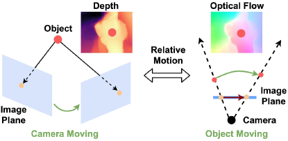
Figure 4: Intuition of Depth2Flow module. The relative motion of moving camera can be viewed as a moving object with a still camera to estimate optical flow. Figure reused from [46]

Depth-flow estimations are typically used in optical flow problems [56, 57]. But it can easily be adapted in MVS problems by estimating flow from estimated depth maps as well as from input RGB images and comparing them. Xu et al. [46] propose a novel flow-depth consistency loss to regularize the ambiguous supervision in the foreground of depth maps. Estimation of flow-depth consistency loss requires two modules for an MVS method, RGB2Flow and Depth2Flow. As the name suggests, the Depth2Flow module transforms the estimated depth maps to virtual optical flow between the reference and arbitrary source view and the RGB2Flow module uses [56] to predict the optical flow from the corresponding reference-source pairs. The two flows predicted should be consistent with each other.

Depth2Flow module

In an MVS system, cameras move around the object to collect multi-view images. If we consider the relative motion between the object and the camera, the camera can be assumed to be fixed and the object can be assumed to be in motion towards the virtually still camera, see Fig. 4. This virtual motion can be represented as a dense 3D optical flow and it should be consistent with the 3D correspondence in real MVS systems. The virtual flow for a pixel $p_{i}$ can be defined as

$$\hat{F}_{r\rightarrow s}=Norm[K_{s}.E_{s}(K_{r}.T_{r})^{-1}I_{r}(p_{i})]-p_{i}$$ (8)

RGB2Flow module

To estimate the optical flow from RGB input images, a pre-trained model can be utilized. Xu et al. [46] use [56] to estimate the forward-flow, $F_{r\rightarrow s}$ and backward-flow $F_{s\rightarrow r}$. All two-view pairs combined with a reference view and a source view produce $F_{r\rightarrow s}$ and $F_{s\rightarrow r}$.

To estimate the flow-depth consistency loss, we check the consistency of both $F_{r\rightarrow s}$ and $F_{s\rightarrow r}$ with the virtual flow $\hat{F}_{r\rightarrow s}$. For effective learning, the occluded parts are masked out with mask $M_{r\rightarrow s}$. The error is given as

$$M_{r\rightarrow s} =\{|F_{r\rightarrow s}+F_{s\rightarrow r}|>\epsilon\}$$ (9)

$$\mathcal{L}_{flow} =\sum^{HW}_{i=1}\genfrac{}{}{0.0pt}{}{min}{2\leq s_{j}\leq V}\frac{||F_{r\rightarrow s_{j}}(p_{i})-\hat{F}_{r\rightarrow s_{j}}(p_{i}).M(p_{i})||_{2}}{\sum^{HW}_{i=1}M_{r\rightarrow s_{j}}(p_{i})}$$ (10)

where $\epsilon$ is threshold set to 0.5, $H$ and $W$ are the height and width of the image. Instead of averaging the difference between $F_{r\rightarrow s}$ and $\hat{F}_{r\rightarrow s}$ on all source views, a minimum error is estimated at each pixel, see Eq 10. Godard et al. [58] introduced the minimum error calculation to reject occluded pixels in depth estimation. Both the modules, Depth2Flow and RGB2Flow are fully differentiable and can be used in end-to-end training setups.

Chen et al. [59] use point-flow information to refine the estimated depth map in an MVS framework. Using extracted features from the input images and the previous stage estimated depth map, they generate a feature augmented point cloud and use point-flow module to learn the depth residual to refine the previously estimated depth map. The point-flow module estimates the displacement of a point to the ground truth surface along the reference camera direction by observing the neighboring points from all views.

3.4 View Synthesis Consistency

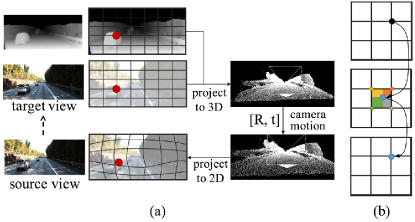
Figure 5: (a) Shows steps of view synthesis using RGB image and its depth map. (b) shows a bilinear interpolation step for adjusting values to pixel space. R and t are rotation and translation parameters. Figure reused from [20]

Most of the monocular, stereo, and MVS depth estimation frameworks use ground truth as a supervision signal. While these frameworks may utilize the additional source view images in the pipeline, they always estimate only one depth map, the reference view depth map. Estimation and use of only one depth map may not provide enough geometrical information for consistent estimation. To address this gap, many methods [31, 20, 49, 54] synthesis additional view (see Fig. 5), either depth map or RGB image (commonly referred to as target view), using camera parameters and reference view information. This additional view, when included in the training framework, provides additional geometric consistency information during the learning process. In this section, we discuss methods that utilize view synthesis in a depth estimation framework.

Bauer et al. [31] use view synthesis in a monocular depth estimation framework. They apply two networks, depth network (DepNet) and synthesis network (SynNet) in a series of operations to enforce geometric constraints with view synthesis. First, the RGB input (source view) is used in DepNet to generate a corresponding depth estimate. The estimated depth map is projected to a target view and using SynNet the holes in the target view are filled. Finally, the synthesized RGB target view is used as input to DepNet to estimate its depth map. This ensures that the DepNet learns to estimate geometrically consistent depth estimates of both the source and the synthesized target view. They use $L_{1}$ loss to enforce consistency.

Yang et al. [20] also synthesize RGB target view to improve geometric consistency in video depth estimation. With estimated pixel matching pairs between source ($I_{s}$) and target views ($I_{t}$), they synthesis a target view $\hat{I}_{s}$ using the source view, camera parameters, and bilinear interpolation [19]. To handle occlusion and movement of objects, an explainability mask ($M_{s}$) is applied during the loss calculation given as

$$\mathcal{L}_{ViewSynthesis}=\sum^{S}_{s=1}|I_{t}-\hat{I}_{s}|\odot M_{s}$$ (11)

where $s$ is the source views.

Typically, MVS methods regularize a cost volume and build using multiple source views, to estimate the reference view depth map. Li et al. [49] argue that by estimating only the reference view depth map from the cost volume, an MVS method underutilizes the information present in the cost volume. They propose a reasonable module to synthesize source depths from the cost volume by projecting the pixels in reference view at different depth hypotheses to the source views. They use robust photometric consistency (Sec. 3.1) to estimate the view synthesis loss.

Dai et al. [54] synthesize source view depth maps using the reference view depth maps in the MVS pipeline for additional geometric consistency. For each pair of reference-source views, they calculate the bidirectional error, i.e. $\mathcal{L}_{r\rightarrow s}$ and $\mathcal{L}_{s\rightarrow r}$ along with $\mathcal{L}_{smooth_{\triangledown}}$ and $\mathcal{L}_{smooth_{\triangledown^{2}}}$ (Sec. 4.2) to estimate $\mathcal{L}_{ViewSynthesis}$. They use a robust formulation of photometric consistency loss (Sec. 3.1) to estimate $\mathcal{L}_{r\rightarrow s}$ and $\mathcal{L}_{s\rightarrow r}$ and add structural similarity (SSIM) error term (Sec. 4.1) in the loss.

$$\mathcal{L}_{ViewSynthesis}^{r\rightarrow s} =(\mathcal{L}_{r\rightarrow s}+\mathcal{L}_{s\rightarrow r})+(\mathcal{L}^{r}_{smooth_{\triangledown}}+\mathcal{L}^{r}_{smooth_{\triangledown^{2}}})$$ (12)

$$\mathcal{L}_{r\rightarrow s} =\mathcal{L}_{photo_{robust}}+\mathcal{L}^{r}_{SSIM}$$ (13)

$$\mathcal{L}_{s\rightarrow r} =\mathcal{L}_{photo_{robust}}+\mathcal{L}^{s}_{SSIM}$$ (14)

where $r,s$ are the reference and the source views. We describe the other loss terms in Sec. 4.

4 Geometry Preserving Constraints

Apart from utilizing cross-view consistency constraints, there are different ways of enforcing structural consistency in a depth estimation pipeline. In this section, we discuss all such approaches that utilize alternative methods of enforcing geometric constraints. We have classified these methods into four broader categories, i.e. structural similarity index measurement (SSIM), edge-aware smoothness constraints, consistency regularization, and planar consistency. We discuss each of these approaches in detail and highlight the research works that utilize these methods in their pipeline.

4.1 Structural Similarity Index Measurement

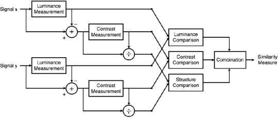
Figure 6: SSIM measurement system as described in [60]. Figure reused from [60]

Objective image quality metrics are roughly classified into three categories based on the availability of distortion-free (original or reference) images. The metric is called full-reference when the complete reference image is known, it is called no-reference when the reference image is not available and it is called reduced-reference when the reference image is partially available. Eskicioglu and Fisher [61] discuss several such image quality metrics and their performance.

Structural similarity index measurement (SSIM) is a full-reference image quality assessment technique [60]. Its assessment is based on the degradation of structural information between the reference and the noisy image. Specifically, it compares local patterns of pixel intensities that have been normalized for luminance and contrast. Luminance of a surface is the product of its illumination and reflectance, but the structure of the object is independent of illumination. SSIM separates the influence of illumination to analyze the structural information in an image.

Wang et al. [60] define structural information as the attributes that represent the structural information of objects in an image, independent of average luminance and contrast. As shown in Fig. 6, given two aligned non-negative signals (images), X and Y, one of which is assumed to be the reference quality, we can have a quantitative measurement of the second signal with SSIM. Three separate tasks are considered for structural similarity measurement: luminance, contrast, and structure [60].

$$\mu_{x}=\frac{1}{N}\sum^{N}_{i=1}x_{i};\mu_{y}=\frac{1}{N}\sum^{N}_{i=1}y_{i}$$ (15)

$$\sigma_{x}=(\frac{1}{N-1}\sum^{N}_{i=1}(x_{i}-\mu_{x})^{2})^{\frac{1}{2}};\sigma_{y}=(\frac{1}{N-1}\sum^{N}_{i=1}(y_{i}-\mu_{y})^{2})^{\frac{1}{2}}$$ (16)

$$\sigma_{xy}=\frac{1}{N-1}\sum^{N}_{i=1}(x_{i}-\mu_{x})(y_{i}-\mu_{y})$$ (17)

The SSIM formula is given in Eq. 18, which is a scaled product of the three components discussed above. The luminance comparison function $l(X,Y)$ is a function of mean intensities $\mu_{x}$ and $\mu_{y}$ as shown in Eq. 19. The contrast comparison $c(X,Y)$ is a function of $\sigma_{x}$ and $\sigma_{y}$ as shown in Eq. 20 and the structure comparison measure $s(X,Y)$ is a function of correlation coefficient $\sigma_{xy}$, $\sigma_{x}$ and $\sigma_{y}$ as shown in Eq. 21. $L$ is the dynamic range of the pixel values (255 for grayscale image). The mean, standard deviation, and correlation coefficient of the signals are calculated using Eqs. 15, 16, and 17. Where $N$ is the total number of pixels in an image.

$$SSIM(X,Y) =[l(X,Y)]^{\alpha}.[c(X,Y)]^{\beta}.[s(X,Y)]^{\gamma};\alpha>0,\beta>0,\gamma>0$$ (18)

$$l(X,Y) =\frac{2\mu_{x}\mu_{y}+c_{1}}{\mu_{x}^{2}+\mu_{y}^{2}+c_{1}};c_{1}=(K_{1}L)^{2},K_{1}\ll 1$$ (19)

$$c(X,Y) =\frac{2\sigma_{x}\sigma_{y}+c_{2}}{\sigma^{2}_{x}+\sigma^{2}_{y}+c_{2}};c_{2}=(K_{2}L)^{2},K_{2}\ll 1$$ (20)

$$s(X,Y) =\frac{\sigma_{xy}+c_{3}}{\sigma_{x}\sigma_{y}+c_{3}},c_{3}=\frac{c_{2}}{2}$$ (21)

SSIM index should be applied locally rather than globally for the following reasons. First, image statistical features are highly spatially non-stationary. Second, image distortions may be space-variant, and third, local quality measurement delivers more information about the quality degradation by providing a spatially varying quality map of the image.

Wang et al. [60] defined $SSIM$ index for two signals in the same domain, i.e. it can estimate the structural similarity between two RGB or grayscale images or between two depth maps or two patches. In an end-to-end framework, where we minimized the loss, we want to maximize $SSIM$ for better result. Since $SSIM$ is upper bound to $1$, we can instead minimize $1-SSIM$. This formulation takes a general form of

$$\mathcal{L}_{SSIM}=\frac{1}{N}\sum^{N}_{i=1}\frac{1-SSIM(X,Y)}{K}\odot M$$ (22)

in an end-to-end depth estimation framework. Where $N$ is the number of source views, $X$ and $Y$ are the two signals to be compared, preferably in the same domain. $M$ is the mask to handle occlusion and $K$ is a constant.

Zhao et al. [62] use this formulation with no mask and $K=1$ for image restoration problems. It calculates the means and standard deviations (Eqs. 15, 16 and 17) using Gaussian filter with standard deviation $\sigma_{G}$. The choice of $\sigma_{G}$ impacts the quality of the processed results. With smaller values of $\sigma_{G}$ the network loses the ability to preserve local structures, introducing artifacts in the image, and for larger $\sigma_{G}$, the network preserves noises around the edges. Instead of finetuning the value of $\sigma_{G}$, Zhao et al. [62] propose a multi-scale formulation of SSIM (MS-SSIM), where all results from the variations of $\sigma_{G}$ are multiplied together.

Inherently, both MS-SSIM and SSIM are not particularly sensitive to the change of brightness or shift of colors. However, they preserve the contrast in high-frequency regions. $L_{1}$ loss, on the other hand, preserves colors and luminance - an error weighted equally regardless of the local structure - but does not produce the same impact for contrast. For best impact, Zhao et al. [62] combines both these terms, $\mathcal{L}^{mix}_{SSIM}$, as follows

$$\mathcal{L}^{mix}_{SSIM}=\alpha.\mathcal{L}_{SSIM}+(1-\alpha).\mathcal{L}^{l_{i}}$$ (23)

where, $\alpha$ is a tunable hyper-parameter and $l_{i}$ is $L_{1}$ or $L_{2}$ norm.

Mallick et al. [44] use simplest form of $\mathcal{L}_{SSIM}$ (Eq. 22) in a self-supervised MVS framework with no mask $M$, $X=I_{ref}$, $Y=\hat{I}_{src}$ and $K=1$. Huang et al. [22] use $\mathcal{L}_{SSIM}$ (Eq. 22) with $X=I_{ref}$, $Y=\hat{I}_{src}$ and $K=2$ in unsupervised MVS framework. Mahjourian et al. [25] also use it in unsupervised MVS framework with $K=1$ (Eq. 22), $c_{1}={0.01}^{2}$ and $c_{2}={0.03}^{2}$ (Eqs. 19 and 20). Khot et al. [48] use the same formulation as [25] in an unsupervised MVS framework. Li et al. [49] use bidirectional calculation, forward ($\mathcal{L}^{forward}_{SSIM}$) with $X=I_{ref}$, $Y=\hat{I}_{src}$ (Source view projected to reference view) and backward ($\mathcal{L}^{backward}_{SSIM}$) with $X=\hat{I}_{ref}$, $Y=I_{src}$ (reference view projected to source view), with no mask $M$ and $K=1$, Eq. 22. The final $\mathcal{L}_{SSIM}=\mathcal{L}^{forward}_{SSIM}+\mathcal{L}^{backward}_{SSIM}$

As explained earlier, the $\mathcal{L}_{SSIM}$ is usually combined with a uniformly weighted loss function like $L_{1}$ and $L_{2}$, to choose the best of both the individual loss terms. The combined formulation is shown in Eq. 23. Dai et al. [54] and Yu et al. [52] use Eq. 23 formulation with $\alpha=0.85$ in MVS framework. This formulation finds widespread use in monocular depth estimation problems. Monocular methods like, [63, 64] uses Eq. 23 with $\alpha=0.85$ with target and novel view synthesized depth maps as $X$ and $Y$. Godard et al. [26] use $\mathcal{L}^{mix}_{SSIM}$ (Eq. 23) between input RGB image and reconstructed new view RGB image with $\alpha=0.85$ to enforce structural similarity. Zhao et al. [65] with symmetric domain adaptation, real-to-synthetic and synthetic-to-real, apply Eq. 23 both ways to enforce structural similarity during the transition from one domain to the other domain.

Chen et al. [23] use $\mathcal{L}^{mix}_{SSIM}$, Eq. 23, with slight modification to make it adaptive loss in optical flow estimation problem. For scene structures that can not be explained by the global rigid motion, it adapts to a more flexible optical flow estimation by updating the channel parameters only for the configurations that closely explain the displacement. It is represented as the minimum error between the optical flow and the rigid motion displacements, it is formulated as

$$L^{adaptive}_{SSIM}=min\{\mathcal{L}^{mix}_{SSIM_{flow}},\mathcal{L}^{mix}_{SSIM_{rigid}}\}$$ (24)

where it uses $\alpha=0.85$ in Eq. 23. We only discuss the $\mathcal{L}^{mix}_{SSIM}$ formulation here and refer to [23] for other optical flow related details.

4.2 Edge-Aware Smoothness Constraint

The smoothness constraint finds its origin in the optical flow estimation problem. It was first applied by Uras et al. [66] to estimate consistent optical flow from two images. Brox et al. [67] further explained the concept under three assumptions for the optical flow framework, i.e. the gray value constancy assumption, the gradient constancy assumption, and the smoothness assumption.

$$I(x,y,t) =I(x+u,y+v,t+1)$$ (25)

$$\triangledown I(x,y,t) =\triangledown I(x+u,y+v,t+1)$$ (26)

$$E_{smooth}(u,v) =\int\psi(|\triangledown u|^{2}+|\triangledown v|^{2})dx$$ (27)

Since the beginning of the optical flow estimation problem, it has been assumed that the gray value of a pixel does not change on displacement under a given lighting condition, Eq. 25 [67]. But brightness changes in a natural scene all the time. Therefore, it is considered useful to allow small variations in gray values but finds a different criterion that remains relatively invariant under gray value changes, i.e. the gradient constancy was assumed under displacement, Eq. 26. This brought about the third assumption, the smoothness of the flow field. While discontinuities are assumed to be present at the boundaries of the object in the scene, a piecewise smoothness can be assumed in the flow field [67]. To achieve this smoothness in flow estimation a penalty on the flow field was applied as shown in Eq. 27.

In the optical flow framework, objects are assumed to be moving with a fixed camera, in an MVS framework, the objects are assumed to be fixed and the camera moves concerning a fixed point. The relative motion of an object can be viewed as a moving camera to pose it as an MVS problem, see Fig. 4. With this assumption, the smoothness constraint can be applied to the depth estimation problem. Initially, only the first-order smoothness constraints were used in the depth estimation framework [27, 19, 26, 64, 25, 52]. After Yang et al. [20] used second-order smoothness constraint for regularization was combined with the first-order smoothness constraint in subsequent works [54, 22, 50, 68].

$$\mathcal{L}_{smooth_{\triangledown}} =\sum||\partial_{x}\hat{D}||.e^{-||\partial_{x}I||}+||\partial_{y}\hat{D}||.e^{-||\partial_{y}I||}$$ (28)

$$\mathcal{L}_{smooth_{\triangledown^{2}}} =\sum||\partial^{2}_{x}\hat{D}||.e^{-||\partial^{2}_{x}I||}+||\partial^{2}_{y}\hat{D}||.e^{-||\partial^{2}_{y}I||}$$ (29)

$$\mathcal{L}_{smooth} =\alpha.\mathcal{L}_{smooth_{\triangledown}}+\beta.\mathcal{L}_{smooth_{\triangledown^{2}}}$$ (30)

In the depth estimation framework, smoothness constraint is applied between the gradient of input images $(I)$ and the estimated depth maps $(\hat{D})$. Eqs. 28 and 29 represents the first $(\mathcal{L}_{smooth_{\triangledown}})$ and second $(\mathcal{L}_{smooth_{\triangledown^{2}}})$ order smoothness constraints. Eq. 30 shows the combined formulation with $\alpha>0$ and $\beta>0$ as a scaling factor.

Garg et al. [19] use the first order formulation with $L_{2}$ norm as a regularization term to achieve smoothness in estimation. Mahjourian et al. [25] use the first order formulation for monocular video depth estimation problem. First-order smoothness constraint is actively used in self-supervised/unsupervised MVS frameworks [49, 52, 47, 48, 44]. Zhao et al. [65] with its symmetric domain adaptation for monocular depth estimation uses first-order constraint in both domains. Other monocular depth estimation methods [26, 64, 69, 63] also apply the first-order smoothness constraint as defined in Eq. 28.

Yang et al. [20] only uses second order formulation, Eq. 29 as a regularization term in monocular video-depth estimation framework. Learning from it, more recent MVS frameworks combine both the first-order and the second-order formulation [22, 54, 50] as shown in Eq. 30. Inspired from [26] and [69], Yang et al. [68] apply the combined edge-aware smoothness constraint, Eq. 30, in monocular endoscopy problem. All these methods use $\alpha=\beta=1$ in Eq. 30.

4.3 Consistency Regularization

Deep learning-based frameworks inherently suffer from over-parameterization problems. One of the most efficient methods to counter it is to regularize the loss function. Photometric consistency, Sec. 3.1, which enforces geometrical consistency at the pixel level is highly susceptible to change in lighting conditions. Many MVS methods employ different consistency regularization techniques to effectively handle this problem [20, 19, 51].

As discussed in Sec 4.2, first-order and second-order gradients are often used for this task [20, 19]. Garg et al. [19] argue that the photometric loss is non-informative in homogeneous regions of a scene, which leads to multiple warps generating similar disparity outcomes. It uses $L_{2}$ regularization (Eq. 31) on the disparity discontinuities as a prior. It also recommends the use of other robust penalty functions used in [67, 70] as an alternative regularization term. Yang et al. [20] use a spatial smoothness penalty with $L_{1}$ norm of second-order gradient of depth, Eq. 32. It encourages depth values to align in the planar surface when no image gradient appears.

Xu et al. [51] apply consistency regularization in the semi-supervised MVS method. The proposed regularization minimizes the Kullback-Leibler (KL) divergence between the predicted distributions of augmented $(\hat{PV})$ and non-augmented $(PV)$ samples. With the $K$ depth hypothesis, the probability volume $PV$, of size $H\times W\times K$, is separated into $K$ categories of $HW$ logits. Eq. 33 shows the formulation of the regularizer, where $p_{i}$ represents a pixel coordinate.

$$\mathcal{L}_{\triangledown} =||\triangledown\hat{D}||^{2}$$ (31)

$$\mathcal{L}_{\triangledown^{2}} =\sum_{d\in x,y}|\triangledown^{2}_{d}\hat{D}|.e^{-\alpha|\triangledown I|};\alpha>0$$ (32)

$$\mathcal{L}_{KL} =\frac{1}{HW}\sum^{HW}_{i=1}KL(PV_{p_{i}},\hat{PV}_{p_{i}})$$ (33)

4.4 Structural Consistency in 3D Space

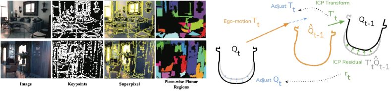
Figure 7: Left: Example of an input image, their corresponding key points, superpixels and piece-wise planar regions obtained from large superpixels (Fig. reused from [52]). Right: Point cloud matching process and approximate gradients for the top view of a car (Fig. reused from [25]).

Structural consistency is not limited to the 2D image plane, it can easily be extended to camera 3D space or 3D point clouds. In this section, we discuss two such methods [52, 25] that uses structural consistency in 3D space alongside other geometric constraints in an end-to-end framework.

4.4.1 Planar Consistency

Planar consistency [52] is based on the assumption that most of the homogeneous-color regions in an indoor scene are planar regions and a continuous depth can be assumed for such regions. Extraction of such piece-wise planar regions is a three-step process. Given an input image $I$, first, the key points are extracted. The key points in the input image are then used to extract superpixels. Finally, a segmentation algorithm is used to apply a greedy approach to segment areas with low gradients to produce more planar regions. There are many ways to extract key points and superpixels, [52] uses Direct Sparse Odometry [53] to extract key points and Felzenszwalb superpixel segmentation [71] for superpixels and planar regions segmentation.

Left side images in Fig. 7 show the steps of obtaining planar regions in two indoor scenes. For an image $I$, after extracting the superpixels, a threshold is applied to only keep regions with larger than $1000$ pixels. It is assumed that most planar regions occupy large pixel areas. With the extracted super pixels $SPP_{m}$ and its corresponding depth $D(p_{n})$, we first back project all points $p_{n}$ into 3D space ($p^{3D}_{n}$), Eq 34. Using the plane parameter $A_{m}$ of $SPP_{m}$, the plane is defined in 3D space, Eq. 35. $A_{m}$ is calculated using two matrices, $Y_{m}=[1,...,1]^{T}$ and $P_{n}=[p^{3D}_{1},...,p^{3D}_{n}]$ as shown in Eq. 36, where $E$ is an identity matrix and $\epsilon$ is a for numerical stability. With planar parameters, a fitted planar depth for each pixel in all superpixels can be retrieved to estimate the planar loss $\mathcal{L}_{planar}$ as shown in Eq. 38

$$p^{3D}_{n} =D(p_{n})K^{-1}p_{n},p_{n}\subseteq SPP_{m}$$ (34)

$$A^{T}_{m}p^{3D}_{n} =1$$ (35)

$$P_{n}A_{m} =Y_{m};A_{m}=(P^{T}_{n}P_{n}+\epsilon E)^{-1}P^{T}_{n}Y_{m}$$ (36)

$$D^{\prime}(p_{n}) =(A^{T}_{m}K^{-1}p_{n})^{-1}$$ (37)

$$\mathcal{L}_{planar} =\sum^{M}_{m=1}\sum^{N}_{n=1}|D(p_{n})-D^{\prime}(p_{n})|$$ (38)

4.4.2 Point Cloud Alignment

Mahjourian et al. [25] use another approach to align the 3D point clouds of two consecutive frame ($Q_{t-1},Q_{t}$) in video depth estimation pipeline. It directly compares the estimated point cloud associated with respective frames ($\hat{Q}_{t-1}$ and $\hat{Q}_{t}$), i.e. compare $\hat{Q}_{t-1}$ to $Q_{t-1}$ or $\hat{Q}_{t}$ to $Q_{t}$ using well know rigid registration methods, Iterative Closest Point (ICP) [72, 73, 74], that computes a transformation to minimize the point-to-point distance between two point clouds. It alternates between computing correspondences between 3D points and best-fit transformation between the two point clouds. For each iteration, it recomputes the correspondence with the previous iteration’s transformation applied.

ICP is not differentiable, but its gradients can be approximated using the products it computes as part of the algorithm, allowing back-propagation. It takes two point clouds $A$ and $B$ as input and produces two outputs. First is the best-fit transformation $T^{\prime}$ which minimizes the distance between the transformed points in $A$ and $B$, and second is the resudual $r^{ij}$, Eq. 39, which reflects the residual distances between corresponding points after ICP’s minimization. The loss, $\mathcal{L}_{3DAlignment}$, is given as in Eq. 40.

$$r^{ij} =A^{ij}-T^{\prime-1}.B^{c(ij)}$$ (39)

$$\mathcal{L}_{3DAlignment} =||T^{\prime}-I||_{1}+||r||_{1};I=1$$ (40)

For each frame $t$ of the video, if the alignment of the estimate is not perfect, the ICP algorithm produces a transformation $T^{\prime}_{t}$ and $r_{t}$, which can be used to adjust the estimates towards initial alignment [25]. Right side of Fig. 7 shows the steps of alignment loss.

5 Normal-Depth Orthogonal Constraint

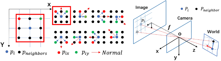
Figure 8: Left: estimation of normal from depth. Right: estimation of depth from normal. Figure reused from [22]

Surface normal is an important ’local’ feature of 3D point-cloud of a scene, which can provide promising 3D geometric cues to estimate geometrically consistent depth maps. In the 3D world coordinate system, the vector connecting two pixels in the same plane should be orthogonal to their direction of normal. Enforcing normal-depth orthogonal constraint tends to improve depth estimates in 3D space [75, 27, 20].

Depth to normal:

Given depth $D_{i}$, to estimate the normal of each central pixel $p_{i}$, Fig. 8 (left), we need to consider the neighboring pixels, $p_{neighbors}$. The Fig. 8 (left) shows $8$ neighbor convention to compute the normal of the central pixel. Two neighbors , $p_{ix}$ and $p_{iy}$ are selected from $p_{neighbors}$ for each central pixel $p_{i}$ with depth value as $D_{i}$ and camera intrinsics $K$ to estimate normal $\tilde{N_{i}}$. First, we project the depth in 3D space and then, use cross product between vector $\overrightarrow{P_{i}P_{ix}}$ and $\overrightarrow{P_{i}P_{iy}}$ to estimate the normal, Eq. 42. With $8$ such estimates of normal $\tilde{N_{i}}$ for each central pixel, we estimate the final normal $N_{i}$ as the mean value of all the estimates using Eq. 43.

$$P_{i} =K^{-1}D_{i}p_{i}$$ (41)

$$\tilde{N_{i}} =\overrightarrow{P_{i}P_{ix}}\times\overrightarrow{P_{i}P_{iy}}$$ (42)

$$N_{i} =\frac{1}{8}\sum^{8}_{i=1}(\tilde{N_{i}})$$ (43)

Normal to depth:

Many methods [22, 20, 76] use normal to depth estimation to refine the depth values $D_{i}$ using the orthogonal relationship. For each pixel $p_{i}(x_{i},y_{i})$, the depth of each neighbor $p_{neighbor}$ should be refined. The corresponding 3D points are, $P_{i}$ and $P_{neighbor}$ and central pixel $P_{i}$’s normal $\overrightarrow{N_{i}}(n_{x},n_{y},n_{z})$. The depth of $P_{i}$ is $D_{i}$ and $P_{neighbor}$ is $D_{neighbor}$. Using the orthogonal relations $\overrightarrow{N_{i}}\perp\overrightarrow{P_{i}P_{neighbor}}$, we can write the Eq. 44. With depth estimates coming from eight neighbors, we need a method for weighting these values to incorporate discontinuity of normal in some edges or irregular surfaces. Generally, the weight $w_{i}$ is inferred from the reference image $I_{i}$, making depth more conforming to geometric consistency. The value of $w_{i}$ depends on the gradient between $p_{i}$ and $p_{neighbor}$, Eq. 45. The bigger values of gradient represent the less reliability of the refined depth. Given the eight neighbors, the final refined depth $\tilde{D}_{neighbor}$ is a weighted sum of eight different directions as shown in Eq. 46 [22]. This is the outcome of the regularization in 3D space, improving the accuracy and continuity of the estimated depth maps.

$$[K^{-1}D_{i}p_{i}-K^{-1}D_{neighbor}P_{neighbor}]\begin{bmatrix}n_{x}\\ n_{y}\\ n_{z}\\ \end{bmatrix} =0$$ (44)

$$w_{i} =e^{-\alpha|\triangledown I_{i}|}$$ (45)

$$\tilde{D}_{neighbor} =\sum^{8}_{i=1}\frac{w_{i}}{\sum^{8}_{i=1}w_{i}}D_{neighbor}$$ (46)

Yang et al [20] use a similar formulation as shown in Eqs. 44, 45, and 46 to enforce geometric consistency in unsupervised video depth estimation problems. Wang et al. [75] use the orthogonal compatibility principle to bring consistency in the normal directions of two pixels falling on the same plane. Eigen and Fergus [27] use a single multiscale CNN to estimate depth, surface normal, and semantic labeling. For surface normal estimation at each pixel, they predict the $x,y$ and $z$ components for each pixel [77] and employ elementwise loss comparison with dot product as shown in Eq. 47, where $N$ is the valid pixels, $n$ and $\hat{n}$ are ground truth and the predicted normal at each pixel.

$$\mathcal{L}_{normal}=-\frac{1}{N}\sum_{i}\hat{n}_{i}.n_{i}$$ (47)

Qi et al. [78] also employ depth-to-normal and normal-to-depth networks to regularize the depth estimate in 3D space following [79], but they do not use 8-neighbor-based calculation. Instead, they use a distance-based selection of neighboring pixels are given as

$$N_{i}=\{(x_{j},y_{j},z_{j})||u_{i}-u_{j}|<\beta,|v_{i}-v_{j}|<\beta,|z_{i}-z_{j}|<\gamma z_{i}\}$$ (48)

where, $u_{i},v_{i}$ are the 2D coordinates, $(x_{i},y_{i},z_{i})$ are the 3D coordinates, $\beta$ and $\gamma$ are hyper-parameters controlling the size of the neighborhood along $x-y$ and depth axes respectively. They use $L_{2}$ norm between the ground truth normal and the estimated normal as the loss $\mathcal{L}_{normal}$ in end-to-end deep learning framework.

Hu et al. [69] use ground truth and estimated depth map gradients to measure the angle between their surface normals, Eqs. 49 and 50. The loss, $\mathcal{L}_{normal}$ is estimated as per Eq. 51, where $\langle.,.\rangle$ denotes the inner product of vectors. This loss is sensitive to small depth structures [69]. Yang et al. [68] use the same method of estimating normal for monocular depth estimation problems in Endoscopy applications.

$$n^{\hat{d}}_{i} =[-\triangledown_{x}\hat{d}_{i},-\triangledown_{y}\hat{d}_{i},1]^{T}$$ (49)

$$n^{d}_{i} =[-\triangledown_{x}d_{i},-\triangledown_{y}d_{i},1]^{T}$$ (50)

$$\mathcal{L}_{normal} =\frac{1}{N}\sum^{N}_{i=1}\left(1-\frac{\langle n^{\hat{d}}_{i},n^{d}_{i}\rangle}{\sqrt{\langle n^{\hat{d}}_{i},n^{\hat{d}}_{i}\rangle}\sqrt{\langle n^{d}_{i},n^{d}_{i}\rangle}}\right)$$ (51)

There are several advantages of estimating normal in a depth estimation framework, like, it provides an explicit understanding of normal during the learning process, it provides higher-order interaction between the estimated depth and ground truths and it also provides flexibility to integrate additional operations, e.g. Manhattan assumption, over normal [20]. It also has certain disadvantages, like, as it is prone to noise in the ground truth depth maps or the estimated depth maps and it only considers local information for its estimation which may not align with the global structure.

$$\mathcal{L}_{Normal_{robust}}=\frac{1}{N}\left(\sum^{N}_{i=1}||\hat{n}-n_{i}||_{1}\right)$$ (52)

To enforce robust higher-order geometric supervision in 3D space, Yin et al. [76] propose virtual normal (VN) estimation. VN can establish 3D geometric connections between regions in a much larger range. To estimate VN, $N$ group points from the depth map, with three points in each group, are sampled. The selected point has to be non-colinear. The three points establish a plane and the corresponding normal is estimated. Similarly, ground truth normal $(n_{i})$ are estimated and compared with the normal corresponding to the estimated depth maps $(\hat{n}_{i})$ as shown in Eq. 52. Naderi et al. [30] use a similar formulation in a monocular depth estimation problem to enforce higher-order robust geometric constraints for depth estimation.

Normal-depth joint learning approach:

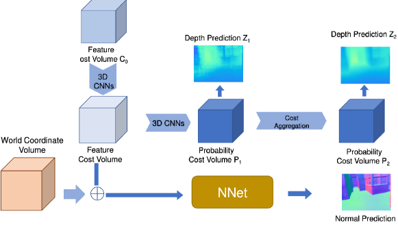
Figure 9: Normal-depth joint learning approached. Depth and normal are estimated using the same feature cost volume [80]. The above diagram is a slight modification from Kusupati et al [80] to only show the joint estimation setup.

Kusupati et al. [80] develop a normal-assisted depth estimation algorithm that couples the learning of multi-view normal estimation and multi-view depth estimation process. It utilizes feature cost volume to estimate the depth map and the normal. A cost volume provides better structural representation to facilitate better learning on the image features for estimating the underlying surface normal. Specifically, Kusupati et el. [80] estimates two depth maps $Z_{1}$ and $Z_{2}$ using 3D-CNNs, see Fig. 9, and utilizes a 7-layered CNN (NNet, Fig. 9) to estimate normal. The world coordinate volume is concatenated with the initial feature volume to provide a feature slice to NNet as input. NNet predicts normal for each feature slice, which is later averaged to get the final normal map.

6 Attention Meets Geometry

A transformer with a self-attention mechanism is introduced by Dosovitski et al. [12] in vision domain. It can learn long-range global-contextual representation by dynamically shifting its attention within the image. The inputs to the attention module are usually named query (Q), key (K), and value (V). Q retrieves information from V based on the attention weights, Eq. 53, where $\mathcal{A}(.)$ is a function that produces similarity score as attention weight between feature embeddings for aggregation.

The performance of stereo or MVS depth estimation methods depends on finding dense correspondence between reference images and source images. Recently, Sun et al. [81] showed that features extracted using a transformer model with self- and cross-attention can produce significantly improved correspondences as compared to the features extracted using convolutional neural networks. These attention mechanisms are designed to pay attention to the contextual information and not to geometry-based information. Recently, a few methods have modified these attention mechanisms to consider geometric information while calculating the attention weight [82, 30, 83, 84]. In this section, we discuss such methods and their approach to include geometric information in attention.

$$Attention(Q,K,V) =\mathcal{A}(Q,K)V$$ (53)

$$p_{i}=K^{-1}(d_{i}.C_{i});p_{j} =K^{-1}(d_{j}.C_{j})$$ (54)

$$\mathcal{A}^{spatial}_{i,j} =exp\left(-\frac{||P_{i}-P_{j}||_{2}}{\sigma}\right)$$ (55)

$$\mathcal{A}^{temporal}_{i,j} =Softmax_{j}(F^{q^{T}}_{i}F^{k}_{j})$$ (56)

Ruhkamp et al. [82] use geometry to guide spatial-temporal attention to guide self-supervised monocular depth estimation method from videos. They propose a spatial-attention layer with 3D spatial awareness by exploiting a coarse predicted initial depth estimate. With known intrinsic camera parameter K and pair of coordinates ($C_{i},C_{j}$) along with their depth estimates $(d_{i},d_{j})$, they back-project the depth values into 3D space using Eq. 54. The 3D space-aware spatial attention is then calculated as per Eq. 55, where $P_{i},P_{j}$ are treated as K and Q, respectively. They use Eq. 56 to estimate the temporal attention for aggregation. The unique formulation of the spatial-temporal attention model can explicitly correlate geometrically meaningful and spatially coherent features for dense correspondence [82].

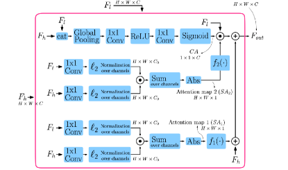
Figure 10: Adaptive Geometric Attention. Figure reused from [30]

Naderi et al. [30] propose adaptive geometric attention (AGA) for monocular depth estimation problems with encoder-decoder architecture. They apply the AGA module in the decoding step utilizing both low-level $(F_{L})$ and high-level $(F_{h})$ features. Fig. 10 shows the process of calculating AGA. The first row of operation in Fig. 10 shows the steps to calculate channel-attention $(\mathcal{CA})$, which produces $1\times 1\times C$ shape attention map and is multiplied with the $F_{l}$. Rest, two rows of calculation shows two spatial attention $(\mathcal{SA})$ calculation which is equivalent to Eq. 57. The final aggregated feature output $(F_{o}ut)$ is estimated using Eq. 60, where $\mathcal{SA}_{1}$ is added and $\mathcal{SA}_{2}$ is multiplied with $F_{L}$. $f_{1}(.)$ and $f_{2}(.)$ are introduced to enhance the sensitivity to any non-zero correlation between $F_{l}$ and $F_{h}$, Eq. 58 is the with no-enhanced sensitivity, whereas Eq. 59 shows the formulation of sensitivity enhanced attention map.

$$\mathcal{SA}_{i} =|Cosine_{similarity}(E_{l,i},E_{h,i})|,i=1,2$$ (57)

$$f(\mathcal{SA}) =\mathcal{SA}$$ (58)

$$f(\mathcal{SA}) =\mathcal{SA}.\,exp(\mathcal{SA})$$ (59)

$$F_{out} =[f_{1}(\mathcal{SA}_{1})+f_{2}(\mathcal{SA}_{2})\times\mathcal{CA}]\times F_{l}+F_{h}$$ (60)

Zhu et al. [83] use two types of transformer modules to extract geometry-aware features in an MVS pipeline, a global-context transformer module and a 3D geometry transformer module. The global-context transformer module extracts 3D-consistent reference features $(T_{r})$ which is then used as input to the 3D-geometry transformer module to facilitate cross-view attention. $(T_{r})$ is used to generate K and V to enhance interaction between reference and source view features for obtaining dense correspondence.

Guo et al. [84] use a geometrically aware attention mechanism for image captioning tasks. Unlike other methods discussed above, they do not modify the attention mechanism in itself but add a bias term which makes the feature extraction biased towards specific content. Their attention module is similar to [12] apart from the added bias term in score $E$ calculation, Eq. 61, where $G_{ij}$ is the relative geometry feature between two objects $i$ and $j$. There are two terms in score $E$, the left one is content-based weights and the right one is geometric bias. They propose three different ways of applying geometric bias. content-independent bias (Eq. 62) assumes static geometric bias, i.e. same geometric bias is applied to all the K-Q pairs. The query-dependent bias provides geometric information based on the type of query (63) and key-dependent bias provides geometric information based on the clues present in keys (Eq. 64).

$$E =QK^{T}+\phi(Q^{\prime},K^{\prime},G)$$ (61)

$$\phi^{independent}_{ij} =ReLU(w^{T}_{g}G_{ij})$$ (62)

$$\phi^{query}_{ij} =Q^{{}^{\prime}T}_{g}G_{ij}$$ (63)

$$\phi^{key}_{ij} =K^{{}^{\prime}T}_{g}G_{ij}$$ (64)

7 Learning Geometric Representations

Apart from utilizing direct methods of enforcing geometric constraints or providing geometric guidance or exploiting orthogonal relations between depth and normal, there are some indirect ways of learning geometrically and structurally consistent representations. For example, features with high-level of semantic information is more likely to retain structural consistency of objects compared to features with low-level of semantic information, pseudo-label generation purely on the basis of geometric consistency can be utilized for self-supervision, more robust feature representation can be learned using suitable data-augmentation techniques, attaching semantic segmentation information of objects or using co-segmentation can also provide suitable clues for the structural consistency of objects, contrastive learning with positive and negative pairs can guide a model to learn better representation which are geometrically sharp and consistent. We discuss all such methods in this section.

7.1 High-Level Feature Alignment Constraints

In deep learning-based frameworks for depth estimation, the quality of the extracted features directly impacts the quality of depth estimates. The poor quality of extracted features can greatly impact the local as well as global structural pattern. One way to handle this problem is by guiding the extracted features with better representation from an auxiliary pre-trained network. While the integrated feature extraction network in the depth estimation pipeline can learn useful features, it still lags in learning higher-level representations compared to a network explicitly designed to learn deep high-level representations like, VGG [85], Inception [86], ResNet [87] etc. To enforce the feature alignment constraint, Johnson et al. [88] propose two loss functions, feature reconstruction loss and style reconstruction loss.

Feature reconstruction loss, Eq. 66, encourages the model to generate source features similar to the target features at various stages of the network [88]. Minimizing feature reconstruction loss for early layers improves local visual as well as structural patterns, while minimizing it for higher layers improves overall structural patterns [88]. Feature reconstruction loss fails to preserve color and texture, which is handled by style reconstruction loss [88].

$$\mathcal{L}_{feature} =||F_{target}-F_{source}||_{L_{i}}$$ (66)

$$\mathcal{L}_{feature} =\frac{1}{N}\sum\left(F_{ref}-\hat{F}_{src}\right).M_{ref}$$ (67)

Eq. 66 shows the generalized formulation of feature reconstruction loss, where $F_{target}$ is the target feature, $F_{source}$ is the source feature and $L_{i}$ denotes $L_{1}$ or $L_{2}$ norm. A similar formulation is adopted by Huang et al. [22], dubbed as feature-wise loss, in an unsupervised MVS framework. Using a pre-trained VGG-16 network, high-level semantically rich feature is extracted at layers 8, 15, and 22 for both the reference $(F_{ref})$ and the source $(F_{src})$ images. The features from the source images are warped to the reference view $(\hat{F}_{src})$ using camera parameters and used in feature reconstruction loss as shown in Eq. 67. $M$ is the reference view mask to handle occlusion and $N$ is the number of source view images. Dong et al. [50] use similar formulation and extract feature from $8^{th}$ and $15^{th}$ layers

Applying feature alignment loss helps the model extract high-level semantically rich features for depth estimation, it can also be used to generate geometrically consistent and style-conforming new RGB image, which is then used as input to the depth estimation network. Zhao et al. [65] and Xu et al. [51] use such an approach to fill generate synthetic input images that are geometrically consistent across views and close to the original data distribution.

Zhao et al. [65] generate synthetic RGB images, they apply feature reconstruction and style reconstruction loss at final image resolution. They learn bidirectional translators from source to target, $G_{s2t}$ and target to source $G_{t2s}$ to bridge the gap between the source domain (synthetic) $X_{s}$ and the target domain (real) $X_{t}$. Specifically, image $x_{s}$ is sequentially fed to $G_{s2t}$ and $G_{t2s}$ generating a reconstruction of $x_{s}$ and vice-versa for $x_{t}$. These are then compared to the original input as follows

$$\mathcal{L}_{Feature_{cycle}}=||G_{t2s}(G_{s2t}(x_{s}))-x_{s}||_{1}+||G_{s2t}(G_{t2s}(x_{t}))-x_{t}||_{1}$$ (68)

While Zhao et al. [65] apply $\mathcal{L}_{feature_{cycle}}$ at RGB image level, Xu et al. [51] use feature and style reconstruction loss in semi-supervised MVS framework. They use a geometry-preserving module to generate geometry and style-conforming RGB images using a labeled real image. They employ a geometry geometry-preserving module to generate unlabeled RGB images which are later used as input to estimate depth maps. The geometry-preserving module includes a spatial propagation network (SPN) with two branches - propagation network and guidance network. The labeled image $(I_{l})$ is used as input to the guidance network to generate an alternate view RGB image $(I_{g})$. This RGB image is used as input to the depth estimation pipeline to generate a corresponding depth map $D_{g}$. $D_{g}$ is then warped to the original view ($\hat{D}_{g}$) to compare with the ground truth depth map $D_{l}$. Eq. 69 shows the formulation of the loss function used in [51]. With this setup, they use labeled images to generate geometrically conforming alternate view unlabeled images and use them in the depth estimation pipeline without having to create new labeled data.

$$\mathcal{L}_{feature_{style}}=||D_{l}-\hat{D}_{g}||^{2}_{2}$$ (69)

7.2 Pseudo-Label Generation with Cross-View Consistency

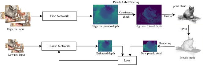
Figure 11: Pseudo-label generation method of [21]. SPSR is Screened Poisson Surface Reconstruction method [89]. Figure inspired from [21]

In self-supervised MVS frameworks, one of the effective methods of applying geometric constraints is by generating pseudo-labels. Generating pseudo-labels requires application of cross-view consistency constraints, which encourages the MVS framework to be geometrically consistent during training and evaluation [21, 47]. Since the model learns with self-supervision, it also helps with the challenging task of collecting multi-view ground truth data. In this section, we discuss three methods of generating pseudo-labels for self-supervision, labels from high-resolution training images [21], sparse pseudo-label generation [47] and semi-dense pseudo-label generation [47].

Yang et al. [21] apply pseudo-label learning in four steps. First, they estimate the depth map based on photometric consistency, Sec. 3.1, using a coarse network (low-resolution network). With the initial pseudo-label in hand, they apply a two-step iterative self-training to refine these pseudo-labels, see Fig. 11. They utilize fine-network (high-resolution network) to refine the initial coarse pseudo-labels utilizing more discriminative features from high-resolution images. The fine-network estimates high-resolution labels which are then filtered with a cross-view depth consistency check, Sec. 3, utilizing depth re-projection error to measure pseudo-label consistency. Finally, the high-resolution filtered pseudo-labels from $N$ different views are fused using a multi-view fusion method. It generates a more complete point cloud of the scene. The point cloud is then rendered to generate cross-view geometrically consistent new pseudo-labels to guide the coarse network depth estimation pipeline.

Liu et al. [47] use two geometric prior-guided pseudo-label generation methods, sparse and semi-dense pseudo-label. For sparse label generation, they use a pre-trained Structure from Motion framework (SfM) [90] to generate a sparse point cloud. This sparse point cloud is then projected to generate sparse depth pseudo-labels. Since, the sparse point cloud can provide very limited supervision, they use a traditional MVS framework that utilizes geometric and photometric consistency to estimate preliminary depth maps, like COLMAP [91]. The preliminary depth map then undergoes cross-view geometric consistency checking process to eliminate any outliers. This filtered depth map is then used as a final pseudo-label for learning.

7.3 Data-Augmentation for Geometric Robustness

Deep-learning frameworks can always do better with more data [92], but collecting data for stereo or MVS setup is a difficult task. Applying data augmentation to these frameworks naturally makes sense, but it is not as easy to implement. The natural color fluctuation, occlusion, and geometric distortions in augmented images disturbs the color constancy of images, affecting the effective feature matching and hence, the performance of the whole depth estimation pipeline [18]. Because of these limitations, it has seldom been applied in either supervised [15, 13, 14] or unsupervised [48, 54, 22] MVS methods.

Keeping these limitations in mind, Garg et al. [19] use three data-augmentation techniques in an unsupervised stereo depth estimation problem. They use color change – scalar multiplication of color channels by a factor $c\in[0.9,1.1]$, scale and crop – the input image is scaled by $2\times$ factor and then randomly cropped to match the original input size and left-right flip – wherein the left and right images are flipped horizontally and swapped to get a new training pair. These three simple augmentations lead to $8\times$ increase in data and improved localization of object edges in the depth estimates.

$$\mathcal{L}_{augmentation}=\frac{1}{M}\sum||\hat{D}_{aug}-\hat{D}_{non-aug}||_{2}\odot M_{non-aug}$$ (70)

Xu et al. [18] propose using data augmentation as a regularization technique. Instead of optimizing the regular loss function with ground truth depth estimates, they propose data-augmentation consistency loss by contrasting data augmentation depth estimates with non-augmented depth estimates. Specifically, given the non-augmented input images $I_{non-aug}$ and augmented input images $I_{aug}$ of the same view, the difference between the estimated augmented ($\hat{D}_{aug}$) and non-augmented ($\hat{D}_{non-aug}$) depth maps are minimized. Eq. 70 shows the mathematical formulation of data augmentation consistency loss, $\mathcal{L}_{augmentation}$, used in [18]. Where $M_{non-aug}$ denotes an unoccluded mask under data-augmentation transformation. Xu et al. [18] cross-view masking augmentation to simulate occlusion hallucination in multi-view situations by randomly generating a binary crop mask to block out some regions on reference view. The mask is then projected to other views to mask out corresponding areas in source views. They also used gamma correction to adjust the illuminance of images, random color jitter, random blur and random noise addition in the input images. All these data-augmentation methods do not affect camera parameters. In Sec. TODO, we present a potential set of transformations that can be utilized for data augmentation without impacting the camera parameters in MVS frameworks.

7.4 Semantic Information for Structural Consistency

Humans can perform stereophotogrammetry well in ambiguous areas by exploiting more cues such as global perception of foreground and background, relative scaling, and semantic consistency of individual objects. Deep learning-based frameworks, operating on color constancy hypothesis [18], generally provide a superior performance as compared to traditional MVS algorithms, but both methods fail at featureless regions or at any such regions with different lighting conditions, reflections, or noises, color constancy ambiguity. Direct application of geometric and photometric constraints in such regions is not helpful, but high-level semantic segmentation clues can help these models in such regions. Semantic segmentation clues for a given scene can provide abstract matching clues and also act as structural priors for depth estimation [18]. In this section, we explore such depth estimation methods that include semantic clues in their pipeline.

Inspired by Cheng et al. [24], which incorporate semantic segmentation information to learn optical flow from video, Yang et al. [29] incorporate semantic feature embedding and regularize semantic cues as the loss term to improve disparity learning in stereo problem. Semantic feature embedding is a concatenation of three types of features, left-image features, left-right correlation features, and left-image semantic features. In addition to image and correlation features, semantic features provide more consistent representations of featureless regions, which helps solve the disparity problem. They also regularize the semantic cues loss term by warping the right image segmentation map to the left view and comparing it with the left image segmentation ground truth. Minimizing the semantic cues loss term improves its consistency in the end-to-end learning process. Dovesi et al. [28] also employ semantic segmentation networks in coarse-to-fine design and utilize additional information in stereo-matching problems.

Another way of utilizing semantic information for geometric and structural consistency is through co-segmentation. Co-segmentation method aims to predict foreground pixels of the common object to give an image collection [93]. Inspired by Casser et al. [94], which applied co-segmentation to learn semantic information in unsupervised monocular depth ego-motion learning problem, Xu et al. [18] apply co-segmentation on multi-view pairs to exploit the common semantics. They adopt non-negative matrix factorization (NMF) [95] to excavate the common semantic clusters among multi-view images during the learning process. NMF is applied to the activations of a pre-trained layer [96] to find semantic correspondences across images. We refer to Ding et al. [95] for more details on NMF. The consistency of the co-segmentation map can be expanded across multiple views by warping it to other views. The semantic consistency loss is calculated as per pixel cross-entropy loss between the warped segmentation map ($\hat{S}_{i}$ and the ground truth labels converted from the reference segmentation map $S$ as follows

$$\mathcal{L}_{semantic}=-\sum^{N}_{i=2}\left[\frac{1}{||M_{i}||_{1}}\sum^{HW}_{j=1}f(S_{j})log(\hat{s}_{i,j})M_{i,j}\right]$$ (71)

where $f(S_{j})=onehot(arg\,max(S_{j}))$ and $M_{i}$ is the binary mask indicating valid pixels from the $i^{th}$ view to the reference view.

7.5 Geometric Representation Learning with Contrastive Loss

Contrastive learning [97] learns object representations by enforcing the attractive force to positive pair and the repulsive pair to negative pair [98]. This form of representation learning has not been explored much in a depth estimation problem. There is only a handful of research works that use contrastive learning for depth estimation [99, 100, 98]. Fan et al. [100] use contrastive learning to pay more attention to depth distribution and improve the overall depth estimation process by adopting a non-overlapping window-based contrastive learning approach. Lee et al. [99] use contrastive learning to disentangle the camera and object motion. While these methods use contrastive learning for estimating depth maps none of them use contrastive learning to promote the geometric representation of objects.

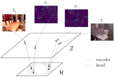
Figure 12: Contrastive learning approach to promote geometric representation. Figure reused from [98]

Shim and Kim [98] focus on learning geometric representation for depth estimation problems using contrastive learning. They utilize Sobel kernel and Canny edge binary mask [101] to generate gradient fields of the image as the positive and negative pairs, see Fig. 12. To estimate the gradient field $G$ ($+$ for positive and $-$ for negative examples) of input image pairs $\mathcal{I}_{q}$ (query image) and $\mathcal{I}_{-}$ (other image), they modify the Canny detector to extract the magnitude of the dominant gradient as well as its location to adjust the gradient field according to its edge dominance. The adopted process can be mathematically formulated as shown in Eq. 72, where $||E||$ and $B_{Canny}$ denote the magnitude of the gradient from the Sobel operator and the binary mask of the Canny detector. $\odot$ is element-wise multiplication.

$$\begin{split}\mathcal{I}&\in\mathbb{R}^{h\times w},\triangledown\mathcal{I}_{x},\triangledown\mathcal{I}_{y}\in\mathbb{R}^{h\times w},\\ ||E||&=\sqrt{\mathcal{I}^{2}_{x}+\mathcal{I}^{2}_{y}},\\ G&=B_{Canny}\odot||E||\end{split}$$ (72)

The network is pre-trained with contrastive loss to learn the geometric representation $\mathcal{Z}$ of the images. This learned representation is further compressed by a 2-layer fully connected network with ReLU non-linear activation to a feature space $\mathcal{H}$. The projected latent vector $h$ of the positive and the negative pairs are used to estimate the contrastive loss.

8 Conclusion

The instrumental progress in deep learning technologies has immensely benefited the depth estimation frameworks. It has enabled the extraction of high-level representations from input images for enhanced stereo matching. However, it has also limited the use of modeling explicit photometric and geometric constraints in the learning process. Most supervised stereo and MVS methods focus on better feature extraction, and enhanced feature matching through attention mechanism but apply a plane-sweep algorithm as the only geometric constraint. They largely depend on the quality of ground truth to learn about geometric and structural consistency in the learning process. In this review, we have comprehensively reviewed geometric concepts in depth estimation and its closely related domains that can be coupled with deep learning frameworks to enforce geometric and structural consistency in the learning process. explicitly modeling geometric constraints, along with the supervision signal, can enforce structural reasoning, occlusion reasoning, and cross-view consistency in a depth estimation framework. We believe this review will provide a good reference for readers and researchers to explore the integration of geometric constraints in deep learning frameworks.

References

- [1] Yasutaka Furukawa and Jean Ponce. Accurate, dense, and robust multiview stereopsis. IEEE Transactions on Pattern Analysis and Machine Intelligence, 32:1362–1376, 2010.
- [2] Silvano Galliani, Katrin Lasinger, and Konrad Schindler. Massively parallel multiview stereopsis by surface normal diffusion. In 2015 IEEE International Conference on Computer Vision (ICCV), pages 873–881, 2015.
- [3] Engin Tola, Christoph Strecha, and Pascal Fua. Efficient large scale multi-view stereo for ultra high resolution image sets. Machine Vision and Applications, 23, 09 2011.
- [4] Johannes L. Schönberger, Enliang Zheng, Jan-Michael Frahm, and Marc Pollefeys. Pixelwise view selection for unstructured multi-view stereo. In Bastian Leibe, Jiri Matas, Nicu Sebe, and Max Welling, editors, Computer Vision – ECCV 2016, pages 501–518, Cham, 2016. Springer International Publishing.
- [5] Yuri Boykov, Olga Veksler, and Ramin Zabih. Fast approximate energy minimization via graph cuts. IEEE Transactions on pattern analysis and machine intelligence, 23:1222–1239, 2001.
- [6] Richard Hartley and Andrew Zisserman. Multiple view geometry in computer vision. Cambridge university press, 2003.
- [7] Quang-Tuan Luong and OD Faugeras. The geometry of multiple images. MIT Press, Boston, 2(3):4–5, 2001.
- [8] Richard Szeliski. Computer vision: algorithms and applications. Springer Nature, 2022.
- [9] Yann LeCun, Yoshua Bengio, and Geoffrey Hinton. Deep learning. nature, 521(7553):436–444, 2015.
- [10] Yann LeCun, Yoshua Bengio, et al. Convolutional networks for images, speech, and time series. The handbook of brain theory and neural networks, 3361(10):1995, 1995.
- [11] Pankaj Malhotra, Lovekesh Vig, Gautam Shroff, Puneet Agarwal, et al. Long short term memory networks for anomaly detection in time series. In Esann, volume 2015, page 89, 2015.
- [12] Alexey Dosovitskiy, Lucas Beyer, Alexander Kolesnikov, Dirk Weissenborn, Xiaohua Zhai, Thomas Unterthiner, Mostafa Dehghani, Matthias Minderer, Georg Heigold, Sylvain Gelly, et al. An image is worth 16x16 words: Transformers for image recognition at scale. arXiv preprint arXiv:2010.11929, 2020.
- [13] Yao Yao, Zixin Luo, Shiwei Li, Tian Fang, and Long Quan. Mvsnet: Depth inference for unstructured multi-view stereo. In Proceedings of the European conference on computer vision (ECCV), pages 767–783, 2018.
- [14] Xiaodong Gu, Zhiwen Fan, Siyu Zhu, Zuozhuo Dai, Feitong Tan, and Ping Tan. Cascade cost volume for high-resolution multi-view stereo and stereo matching. In Proceedings of the IEEE/CVF conference on computer vision and pattern recognition, pages 2495–2504, 2020.
- [15] Yikang Ding, Wentao Yuan, Qingtian Zhu, Haotian Zhang, Xiangyue Liu, Yuanjiang Wang, and Xiao Liu. Transmvsnet: Global context-aware multi-view stereo network with transformers. In Proceedings of the IEEE/CVF Conference on Computer Vision and Pattern Recognition, pages 8585–8594, 2022.
- [16] Alex Kendall, Hayk Martirosyan, Saumitro Dasgupta, Peter Henry, Ryan Kennedy, Abraham Bachrach, and Adam Bry. End-to-end learning of geometry and context for deep stereo regression. In Proceedings of the IEEE international conference on computer vision, pages 66–75, 2017.
- [17] Robert T Collins. A space-sweep approach to true multi-image matching. In Proceedings CVPR IEEE computer society conference on computer vision and pattern recognition, pages 358–363. Ieee, 1996.
- [18] Hongbin Xu, Zhipeng Zhou, Yu Qiao, Wenxiong Kang, and Qiuxia Wu. Self-supervised multi-view stereo via effective co-segmentation and data-augmentation. In Proceedings of the AAAI Conference on Artificial Intelligence, volume 35, pages 3030–3038, 2021.
- [19] Ravi Garg, Vijay Kumar Bg, Gustavo Carneiro, and Ian Reid. Unsupervised cnn for single view depth estimation: Geometry to the rescue. In Computer Vision–ECCV 2016: 14th European Conference, Amsterdam, The Netherlands, October 11-14, 2016, Proceedings, Part VIII 14, pages 740–756. Springer, 2016.
- [20] Zhenheng Yang, Peng Wang, Wei Xu, Liang Zhao, and Ramakant Nevatia. Unsupervised learning of geometry with edge-aware depth-normal consistency. arXiv preprint arXiv:1711.03665, 2017.
- [21] Jiayu Yang, Jose M Alvarez, and Miaomiao Liu. Self-supervised learning of depth inference for multi-view stereo. In Proceedings of the IEEE/CVF Conference on Computer Vision and Pattern Recognition, pages 7526–7534, 2021.
- [22] Baichuan Huang, Hongwei Yi, Can Huang, Yijia He, Jingbin Liu, and Xiao Liu. M3vsnet: Unsupervised multi-metric multi-view stereo network. In 2021 IEEE International Conference on Image Processing (ICIP), pages 3163–3167. IEEE, 2021.
- [23] Yuhua Chen, Cordelia Schmid, and Cristian Sminchisescu. Self-supervised learning with geometric constraints in monocular video: Connecting flow, depth, and camera. In Proceedings of the IEEE/CVF International Conference on Computer Vision, pages 7063–7072, 2019.
- [24] Jingchun Cheng, Yi-Hsuan Tsai, Shengjin Wang, and Ming-Hsuan Yang. Segflow: Joint learning for video object segmentation and optical flow. In Proceedings of the IEEE international conference on computer vision, pages 686–695, 2017.
- [25] Reza Mahjourian, Martin Wicke, and Anelia Angelova. Unsupervised learning of depth and ego-motion from monocular video using 3d geometric constraints. In Proceedings of the IEEE conference on computer vision and pattern recognition, pages 5667–5675, 2018.
- [26] Clément Godard, Oisin Mac Aodha, and Gabriel J Brostow. Unsupervised monocular depth estimation with left-right consistency. In Proceedings of the IEEE conference on computer vision and pattern recognition, pages 270–279, 2017.
- [27] David Eigen and Rob Fergus. Predicting depth, surface normals and semantic labels with a common multi-scale convolutional architecture. In Proceedings of the IEEE international conference on computer vision, pages 2650–2658, 2015.
- [28] Pier Luigi Dovesi, Matteo Poggi, Lorenzo Andraghetti, Miquel Martí, Hedvig Kjellström, Alessandro Pieropan, and Stefano Mattoccia. Real-time semantic stereo matching. In 2020 IEEE international conference on robotics and automation (ICRA), pages 10780–10787. IEEE, 2020.
- [29] Guorun Yang, Hengshuang Zhao, Jianping Shi, Zhidong Deng, and Jiaya Jia. Segstereo: Exploiting semantic information for disparity estimation. In Proceedings of the European conference on computer vision (ECCV), pages 636–651, 2018.
- [30] Taher Naderi, Amir Sadovnik, Jason Hayward, and Hairong Qi. Monocular depth estimation with adaptive geometric attention. In Proceedings of the IEEE/CVF Winter Conference on Applications of Computer Vision, pages 944–954, 2022.
- [31] Zuria Bauer, Zuoyue Li, Sergio Orts-Escolano, Miguel Cazorla, Marc Pollefeys, and Martin R Oswald. Nvs-monodepth: Improving monocular depth prediction with novel view synthesis. In 2021 International Conference on 3D Vision (3DV), pages 848–858. IEEE, 2021.
- [32] Qingtian Zhu, Chen Min, Zizhuang Wei, Yisong Chen, and Guoping Wang. Deep learning for multi-view stereo via plane sweep: A survey. arXiv preprint arXiv:2106.15328, 2021.
- [33] N.A. Wikipedia article: Photogrammetry. In Wikipedia, Accessed: 2023-10-12.
- [34] Richard Szeliski and Polina Golland. Stereo matching with transparency and matting. In Sixth International Conference on Computer Vision (IEEE Cat. No. 98CH36271), pages 517–524. IEEE, 1998.
- [35] Hideo Saito and Takeo Kanade. Shape reconstruction in projective grid space from large number of images. In Proceedings. 1999 IEEE Computer Society Conference on Computer Vision and Pattern Recognition (Cat. No PR00149), volume 2, pages 49–54. IEEE, 1999.
- [36] Yao Yao, Zixin Luo, Shiwei Li, Tianwei Shen, Tian Fang, and Long Quan. Recurrent mvsnet for high-resolution multi-view stereo depth inference. Computer Vision and Pattern Recognition (CVPR), 2019.
- [37] Bo Peng, Eric Alcaide, Quentin Anthony, Alon Albalak, Samuel Arcadinho, Huanqi Cao, Xin Cheng, Michael Chung, Matteo Grella, Kranthi Kiran GV, et al. Rwkv: Reinventing rnns for the transformer era. arXiv preprint arXiv:2305.13048, 2023.
- [38] Po-Han Huang, Kevin Matzen, Johannes Kopf, Narendra Ahuja, and Jia-Bin Huang. Deepmvs: Learning multi-view stereopsis. In Proceedings of the IEEE Conference on Computer Vision and Pattern Recognition, pages 2821–2830, 2018.
- [39] Olaf Ronneberger, Philipp Fischer, and Thomas Brox. U-net: Convolutional networks for biomedical image segmentation. In Medical Image Computing and Computer-Assisted Intervention–MICCAI 2015: 18th International Conference, Munich, Germany, October 5-9, 2015, Proceedings, Part III 18, pages 234–241. Springer, 2015.
- [40] Jiayu Yang, Wei Mao, Jose M Alvarez, and Miaomiao Liu. Cost volume pyramid based depth inference for multi-view stereo. In Proceedings of the IEEE/CVF Conference on Computer Vision and Pattern Recognition, pages 4877–4886, 2020.
- [41] David Gallup, Jan-Michael Frahm, Philippos Mordohai, Qingxiong Yang, and Marc Pollefeys. Real-time plane-sweeping stereo with multiple sweeping directions. In 2007 IEEE Conference on Computer Vision and Pattern Recognition, pages 1–8. IEEE, 2007.
- [42] Dorothy M Greig, Bruce T Porteous, and Allan H Seheult. Exact maximum a posteriori estimation for binary images. Journal of the Royal Statistical Society Series B: Statistical Methodology, 51:271–279, 1989.
- [43] Christopher M Bishop and Nasser M Nasrabadi. Pattern recognition and machine learning, volume 4. Springer, 2006.
- [44] Arijit Mallick, Jörg Stückler, and Hendrik Lensch. Learning to adapt multi-view stereo by self-supervision. arXiv preprint arXiv:2009.13278, 2020.
- [45] Haimei Zhao, Jing Zhang, Zhuo Chen, Bo Yuan, and Dacheng Tao. On robust cross-view consistency in self-supervised monocular depth estimation. arXiv preprint arXiv:2209.08747, 2022.
- [46] Hongbin Xu, Zhipeng Zhou, Yali Wang, Wenxiong Kang, Baigui Sun, Hao Li, and Yu Qiao. Digging into uncertainty in self-supervised multi-view stereo. In Proceedings of the IEEE/CVF International Conference on Computer Vision, pages 6078–6087, 2021.
- [47] Liman Liu, Fenghao Zhang, Wanjuan Su, Yuhang Qi, and Wenbing Tao. Geometric prior-guided self-supervised learning for multi-view stereo. Remote Sensing, 15(8):2109, 2023.
- [48] Tejas Khot, Shubham Agrawal, Shubham Tulsiani, Christoph Mertz, Simon Lucey, and Martial Hebert. Learning unsupervised multi-view stereopsis via robust photometric consistency. arXiv preprint arXiv:1905.02706, 2019.
- [49] Jingliang Li, Zhengda Lu, Yiqun Wang, Ying Wang, and Jun Xiao. Ds-mvsnet: Unsupervised multi-view stereo via depth synthesis. In Proceedings of the 30th ACM International Conference on Multimedia, pages 5593–5601, 2022.
- [50] Haonan Dong and Jian Yao. Patchmvsnet: Patch-wise unsupervised multi-view stereo for weakly-textured surface reconstruction. arXiv preprint arXiv:2203.02156, 2022.
- [51] Hongbin Xu, Zhipeng Zhou, Weitao Chen, Baigui Sun, Hao Li, and Wenxiong Kang. Semi-supervised deep multi-view stereo. arXiv preprint arXiv:2207.11699, 2022.
- [52] Zehao Yu, Lei Jin, and Shenghua Gao. P 2 net: Patch-match and plane-regularization for unsupervised indoor depth estimation. In European Conference on Computer Vision, pages 206–222. Springer, 2020.
- [53] Jakob Engel, Vladlen Koltun, and Daniel Cremers. Direct sparse odometry. IEEE Transactions on Pattern Analysis and Machine Intelligence, 40(3):611–625, 2018.
- [54] Yuchao Dai, Zhidong Zhu, Zhibo Rao, and Bo Li. Mvs2: Deep unsupervised multi-view stereo with multi-view symmetry. In 2019 International Conference on 3D Vision (3DV), pages 1–8. Ieee, 2019.
- [55] Shu Chen, Zhengdong Pu, Xiang Fan, and Beiji Zou. Fixing defect of photometric loss for self-supervised monocular depth estimation. IEEE Transactions on Circuits and Systems for Video Technology, 32(3):1328–1338, 2021.
- [56] Liang Liu, Jiangning Zhang, Ruifei He, Yong Liu, Yabiao Wang, Ying Tai, Donghao Luo, Chengjie Wang, Jilin Li, and Feiyue Huang. Learning by analogy: Reliable supervision from transformations for unsupervised optical flow estimation. In 2020 IEEE/CVF Conference on Computer Vision and Pattern Recognition (CVPR), pages 6488–6497, 2020.
- [57] Simon Meister, Junhwa Hur, and Stefan Roth. Unflow: Unsupervised learning of optical flow with a bidirectional census loss. In Proceedings of the AAAI conference on artificial intelligence, volume 32, 2018.
- [58] Clément Godard, Oisin Mac Aodha, Michael Firman, and Gabriel J Brostow. Digging into self-supervised monocular depth estimation. In Proceedings of the IEEE/CVF international conference on computer vision, pages 3828–3838, 2019.
- [59] Rui Chen, Songfang Han, Jing Xu, and Hao Su. Point-based multi-view stereo network. In Proceedings of the IEEE/CVF international conference on computer vision, pages 1538–1547, 2019.
- [60] Zhou Wang, Alan C Bovik, Hamid R Sheikh, and Eero P Simoncelli. Image quality assessment: from error visibility to structural similarity. IEEE transactions on image processing, 13(4):600–612, 2004.
- [61] A.M. Eskicioglu and P.S. Fisher. Image quality measures and their performance. IEEE Transactions on Communications, 43(12):2959–2965, 1995.
- [62] Hang Zhao, Orazio Gallo, Iuri Frosio, and Jan Kautz. Loss functions for neural networks for image processing. arXiv preprint arXiv:1511.08861, 2015.
- [63] Kaixuan Wang, Yao Chen, Hengkai Guo, Linfu Wen, and Shaojie Shen. Geometric pretraining for monocular depth estimation. In 2020 IEEE International Conference on Robotics and Automation (ICRA), pages 4782–4788. IEEE, 2020.
- [64] Zhichao Yin and Jianping Shi. Geonet: Unsupervised learning of dense depth, optical flow and camera pose. In Proceedings of the IEEE Conference on Computer Vision and Pattern Recognition (CVPR), June 2018.
- [65] Shanshan Zhao, Huan Fu, Mingming Gong, and Dacheng Tao. Geometry-aware symmetric domain adaptation for monocular depth estimation. In Proceedings of the IEEE/CVF Conference on Computer Vision and Pattern Recognition, pages 9788–9798, 2019.
- [66] Sergio Uras, Federico Girosi, Alessandro Verri, and Vincent Torre. A computational approach to motion perception. Biological cybernetics, 60:79–87, 1988.
- [67] Thomas Brox, Andrés Bruhn, Nils Papenberg, and Joachim Weickert. High accuracy optical flow estimation based on a theory for warping. In Computer Vision-ECCV 2004: 8th European Conference on Computer Vision, Prague, Czech Republic, May 11-14, 2004. Proceedings, Part IV 8, pages 25–36. Springer, 2004.
- [68] Yongming Yang, Shuwei Shao, Tao Yang, Peng Wang, Zhuo Yang, Chengdong Wu, and Hao Liu. A geometry-aware deep network for depth estimation in monocular endoscopy. Engineering Applications of Artificial Intelligence, 122:105989, 2023.
- [69] Junjie Hu, Mete Ozay, Yan Zhang, and Takayuki Okatani. Revisiting single image depth estimation: Toward higher resolution maps with accurate object boundaries. In 2019 IEEE Winter Conference on Applications of Computer Vision (WACV), pages 1043–1051, 2019.
- [70] Christopher Zach, Thomas Pock, and Horst Bischof. A duality based approach for realtime tv-l 1 optical flow. In Pattern Recognition: 29th DAGM Symposium, Heidelberg, Germany, September 12-14, 2007. Proceedings 29, pages 214–223. Springer, 2007.
- [71] Pedro F Felzenszwalb and Daniel P Huttenlocher. Efficient graph-based image segmentation. International journal of computer vision, 59:167–181, 2004.
- [72] Paul J Besl and Neil D McKay. Method for registration of 3-d shapes. In Sensor fusion IV: control paradigms and data structures, volume 1611, pages 586–606. Spie, 1992.
- [73] Y. Chen and G. Medioni. Object modeling by registration of multiple range images. In Proceedings. 1991 IEEE International Conference on Robotics and Automation, pages 2724–2729 vol.3, 1991.
- [74] S. Rusinkiewicz and M. Levoy. Efficient variants of the icp algorithm. In Proceedings Third International Conference on 3-D Digital Imaging and Modeling, pages 145–152, 2001.
- [75] Peng Wang, Xiaohui Shen, Bryan Russell, Scott Cohen, Brian Price, and Alan L Yuille. Surge: Surface regularized geometry estimation from a single image. Advances in Neural Information Processing Systems, 29, 2016.
- [76] Wei Yin, Yifan Liu, Chunhua Shen, and Youliang Yan. Enforcing geometric constraints of virtual normal for depth prediction. In Proceedings of the IEEE/CVF International Conference on Computer Vision, pages 5684–5693, 2019.
- [77] Nathan Silberman, Derek Hoiem, Pushmeet Kohli, and Rob Fergus. Indoor segmentation and support inference from rgbd images. In Computer Vision–ECCV 2012: 12th European Conference on Computer Vision, Florence, Italy, October 7-13, 2012, Proceedings, Part V 12, pages 746–760. Springer, 2012.
- [78] Xiaojuan Qi, Renjie Liao, Zhengzhe Liu, Raquel Urtasun, and Jiaya Jia. Geonet: Geometric neural network for joint depth and surface normal estimation. In Proceedings of the IEEE Conference on Computer Vision and Pattern Recognition, pages 283–291, 2018.
- [79] David F Fouhey, Abhinav Gupta, and Martial Hebert. Data-driven 3d primitives for single image understanding. In Proceedings of the IEEE International Conference on Computer Vision, pages 3392–3399, 2013.
- [80] Uday Kusupati, Shuo Cheng, Rui Chen, and Hao Su. Normal assisted stereo depth estimation. In Proceedings of the IEEE/CVF Conference on Computer Vision and Pattern Recognition, pages 2189–2199, 2020.
- [81] Jiaming Sun, Zehong Shen, Yuang Wang, Hujun Bao, and Xiaowei Zhou. Loftr: Detector-free local feature matching with transformers. In Proceedings of the IEEE/CVF conference on computer vision and pattern recognition, pages 8922–8931, 2021.
- [82] Patrick Ruhkamp, Daoyi Gao, Hanzhi Chen, Nassir Navab, and Beniamin Busam. Attention meets geometry: Geometry guided spatial-temporal attention for consistent self-supervised monocular depth estimation. In 2021 International Conference on 3D Vision (3DV), pages 837–847. IEEE, 2021.
- [83] Jie Zhu, Bo Peng, Wanqing Li, Haifeng Shen, Zhe Zhang, and Jianjun Lei. Multi-view stereo with transformer. arXiv preprint arXiv:2112.00336, 2021.
- [84] Longteng Guo, Jing Liu, Xinxin Zhu, Peng Yao, Shichen Lu, and Hanqing Lu. Normalized and geometry-aware self-attention network for image captioning. In Proceedings of the IEEE/CVF conference on computer vision and pattern recognition, pages 10327–10336, 2020.
- [85] Karen Simonyan and Andrew Zisserman. Very deep convolutional networks for large-scale image recognition. arXiv preprint arXiv:1409.1556, 2014.
- [86] Christian Szegedy, Sergey Ioffe, Vincent Vanhoucke, and Alexander Alemi. Inception-v4, inception-resnet and the impact of residual connections on learning. In Proceedings of the AAAI conference on artificial intelligence, volume 31, 2017.
- [87] Kaiming He, Xiangyu Zhang, Shaoqing Ren, and Jian Sun. Deep residual learning for image recognition. In Proceedings of the IEEE conference on computer vision and pattern recognition, pages 770–778, 2016.
- [88] Justin Johnson, Alexandre Alahi, and Li Fei-Fei. Perceptual losses for real-time style transfer and super-resolution. In Computer Vision–ECCV 2016: 14th European Conference, Amsterdam, The Netherlands, October 11-14, 2016, Proceedings, Part II 14, pages 694–711. Springer, 2016.
- [89] Michael Kazhdan and Hugues Hoppe. Screened poisson surface reconstruction. ACM Transactions on Graphics (ToG), 32(3):1–13, 2013.
- [90] Johannes L Schonberger and Jan-Michael Frahm. Structure-from-motion revisited. In Proceedings of the IEEE conference on computer vision and pattern recognition, pages 4104–4113, 2016.
- [91] Johannes L Schönberger, Enliang Zheng, Jan-Michael Frahm, and Marc Pollefeys. Pixelwise view selection for unstructured multi-view stereo. In Computer Vision–ECCV 2016: 14th European Conference, Amsterdam, The Netherlands, October 11-14, 2016, Proceedings, Part III 14, pages 501–518. Springer, 2016.
- [92] Connor Shorten and Taghi M Khoshgoftaar. A survey on image data augmentation for deep learning. Journal of big data, 6(1):1–48, 2019.
- [93] Armand Joulin, Francis Bach, and Jean Ponce. Multi-class cosegmentation. In 2012 IEEE conference on computer vision and pattern recognition, pages 542–549. IEEE, 2012.
- [94] Vincent Casser, Soeren Pirk, Reza Mahjourian, and Anelia Angelova. Unsupervised monocular depth and ego-motion learning with structure and semantics. In Proceedings of the IEEE/CVF Conference on Computer Vision and Pattern Recognition Workshops, pages 0–0, 2019.
- [95] Chris Ding, Xiaofeng He, and Horst D Simon. On the equivalence of nonnegative matrix factorization and spectral clustering. In Proceedings of the 2005 SIAM international conference on data mining, pages 606–610. SIAM, 2005.
- [96] Edo Collins, Radhakrishna Achanta, and Sabine Susstrunk. Deep feature factorization for concept discovery. In Proceedings of the European Conference on Computer Vision (ECCV), pages 336–352, 2018.
- [97] Raia Hadsell, Sumit Chopra, and Yann LeCun. Dimensionality reduction by learning an invariant mapping. In 2006 IEEE computer society conference on computer vision and pattern recognition (CVPR’06), volume 2, pages 1735–1742. IEEE, 2006.
- [98] Dongseok Shim and H Jin Kim. Learning a geometric representation for data-efficient depth estimation via gradient field and contrastive loss. In 2021 IEEE International Conference on Robotics and Automation (ICRA), pages 13634–13640. IEEE, 2021.
- [99] Seokju Lee, Francois Rameau, Fei Pan, and In So Kweon. Attentive and contrastive learning for joint depth and motion field estimation. In Proceedings of the IEEE/CVF International Conference on Computer Vision, pages 4862–4871, 2021.
- [100] Rizhao Fan, Matteo Poggi, and Stefano Mattoccia. Contrastive learning for depth prediction. In Proceedings of the IEEE/CVF Conference on Computer Vision and Pattern Recognition, pages 3225–3236, 2023.
- [101] John Canny. A computational approach to edge detection. IEEE Transactions on pattern analysis and machine intelligence, 6:679–698, 1986.