Transfer in Sequential Multi-armed Bandits via Reward Samples

Abstract

We consider a sequential stochastic multi-armed bandit problem where the agent interacts with bandit over multiple episodes. The reward distribution of the arms remain constant throughout an episode but can change over different episodes. We propose an algorithm based on UCB to transfer the reward samples from the previous episodes and improve the cumulative regret performance over all the episodes. We provide regret analysis and empirical results for our algorithm, which show significant improvement over the standard UCB algorithm without transfer.

I INTRODUCTION

The Multi-armed Bandit (MAB) problem [1, 2, 3] is a popular sequential decision-making problem where an agent interacts with the environment by taking actions at every time step and in return gets a random reward. The goal of the agent is to maximize the average reward received. Recently, there has been a lot of interest in the application of the MAB problem in the context of online advertisements and recommender systems[4, 5]. One of the problems highlighted in [5] is the user cold start problem, which is the inability of a recommender system to make a good recommendation for a new user in absence of any prior information. In this scenario, it is useful to transfer knowledge from other related users in order to make better initial recommendations to the new user. In the context of a MAB problem, transfer learning uses knowledge from one bandit problem in order to improve the performance of another related bandit problem [6, 7]. In particular, it helps to accelerate learning and make better decisions quickly.

In this paper, we consider a sequential stochastic MAB problem where the agent interacts with the environment sequentially in episodes (similar to [6]), where different episodes are synonymous with different tasks or different bandit problems. The reward distributions of the arms remain constant throughout the episode but change over different episodes. This scenario is useful, for instance, in recommender systems where the reward distributions of recommended items change in order to capture the changing user preferences over time. The goal is to leverage the knowledge from previous episodes in order to improve the performance in the current episode, thereby leading to an overall performance improvement. Towards this, we use reward samples from previous episodes to make decisions in the current episode. Our algorithm is based on the UCB algorithm for bandits [8].

Related Work: Transfer learning in the context of MAB has been studied in the framework of Multi-task learning [6, 9, 10, 11] and Meta-learning [12, 13, 14]. In Multi-task learning, the set of tasks are fixed and they are repeatedly encountered by the learning algorithm whereas in meta-learning, the algorithm learns to adapt to a new task after learning from a few tasks drawn from the same task distribution. For instance, the authors in [6] consider a finite set of bandit problems which are encountered repeatedly over time. In contrast, we consider an infinite set of bandit problems but assume that the problems are “similar” (we define the notion of “similarity” later). The idea of transferring knowledge using samples is used in the SW-UCB algorithm in [15], but it suffers from the notion of negative transfer, where knowledge transfer can degrade the performance. In contrast, our algorithm facilitates knowledge transfer while guaranteeing that there is no negative transfer.

The main contributions of the paper are:
(i) We develop an algorithm based on UCB to transfer knowledge using the reward samples from the previous episodes in a sequential stochastic MAB setting. Our algorithm has a better performance compared to UCB with no transfer.
(ii) We provide the regret analysis for the proposed algorithm and our regret upper bound explicitly captures the performance improvement due to transfer.
(iii) We show via numerical simulations that our algorithm is able to effectively transfer knowledge from previous episodes.

Notations: $\mathds{1}\{E\}$ denotes the indicator function whose value is $1$ if the event (condition) $E$ is true, and $0$ otherwise. $\emptyset$ denotes null set.

II PRELIMINARIES AND PROBLEM STATEMENT

We consider the Multi-Armed Bandit problem with $K$ arms and $J$ episodes. The length of each episode is $n$. Define $[K]\triangleq\{1,2,\cdots,K\}$ and $[J]\triangleq\{1,2,\cdots,J\}$. At any given integer time $t>0$, one among the $K$ arms is pulled and a random reward is received. Let $I_{t}\in[K]$ and $r_{I_{t}}$, denote the arm pulled at time $t$ and the corresponding random reward, respectively. We assume that $r_{I_{t}}\in[0,1]$ and the rewards are independent across time and across all arms. In any given episode, the distributions of the arms do not change. However, they are allowed to be different over different episodes.

Let $\mu_{k}^{j}$ be the mean reward of arm $k$ in episode $j$. Let $\mu^{j}\triangleq[\mu_{1}^{j},\mu_{2}^{j},\cdots,\mu_{K}^{j}]^{T}$ denote the vector containing the mean rewards of all arms for episode $j$. Further, let $k^{j}_{*}\in\mathcal{A}^{j}\triangleq\underset{k\in[K]}{\arg\max}\{\mu_{k}^{j}\}$ and $\mu^{j}_{*}=\max\limits_{k\in[K]}\{\mu_{k}^{j}\}$ denote an optimal arm in episode $j$ and it’s mean reward, respectively. Define $\Delta_{k}^{j}=\mu_{*}^{j}-\mu_{k}^{j}>0$ as the sub-optimality gap of arm $k\notin\mathcal{A}^{j}$ in episode $j$. Note that the mean rewards of the arms are unknown.

We assume that the episodes in the MAB problem are related in the sense that the mean rewards of the arms across episodes do not change considerably. We capture this by the following assumption.

Assumption 1.

We assume that $||\mu^{j_{1}}-\mu^{j_{2}}||_{\infty}\leq\epsilon$ for any $j_{1},j_{2}\in[J]$, where the parameter $0<\epsilon\leq 1$ is assumed to be known.

This assumption implies that for each arm, the mean rewards across all episodes do not differ by more than $\epsilon$. In applications like online advertising and recommender systems, the user preferences change over time only gradually, and therefore, the parameter $\epsilon$ can be used to capture this behaviour.

Let $N_{k}^{j}(t)$ denote the number of pulls of arm $k$ in the time interval $[(j-1)n+1,t]$. Thus, $N_{k}^{j}(t)$ counts the number of times arm $k$ is pulled from the beginning of episode $j$ until time $t$. Note that for episode $j$, the allowable values of $t$ in $N_{k}^{j}(t)$ are $[(j-1)n+1,nj]$. Further, let $S_{k}(t)$ denote the number of pulls of arm $k$ in the time interval $[1,t]$. Thus, $S_{k}(t)$ counts the number of times arm $k$ is pulled from the beginning of episode $1$ until time $t$. For example, if $n=5$ and $j=2$, then $N_{k}^{2}(8)$ counts the number of times arm $k$ is pulled in time instants $6,7,$ and $8$. Further, $S_{k}(8)$ counts the number of times arm $k$ is pulled in the interval $[1,8]$.

The goal of the agent is to decide which arm to pull (what should be the value of $I_{t}$) at any given time $t$ based on the information $\{r_{I_{1}},r_{I_{2}},\cdots,r_{I_{t-1}}\}$ in order to maximize the average reward over all episodes. This is captured by the pseudo-regret $R_{J}$ of the MAB problem over $J$ episodes:

$$R_{J} =\sum\limits_{j=1}^{J}\mathbb{E}\left[\sum\limits_{t=(j-1)n+1}^{jn}(r_{k_{*}^{j}}-r_{I_{t}})\right]$$

$$=\sum\limits_{j=1}^{J}\left(n\mu_{*}^{j}-\mathbb{E}\left[\sum\limits_{t=(j-1)n+1}^{jn}\mu^{j}_{I_{t}}\right]\right)$$

$$=\sum\limits_{j=1}^{J}\sum\limits_{k=1}^{K}\Delta_{k}^{j}\mathbb{E}[N_{k}^{j}(jn)],$$ (1)

where the last equality follows since $\sum_{k=1}^{K}N_{k}^{j}(jn)=n$ for any $j\in[J]$. Thus, the goal is to make decisions $\{I_{t}:1\leq t\leq nJ\}$ to minimize the regret in (II).

In this paper, we exploit the relation among the mean rewards of arms in different episodes (c.f. Assumption 1) in order to minimize the regret $R_{J}$. This is achieved by reusing (transferring) reward samples from previous episodes to make decisions in the current episode. We describe the approach and the proposed algorithm in detail in the next section.

III ALL SAMPLE TRANSFER UCB (AST-UCB)

Our approach of reusing samples from previous episodes builds on the standard UCB algorithm for bandits. In this section, we first describe the UCB algorithm and then our proposed algorithm, which we call All Sample Transfer UCB (AST-UCB).

III-A UCB Algorithm [8]

Intuitively, the arm-pulling decisions should be made on the reward samples obtained from each arm. Since the mean rewards of the arms are unknown, the UCB algorithm computes their sample-average estimates and the corresponding confidence intervals. Then, based on the principle of optimism in the face of uncertainty, the upper (maximum) value in the confidence interval of each arm is treated as the optimistic mean reward of that arm. Then, the arm with the highest optimistic mean reward is pulled.

As time progresses and more reward samples are received, the estimates become better and the confidence intervals become smaller. Thus, the upper value in the confidence interval approaches the true mean. Eventually, the optimistic mean reward of the optimal arm becomes larger than all other sub-optimal arms, and thereafter, only the optimal arm is pulled.

The standard UCB algorithm is used when the arm distributions are assumed to be the same at all times. However, in our setting, the distributions change over episodes. Therefore, one approach would be to implement UCB algorithm separately in each episode by using only the samples of that particular episode. In other words, the UCB algorithm is restarted at the beginning of every episode and it uses only the reward samples received during the current episode. We call this approach as No Transfer UCB (NT-UCB) algorithm. Next, we explain NT-UCB algorithm for episode $j$.

Let $\hat{\mu}_{1k}^{j}(t)$ denote the sample-average estimate of the mean reward of arm $k$ at time $t$, and is computed as:

$$\hat{\mu}_{1k}^{j}(t)=\>\>\frac{\sum\limits_{\tau=(j-1)n+1}^{t}r_{I_{\tau}}\mathds{1}\{I_{\tau}=k\}}{\max\{1,N_{k}^{j}(t)\}},$$ (2)

where $N_{k}^{j}(t)$ denotes the number of times arm $k$ is pulled until time $t$ since the beginning of episode $j$. Next, we compute the optimistic mean reward corresponding to $\hat{\mu}_{1k}^{j}(t)$. For this, we require the following result.

Lemma 1.

Let $\alpha>1$. For episode $j$, time $t\in[(j-1)n+1,jn]$ and arm $k$, with probability at least $1-\frac{2}{(t-(j-1)n)^{\alpha}},$ the following equation is satisfied

$$|\hat{\mu}_{1k}^{j}(t)-\mu_{k}^{j}|\leq p_{1k}^{j}(t)\triangleq\sqrt{\frac{\alpha\log{(t-(j-1)n)}}{2N_{k}^{j}(t)}}.$$ (3)

• The rewards are independent random variables with support $[0,1]$. Using Hoeffding’s inequality[16] for estimate $\hat{\mu}_{1k}^{j}(t)$, we get

  $$\text{Pr}\{|\hat{\mu}_{1k}^{j}(t)-\mu_{k}^{j}|\geq\delta\}\leq 2\exp(-2N_{k}^{j}(t){\delta}^{2}).$$

  Setting $\delta=\sqrt{\frac{\alpha\log(t-(j-1)n)}{2N_{k}^{j}(t)}}$ for $N_{k}^{j}(t)\geq 1$, the lemma follows. ∎

Using Lemma 1, we form a confidence interval for mean reward $\mu_{k}^{j}$ using the estimate $\hat{\mu}_{1k}^{j}(t)$ at time $t$ in episode $j$ as

$$D_{1}^{j}(t)=[\hat{\mu}_{1k}^{j}(t)-p_{1k}^{j}(t),\hat{\mu}_{1k}^{j}(t)+p_{1k}^{j}(t)].$$

Next, the NT-UCB algorithm pulls the arm with maximum optimistic reward:

$$I_{t}=\underset{k\in[K]}{\arg\max}\left\{\hat{\mu}_{1k}^{j}(t-1)+p_{1k}^{j}(t-1)\right\}.$$

The above steps are repeated until the end of episode $j$. Next, we provide an upper bound on the pseudo-regret of the NT-UCB algorithm.

Lemma 2.

Let $\alpha>1$. The pseudo-regret of NT-UCB satisfies

$$R_{J} \leq\sum\limits_{k=1}^{K}\left[2\alpha\log{n}\bigg{(}\sum\limits_{{\begin{subarray}{c}k=1\\ \Delta_{k}^{j}>0\end{subarray}}}^{J}\frac{1}{\Delta_{k}^{j}}\bigg{)}+J_{k}\frac{\alpha+1}{\alpha-1}\right],$$ (4)

$$\text{where}\quad J_{k}=\sum\limits_{k=1}^{J}\Delta_{k}^{j}$$

• An upper bound on the regret over all episodes is obtained by adding the per-episode regret bound of the standard UCB algorithm, which is given as [1]

  $$R_{j}\leq\sum\limits_{{\begin{subarray}{c}k=1\\ \Delta_{k}^{j}>0\end{subarray}}}^{K}\left(\frac{2\alpha\log{n}}{\Delta_{k}^{j}}+\frac{\alpha+1}{\alpha-1}\Delta_{k}^{j}\right).$$

  The result then follows. ∎

III-B AST-UCB Algorithm

For any particular episode, the NT-UCB algorithm mentioned above uses samples only in that episode to compute the estimates. However, as per Assumption 1, the mean rewards across the episodes are related, and therefore, reward samples in previous episodes carry information about the mean reward in the current episode. In order to capture this information, we construct an auxiliary estimate (in addition to the UCB estimate) that uses the reward samples from the beginning of the first episode. Then, we combine these two estimates to make the decisions. Next, we describe this approach for episode $j$.

Let $\hat{\mu}_{2k}(t)$ denote the auxiliary sample-average estimate of the mean reward of arm $k$ at time $t$, computed as:

$$\hat{\mu}_{2k}(t)=\>\frac{\sum\limits_{\tau=1}^{t}r_{I_{\tau}}\mathds{1}\{I_{\tau}=k\}}{\max\{1,S_{k}(t)\}},$$ (5)

where $S_{k}(t)$ denotes the number of times arm $k$ is pulled until time $t$ since the beginning of episode $1$. Note that estimate $\hat{\mu}_{2k}(t)$ captures the information of reward samples of arm $k$ from all previous episodes . Next, we compute the optimistic mean reward corresponding to $\hat{\mu}_{2k}(t)$. For this, we require the following result.

Lemma 3.

Let $\alpha>1$. For episode $j$, time $t\in[(j-1)n+1,jn]$ and arm $k$, with probability at least $1-\frac{2}{(t-(j-1)n)^{\alpha}},$ the following equation is satisfied

$$|\hat{\mu}_{2k}(t) -\mu_{k}^{j}|\leq p_{2k}^{j}(t)\triangleq\sqrt{\frac{\alpha\log{(t-(j-1)n})}{2S_{k}(t)}}+U_{k}^{j}(t)\epsilon,$$ (6)

$$\text{where}\quad U_{k}^{j}(t)=\frac{S_{k}(t)-N_{k}^{j}(t)}{S_{k}(t)}.$$

• The rewards are independent random variables with support $[0,1]$. Using McDiarmid’s inequality[17] for estimate $\hat{\mu}_{2k}(t)$, we get

  $$\text{Pr}\{\lvert\hat{\mu}_{2k}(t)-\mathbb{E}[\hat{\mu}_{2k}(t)]\rvert\geq\delta\}\leq 2\exp(-2S_{k}(t){\delta}^{2}).$$

  Setting $\delta=\sqrt{\frac{\alpha\log((t-(j-1)n))}{2S_{k}(t)}}$ for $S_{k}(t)\geq 1$, we get

  $$\text{Pr}\left\{|\hat{\mu}_{2k}(t)-\mathbb{E}[\hat{\mu}_{2k}(t)]|\geq\sqrt{\frac{\alpha\log(t-(j-1)n)}{2S_{k}(t)}}\right\}$$

  $$\leq\frac{2}{(t-(j-1)n)^{\alpha}}.$$

  Hence, with probability at least $1-\frac{2}{(t-(j-1)n)^{\alpha}}$, the following holds

  $$|\hat{\mu}_{2k}(t)-\mathbb{E}[\hat{\mu}_{2k}(t)]|\leq\sqrt{\frac{\alpha\log(t-(j-1)n)}{2S_{k}(t)}}.$$ (7)

  Next, we bound $\mathbb{E}[\hat{\mu}_{2k}(t)]$ for $S_{k}(t)\geq 1$, $t\in[(j-1)n+1,jn]$:

  $$\mathbb{E}[\hat{\mu}_{2k}(t)] =\frac{\sum\limits_{l=1}^{j-1}N_{k}^{l}(ln)\mu_{k}^{l}+N_{k}^{j}(t)\mu_{k}^{j}}{S_{k}(t)},$$

  $$=\mu_{k}^{j}+\frac{\sum\limits_{l=1}^{j-1}N_{k}^{l}(ln)(\mu_{k}^{l}-\mu_{k}^{j})}{S_{k}(t)},$$

  $$\leq\mu_{k}^{j}+\frac{(S_{k}^{j}(t)-N_{k}^{j}(t))\epsilon}{S_{k}(t)},$$

  $$=\mu_{k}^{j}+U_{k}^{j}(t)\epsilon,$$ (8)

  where the inequality follows from $\mu_{k}^{l}-\mu_{k}^{j}\leq\epsilon$ (Asssumption 1). Similarly, using $\mu_{k}^{l}-\mu_{k}^{j}\geq-\epsilon$ (Asssumption 1), we get

  $$\mathbb{E}[\hat{\mu}_{2k}(t)]\geq\mu_{k}^{j}-U_{k}^{j}(t)\epsilon.$$ (9)

  Conditions (Proof.) and (9) yield $|\mathbb{E}[\hat{\mu}_{2k}(t)]|\leq\mu_{k}^{j}+U_{k}^{j}(t)\epsilon$. Using this in (7), we get the result in (6). ∎

Using Lemma 3, we form a confidence interval for mean reward $\mu_{k}^{j}$ using the estimate $\hat{\mu}_{2k}(t)$ at time step $t$ in episode $j$ as

$$D_{2}^{j}(t)=[\hat{\mu}_{2k}(t)-p_{2k}^{j}(t),\hat{\mu}_{2k}(t)+p_{2k}^{j}(t)].$$

Next, we present two key steps of the AST-UCB algorithm.

(i) Combine the optimistic rewards of the two estimates $\hat{\mu}_{1k}^{j}(t)$ and $\hat{\mu}_{2k}(t)$ given in (2) and (5) as:

$$q_{k}^{j}(t)=\min\{\hat{\mu}_{1k}^{j}(t)+p_{1k}^{j}(t),\hat{\mu}_{2k}(t)+p_{2k}^{j}(t)\}.$$ (10)

(ii) Pull arm

$$I_{t}=\underset{k\in[K]}{\arg\max}\{q_{k}^{j}(t-1)\}.$$

The above steps are repeated until the end of episode $j$. All the steps of AST-UCB are given below in Algorithm 1.

Algorithm 1 AST-UCB

Episode length $n$, Number of episodes $J$, Parameters $\alpha$, $\epsilon$ and Number of arms $K$

for episode $j=1,2,...,J$ do

     for $t=(j-1)n+1,\cdots,(j-1)n+K$ do

         $I_{t}=t-(j-1)n$ (Pull each arm once)

     end for

     for $t=(j-1)n+K+1,\cdots,jn$ do

         compute $\hat{\mu}_{1k}^{j}(t-1)$, $p_{1k}^{j}(t-1)$ using (2),(3)

         compute $\hat{\mu}_{2k}(t-1)$, $p_{2k}^{j}(t-1)$ using (5),(6)

         compute optimistic reward $q_{k}^{j}(t-1)$ using (10)

         select arm $I_{t}=\underset{k\in[K]}{\arg\max}\{q_{k}^{j}(t-1)\}$

         update number of pulls $N_{k}^{j}(t)$ and $S_{k}(t)$

     end for

end for

Next, we explain the motivation for Step (i). We combine the confidence intervals $D_{1k}^{j}(t)$ and $D_{2k}^{j}(t)$ by taking their intersection to get a better confidence interval. Note that by taking the intersection, the new confidence interval $D_{1k}^{j}(t)\cap D_{2k}^{j}(t)$ is always smaller than the original two confidence intervals, as illustrated in Figure 1. This smaller interval results in a better estimate of $\mu_{k}^{j}$. We then pick the optimistic reward in the new confidence interval. Further, Step (ii) is similar to the UCB algorithm where we pull the arm with the maximum optimistic reward. The next result presents a bound on the probability of $\mu_{k}^{j}$ lying in the new confidence interval (the new confidence interval being non-empty).

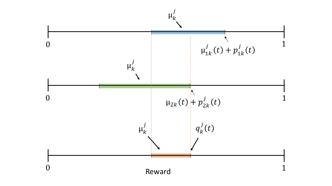
Figure 1: The blue and green intervals represent confidence intervals $D_{1k}^{j}(t)$ and $D_{2k}^{j}(t)$ for mean $\mu_{k}^{j}$, respectively. The orange interval is the intersection of the two intervals, which is clearly smaller (and hence better). The optimistic reward of the orange interval is given by $q_{k}^{j}(t)$.

Lemma 4.

For episode $j$, time $t\in[(j-1)n+1,jn]$ and arm $k$, with probability at least $1-\frac{4}{(t-(j-1)n)^{\alpha}},$ the following equations are satisfied

$$(i)\quad\mu_{k}^{j}\in D_{1k}^{j}(t)\cap D_{2k}^{j}(t).$$ (11)

$$(ii)\quad D_{1k}^{j}(t)\cap D_{2k}^{j}(t)=\emptyset.$$ (12)

• Define events $\mathcal{E}_{1}=\{\mu_{k}^{j}\notin D_{1k}^{j}(t)\}$ and $\mathcal{E}_{2}=\{\mu_{k}^{j}\notin D_{1k}^{j}(t)\}$. Then we have

  $$\text{Pr}\{\mu_{k}^{j}\notin D_{1k}^{j}(t)\cap D_{2k}^{j}(t)\} =\text{Pr}\{\mathcal{E}_{1}\cup\mathcal{E}_{2}\}$$

  $$\leq\text{Pr}\{\mathcal{E}_{1}\}+\text{Pr}\{\mathcal{E}_{2}\}$$

  $$\leq\frac{4}{(t-(j-1)n)^{\alpha}},$$

  where the last inequality follows from Lemmas 1 and 3. Hence, condition (i) in the lemma follows. Same arguments are valid for condition (ii) as well. ∎

Note that although the new confidence interval is smaller, Lemma 4 shows that the probability bound of the mean reward belonging to this new interval has reduced as compared to that in (3) or (6). However, we show in Theorem 1 that the negative effect of the reduction of the probability is not significant, and the smaller interval leads to an overall reduction in the regret.

IV REGRET ANALYSIS

In this section, we derive the regret of the AST-UCB algorithm and then provide the analysis of the result.

Theorem 1.

Let $\Delta_{k}^{max}\triangleq\max\limits_{j\in[J]}\>\{\Delta_{k}^{j}\}$ and $\Delta_{k}^{min}\triangleq\min\limits_{j\in[J],\Delta_{k}^{j}>0}\>\{\Delta_{k}^{j}\}$. The pseudo-regret of AST-UCB with $\alpha>1$ and $0\leq\epsilon<\frac{1}{2}\min\limits_{k\in[K]}\{\Delta_{k}^{min}\}$ satisfies

$$R_{J} \leq\sum\limits_{k=1}^{K}\Delta_{k}^{max}\Bigg{[}\min\bigg{\{}\sum\limits_{\begin{subarray}{c}j=1\\ \Delta_{k}^{j}>0\end{subarray}}^{J}\frac{2\alpha\log{(n)}}{(\Delta_{k}^{j})^{2}},\frac{2\alpha\log{(n)}}{(\Delta_{k}^{\min}-2\epsilon)^{2}}\bigg{\}}$$

$$\hskip 85.35826pt+J\frac{\alpha+3}{\alpha-1}\Bigg{]}.$$ (13)

• Refer to the appendix. ∎

Next, we compare the regret bounds of our algorithm (1) and NT-UCB (4), and highlight the benefit of transfer. The transfer happens due to the first term in (1). Hence, we compare the first terms in the regret bounds. To this end, we define the following terms that capture the dependence on $J$:

$$A_{k}^{J}=\sum\limits_{\begin{subarray}{c}j=1\\ \Delta_{k}^{j}>0\end{subarray}}^{J}\frac{\Delta_{k}^{max}}{(\Delta_{k}^{j})^{2}},B_{k}^{J}=\frac{\Delta_{k}^{max}}{(\Delta_{k}^{\min}-2\epsilon)^{2}},C_{k}^{J}=\sum\limits_{\begin{subarray}{c}j=1\\ \Delta_{k}^{j}>0\end{subarray}}^{J}\frac{1}{\Delta_{k}^{j}}.$$

Several comments are in order. First, observe that, for transfer to be beneficial, we need $\min\{A_{k}^{J},B_{k}^{j}\}<C_{k}^{J}$. Since $A_{k}^{J}\geq C_{k}^{J}$, this can happen only if $B_{k}^{J}<C_{k}^{J}$ . The term $B_{k}^{J}$ behaves like a constant as compared to $C_{k}^{J}$ which increases as the total number of episodes $J$ increases. Therefore, for some large enough $J^{m}(\epsilon)$, we get $C_{k}^{J^{m}(\epsilon)}<B_{k}^{J^{m}(\epsilon)}$ which leads to decrease in the regret as compared to NT-UCB. Second, as $\epsilon$ increases (episodes become increasingly non-related), $J^{m}(\epsilon)$ increases since more episodes (samples) are required for the transfer to be beneficial. Third, we have logarithmic dependence of episode length $n$ on the regret (which is the case with NT-UCB as well). Fourth, the second term in the regret bound of AST-UCB (1) is higher than the corresponding term in NT-UCB bound (4) due to the decreased probability bound in Lemma 4 as compared to Lemmas 1 and 3.

V Numerical Simulations

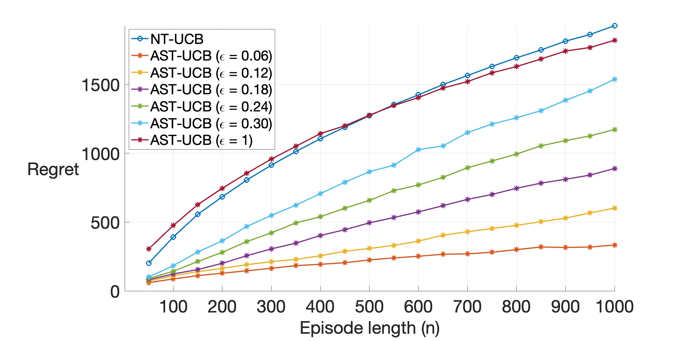
(a) Regret as function of episode length $n$.

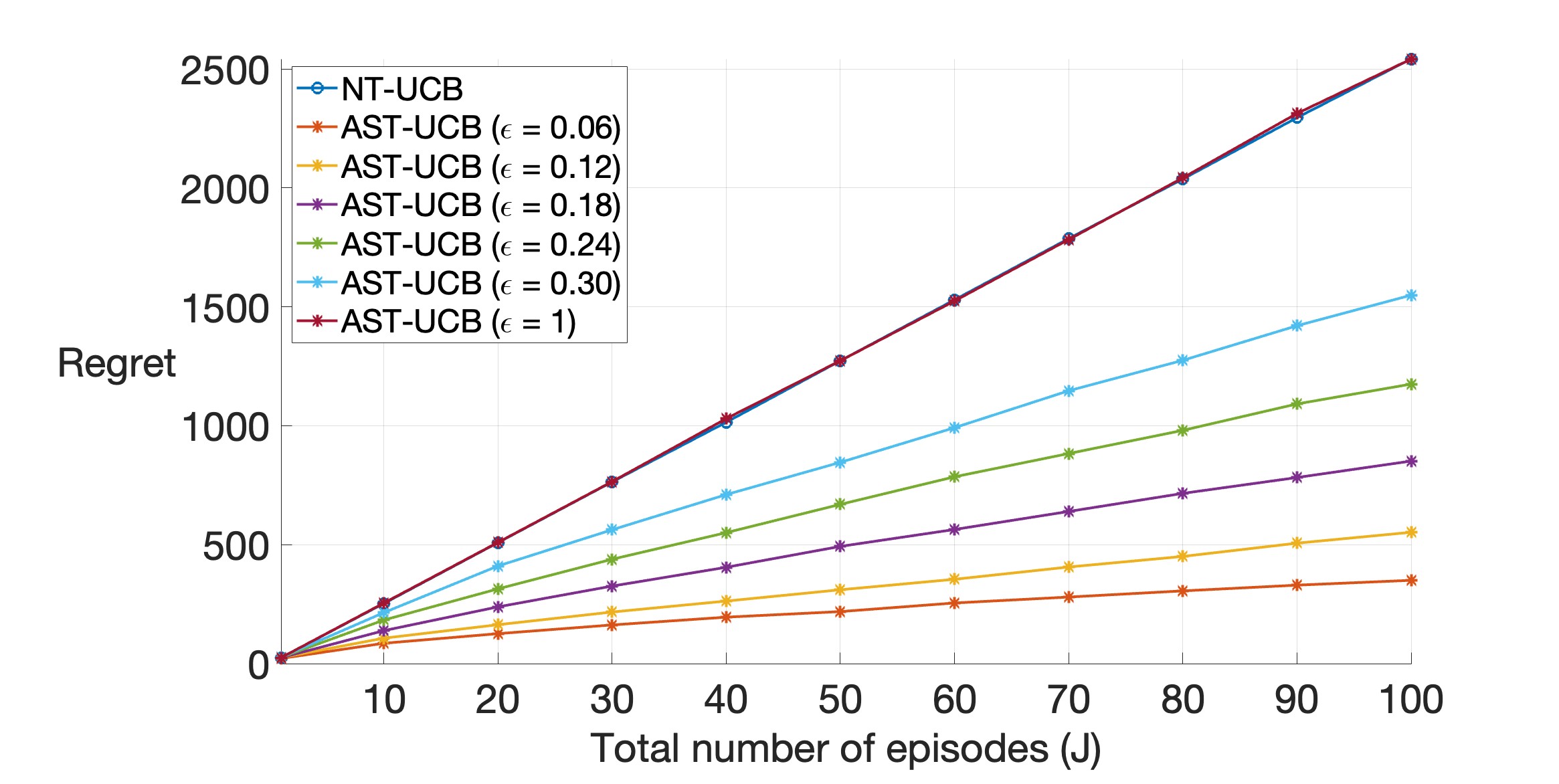
(b) Regret as function of total number of episodes $J$.

Figure 2: Empirical regret of NT-UCB and AST-UCB for different values of $\epsilon$ for Case I.

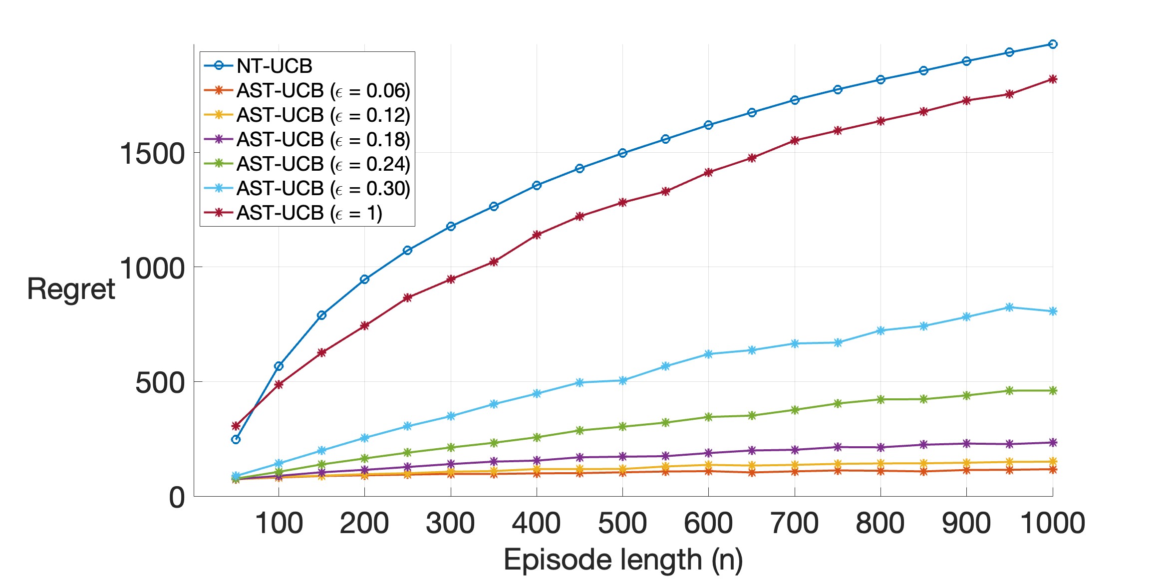
(a) Regret as function of episode length $n$.

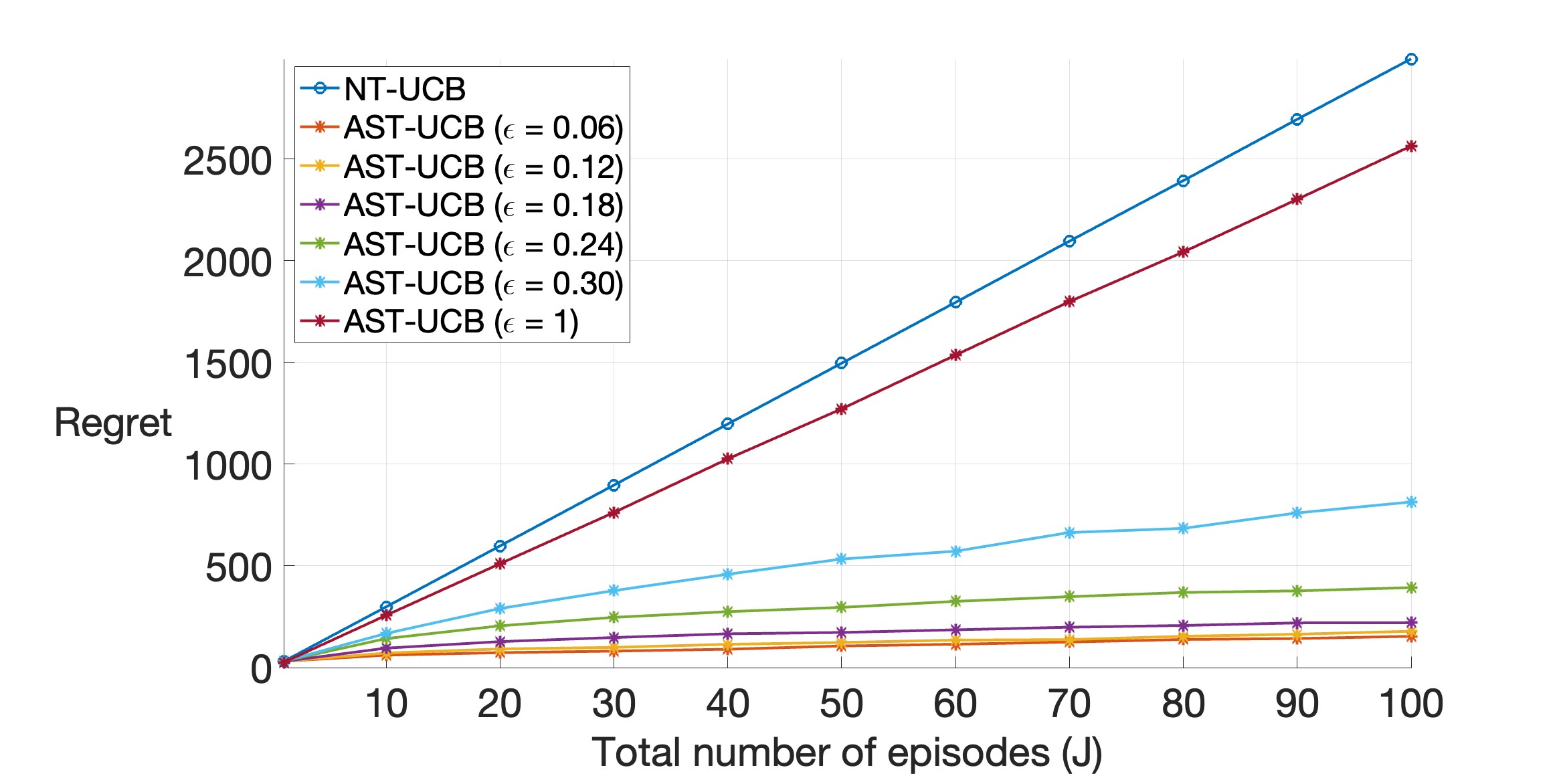
(b) Regret as function of total number of episodes $J$.

Figure 3: Empirical regret of NT-UCB and AST-UCB for different values of $\epsilon$ for Case II.

In this section, we present the numerical results for AST-UCB algorithm. We consider $K=4$ armed bandit problem. In numerical simulations, we need to select the mean reward ($\mu_{k}^{j}$) of each arm for each episode which should satisfy Assumption 1. Towards this end, we fix a seed interval of length $\epsilon$ for each arm. Then, at the beginning of each episode, we uniformly sample the value of $\mu_{k}^{j}$ from this seed interval. This ensures that Assumption 1 is satisfied. Once the mean reward value $\mu_{k}^{j}$ is obtained, we construct a uniform distribution with mean $\mu_{k}^{j}$ and width $d=0.2$. In case the support of this uniform distribution lies outside the interval $[0,1]$, we reduce $d$ to avoid this. The reward samples are then generated from the uniform distribution. For each scenario, we compute the regret $R_{J}$ by taking an empirical average over $30$ independent realizations of that scenario.

We simulate AST-UCB and NT-UCB for two cases (two sets of seed intervals). Note that the seed intervals for each arm are of length $\epsilon$. The mid-points of the seed intervals of the four arms for Case I and Case II are $(0.4,0.6,0.6,0.4)$ and $(0.35,0.7,0.3,0.4)$, respectively.

In Figure 2(a), we observe that the regret of AST-UCB is considerably smaller as compared to NT-UCB. This is particularly true for smaller values of $\epsilon$. As $\epsilon$ increases, the regret of AST-UCB approaches to that of NT-UCB. This is in accordance with the fact that when $\epsilon$ is large, the confidence interval of the auxiliary estimate in (6) is large and transfer is not much beneficial. Further, we observe a logarithmic dependence of the regret on $n$, as quantified by the regret bounds in (4) and (1).

In Figure 2(b), we again observe that AST-UCB performs better than NT-UCB, particularly for small values of $\epsilon$. We also observe that the regret has a “approximate” linear dependence on $J$. The plots in Figures 2 show that for any value of $\epsilon$ the difference between the regret of NT-UCB and AST-UCB increases with episode length ($n$) or total number of episodes ($J$). This is because a larger number of reward samples from previous episodes become available, thereby increasing the transfer.

Similar observations can be seen in Figures 3(a) and 3(b) for Case II. However, the improvement of AST-UCB over NT-UCB in terms of regret is more in Case II as compared to Case I. This happens because the seed intervals in Case II are farther apart, which helps in distinguishing the best arm more quickly using the samples of previous episodes.

VI CONCLUSION

We analyzed the transfer of reward samples in a sequential stochastic multi-armed bandit setting. We proposed a transfer algorithm based on UCB and showed that its regret is lower than UCB with no transfer. We provide regret analysis of our algorithm and validate our approach via numerical experiments. Future research directions include extending the work to the case when the parameter $\epsilon$ is unknown, and studying a similar transfer problem in the context of reinforcement learning.

APPENDIX: Proof of Theorem 1

To simplify the notation, we re-denote several variables as $\mu=\mu_{k}^{j}$, $\mu_{*}=\mu_{*}^{j}$, $\hat{\mu}_{1}=\hat{\mu}_{1k}^{j}(t-1)$, $\hat{\mu}_{1*}=\hat{\mu}_{1k_{*}^{j}}^{j}(t-1)$, $\hat{\mu}_{2}=\hat{\mu}_{2k}(t-1)$, $\hat{\mu}_{2*}=\hat{\mu}_{2k_{*}^{j}}(t-1)$, $t_{j}^{n}=(j-1)n+1$,

$$p_{1}=\sqrt{\frac{\alpha\log{(t-t_{j}^{n})}}{2N_{k}^{j}(t-1)}},p_{1*}=\sqrt{\frac{\alpha\log{(t-t_{j}^{n})}}{2N_{k_{*}^{j}}^{j}(t-1)}},$$

$$p_{2}=\sqrt{\frac{\alpha\log{(t-t_{j}^{n})}}{2S_{k}(t-1)}}+U_{k}^{j}(t)\epsilon,$$

$$p_{2*}=\sqrt{\frac{\alpha\log{(t-t_{j}^{n})}}{2S_{k_{*}^{j}}(t-1)}}+U_{k_{*}}^{j}(t)\epsilon,$$

$$u_{1k}^{j}=\frac{2\alpha\log{(n)}}{(\Delta_{k}^{j})^{2}},u_{2k}^{j}=\frac{2\alpha\log{(n)}}{(\Delta_{k}^{j}-2\epsilon)^{2}}.$$

For arm $k$ to be pulled at time $t$ ($I_{t}=k$), at least one of the following five conditions should be true:

$$\hat{\mu}_{1}-p_{1} >\mu,$$ (14)

$$\hat{\mu}_{1*}+p_{1*} \leq\mu_{*},$$ (15)

$$\hat{\mu}_{2*}+p_{2*} \leq\mu_{*},$$ (16)

$$\hat{\mu}_{2}-p_{2} >\mu,$$ (17)

$$\sqrt{\frac{\alpha\log{n}}{2N_{k}^{j}(t-1)}} >\frac{\Delta_{k}^{j}}{2}\hskip 11.38092pt\text{and}\hskip 11.38092pt\sqrt{\frac{\alpha\log{(n)}}{2S_{k}(t-1)}}+\epsilon>\frac{\Delta_{k}^{j}}{2}.$$ (18)

We show this by contradiction. Assume that none of the conditions in (14)-(17) is true and the first condition in (18) is false. Then, using the fact that $p_{1}<\sqrt{\frac{\alpha\log{n}}{2N_{k}^{j}(t-1)}}$, we have

$$\hat{\mu}_{1*}+p_{1*} >\mu_{*}=\Delta_{k}^{j}+\mu\geq 2p_{1}+\mu\geq\hat{\mu}_{1}+p_{1},$$ (19)

$$\hat{\mu}_{2*}+p_{2*} >\mu_{*}=\Delta_{k}^{j}+\mu\geq 2p_{1}+\mu\geq\hat{\mu}_{1}+p_{1}.$$ (20)

Conditions in (19) and (20) imply

$$\min\{\hat{\mu}_{1*}+p_{1*},\hat{\mu}_{2*}+p_{2*}\}>\hat{\mu}_{1}+p_{1}.$$ (21)

Similarly, when none of the conditions in (14)-(17) is true and the second condition in (18) is false, we get

$$\min\{\hat{\mu}_{1*}+p_{1*},\hat{\mu}_{2*}+p_{2*}\}>\hat{\mu}_{2}+p_{2}.$$ (22)

Thus, at least one of the conditions in (21) and (22) is true, and this yields

$$\min\{\hat{\mu}_{1*}+p_{1*}, \hat{\mu}_{2*}+p_{2*}\}>\min\{\hat{\mu}_{1}+p_{1},\hat{\mu}_{2}+p_{2}\}.$$

The above condition implies that the AST-UCB algorithm will not pull arm $k$, and hence, we have a contradiction. The cumulative regret after $J$ episodes (each with length $n$) is given by

$$R_{J} =\sum\limits_{j=1}^{J}\sum\limits_{k=1}^{K}\Delta_{k}^{j}\mathbb{E}[N_{k}^{j}(jn)],$$

$$\leq\sum\limits_{k=1}^{K}\Delta_{k}^{\max}\mathbb{E}[\tilde{S}_{k}(Jn)],$$

where $\tilde{S}_{k}(Jn)$ is the total number of sub-optimal pulls to arm $k$ over all episodes. Next, we bound the regret by bounding the term $\mathbb{E}[\tilde{S}_{k}(Jn)]$. For an arbitrary sequence $I_{t}$, $t=1,2,\cdots,Jn$, we have

$$\tilde{S}_{k}(Jn) =\sum\limits_{j=1}^{J}\sum\limits_{t=t_{j}^{n}}^{jn}\mathds{1}\{I_{t}=k;k\neq k_{*}^{j}\},$$

$$=\sum\limits_{j=1}^{J}\bigg{(}\mathds{1}\{k\neq k_{*}^{j}\}+\sum\limits_{t=t_{j}^{n}+K}^{jn}\mathds{1}\{I_{t}=k;k\neq k_{*}^{j}\}\bigg{)},$$

$$=\sum\limits_{j=1}^{J}\sum\limits_{t=t_{j}^{n}+K}^{jn}\mathds{1}\{I_{t}=k;k\neq k_{*}^{j};\eqref{eq:cond5}\hskip 2.84544pt\text{is}\hskip 2.84544pt\text{True}\}$$

$$\hskip 14.22636pt+\sum\limits_{j=1}^{J}\bigg{(}\mathds{1}\{k\neq k_{*}^{j}\}+\sum\limits_{t=t_{j}^{n}+K}^{jn}\mathds{1}\{I_{t}=k;k\neq k_{*}^{j};$$

$$\hskip 39.83368pt\eqref{eq:cond5}\hskip 2.84544pt\text{is}\hskip 2.84544pt\text{False}\}\bigg{)}.$$ (23)

$$\text{First term in \eqref{eq:S_k}}=\sum\limits_{j=1}^{J}\sum\limits_{t=t_{j}^{n}+K}^{jn}\mathds{1}\{I_{t}=k,k\neq k_{*}^{j};$$

$$\hskip 85.35826ptN_{k}^{j}(t-1)<u_{1k}^{j},S_{k}(t-1)<u_{2k}^{j}\},$$

$$=\sum\limits_{j=1}^{J}\sum\limits_{t=t_{j}^{n}+K}^{jn}\min\bigg{\{}\mathds{1}\{I_{t}=k,k\neq k_{*}^{t};N_{k}^{j}(t-1)<u_{1k}^{j}\},$$

$$\hskip 28.45274pt\mathds{1}\{I_{t}=k,k\neq k_{*}^{t};S_{k}(t-1)<u_{2k}^{j}\}\bigg{\}},$$

$$\leq\min\bigg{\{}\sum\limits_{j=1}^{J}\sum\limits_{t=t_{j}^{n}+K}^{jn}\mathds{1}\{I_{t}=k,k\neq k_{*}^{t};N_{k}^{j}(t-1)<u_{1k}^{j}\},$$

$$\hskip 28.45274pt\sum\limits_{j=1}^{J}\sum\limits_{t=t_{j}^{n}+K}^{jn}\mathds{1}\{I_{t}=k,k\neq k_{*}^{t};S_{k}(t-1)<u_{2k}^{j}\}\bigg{\}},$$

$$\leq\min\bigg{\{}\sum\limits_{\begin{subarray}{c}j=1\\ \Delta_{k}^{j}>0\end{subarray}}^{J}\frac{2\alpha\log{(n)}}{(\Delta_{k}^{j})^{2}},\sum\limits_{t=1}^{Jn}\mathds{1}\bigg{\{}I_{t}=k,k\neq k_{*}^{t};$$

$$\hskip 28.45274ptS_{k}(t-1)<\frac{2\alpha\log{(n)}}{(\Delta_{k}^{\min}-2\epsilon)^{2}}\bigg{\}}\bigg{\}},$$

$$\leq\min\bigg{\{}\sum\limits_{\begin{subarray}{c}j=1\\ \Delta_{k}^{j}>0\end{subarray}}^{J}\frac{2\alpha\log{(n)}}{(\Delta_{k}^{j})^{2}},\frac{2\alpha\log{(n)}}{(\Delta_{k}^{\min}-2\epsilon)^{2}}\bigg{\}},$$ (24)

$$\text{Second term of \eqref{eq:S_k}}\leq\sum\limits_{j=1}^{J}\bigg{(}1+\sum\limits_{t=t_{j}^{n}+K}^{jn}\mathds{1}\{\eqref{eq:cond1}\hskip 2.84544pt\text{or}\hskip 2.84544pt\eqref{eq:cond2}$$

$$\hskip 113.81102pt\text{or}\hskip 2.84544pt\eqref{eq:cond3}\hskip 2.84544pt\text{or}\hskip 2.84544pt\eqref{eq:cond4}\hskip 2.84544pt\text{is}\hskip 2.84544pt\text{True}\}\bigg{)}.$$ (25)

Using (APPENDIX: Proof of Theorem 1), (APPENDIX: Proof of Theorem 1), (APPENDIX: Proof of Theorem 1) and taking expectation, we get

$$\mathbb{E}[S_{k}(n)] \leq\min\left\{W_{J},V_{J}\right\}+\sum\limits_{j=1}^{J}\bigg{(}1+\sum\limits_{t=t_{j}^{n}+K}^{jn}\text{Pr}\{\eqref{eq:cond1}\hskip 2.84544pt\text{or}$$

$$\hskip 28.45274pt\eqref{eq:cond2}\hskip 2.84544pt\text{or}\hskip 2.84544pt\eqref{eq:cond3}\hskip 2.84544pt\text{or}\hskip 2.84544pt\eqref{eq:cond4}\hskip 2.84544pt\text{is}\hskip 2.84544pt\text{True}\}\bigg{)},$$ (26)

$$\text{where}\hskip 2.84544ptW_{J} =\sum\limits_{\begin{subarray}{c}j=1\\ \Delta_{k}^{j}>0\end{subarray}}^{J}\frac{2\alpha\log{(n)}}{(\Delta_{k}^{j})^{2}}\hskip 2.84544pt\text{and}\hskip 2.84544ptV_{J}=\frac{2\alpha\log{(n)}}{(\Delta_{k}^{\min}-2\epsilon)^{2}}.$$

Next, we bound the probability of the event that at least one of (14) or (15) or (16) or (17) is true. We use the union bound, followed by the application of one-sided Hoeffding’s inequality (steps are similar to the proof of Lemma 1 and 3) to get,

$$\text{Pr}\{\eqref{eq:cond1}\hskip 2.84544pt\text{or}\hskip 2.84544pt\eqref{eq:cond2}\hskip 2.84544pt\text{or}\hskip 2.84544pt\eqref{eq:cond3}\hskip 2.84544pt\text{or}\hskip 2.84544pt\eqref{eq:cond4}\hskip 2.84544pt\text{is}\hskip 2.84544pt\text{True}\}$$

$$\leq\text{Pr}\{\eqref{eq:cond1}\hskip 2.84544pt\text{is}\hskip 2.84544pt\text{True}\}+\text{Pr}\{\eqref{eq:cond2}\hskip 2.84544pt\text{is}\hskip 2.84544pt\text{True}\}+\text{Pr}\{\eqref{eq:cond3}\hskip 2.84544pt\text{is}\hskip 2.84544pt\text{True}\}$$

$$\hskip 14.22636pt+\text{Pr}\{\eqref{eq:cond4}\hskip 2.84544pt\text{is}\hskip 2.84544pt\text{True}\}\},$$

$$\leq\frac{4}{(t-t_{j}^{n})^{\alpha}}.$$ (27)

Using (APPENDIX: Proof of Theorem 1) and (APPENDIX: Proof of Theorem 1), we have

$$\mathbb{E}[\tilde{S}_{k}(n)]\leq\min\left\{W_{J},V_{J}\right\}+\sum\limits_{j=1}^{J}\bigg{(}1+\sum\limits_{t=t_{j}^{n}+K}^{jn}\frac{4}{(t-t_{j}^{n})^{\alpha}}\bigg{)},$$

$$\leq\min\left\{W_{J},V_{J}\right\}+\sum\limits_{j=1}^{J}\bigg{(}1+\int\limits_{s=(j-1)n+K}^{\infty}\frac{4}{(s-t_{j}^{n})^{\alpha}}ds\bigg{)},$$

$$=\min\left\{W_{J},V_{J}\right\}+\sum\limits_{j=1}^{J}\bigg{(}1+\frac{4(K-1)^{1-\alpha}}{\alpha-1}\bigg{)},$$

$$\leq\min\left\{W_{J},V_{J}\right\}+\sum\limits_{j=1}^{J}\bigg{(}1+\frac{4}{\alpha-1}\bigg{)},$$

$$\leq\min\left\{W_{J},V_{J}\right\}+J\frac{\alpha+3}{\alpha-1}.$$

Hence the theorem follows.

References

• [1] S. Bubeck, N. Cesa-Bianchi, et al., “Regret analysis of stochastic and nonstochastic multi-armed bandit problems,” Foundations and Trends® in Machine Learning, vol. 5, no. 1, pp. 1–122, 2012.
• [2] T. Lattimore and C. Szepesvári, Bandit algorithms. Cambridge University Press, 2020.
• [3] H. Robbins, “Some aspects of the sequential design of experiments,” 1952.
• [4] D. Bouneffouf, I. Rish, and C. Aggarwal, “Survey on applications of multi-armed and contextual bandits,” in 2020 IEEE Congress on Evolutionary Computation (CEC), pp. 1–8, 2020.
• [5] N. Silva, H. Werneck, T. Silva, A. C. Pereira, and L. Rocha, “Multi-armed bandits in recommendation systems: A survey of the state-of-the-art and future directions,” Expert Systems with Applications, vol. 197, p. 116669, 2022.
• [6] A. Lazaric, E. Brunskill, et al., “Sequential transfer in multi-armed bandit with finite set of models,” Advances in Neural Information Processing Systems, vol. 26, 2013.
• [7] A. Shilton, S. Gupta, S. Rana, and S. Venkatesh, “Regret bounds for transfer learning in bayesian optimisation,” in Artificial Intelligence and Statistics, pp. 307–315, PMLR, 2017.
• [8] P. Auer, N. Cesa-Bianchi, and P. Fischer, “Finite-time analysis of the multiarmed bandit problem,” Machine learning, vol. 47, pp. 235–256, 2002.
• [9] J. Zhang and E. Bareinboim, “Transfer learning in multi-armed bandit: a causal approach,” in Proceedings of the 16th Conference on Autonomous Agents and MultiAgent Systems, pp. 1778–1780, 2017.
• [10] A. A. Deshmukh, U. Dogan, and C. Scott, “Multi-task learning for contextual bandits,” Advances in Neural Information Processing Systems, vol. 30, 2017.
• [11] B. Liu, Y. Wei, Y. Zhang, Z. Yan, and Q. Yang, “Transferable contextual bandit for cross-domain recommendation,” in Proceedings of the AAAI Conference on Artificial Intelligence, vol. 32, 2018.
• [12] L. Cella, A. Lazaric, and M. Pontil, “Meta-learning with stochastic linear bandits,” in International Conference on Machine Learning, pp. 1360–1370, PMLR, 2020.
• [13] L. Cella and M. Pontil, “Multi-task and meta-learning with sparse linear bandits,” in Uncertainty in Artificial Intelligence, pp. 1692–1702, PMLR, 2021.
• [14] J. Azizi, B. Kveton, M. Ghavamzadeh, and S. Katariya, “Meta-learning for simple regret minimization,” in Proceedings of the AAAI Conference on Artificial Intelligence, vol. 37, pp. 6709–6717, 2023.
• [15] A. Garivier and E. Moulines, “On upper-confidence bound policies for switching bandit problems,” in International Conference on Algorithmic Learning Theory, pp. 174–188, Springer, 2011.
• [16] W. Hoeffding, “Probability inequalities for sums of bounded random variables,” The collected works of Wassily Hoeffding, pp. 409–426, 1994.
• [17] C. McDiarmid et al., “On the method of bounded differences,” Surveys in combinatorics, vol. 141, no. 1, pp. 148–188, 1989.