Vibrational Polaritons with Broken In-Plane Translational Symmetry

Abstract

For the calculation of polariton dispersion relations in planar Fabry–Pérot microcavities, the single-mode approximation is usually applied. This approximation becomes invalid when the molecular distribution along the cavity mirror plane breaks the in-plane translational symmetry. Herein, both perturbative theory and numerical calculations have been performed to study polariton dispersion relations with various in-plane molecular distribution patterns under vibrational strong coupling conditions. If a homogeneous in-plane molecular distribution is modulated by sinusoidal fluctuations, in addition to a pair of upper and lower polariton branches, a discrete number of side polariton branches may emerge in the polariton dispersion relation. Moreover, for a Gaussian molecular density distribution, only two, yet significantly broadened polariton branches exist in the spectra. This polariton linewidth broadening is due to the breakdown of the single-mode approximation and the scattering between cavity modes at different in-plane frequencies, which is distinguished from known causes of polariton broadening such as the homogeneous broadening of molecules and the cavity loss. Associated with the broadened polariton branches, under the Gaussian in-plane inhomogeneity, a significant amount of the VSC eigenstates contain a non-zero contribution from the cavity photon mode at zero in-plane frequency, blurring the distinction between the bright and the dark modes. Looking forward, our theoretical investigation should facilitate the experimental exploration of vibrational polaritons with patterned in-plane molecular density distributions.

I Introduction

Polaritons, hybrid light-matter states stemming from strong light-matter interactions, have been demonstrated across a wide range of experimental devices [1, 2, 3, 4, 5, 6, 7, 8, 9]. Among different categories of the experimental devices, perhaps the most popular one is a planar Fabry–Pérot microcavity, in which a layer of molecules is confined between a pair of parallel mirrors [10, 11]. For this planar cavity geometry, as shown in Fig. 1, a continuum of cavity modes with the wave vector $\mathbf{k}=(\mathbf{k}_{\parallel},k_{\perp})$ is supported, where $\mathbf{k}_{\parallel}$ denotes an arbitrary in-plane wave vector oriented along the cavity mirror plane, and the discrete perpendicular wave vector $k_{\perp}=m\pi/L_{z}$ (with $m=1,2,\cdots$) is determined by the cavity length $L_{z}$.

When theoretical models are used to describe the polariton dispersion relation (i.e., polariton spectra as a function of $\mathbf{k}_{\parallel}$) in a planar Fabry–Pérot microcavity, the single-mode approximation is usually applied [10]. With this approximation, the molecules are assumed to interact with only a single or a few cavity modes at a specific $\mathbf{k}_{\parallel}$ value. The polariton dispersion relation is then evaluated by independently calculating the polariton eigenstates between the molecules and the cavity mode(s) at each individual $\mathbf{k}_{\parallel}$ value [10].

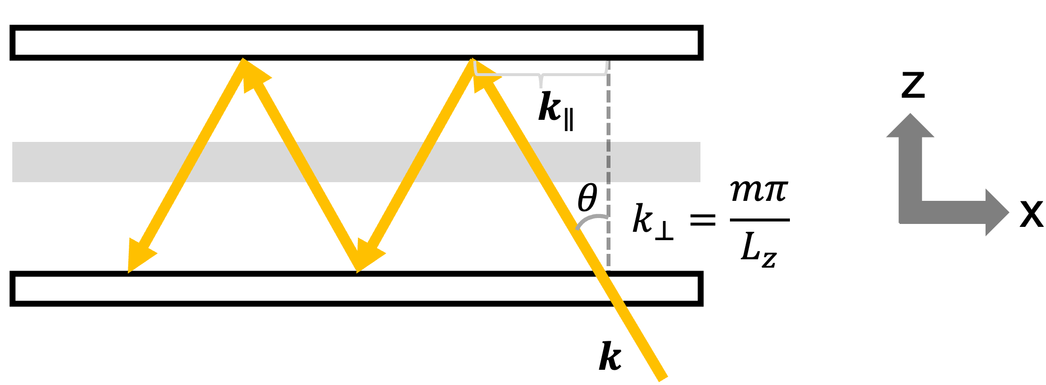
Figure 1: Sketch of a planar Fabry–Pérot microcavity. In this cavity setup, a pair of parallel cavity mirrors is placed along the $z$-direction with a separation of $L_{z}$, and the cavity mirrors span over the $xy$-plane. This cavity supports cavity photon modes with the wave vector $\mathbf{k}=(\mathbf{k}_{\parallel},k_{\perp})$, where the in-plane wave vector $\mathbf{k}_{\parallel}$ is an arbitrary two-dimensional vector in the $xy$-plane, and $k_{\perp}=m\pi/L_{z}$ with $m=1,2,\cdots$. A layer of molecules (gray) is placed at the middle of the cavity to form collective strong coupling with the cavity photon modes.

The validity of the single-mode approximation stems from the translational symmetry of the molecules along the cavity mirror plane [12], an assumption which is usually taken for granted. With this molecular in-plane translational symmetry, when the polariton dispersion relation is evaluated, the scattering events between cavity modes at different $\mathbf{k}_{\parallel}$ values cancel with each other [12]. As a result, the single-mode approximation becomes valid.

In the linear response regime, one may ask, can the breakdown of molecular in-plane translational symmetry affect the polariton dispersion relation in a planar Fabry–Pérot microcavity? This question has been discussed in the literature of exciton-polaritons. In some of these work, the in-plane translational symmetry was broken due to molecular disorders [12, 13]. It has been found that the coherence length of the polariton states can be significantly reduced due to molecular disorders [12, 13]. Moreover, the molecular in-plane translational symmetry could also be broken by preparing periodic cavity patterns or creating in-plane molecular density inhomogeneity via, e.g., a local strain or a lattice pattern of the material distribution [14, 15]. Of course, the translational symmetry can also be broken along the cavity length direction (i.e., the $z$-direction in Fig. 1). The effects of this perpendicular translational symmetry breaking have been discussed systematically, e.g., in a recent work by Mandal et al [16]. Symmetry breaking of cavity polaritons has also be discussed in other contents [17, 18, 19, 20, 21].

Although these conclusions were made using the parameters of exciton-polaritons, one might hypothesize that similar findings should also qualitatively hold for other types of collective strong couplings, such as vibrational strong coupling (VSC) observed in the past decade [3, 4]. Due to the potential of modifying chemical reaction rates and energy transfer pathways, VSC has attracted great attention both experimentally [22, 23, 24, 5, 25, 26, 27, 28, 29, 30, 31, 32] and theoretically [33, 34, 35, 36, 37, 38, 39, 40, 41, 42, 43, 44, 45, 46, 47, 48, 49, 50, 51, 52, 53, 54]. Under VSC, the typical photon wavelength corresponding to molecular vibrations is an order of magnitude larger than that of exciton-polaritons, making the experimental fabrication of VSC devices with certain patterns potentially more convenient than that of electronic strong coupling. Hence, the VSC regime may facilitate the study of in-plane translational symmetry breaking beyond the scope of molecular disorders. Indeed, recently Xiang et al experimentally reported the preparation of periodic cavity patterns with a size of 50 $\mu$m along the cavity mirror plane and studied the nonlinear interactions between vibrational polaritons in this uneven cavity mirror structure [55].

Under VSC, however, the effects of in-plane translational symmetry breaking due to molecular distribution inhomogeneity along the cavity mirror plane are not well studied. This study is necessary because in-plane molecular distribution inhomogeneity might be pervasive in VSC experiments. For example, among VSC experiments on thermally activated chemical reactions [22, 24, 23, 26, 27, 28] and crystallization processes [25], the large surface tension at the cavity-molecule micro-interface may prevent molecular distributions along the cavity mirror plane from maintaining homogeneity during the experiments. Moreover, numerical evidence using cavity molecular dynamics simulations suggests the correlation between the in-plane translational symmetry breaking and the complexity in the polariton dispersion relation [56]. Therefore, it is crucial to understand in detail how in-plane molecular distribution inhomogeneity, especially those distributions beyond simple lattice forms, may impact the spectra and dynamical processes of vibrational polaritons.

In this manuscript, we systemically study the polariton dispersion relation for VSC with in-plane molecular density inhomogeneity. We provide an analytical 1D solution of the polariton dispersion relation when a homogeneous in-plane molecular density distribution is modulated by weak sinusoidal fluctuations. The analytical solution is then generalized to the case of an arbitrary weak in-plane molecular density inhomogeneity. Moreover, we perform numerical calculations to study the polariton dispersion relation for a few 1D and two-dimensional (2D) patterns of the in-plane molecular distributions beyond the perturbative limit.

While it is known that a homogeneous in-plane molecular distribution leads to two polariton branches in the polariton dispersion relation [i.e., the upper polariton (UP) and the lower polariton (LP) branches] [10, 11], our calculations show that the sinusoidal inhomogeneity in the molecular density distribution generates a few additional side polariton branches in the spectra. More interestingly, a Gaussian in-plane molecular distribution generates only two, yet significantly broadened polariton branches in the dispersion relation. Such a polariton broadening is not due to the well-known causes of polariton broadening such as the homogeneous broadening of molecules or the cavity loss. [57, 4] Instead, it stems from the breakdown of the single-mode approximation and the complicated scattering events between cavity modes at different $\mathbf{k}_{\parallel}$ values. In the case of the Gaussian in-plane density distribution, the distinction between the bright and the dark modes is also blurred, which may impact various dynamical processes under VSC.

This paper is organized as follows. Sec. II presents the analytical theory of microcavity polaritons with broken in-plane translational symmetry and the perturbative calculations. Sec. III provides details on the numerical calculations. Sec. IV shows the polariton dispersion relations for a few 1D and 2D in-plane molecular density distributions. Sec. V analyzes the photonic weight distribution among VSC eigenstates. We conclude in Sec. VI.

II Theory

II.1 The single-molecule single-mode limit: Jaynes–Cummings model

We start with perhaps the simplest theoretical description of polaritons, the Jaynes–Cummings (JC) model [58] under the rotating wave approximation. In this model, a single molecule with transition frequency $\omega_{0}$ is coupled to a single cavity photon with frequency $\omega_{\rm c}$:

$$\hat{H}_{\rm JC}=\omega_{0}\hat{b}^{\dagger}\hat{b}+\omega_{\rm c}\hat{a}^{\dagger}\hat{a}+g_{0}\left(\hat{a}^{\dagger}\hat{b}+\hat{a}\hat{b}^{\dagger}\right).$$ (1)

Here, $\hat{b}^{\dagger}$ ($\hat{a}^{\dagger}$) and $\hat{b}$ ($\hat{a}$) denote the creation and the annihilation operator of the molecule (cavity photon), respectively, and $g_{0}$ denotes the light-matter coupling strength. In the original version of the JC model [58], the molecule was represented by a two-level system, but here the molecule is represented by a quantum harmonic oscillator to better accommodate the situation of VSC.

In the single-excitation manifold, the eigen equation of the above Hamiltonian reads:

$$\begin{pmatrix}\omega_{0}&g_{0}\\ g_{0}&\omega_{\rm c}\end{pmatrix}\begin{pmatrix}\beta\\ \alpha\end{pmatrix}=\omega\begin{pmatrix}\beta\\ \alpha\end{pmatrix}.$$ (2)

In Eq. (2), the corresponding eigenvalues $\omega$ can be obtained by solving

$$(\omega_{0}-\omega)(\omega_{\rm c}-\omega)=g_{0}^{2}.$$ (3)

The resulting two eigen energies are $\omega=\omega_{\pm}$, where

$$\omega_{\pm}=\frac{\omega_{0}+\omega_{\rm c}}{2}\pm\sqrt{g_{0}^{2}+\frac{(\omega_{0}-\omega_{\rm c})^{2}}{4}}.$$ (4)

At resonance ($\omega_{0}=\omega_{\rm c}$), the Rabi splitting between the two eigen energies is $\Omega\equiv\omega_{+}-\omega_{-}=2g_{0}$. Conventionally speaking, polaritons form when the experimentally observed Rabi splitting ($\Omega$) is greater than the linewidth of either the molecular or the photonic transition linewidth. In each of the polariton state, the molecular weight is

$$\left|\beta^{\pm}\right|^{2}=\frac{g_{0}^{2}}{g_{0}^{2}+(\omega_{0}-\omega_{\pm})^{2}},$$ (5)

and the photonic weight is

$$\left|\alpha^{\pm}\right|^{2}=1-\left|\beta^{\pm}\right|^{2}=\frac{(\omega_{0}-\omega_{\pm})^{2}}{g_{0}^{2}+(\omega_{0}-\omega_{\pm})^{2}}.$$ (6)

II.2 Many molecules in a Fabry–Pérot microcavity: Extended Tavis–Cummings model

The JC model is usually adequate to predict polariton energies in the strong coupling limit. When optical cavities are used, however, because the light-matter coupling for a single molecule ($g_{0}$) is negligibly small compared with the molecular or the photonic linewidth, polariton formation often requires a large collection of molecules confined in the cavity. In this collective strong coupling limit, the Tavis–Cummings (TC) model is frequently used [59, 60]:

$$\hat{H}_{\rm TC}=\sum_{j=1}^{N}\omega_{0}\hat{b}^{\dagger}_{j}\hat{b}_{j}+\omega_{\rm c}\hat{a}^{\dagger}\hat{a}+\sum_{j=1}^{N}g_{0}\left(\hat{a}^{\dagger}\hat{b}_{j}+\hat{a}\hat{b}^{\dagger}_{j}\right).$$ (7)

Here, the molecular Hamiltonian is represented by a collection of $N$ harmonic oscillators instead of a single harmonic oscillator as in the JC model, while the photonic part is still represented by a single harmonic oscillator.

Below, we are interested in the experimental setup of a layer of molecules confined in a planar Fabry–Pérot microcavity, as shown in Fig. 1. For this setup, because the Fabry–Pérot microcavity can support many cavity modes, one may question the validity of the single-mode approximation in the TC Hamiltonian. To this end, we will explicitly include many cavity modes in the Hamiltonian, using the following extended Tavis–Cummings Hamiltonian [12, 13]:

$$\hat{H}_{\rm eTC}=\hat{H}_{\rm M}+\hat{H}_{\rm ph}+\hat{H}_{\rm I}.$$ (8a)

Here, the same as the TC Hamiltonian, the molecular Hamiltonian is represented by a collection of $$N$$ identical harmonic oscillators:

$$\hat{H}_{\rm M}=\sum_{j=1}^{N}\omega_{0}\hat{b}^{\dagger}_{j}\hat{b}_{j}.$$ (8b)

Different from the TC Hamiltonian, the photonic Hamiltonian contains all the fundamental cavity modes supported by the Fabry–Pérot cavity:

$$\hat{H}_{\rm ph}=\sum_{\mathbf{k}_{\parallel}}\omega_{\rm c}(\mathbf{k}_{\parallel})\hat{a}^{\dagger}_{\mathbf{k}_{\parallel}}\hat{a}_{\mathbf{k}_{\parallel}}.$$ (8c)

In Eq. (8c), $$\mathbf{k}_{\parallel}$$ denotes the in-plane wave vector of the supported photon modes, and the corresponding photonic frequency reads

$$\omega_{\rm c}(\mathbf{k}_{\parallel})=c\sqrt{\left(\frac{\pi}{L_{z}}\right)^{2}+k_{\parallel}^{2}}.$$ (8d)

Here, $$c=c_{0}/n c_{0} n L_{z} k_{\parallel}=|\mathbf{k}_{\parallel}| k_{\perp}=\frac{\pi}{L_{z}} \frac{m\pi}{L_{z}} m=1,2,\cdots$$ denotes the speed of light in the medium, where denotes the speed of light in the vacuum and denotes the refractive index of the medium; denotes the separation between the two parallel cavity mirrors (or the length of the cavity); is a continuous variable. Because we are interested in only the fundamental cavity modes, in the above equation the perpendicular wave vector takes instead of (). Finally, in Eq. (8a), the light-matter coupling Hamiltonian reads:

$$\hat{H}_{\rm I}=\sum_{j=1}^{N}\sum_{\mathbf{k}_{\parallel}}g_{0}e^{i\mathbf{k}_{\parallel}\cdot\mathbf{r}_{\parallel}^{j}}\hat{a}^{\dagger}_{\mathbf{k}_{\parallel}}\hat{b}_{j}+\text{h.c.},$$ (8e)

where $$e^{i\mathbf{k}_{\parallel}\cdot\mathbf{r}_{\parallel}} \mathbf{r}_{\parallel}^{j} j e^{i\mathbf{k}_{\parallel}\cdot\mathbf{r}_{\parallel}^{j}} z$$ denotes the phase of each photon mode at location , the in-plane position of molecule , and h.c. denotes the Hermitian conjugate. In Eq. (8e), only the spatial variance along the cavity mirror plane is included (the term), while the spatial variance perpendicularly to the cavity mirror plane (the -direction in Fig. 1) is neglected. Such a simplification is valid when a layer of molecule is placed at the middle of the cavity, which is our assumption in Fig. 1.

In the single-excitation manifold $\{\hat{b}_{j}^{\dagger}\lvert 0\rangle,\hat{a}_{\mathbf{k}_{\parallel}}^{\dagger}\lvert 0\rangle;\forall j,\mathbf{k}_{\parallel}\}$, the extended TC Hamiltonian reads

$$\hat{H}_{\rm eTC}=\leavevmode\hbox to177.1pt{\vbox to108.56pt{\text{[drawing]}}}. {\omega_{0}} {\dots} {0} {g_{0}e^{i\mathbf{k}_{\parallel}\cdot\mathbf{r}_{\parallel}^{j}}} {\dots} {g_{0}e^{i\mathbf{k}_{\parallel}^{\prime}\cdot\mathbf{r}_{\parallel}^{j}}} {\vdots} {\ddots} {\vdots} {\vdots} {\ddots} {\vdots} {0} {\dots} {\omega_{0}} {g_{0}e^{i\mathbf{k}_{\parallel}\cdot\mathbf{r}_{\parallel}^{j^{\prime}}}} {\dots} {g_{0}e^{i\mathbf{k}_{\parallel}^{\prime}\cdot\mathbf{r}_{\parallel}^{j^{\prime}}}} {g_{0}e^{-i\mathbf{k}_{\parallel}\cdot\mathbf{r}_{\parallel}^{j}}} {\dots} {g_{0}e^{-i\mathbf{k}_{\parallel}\cdot\mathbf{r}_{\parallel}^{j^{\prime}}}} {\omega_{\rm c}(\mathbf{k}_{\parallel})} {\dots} {0} {\vdots} {\ddots} {\vdots} {\vdots} {\ddots} {\vdots} {g_{0}e^{-i\mathbf{k}_{\parallel}^{\prime}\cdot\mathbf{r}_{\parallel}^{j}}} {\dots} {g_{0}e^{-i\mathbf{k}_{\parallel}^{\prime}\cdot\mathbf{r}_{\parallel}^{j^{\prime}}}} {0} {\dots} {\omega_{\rm c}(\mathbf{k}_{\parallel}^{\prime})} \left.\vbox{\hrule height=53.03105pt,depth=53.03105pt,width=0.0pt}\right) \left(\vbox{\hrule height=53.03105pt,depth=53.03105pt,width=0.0pt}\right. {\omega_{0}} {\dots} {0} {g_{0}e^{i\mathbf{k}_{\parallel}\cdot\mathbf{r}_{\parallel}^{j}}} {\dots} {g_{0}e^{i\mathbf{k}_{\parallel}^{\prime}\cdot\mathbf{r}_{\parallel}^{j}}} {\vdots} {\ddots} {\vdots} {\vdots} {\ddots} {\vdots} {0} {\dots} {\omega_{0}} {g_{0}e^{i\mathbf{k}_{\parallel}\cdot\mathbf{r}_{\parallel}^{j^{\prime}}}} {\dots} {g_{0}e^{i\mathbf{k}_{\parallel}^{\prime}\cdot\mathbf{r}_{\parallel}^{j^{\prime}}}} {g_{0}e^{-i\mathbf{k}_{\parallel}\cdot\mathbf{r}_{\parallel}^{j}}} {\dots} {g_{0}e^{-i\mathbf{k}_{\parallel}\cdot\mathbf{r}_{\parallel}^{j^{\prime}}}} {\omega_{\rm c}(\mathbf{k}_{\parallel})} {\dots} {0} {\vdots} {\ddots} {\vdots} {\vdots} {\ddots} {\vdots} {g_{0}e^{-i\mathbf{k}_{\parallel}^{\prime}\cdot\mathbf{r}_{\parallel}^{j}}} {\dots} {g_{0}e^{-i\mathbf{k}_{\parallel}^{\prime}\cdot\mathbf{r}_{\parallel}^{j^{\prime}}}} {0} {\dots} {\omega_{\rm c}(\mathbf{k}_{\parallel}^{\prime})} \left.\vbox{\hrule height=53.03105pt,depth=53.03105pt,width=0.0pt}\right) \left(\vbox{\hrule height=53.03105pt,depth=53.03105pt,width=0.0pt}\right.$$ (9)

Assuming the eigenvectors of this extended TC Hamiltonian take the form of $\boldsymbol{\xi}=(\beta_{j}\dots\beta_{j^{\prime}}\ \alpha_{\mathbf{k}_{\parallel}}\dots\alpha_{\mathbf{k}_{\parallel}^{\prime}})^{T}$, we can solve the eigen equation of the extended TC Hamiltonian as $\hat{H}_{\rm eTC}\boldsymbol{\xi}=\omega\boldsymbol{\xi}$, or

$$\leavevmode\hbox to205.11pt{\vbox to108.56pt{\text{[drawing]}}}\begin{pmatrix}\beta_{j}\\ \vdots\\ \beta_{j^{\prime}}\\ \alpha_{\mathbf{k}_{\parallel}}\\ \vdots\\ \alpha_{\mathbf{k}_{\parallel}^{\prime}}\end{pmatrix}=0. {\omega_{0}-\omega} {\dots} {0} {g_{0}e^{i\mathbf{k}_{\parallel}\cdot\mathbf{r}_{\parallel}^{j}}} {\dots} {g_{0}e^{i\mathbf{k}_{\parallel}^{\prime}\cdot\mathbf{r}_{\parallel}^{j}}} {\vdots} {\ddots} {\vdots} {\vdots} {\ddots} {\vdots} {0} {\dots} {\omega_{0}-\omega} {g_{0}e^{i\mathbf{k}_{\parallel}\cdot\mathbf{r}_{\parallel}^{j^{\prime}}}} {\dots} {g_{0}e^{i\mathbf{k}_{\parallel}^{\prime}\cdot\mathbf{r}_{\parallel}^{j^{\prime}}}} {g_{0}e^{-i\mathbf{k}_{\parallel}\cdot\mathbf{r}_{\parallel}^{j}}} {\dots} {g_{0}e^{-i\mathbf{k}_{\parallel}\cdot\mathbf{r}_{\parallel}^{j^{\prime}}}} {\omega_{\rm c}(\mathbf{k}_{\parallel})-\omega} {\dots} {0} {\vdots} {\ddots} {\vdots} {\vdots} {\ddots} {\vdots} {g_{0}e^{-i\mathbf{k}_{\parallel}^{\prime}\cdot\mathbf{r}_{\parallel}^{j}}} {\dots} {g_{0}e^{-i\mathbf{k}_{\parallel}^{\prime}\cdot\mathbf{r}_{\parallel}^{j^{\prime}}}} {0} {\dots} {\omega_{\rm c}(\mathbf{k}_{\parallel}^{\prime})-\omega} \left.\vbox{\hrule height=53.03105pt,depth=53.03105pt,width=0.0pt}\right) \left(\vbox{\hrule height=53.03105pt,depth=53.03105pt,width=0.0pt}\right. {\omega_{0}-\omega} {\dots} {0} {g_{0}e^{i\mathbf{k}_{\parallel}\cdot\mathbf{r}_{\parallel}^{j}}} {\dots} {g_{0}e^{i\mathbf{k}_{\parallel}^{\prime}\cdot\mathbf{r}_{\parallel}^{j}}} {\vdots} {\ddots} {\vdots} {\vdots} {\ddots} {\vdots} {0} {\dots} {\omega_{0}-\omega} {g_{0}e^{i\mathbf{k}_{\parallel}\cdot\mathbf{r}_{\parallel}^{j^{\prime}}}} {\dots} {g_{0}e^{i\mathbf{k}_{\parallel}^{\prime}\cdot\mathbf{r}_{\parallel}^{j^{\prime}}}} {g_{0}e^{-i\mathbf{k}_{\parallel}\cdot\mathbf{r}_{\parallel}^{j}}} {\dots} {g_{0}e^{-i\mathbf{k}_{\parallel}\cdot\mathbf{r}_{\parallel}^{j^{\prime}}}} {\omega_{\rm c}(\mathbf{k}_{\parallel})-\omega} {\dots} {0} {\vdots} {\ddots} {\vdots} {\vdots} {\ddots} {\vdots} {g_{0}e^{-i\mathbf{k}_{\parallel}^{\prime}\cdot\mathbf{r}_{\parallel}^{j}}} {\dots} {g_{0}e^{-i\mathbf{k}_{\parallel}^{\prime}\cdot\mathbf{r}_{\parallel}^{j^{\prime}}}} {0} {\dots} {\omega_{\rm c}(\mathbf{k}_{\parallel}^{\prime})-\omega} \left.\vbox{\hrule height=53.03105pt,depth=53.03105pt,width=0.0pt}\right) \left(\vbox{\hrule height=53.03105pt,depth=53.03105pt,width=0.0pt}\right.$$ (10)

Equivalently, the following set of equations is needed to be solved:

$$(\omega_{0}-\omega)\beta_{j}+\sum_{\mathbf{k}_{\parallel}^{\prime}}g_{0}e^{i\mathbf{k}_{\parallel}^{\prime}\cdot\mathbf{r}_{\parallel}^{j}}\alpha_{\mathbf{k}_{\parallel}^{\prime}} =0,$$ (11a)

$$\sum_{j}g_{0}e^{-i\mathbf{k}_{\parallel}\cdot\mathbf{r}_{\parallel}^{j}}\beta_{j}+\left[\omega_{\rm c}(\mathbf{k}_{\parallel})-\omega\right]\alpha_{\mathbf{k}_{\parallel}} =0.$$ (11b)

In Eq. (11a), the index $j$ runs over $j=1,2\cdots,N$; in Eq. (11b), the index $\mathbf{k}_{\parallel}$ runs over all the supported values in the cavity. By substituting Eq. (11a), or $\beta_{j}=\sum_{\mathbf{k}_{\parallel}^{\prime}}g_{0}e^{i\mathbf{k}_{\parallel}^{\prime}\cdot\mathbf{r}_{\parallel}^{j}}\alpha_{\mathbf{k}_{\parallel}^{\prime}}/(\omega-\omega_{0})$, into Eq. (11b), we obtain the equations containing only the photonic vector coefficients $\alpha_{\mathbf{k}_{\parallel}}$:

$$\left[\omega-\omega_{\rm c}(\mathbf{k}_{\parallel})\right](\omega-\omega_{0})\alpha_{\mathbf{k}_{\parallel}}=\sum_{j}\sum_{\mathbf{k}_{\parallel}^{\prime}}g_{0}^{2}e^{-i(\mathbf{k}_{\parallel}-\mathbf{k}_{\parallel}^{\prime})\mathbf{r}_{\parallel}^{j}}\alpha_{\mathbf{k}_{\parallel}^{\prime}}.$$ (12)

Here, the index $\mathbf{k}_{\parallel}$ runs over all the supported values in the cavity. Solving this large set of equations ($\forall\alpha_{\mathbf{k}_{\parallel}}$) yields all the eigenstates of the extended TC Hamiltonian. A similar form of Eq. (12) has been obtained by Agranovich et al [12].

II.3 A homogeneous molecular distribution: Recovering the JC solution

Now, let us assume that the molecular distribution is homogeneous along the cavity mirror plane. In this homogeneous limit, following Agranovich et al [12], we can replace the summation over molecules $\sum_{j}$ in Eq. (12) by an integral $\int\frac{N}{S}d\mathbf{r}_{\parallel}$, where $S$ denotes the area of the cavity mirror plane and $N/S$ is the density of the molecular distribution along the cavity mirror plane. With this replacement, Eq. (12) becomes

$$\left[\omega-\omega_{\rm c}(\mathbf{k}_{\parallel})\right](\omega-\omega_{0})\alpha_{\mathbf{k}_{\parallel}}$$ (13)

$$= \ \frac{N}{S}\sum_{\mathbf{k}_{\parallel}^{\prime}}g_{0}^{2}\int d\mathbf{r}_{\parallel}e^{-i(\mathbf{k}_{\parallel}-\mathbf{k}_{\parallel}^{\prime})\mathbf{r}_{\parallel}}\alpha_{\mathbf{k}_{\parallel}^{\prime}}.$$

Now, we invoke the identity $\frac{1}{(2\pi)^{d/2}}\int d\mathbf{r}_{\parallel}e^{-i(\mathbf{k}_{\parallel}-\mathbf{k}_{\parallel}^{\prime})\mathbf{r}_{\parallel}}=\delta(\mathbf{k}_{\parallel}-\mathbf{k}_{\parallel}^{\prime})$, where $d$ denotes the dimension of the cavity mirror plane ($d=1$ or 2). Moreover, we further replace the summation $\sum_{\mathbf{k}_{\parallel}^{\prime}}$ by an integral $\int f(\mathbf{k}_{\parallel}^{\prime})d\mathbf{k}_{\parallel}^{\prime}$, where $f(\mathbf{k}_{\parallel}^{\prime})$ denotes the in-plane photonic density of states. With these considerations in mind, at the right hand side of Eq. (13), all the terms with indexes $\mathbf{k}_{\parallel}^{\prime}\neq\mathbf{k}_{\parallel}$ vanish, and Eq. (13) can be reduced to

$$\left[\omega-\omega_{\rm c}(\mathbf{k}_{\parallel})\right](\omega-\omega_{0})=\frac{(2\pi)^{d/2}N}{S}g_{0}^{2}f(\mathbf{k}_{\parallel})\equiv\Delta^{2}.$$ (14)

This equation is identical to the eigen equation for the JC model [Eq. (3)]. The resulting polariton dispersion relation is

$$\omega_{\pm}(\mathbf{k}_{\parallel})=\frac{\omega_{0}+\omega_{\rm c}(\mathbf{k}_{\parallel})}{2}\pm\sqrt{\Delta^{2}+\frac{[\omega_{0}-\omega_{\rm c}(\mathbf{k}_{\parallel})]^{2}}{4}}.$$ (15)

where the cavity frequency $\omega_{\rm c}(\mathbf{k}_{\parallel})$ has been defined in Eq. (8d). When $\omega_{\rm c}(\mathbf{k}_{\parallel})=\omega_{0}$, the Rabi splitting

$$\Omega_{N}=2\Delta\propto\sqrt{N}g_{0}$$ (16)

is proportional to $\sqrt{N}$. This is the well-known result of the collective Rabi splitting in the conventional TC Hamiltonian [59, 60].

It is clear that in Eq. (12), cavity modes at different $\mathbf{k}_{\parallel}$ values may interact with each other. Only in the limit of a homogeneous molecular distribution along the cavity mirror plane, we can replace the summation $\sum_{j}$ by the identity $\frac{1}{(2\pi)^{d/2}}\int d\mathbf{r}_{\parallel}e^{-i(\mathbf{k}_{\parallel}-\mathbf{k}_{\parallel}^{\prime})\mathbf{r}_{\parallel}}=\delta(\mathbf{k}_{\parallel}-\mathbf{k}_{\parallel}^{\prime})$ and cancel out all the scattering events between the cavity modes at all $\mathbf{k}_{\parallel}^{\prime}\neq\mathbf{k}_{\parallel}$ values [12]. As a result, polaritons at different $\mathbf{k}_{\parallel}$ values do not interact with each other, and the single-mode approximation becomes valid. Formally speaking, the in-plane translational symmetry of molecules validates the single-mode approximation and greatly simplifies the polariton dispersion relation in planar Fabry–Pérot microcavities.

II.4 A molecular distribution with small inhomogeneity: Perturbative treatments

While the above derivations have been shown in the literature [12], in this manuscript, we are interested in the question that how an inhomogeneous molecular distribution invalidates the single-mode approximation and reshapes the polariton dispersion relation in planar Fabry–Pérot microcavities.

Generally speaking, for an arbitrary inhomogeneous molecular distribution, finding an analytical solution of the polariton dispersion relation is very challenging. However, in the limit of a small in-plane density inhomogeneity, because the in-plane translational symmetry is not completely broken, it is still possible to find an analytical solution of the polariton dispersion relation with perturbative treatments.

For example, let us assume that the molecular density distribution along the cavity mirror plane takes the following form:

$$\rho(\mathbf{r}_{\parallel})=\rho_{0}(\mathbf{r}_{\parallel})+\delta\rho_{1}(\mathbf{r}_{\parallel}),$$ (17)

where $\rho_{0}(\mathbf{r}_{\parallel})=N/S$ denotes the density of a homogeneous molecular distribution, $\rho_{1}(\mathbf{r}_{\parallel})$ denotes the density inhomogeneity, and $\delta\rightarrow 0$ is a small dimensionless variable to control the perturbative expansion. With Eq. (17), we can replace the summation $\sum_{j}$ in Eq. (12) by $\int\rho(\mathbf{r}_{\parallel})d\mathbf{r}_{\parallel}=\int\rho_{0}(\mathbf{r}_{\parallel})d\mathbf{r}_{\parallel}+\delta\int\rho_{1}(\mathbf{r}_{\parallel})d\mathbf{r}_{\parallel}$. As a result, Eq. (12) becomes

$$\left[\omega-\omega_{\rm c}(\mathbf{k}_{\parallel})\right](\omega-\omega_{0})\alpha_{\mathbf{k}_{\parallel}}$$ (18)

$$= \ \Delta^{2}\alpha_{\mathbf{k}_{\parallel}}+(2\pi)^{d/2}\sum_{\mathbf{k}_{\parallel}^{\prime}}\delta g_{0}^{2}\widetilde{\rho}_{1}(\mathbf{k}_{\parallel}-\mathbf{k}_{\parallel}^{\prime})\alpha_{\mathbf{k}_{\parallel}^{\prime}},$$

where $\Delta$ has been defined in Eq. (14), and $\widetilde{\rho}_{1}(\mathbf{k}_{\parallel}-\mathbf{k}_{\parallel}^{\prime})=\frac{1}{(2\pi)^{d/2}}\int\rho_{1}(\mathbf{r}_{\parallel})d\mathbf{r}_{\parallel}e^{-i(\mathbf{k}_{\parallel}-\mathbf{k}_{\parallel}^{\prime})\mathbf{r}_{\parallel}}$ denotes the density inhomogeneity in the $k$-space.

II.4.1 1D sinusoidal inhomogeneity

To proceed, we now assume that the cavity mirror plane is 1D ($d=1$), and the density inhomogeneity takes the following analytical form:

$$\bar{\rho}_{1}(x)=\frac{S}{N}\rho_{1}(x)=\sin(k_{x}x),$$ (19)

where the cavity mirror plane is assumed to span along the $x$ axis, and $\bar{\rho}_{1}(x)$ denotes the dimensionless inhomogeneity. Because the Fourier transform of $\rho_{1}(x)$ in the $k$-space is $\widetilde{\rho}_{1}(k_{\parallel}-k_{\parallel}^{\prime})=\frac{N}{S}\frac{1}{2i}\left[\delta(k_{\parallel}-k_{\parallel}^{\prime}-k_{x})-\delta(k_{\parallel}-k_{\parallel}^{\prime}+k_{x})\right]$, Eq. (18) can be reduced to

$$\left[\omega-\omega_{\rm c}(k_{\parallel})\right](\omega-\omega_{0})\alpha_{k_{\parallel}}$$ (20)

$$= \ \Delta^{2}\alpha_{k_{\parallel}}+\frac{1}{2i}\delta\Delta^{2}\left(\alpha_{k_{\parallel}-k_{x}}-\alpha_{k_{\parallel}+k_{x}}\right).$$

In this simplified form, the cavity mode at $k_{\parallel}$ interacts only with two cavity modes at $k_{\parallel}\pm k_{x}$.

Now, if we are interested in the polariton spectra for cavity modes near $k_{\parallel}=0$, we may rewrite Eq. (20) as a set of equations:

$$\left[\omega-\omega_{\rm c}(k_{\parallel})\right](\omega-\omega_{0})\alpha_{k_{\parallel}} =\Delta^{2}\alpha_{k_{\parallel}}-\frac{1}{2i}\delta\Delta^{2}\alpha_{k_{\parallel}+k_{x}},$$ (21a)

$$\left[\omega-\omega_{\rm c}(k_{\parallel}+k_{x})\right](\omega-\omega_{0})\alpha_{k_{\parallel}+k_{x}} =\Delta^{2}\alpha_{k_{\parallel}+k_{x}}+\frac{1}{2i}\delta\Delta^{2}\left(\alpha_{k_{\parallel}}-\alpha_{k_{\parallel}+2k_{x}}\right).$$ (21b)

$$\cdots$$ (21c)

In the case when $\omega_{\rm c}(k_{\parallel}=0)\approx\omega_{0}$, at very large $k_{\parallel}$ values the polariton states do not form, so in Eqs. (21) we may discard cavity modes at values equal or greater than $k_{\parallel}+2k_{x}$. With this simplification in mind, a closed form is further obtained:

$$\left[\omega-\omega_{\rm c}(k_{\parallel})\right](\omega-\omega_{0})\alpha_{k_{\parallel}} =\Delta^{2}\alpha_{k_{\parallel}}-\frac{1}{2i}\delta\Delta^{2}\alpha_{k_{\parallel}+k_{x}},$$ (22a)

$$\left[\omega-\omega_{\rm c}(k_{\parallel}+k_{x})\right](\omega-\omega_{0})\alpha_{k_{\parallel}+k_{x}} =\Delta^{2}\alpha_{k_{\parallel}+k_{x}}+\frac{1}{2i}\delta\Delta^{2}\alpha_{k_{\parallel}}.$$ (22b)

By substituting Eq. (22b), or $\alpha_{k_{\parallel}+k_{x}}=\frac{1}{2i}\delta\Delta^{2}\alpha_{k_{\parallel}}/\left\{\left[\omega-\omega_{\rm c}(k_{\parallel}+k_{x})\right](\omega-\omega_{0})-\Delta^{2}\right\}$, into Eq. (22a), we obtain

$$\left\{\left[\omega-\omega_{\rm c}(k_{\parallel})\right](\omega-\omega_{0})-\Delta^{2}\right\}\left\{\left[\omega-\omega_{\rm c}(k_{\parallel}+k_{x})\right](\omega-\omega_{0})-\Delta^{2}\right\}=\frac{1}{4}\delta^{2}\Delta^{4}.$$ (23)

Because $\delta$ is a small number, to the zero-th order approximation, the four roots of Eq. (23) are $\omega=\omega_{\pm,k_{\parallel}}$ and $\omega=\omega_{\pm,k_{\parallel}+k_{x}}$, where $\omega_{\pm,k_{\parallel}}$ and $\omega_{\pm,k_{\parallel}+k_{x}}$ are the roots of the following pair of decoupled equations:

$$\left[\omega_{\pm,k_{\parallel}}-\omega_{\rm c}(k_{\parallel})\right](\omega_{\pm,k_{\parallel}}-\omega_{0}) =\Delta^{2},$$ (24a)

$$\left[\omega_{\pm,k_{\parallel}+k_{x}}-\omega_{\rm c}(k_{\parallel}+k_{x})\right](\omega_{\pm,k_{\parallel}+k_{x}}-\omega_{0}) =\Delta^{2}.$$ (24b)

In other words, $\omega_{\pm,k_{\parallel}}$ (or $\omega_{\pm,k_{\parallel}+k_{x}}$) are the polaritonic eigen energies at $k_{\parallel}$ (or $k_{\parallel}+k_{x}$) corresponding to a homogeneous molecular distribution, as illustrated in Fig. 2a. Explicitly, these four eigen energies are given as follows:

$$\omega_{\pm,k_{\parallel}} =\frac{\omega_{0}+\omega_{\rm c}(k_{\parallel})}{2}\pm\sqrt{\Delta^{2}+\frac{(\omega_{0}-\omega_{\rm c}(k_{\parallel}))^{2}}{4}},$$ (25a)

$$\omega_{\pm,k_{\parallel}+k_{x}} =\frac{\omega_{0}+\omega_{\rm c}(k_{\parallel}+k_{x})}{2}\pm\sqrt{\Delta^{2}+\frac{(\omega_{0}-\omega_{\rm c}(k_{\parallel}+k_{x}))^{2}}{4}}.$$ (25b)

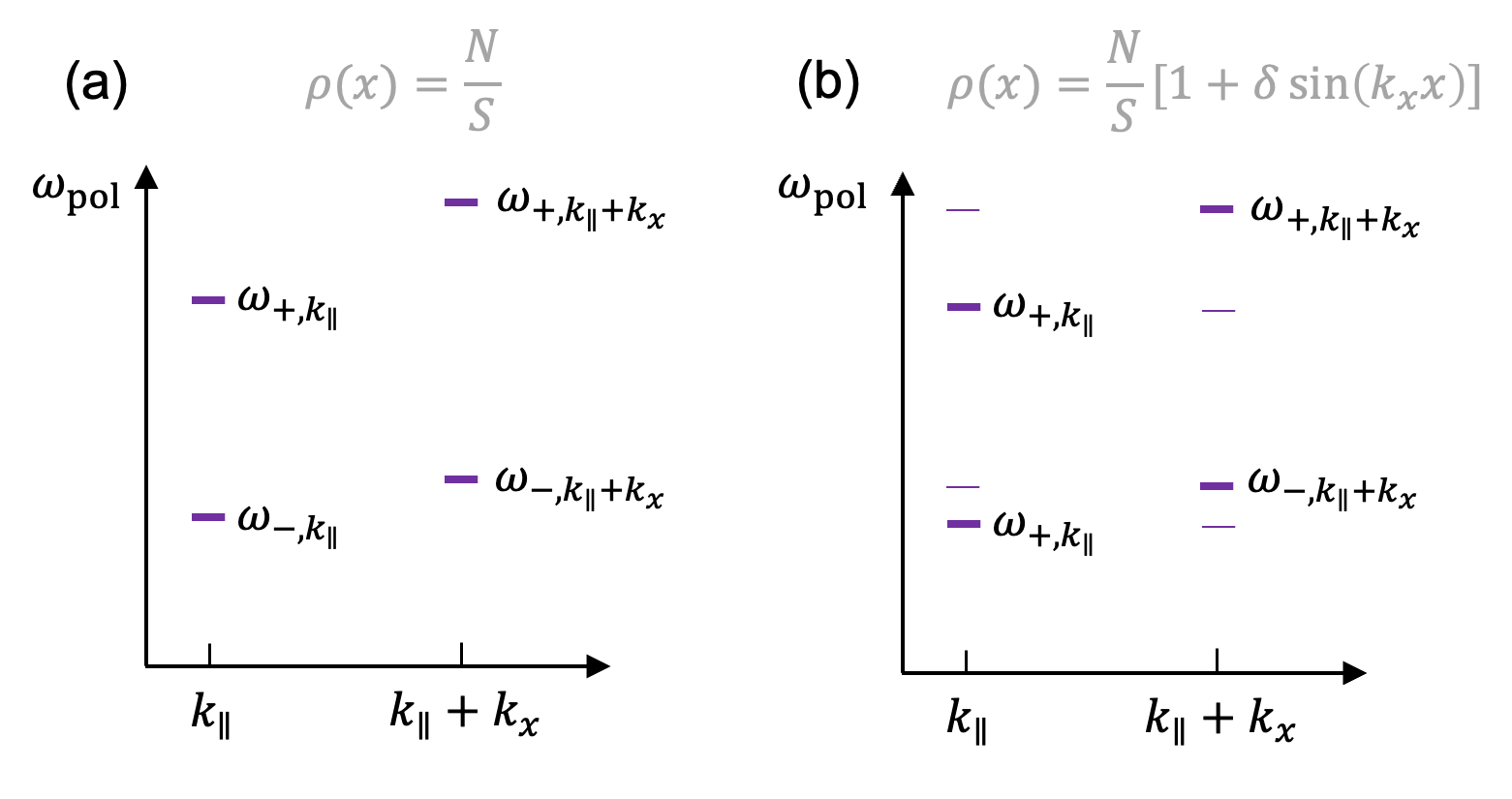
Figure 2: Illustration of the polariton dispersion relation in a planar Fabry–Pérot cavity for two different cases: (a) a homogeneous molecular density distribution along the 1D cavity mirror plane with $\rho(x)=\frac{N}{S}$; (b) an inhomogeneous molecular density distribution with $\rho(x)=\frac{N}{S}[1+\delta\sin(k_{x}x)]$ and $\delta\rightarrow 0$. For both cases, the polariton peaks at only two different in-plane wave vectors, $k_{\parallel}$ and $k_{\parallel}+k_{x}$, are explicitly plotted, where $k_{\parallel}$ is assumed to be near zero. For part (b), the polariton peaks at $k_{\parallel}$ and $k_{\parallel}+k_{x}$ mix with each other, leading to four side peaks at either $k_{\parallel}$ or $k_{\parallel}+k_{x}$.

The above derivations demonstrate that, given a sinusoidal density inhomogeneity in Eq. (19), four polariton peaks emerge at each in-plane wave vector $k_{\parallel}$. As illustrated in Fig. 2b, for small $k_{\parallel}$ values (left column), apart from the pair of polariton peaks corresponding to the homogeneous molecular distribution ($\omega_{\pm,k_{\parallel}}$), an additional pair of polariton peaks $\omega_{\pm,k_{\parallel}+k_{x}}$ appears in the spectra due to the interaction with the cavity mode at $k_{\parallel}+k_{x}$; similarly, for a large in-plane wave vector $k_{\parallel}+k_{x}$ (right column of Fig. 2b), apart from the pair of polariton peaks corresponding to the homogeneous molecular distribution ($\omega_{\pm,k_{\parallel}+k_{x}}$), an additional pair of polariton peaks $\omega_{\pm,k_{\parallel}}$ appears in the spectra due to the interaction with the cavity mode at $k_{\parallel}$. Below, at each $k_{\parallel}$ value, the pair of polariton peaks corresponding to the homogeneous molecular distribution will be called as the main polariton peaks; the additional pair of polariton peaks due to the interaction with the other cavity mode(s) will be called as the side polariton peaks.

At this point, we have understood that the spatial inhomogeneity of the molecules can cause the polariton states at different $k_{\parallel}$ values to mix with each other. Now, the remaining question is how to quantify the magnitude of this polariton mixing. As in experiments the intensity of the polariton signals is proportional to the photonic contribution in the polaritons, we now calculate the photonic weight of each polariton state mentioned above.

Because we have assumed that the density inhomogeneity is small ($\delta\rightarrow 0$), the photonic weights of the main polariton peaks should remain mostly the same as the homogeneous limit, i.e., they are the same as those in the JC model:

$$|\alpha_{k_{\parallel}}^{\pm,\rm main}|^{2} \approx\frac{(\omega_{0}-\omega_{\pm,k_{\parallel}})^{2}}{\Delta^{2}+(\omega_{0}-\omega_{\pm,k_{\parallel}})^{2}},$$ (26a)

$$|\alpha_{k_{\parallel}+k_{x}}^{\pm,\rm main}|^{2} \approx\frac{(\omega_{0}-\omega_{\pm,k_{\parallel}+k_{x}})^{2}}{\Delta^{2}+(\omega_{0}-\omega_{\pm,k_{\parallel}+k_{x}})^{2}}.$$ (26b)

For the side polaritons at small $$k_{\parallel}$$ values (the left column of Fig. 2b), the corresponding photonic weights can be obtained using Eq. (22b):

$$|\alpha_{k_{\parallel}+k_{x}}^{\pm,\rm side}|^{2} =\frac{1}{4}\delta^{2}|\alpha_{k_{\parallel}}^{\pm,\rm main}|^{2}\frac{\Delta^{4}}{(\omega_{\pm,k_{\parallel}}-\omega_{-,k_{\parallel}+k_{x}})^{2}(\omega_{\pm,k_{\parallel}}-\omega_{+,k_{\parallel}+k_{x}})^{2}}$$ (26c)

For the side polaritons at $$k_{\parallel}+k_{x}$$ (the right column of Fig. 2b), the corresponding photonic weights can be obtained using Eq. (22a):

$$|\alpha_{k_{\parallel}}^{\pm,\rm side}|^{2} =\frac{1}{4}\delta^{2}|\alpha_{k_{\parallel}+k_{x}}^{\pm,\rm main}|^{2}\frac{\Delta^{4}}{(\omega_{\pm,k_{\parallel}+k_{x}}-\omega_{-,k_{\parallel}})^{2}(\omega_{\pm,k_{\parallel}+k_{x}}-\omega_{+,k_{\parallel}})^{2}}$$ (26d)

The simple analytical forms of the polariton dispersion relation in Eqs. (25) and (26) quantify the impact of a weak sinusoidal density inhomogeneity on the polariton dispersion relation.

II.4.2 A general perturbative result

Given an arbitrary weak in-plane density inhomogeneity in 1D, it is possible to express the spatial density distribution as a linear combination of trigonometric functions:

$$\bar{\rho}(x)=\frac{S}{N}\rho(x)\approx 1+\sum_{l=1}^{M}\delta_{l}\sin(k_{l}x)+\delta^{\prime}_{l}\cos(k_{l}x).$$ (27)

where $\bar{\rho}(x)$ denotes the dimensionless molecular density distribution, $\delta_{l}$ and $\delta^{\prime}_{l}$ are small dimensionless variables, and $M$ is a finite number. Then, assuming that the cavity mode at $k_{\parallel}$ interacts with each of the other cavity modes $k_{\parallel}\pm k_{l}$ independently, we can directly use the above results to obtain the polariton dispersion relation corresponding to Eq. (27). At the in-plane wave vector $k_{\parallel}$, apart from the pair of main polariton peaks corresponding to the homogeneous limit, $4M$ side polariton peaks may emerge in the spectrum due to the interactions with $2M$ other cavity modes ($k_{\parallel}\pm k_{l}$ for $1\leq l\leq M$). The frequencies of these $4M$ side polariton peaks are the UP and the LP frequencies of the cavity modes at $k_{\parallel}\pm k_{l}$ in the homogeneous limit. At the in-plane wave vector $k_{\parallel}$, given a weak density inhomogeneity, the photonic weights of the main polariton peaks should be roughly the same as those in the homogeneous limit. For the photonic weights of the side polaritons, if we assume the side polariton peaks due to each of the other cavity modes are independent, according to Eq. (26), the photonic weights of the $4M$ side polariton peaks at $k_{\parallel}$ can be expressed as:

$$|\alpha_{k_{\parallel}+k_{l}}^{\pm,\rm side}|^{2} =\frac{1}{4}(|\delta_{l}|^{2}+|\delta^{\prime}_{l}|^{2})|\alpha_{k_{\parallel}}^{\pm,\rm main}|^{2}\frac{\Delta^{4}}{(\omega_{\pm,k_{\parallel}}-\omega_{-,k_{\parallel}+k_{l}})^{2}(\omega_{\pm,k_{\parallel}}-\omega_{+,k_{\parallel}+k_{l}})^{2}},$$ (28a)

$$|\alpha_{k_{\parallel}-k_{l}}^{\pm,\rm side}|^{2} =\frac{1}{4}(|\delta_{l}|^{2}+|\delta^{\prime}_{l}|^{2})|\alpha_{k_{\parallel}}^{\pm,\rm main}|^{2}\frac{\Delta^{4}}{(\omega_{\pm,k_{\parallel}}-\omega_{-,k_{\parallel}-k_{l}})^{2}(\omega_{\pm,k_{\parallel}}-\omega_{+,k_{\parallel}-k_{l}})^{2}}h(k_{\parallel}-k_{l}),$$ (28b)

where $h(k_{\parallel}-k_{l})$ denotes the Heaviside step function: $h(k_{\parallel}-k_{l})=1$ if $k_{\parallel}>k_{l}$ otherwise $h(k_{\parallel}-k_{l})=0$. In the above equations, the first term characterizes the photonic weights of the side polaritons due to the interaction with the main polariton peaks at $k_{\parallel}+k_{l}$; the second term characterizes the photonic weights of the side polaritons due to the interaction with the main polariton peaks at $k_{\parallel}-k_{l}$. Although our analysis for an arbitrary weak in-plane density inhomogeneity here is very primitive, this analysis shows that the complexity of the polariton dispersion relation directly correlates to the complexity of the in-plane density inhomogeneity in the $k$-space even when the inhomogeneity is weak.

If the in-plane density inhomogeneity is large, providing an analytical solution becomes very challenging. Instead, with numerical calculations, we can directly obtain the polariton dispersion relation for an arbitrary in-plane molecular density distribution. In the next section, we will provide numerical details on how to calculate polariton dispersion relations in a brute-force manner. A similar brute-force calculation was performed to study the effects of molecular disorders on the polariton dispersion relations in 1D cavities [13].

III Numerical details

To begin with, the cavity mirror plane was assumed to be 1D (along the $x$-axis). For an efficient description of the molecules, along the cavity mirror plane, periodic boundary conditions with a cell length of $L_{x}$ were applied. In each periodic cell, $N^{\rm grid}$ evenly distributed molecules (i.e., harmonic oscillators) along the $x$-axis (from $x=0$ to $L_{x}$) were used to represent the molecular distribution. The density inhomogeneity of molecules was represented by a distribution of different light-matter coupling strengths for each site: $g(x)=g_{0}\sqrt{\bar{\rho}(x)}$. A larger coupling strength at location $x$ indicates a larger molecular density distribution (or an increase in the thickness of the molecular layer) at the in-plane location $x$. Due to the use of periodic boundary conditions along the cavity mirror plane, the in-plane wave vector of each cavity mode became discrete: $k_{\parallel}=\frac{2\pi l}{L_{x}}$, where $l=1,2,\cdots,l_{x}^{\rm max}$ and $l_{x}^{\rm max}$ denotes the maximal number of the in-plane cavity modes included in the calculation. The corresponding cavity frequency for each cavity mode was represented as $\omega_{\rm c}(k_{\parallel})=\sqrt{\omega_{\perp}^{2}+\omega_{\parallel}^{2}}$, where $\omega_{\perp}$ denotes the fundamental cavity mode at zero in-plane angle and $\omega_{\parallel}\equiv ck_{\parallel}$.

Next, for the calculations of the 1D sinusoidal molecular density inhomogeneity, $\bar{\rho}(x)=1+\delta\sin(k_{x}x)$. The following set of parameters was taken to compare the analytical and the numerical results: $\delta=0.2$, $k_{x}=250$ cm^-1, $g_{0}=2.0$ cm^-1, $N^{\rm grid}=1080$, $l_{x}^{\rm max}=100$, $\omega_{\perp}=2320$ cm^-1, and $\Delta k_{\parallel}=\frac{2\pi}{L_{x}}=10$ cm^-1 (or $L_{x}=1$ mm). Then, the extended TC Hamiltonian was constructed in a similar form as Eq. (9), except that the uniform light-matter coupling strength $g_{0}$ was replaced by the site-dependent coupling strengths $g(x)$. With this set of parameters, the matrix form of the extended TC Hamiltonian had a dimension of $N_{\rm grid}+l_{x}^{\rm max}=1180$. The Python package numpy was used to diagonalize this matrix.

For the calculations of a 1D Gaussian molecular density distribution,

$$\bar{\rho}(x)=\mathcal{N}\exp\left[{-\frac{(x-L_{x}/2)^{2}}{2\sigma^{2}}}\right].$$ (29)

Here, $L_{x}=1$ mm denotes the length of the periodic cells along the cavity mirror plane; the Gaussian width $\sigma$ was chosen as different values; $\mathcal{N}$ denotes a normalization factor which enforces $\left\langle\bar{\rho}(x)\right\rangle\equiv\frac{1}{L_{x}}\int_{0}^{L_{x}}dx\bar{\rho}(x)=1$. In other words, along the cavity mirror plane (the $x$-direction), the molecular distribution was a series of periodic Gaussian peaks with a spacing of $L_{x}$. All the other parameters were kept the same as the case of the 1D sinusoidal molecular density inhomogeneity.

Finally, additional calculations were also performed when the cavity mirror plane was assumed to be 2D (along both the $x$- and the $y$-axis). Similar as the 1D cases, periodic boundary conditions were applied and the periodic cell had a size of $L_{x}\times L_{y}$. $N^{\rm grid}_{x}\times N^{\rm grid}_{y}$ molecules were evenly distributed in this 2D grid. The same as the 1D cases, the density inhomogeneity of molecules was represented by a distribution of different light-matter coupling strengths for each site: $g(x,y)=g_{0}\sqrt{\bar{\rho}(x,y)}$, where the dimensionless molecular density distribution $\bar{\rho}(x,y)=\frac{S}{N}\rho(x,y)$ will be given later in the manuscript. Along the $x$- or the $y$-axis, the in-plane wave vectors of the cavity modes were discretized: $k_{\parallel}^{x}=\frac{2\pi l}{L_{x}}$ and $k_{\parallel}^{y}=\frac{2\pi m}{L_{y}}$, where $l=1,2,\cdots,l_{x}^{\rm max}$ and $m=1,2,\cdots,m_{y}^{\rm max}$, respectively. The associated frequency for each cavity mode took the following form: $\omega_{\rm c}(\mathbf{k}_{\parallel})=\sqrt{\omega_{\perp}^{2}+(\omega_{\parallel}^{x})^{2}+(\omega_{\parallel}^{y})^{2}}$, where $\omega_{\parallel}^{x}=ck_{\parallel}^{x}$ and $\omega_{\parallel}^{y}=ck_{\parallel}^{y}$. The following set of parameters was used: $g_{0}=0.5$ cm^-1, $N^{\rm grid}_{x}=N^{\rm grid}_{y}=120$, $l_{x}^{\rm max}=m_{y}^{\rm max}=30$, $\omega_{\perp}=2320$ cm^-1, $\Delta k_{\parallel}^{x}=\frac{2\pi}{L_{x}}=30$ cm^-1 (or $L_{x}=0.33$ mm), and $\Delta k_{\parallel}^{y}=\frac{2\pi}{L_{y}}=30$ cm^-1 (or $L_{y}=0.33$ mm). With this set of parameters, the matrix form of the extended TC Hamiltonian took a dimension of $N_{\rm grid}^{x}\times N_{\rm grid}^{y}+l_{x}^{\rm max}\times l_{y}^{\rm max}=15300$. For such a fairly large matrix, instead of numpy, the Python package cupy was used for the matrix diagonalization with a NVIDIA RTX 3090 GPU.

IV Results

IV.1 1D inhomogeneity in the perturbative limit

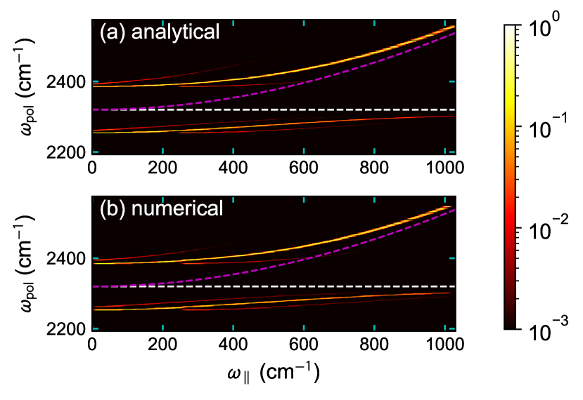
Figure 3: Polariton dispersion relation in an 1D Fabry–Pérot cavity with a sinusoidal molecular density inhomogeneity: $\bar{\rho}(x)=1+\delta\sin(k_{x}x)$ with $\delta=0.2$ and $k_{x}=250$ cm^-1. The analytical spectrum [part (a), Eqs. (25) and (26)] is plotted against the numerical result [part (b)] via directly diagonalizing the extended TC Hamiltonian. For both cases, the polariton intensity (on a logarithmic scale) is represented by the corresponding photonic weight of each eigenstate. The dashed white (magenta) line denote the bare molecular (photonic) excitation energy as a function of the in-plane frequency $\omega_{\parallel}=ck_{\parallel}$.

Given the sinusoidal density inhomogeneity defined in Eq. (19) [$\bar{\rho}(x)=1+\delta\sin(k_{x}x)$], Fig. 3a plots the polariton dispersion relation using the analytical solution in Eqs. (25) and (26) when the small parameter $\delta$ is chosen as $\delta=0.2$. In Fig. 3a, at each individual in-plane cavity frequency $\omega_{\parallel}$ ($=ck_{\parallel}$), apart from the pair of main polariton peaks, two side polariton peaks with weaker photonic weights appear in the spectrum. Overall, four additional side polariton branches (weak red lines) exist in the spectrum. Importantly, the side polariton branches at the left and the right sides are disconnected at $\omega_{\parallel}=250$ cm^-1. This is due to the interaction between the cavity modes at $k_{\parallel}$ and $k_{\parallel}+k_{x}$ values, as $k_{x}=250$ cm^-1 was chosen during the calculation.

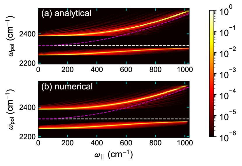
Figure 4: Polariton dispersion relation in an 1D Fabry–Pérot cavity with the molecular density inhomogeneity defined in Eq. (30). The analytical spectrum [part (a), Eqs. (28)] is plotted against the numerical result [part (b)] via directly diagonalizing the extended TC Hamiltonian.

To further examine our derivations, we perform numerical calculations of the polariton dispersion relation by directly diagonalizing the extended TC Hamiltonian. Fig. 3b plots the corresponding polariton spectrum from the numerical calculations. The agreement between Fig. 3a and Fig. 3b cross-validate both our analytical derivations and the numerical calculations.

Fig. 4 provides the comparison between the analytical and the numerical polariton dispersion relation for a more complicated weak 1D inhomogeneity:

$$\bar{\rho}(x)=1+\frac{\delta}{N_{\rm p}}\sum_{n=1}^{N_{\rm p}}\sin(k_{n}x).$$ (30)

Here, the small parameter $\delta=0.2$ is kept the same as that in Fig. 3, $k_{n}=10p_{n}$ cm^-1, and $p_{n}=2,3,5,\cdots,43$ denote $N_{\rm p}=13$ prime numbers. As a generalization of Fig. 3, both analytical results [using Eq. (28)] and numerical calculations demonstrate a comb of weak side polariton branches near the main upper and lower polariton branches. The consistency in Figs. 4a,b provides another cross-validation between the analytical and the numerical calculations.

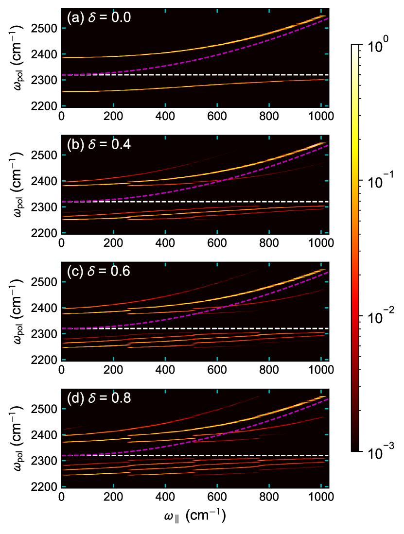
Figure 5: Numerically calculated polariton dispersion relation corresponding to the 1D sinusoidal molecular density inhomogeneity: $\bar{\rho}(x)=1+\delta\sin(k_{x}x)$. In each subplot, $k_{x}=250$ cm^-1 and the inhomogeneity amplitude is tuned as (a) $\delta=0.0$ (the homogeneous limit), (b) $\delta=0.4$, (c) $\delta=0.6$, and (d) $\delta=0.8$.

IV.2 1D sinusoidal inhomogeneity beyond the perturbative limit

Moving forward, using the sinusoidal molecular density inhomogeneity $\bar{\rho}(x)=1+\delta\sin(k_{x}x)$, we perform additional numerical calculations to investigate the modification of polariton dispersion relation beyond the perturbative limit. Fig. 5 plots the polariton spectra with different values of $\delta$, the amplitude of the sinusoidal density inhomogeneity. When $\delta=0$ (Fig. 5a, the homogeneous limit), we recover only two polariton branches, corresponding to the conventional polariton dispersion relation in the homogeneous limit. When $\delta=0.4$, 0.6, and 0.8 (Figs. 5b-d), apart from the two main polariton branches, more and more side polariton branches appear in the spectra. The number increase of side polariton branches indicate the higher order interactions between different cavity modes, which are completely discarded in our analytical derivations. Very importantly, in these spectra, different side polariton branches are still disconnected with a spacing of 250 cm^-1, indicating the interaction between cavity modes at $k_{\parallel}$ and $k_{\parallel}+k_{x}$ values, as $k_{x}=250$ cm^-1 was kept the same during the calculations. When $\delta=0.8$ (Fig. 5d), the main polariton branches are strongly altered by the other polariton branches. As a result, in this strong inhomogeneity limit, the definition of the main branches becomes obscure.

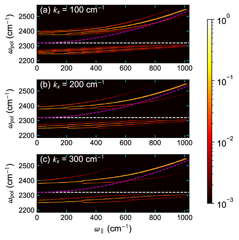
Figure 6: Numerically calculated polariton dispersion relation corresponding to the 1D sinusoidal molecular density inhomogeneity: $\bar{\rho}(x)=1+\delta\sin(k_{x}x)$. In each subplot, the inhomogeneity amplitude $\delta=0.5$ and $k_{x}$ is tuned to (a) 100 cm^-1, (b) 200 cm^-1, and (c) 300 cm^-1.

Fig. 6 plots a series of polariton spectra when $\delta=0.5$ is fixed and $k_{x}$ is tuned to (a) 100 cm^-1, (b) 200 cm^-1, and (c) 300 cm^-1, respectively. Because here $\delta$ is relatively large, multiple side polariton branches exist in each spectrum. However, in each spectrum, different side polariton branches are still disconnect with a spacing of the corresponding $k_{x}$ value.

IV.3 1D Gaussian distribution

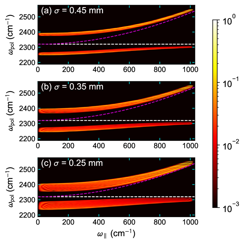
Figure 7: Numerically calculated polariton dispersion relation corresponding to the 1D Gaussian molecular in-plane density distribution defined in Eq. (29). In each subplot, the Gaussian width $\sigma$ is tuned as (a) $0.45$ mm, (b) $0.35$ mm, and (c) $0.25$ mm. Reducing the Gaussian width, i.e., increasing the molecular distribution inhomogeneity, enhances the broadening of the two main polariton branches.

Fig. 7 plots the polariton dispersion relation when the molecular distribution obeys the 1D Gaussian distribution defined in Eq. (29). When the width of the Gaussian distribution is $\sigma=0.45$ mm, the corresponding polariton dispersion relation (Fig. 7a) is very different from the cases of the sinusoidal inhomogeneity. Here, instead of the appearance of a few discrete side polariton branches, only the two main polariton branches remain. However, each polariton branch becomes significantly broadened. This polariton broadening can be understood as follows: as discussed around Eq. (28), because the Fourier transform of a spatial Gaussian distribution is still a Gaussian distribution in the frequency domain, the cavity mode at $k_{\parallel}$ can interact with all the cavity modes at the frequency neighbourhood $k_{\parallel}\pm\Delta k$, where $\Delta k\propto 1/\sigma$. As a result, instead of the emergence of a few side polariton branches, an enormous number of side polariton branches appear in the frequency neighbourhood of $k_{\parallel}$. Hence, the original two main polariton branches become effectively broadened. In Fig. 7b,c, when the Gaussian distribution has a smaller width ($\sigma=0.35$ mm or 0.25 mm), i.e., when the molecular distribution becomes more inhomogeneously, the polariton broadening becomes more significant. This trend agrees with our analysis above that the linewidth broadening at $k_{\parallel}$ is due to the interaction with the cavity modes at $k_{\parallel}\pm\Delta k$.

While it is known that the polariton linewidth broadening can be attributed to the homogeneous broadening of the molecular linewidth as well as the cavity loss [57, 4], the intriguing polariton broadening effect in Fig. 7 clearly shows that the large-scale, in-plane molecular density inhomogeneity can perhaps increase the polariton linewidth in a very significant manner. Such a linewidth broadening comes from the breakdown of the single-mode approximation and the emergence of the side polariton peaks due to the in-plane translational symmetry breaking. This finding provides another perspective to understand the origins of the polariton broadening observed in various experiments.

IV.4 2D distributions

The above calculations assumed that the cavity mirror plane was only 1D. This assumption might be questionable for planar Fabry–Pérot cavities with 2D cavity mirrors. To this end, we perform additional calculations to directly study the polariton dispersion relation when the cavity mirror plane becomes 2D.

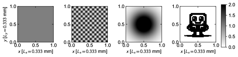
Figure 8: The four molecular density distributions $\bar{\rho}(x,y)$ considered in the 2D calculations: (a) the homogeneous limit when $\bar{\rho}(x,y)=1$; (b) the 2D sinusoidal inhomogeneity [Eq. (31)]; (c) the 2D Gaussian distribution [Eq. (32)]; (d) a cartoon pattern. For all the four cases, periodic boundary conditions are applied along the $xy$-plane, and the distributions on a single periodic cell are shown.

As shown in Fig. 8, four different 2D molecular distributions are considered. For the first homogeneous case (Fig. 8a), the corresponding polariton spectrum is plotted in Fig. 9a. Here, only two polariton branches are obtained, in agreement with the 1D case (Fig. 5a). Although the spectrum appears similarly as the 1D case, a significant difference is needed to be emphasized: in the 1D plot, the in-plane frequency $\omega_{\parallel}$ refers to $\omega_{\parallel}^{x}$, the cavity in-plane frequency along the cavity mirror plane direction (the $x$-direction); in the 2D plot, the in-plane frequency $\omega_{\parallel}$ refers to $\sqrt{|\omega_{\parallel}^{x}|^{2}+|\omega_{\parallel}^{y}|^{2}}$, an arbitrary combination of the in-plane frequencies in both the $x$- and the $y$-direction. In this homogeneous case, due to the preservation of the rotational symmetry along the 2D plane, $\omega_{\parallel}=\sqrt{|\omega_{\parallel}^{x}|^{2}+|\omega_{\parallel}^{y}|^{2}}$ is a good quantum number to characterize the cavity frequency dependence of the polariton spectrum.

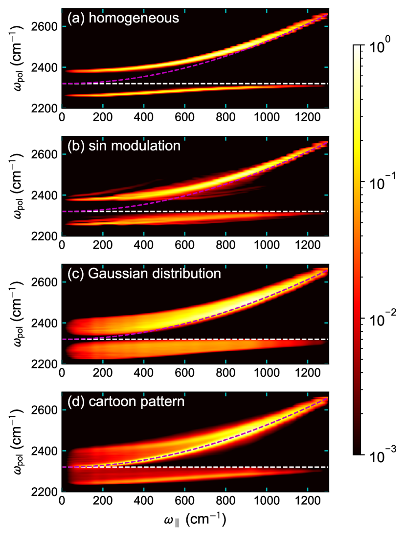
Figure 9: The polariton dispersion relations corresponding to the four 2D molecular distributions in Fig. 8, respectively.

Then, we consider a 2D sinusoidal molecular density inhomogeneity (Fig. 8b):

$$\bar{\rho}(x,y)=1+\delta\sin(k_{x}x)\sin(k_{y}y)$$ (31)

where $\delta=1.0$ and $k_{x}=k_{y}=250$ cm^-1.

Fig. 9b plots the polariton spectrum corresponding to the above 2D sinusoidal molecular density inhomogeneity. Here, apart from the two main polariton branches, a few side polariton branches can still be observed. Compared to the 1D cases, in an effort to efficiently simulate the 2D results, we have used a larger frequency spacing between adjacent cavity modes per dimension. As a result, the frequency resolution here is relatively low. Nevertheless, the observation of the a few side polariton branches suggests that the observations in the 1D sinusoidal distributions can be valid in the 2D as well.

Next, repeating the 1D calculations, we also consider a 2D Gaussian density distribution (Fig. 8c):

$$\bar{\rho}(x)=\mathcal{N}\exp\left[{-\frac{(x-\frac{L_{x}}{2})^{2}+(y-\frac{L_{y}}{2})^{2}}{2\sigma^{2}}}\right],$$ (32)

where $L_{x}=L_{y}=$ 0.333 mm, $\sigma=0.083$ mm, and $\mathcal{N}$ denotes a renormalization factor which enforces $\left\langle\bar{\rho}(x,y)\right\rangle\equiv\frac{1}{L_{x}L_{y}}\int_{0}^{L_{x}}dx\int_{0}^{L_{y}}dy\bar{\rho}(x,y)=1$. For this 2D Gaussian distribution, Fig. 9c plots the corresponding polariton dispersion relation. Here, two broadened polariton branches are observed, in agreement with the 1D correspondence (Fig. 7).

Finally, we perform an additional calculation when the molecular density distribution becomes Fig. 8d, a cartoon pattern. For such a density distribution, the corresponding polariton spectrum (Fig. 9d) demonstrates three major peaks: the two polariton branches as in Fig. 9a and a pure photonic excitation (the magenta line). The pure photonic excitation is related to the fact that there is some empty space in the 2D cartoon distribution, indicating that the photonic modes can sometimes be completely decoupled from the molecular excitations. Not surprisingly, due to a lack of symmetry in the molecular density distribution, the three major branches are also significantly blurred. One can understand such a peak blurring as the consequence of the mixture of the bright and dark states when the molecular in-plane density distribution becomes inhomogeneous: in this case, many dark modes contain a small photonic contribution. In the next section, we will discuss in more detail about the the mixture of the bright and dark states.

As a side note, because the molecular density distribution here does not preserve the in-plane rotational symmetry, the in-plane frequency $\omega_{\parallel}=\sqrt{|\omega_{\parallel}^{x}|^{2}+|\omega_{\parallel}^{y}|^{2}}$ may not be a good quantum number to describe the polariton spectrum. Instead, a better solution is perhaps to plot the polariton spectrum as a function of both $\omega_{\parallel}^{x}$ and $\omega_{\parallel}^{y}$, i.e., plotting a 3D polariton dispersion relation [21].

V Discussion

In an effort to better understand how the bright and the dark modes can mix with each other when the in-plane molecular density distribution becomes inhomogeneous, we further study the photonic weight distribution among the eigenstates in the VSC systems with broken in-plane translational symmetry.

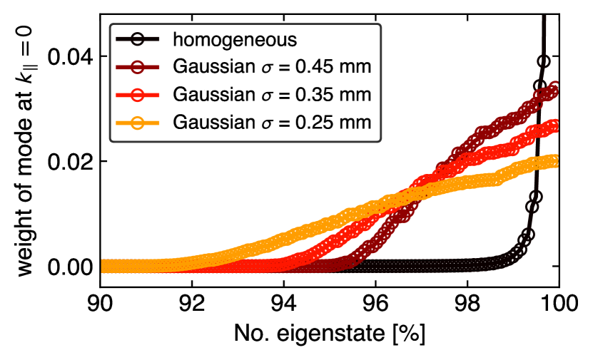
Figure 10: The $k_{\parallel}=0$ photonic weight distribution among all VSC eigenstates under a few different 1D conditions: the homogeneous limit (black) is compared against the three Gaussian distributions in Fig. 7: $\sigma=0.45$ mm (brown), $\sigma=$ 0.35 mm (red), and $\sigma=$ 0.25 mm (orange). The photon weights of different eigenstates are plotted in the ascend order. More eigenstates contain a non-zero $k_{\parallel}=0$ cavity photon contribution when the molecular in-plane distribution becomes more inhomogeneous.

Fig. 10 quantifies the weight distribution of the $k_{\parallel}=0$ cavity photon mode among the VSC eigenstates in a few different 1D systems. The homogeneous limit (black) is compared against the three Gaussian distributions discussed in Fig. 7: the distributions with Gaussian widths $\sigma=0.45$ mm (brown), $\sigma=0.35$ mm (red), and $\sigma=0.25$ mm (orange). For each case, the photon weights of different eigenstates are ranked in the ascend order. In the homogeneous limit, more than 99% of the eigenstates contain zero $k_{\parallel}=0$ photonic contribution, demonstrating a sharp separation between the bright (or polaritonic) and the dark modes. By contrast, when $\sigma=0.25$ mm, about 8% of the eigenstates contain a non-zero $k_{\parallel}=0$ photonic contribution. Clearly, with a reduced Gaussian width (or an increased density inhomogeneity), more eigenstates contain a non-zero contribution of the $k_{\parallel}=0$ cavity photon mode. This trend agrees with the increased polariton linewidths (i.e., more side polariton peaks) as observed in Fig. 7.

Previous experiments have indeed indicated the possibility of preparing the so-called gray states, i.e., a large amount of dark modes containing a non-zero photonic contribution, using materials with large energy disorder [61, 62]. However, our manuscript has demonstrated a very universal engineering technique, i.e., changing the molecular in-plane density distribution without altering the intrinsic properties of molecules, to achieve similar goals with the mechanism of in-plane translational symmetry breaking.

VI Conclusion

In summary, we have studied vibrational polaritons with structured in-plane molecular density distributions and the effects of in-plane translational symmetry breaking on the polariton dispersion relations. Due to the presence of the molecular density inhomogeneity (or the lack of in-plane translational symmetry), the single-mode approximation usually invoked in planar Fabry–Pérot microcavities becomes invalid, and the scattering between cavity modes at different in-plane wave vectors must be taken into account. As a result, even in the case of uniform molecular excitation frequencies plus simple planar Fabry–Pérot geometries (which have been assumed throughout this manuscript), complicated polariton dispersion relations could emerge by tuning the molecular density distribution along the cavity mirror plane.

In detail, for the case of a weak sinusoidal modulation of the homogeneous in-plane molecular density distribution, 1D perturbative calculations suggest that, in addition to the pair of main polariton branches, four additional side polariton branches could appear in the polariton dispersion relation. Numerical calculations further suggest the number increase of the side polariton branches when the sinusoidal inhomogeneity becomes stronger. More interestingly, for the case of a Gaussian molecular density distribution, numerical calculations show that the two main polariton branches can become significantly broadened. Such a polariton linewidth broadening is distinguished from other well-studied origins of polariton broadening: here the broadening results from the breakdown of the single-mode approximation and the scattering between cavity modes at different $\mathbf{k}_{\parallel}$ values, while our existing understanding of polariton broadening can be attributed mostly to either the homogeneous broadening of the molecular transition or the cavity loss.

While our derivations and calculations have used the parameters for VSC, the conclusions of this manuscript can also be applied to other types of collective strong couplings in planar Fabry–Pérot cavities such as exciton-polaritons. However, we believe that VSC might be a more advantageous platform for an experimental verification of our conclusions than electronic strong coupling, as the fabrication of in-plane molecular density inhomogeneity for VSC requires a spatial resolution of $0.01\sim 0.1$ mm (as shown in Fig. 8), which should be one-order-of-magnitude larger than that of electronic strong coupling due to the cavity frequency difference.

From a theoretical perspective, we have further emphasized the blurring between the bright and the dark modes with a Gaussian molecular in-plane density distribution. Whether such a state-blurring could impact polariton transport or even molecular dynamics in the dark is worthy of further investigation.

VII Acknowledgments

This work is supported by start-up funds from the University of Delaware Department of Physics and Astronomy.

VIII Data Availability Statement

The data that support the findings of this study will be available at Github upon publication of the manuscript.

References

• Weisbuch et al. [1992] C. Weisbuch, M. Nishioka, A. Ishikawa, and Y. Arakawa, “Observation of the coupled exciton-photon mode splitting in a semiconductor quantum microcavity,” Phys. Rev. Lett. 69, 3314–3317 (1992).
• Zhang et al. [2014] X. Zhang, C.-L. Zou, L. Jiang, and H. X. Tang, “Strongly coupled magnons and cavity microwave photons,” Phys. Rev. Lett. 113, 156401 (2014).
• Shalabney et al. [2015] A. Shalabney, J. George, J. Hutchison, G. Pupillo, C. Genet, and T. W. Ebbesen, “Coherent Coupling of Molecular Resonators with a Microcavity Mode,” Nat. Commun. 6, 5981 (2015).
• Long and Simpkins [2015] J. P. Long and B. S. Simpkins, “Coherent Coupling between a Molecular Vibration and Fabry–Perot Optical Cavity to Give Hybridized States in the Strong Coupling Limit,” ACS Photonics 2, 130–136 (2015).
• Wright, Nelson, and Weichman [2023] A. D. Wright, J. C. Nelson, and M. L. Weichman, “Rovibrational Polaritons in Gas-Phase Methane,” J. Am. Chem. Soc. 145, 5982–5987 (2023).
• Chikkaraddy et al. [2016] R. Chikkaraddy, B. de Nijs, F. Benz, S. J. Barrow, O. A. Scherman, E. Rosta, A. Demetriadou, P. Fox, O. Hess, and J. J. Baumberg, “Single-molecule strong coupling at room temperature in plasmonic nanocavities,” Nature 535, 127–130 (2016).
• Damari et al. [2019] R. Damari, O. Weinberg, D. Krotkov, N. Demina, K. Akulov, A. Golombek, T. Schwartz, and S. Fleischer, “Strong coupling of collective intermolecular vibrations in organic materials at terahertz frequencies,” Nat. Commun. 10, 3248 (2019).
• Canales et al. [2021] A. Canales, D. G. Baranov, T. J. Antosiewicz, and T. Shegai, “Abundance of cavity-free polaritonic states in resonant materials and nanostructures,” J. Chem. Phys. 154, 024701 (2021)arXiv:2010.07727 .
• Yoo et al. [2021] D. Yoo, F. de León-Pérez, M. Pelton, I.-H. Lee, D. A. Mohr, M. B. Raschke, J. D. Caldwell, L. Martín-Moreno, and S.-H. Oh, “Ultrastrong plasmon–phonon coupling via epsilon-near-zero nanocavities,” Nat. Photonics 15, 125–130 (2021)arXiv:2003.00136 .
• Deng, Haug, and Yamamoto [2010] H. Deng, H. Haug, and Y. Yamamoto, “Exciton-Polariton Bose–Einstein Condensation,” Rev. Mod. Phys. 82, 1489–1537 (2010).
• Carusotto and Ciuti [2013] I. Carusotto and C. Ciuti, “Quantum fluids of light,” Rev. Mod.Phys. 85, 299–366 (2013)arXiv:2211.10980 .
• Agranovich, Litinskaia, and Lidzey [2003] V. M. Agranovich, M. Litinskaia, and D. G. Lidzey, “Cavity polaritons in microcavities containing disordered organic semiconductors,” Phys. Rev. B 67, 085311 (2003).
• Michetti and La Rocca [2005] P. Michetti and G. C. La Rocca, “Polariton states in disordered organic microcavities,” Phys. Rev. B 71, 115320 (2005).
• Tanese et al. [2013] D. Tanese, H. Flayac, D. Solnyshkov, A. Amo, A. Lemaître, E. Galopin, R. Braive, P. Senellart, I. Sagnes, G. Malpuech, and J. Bloch, “Polariton condensation in solitonic gap states in a one-dimensional periodic potential,” Nat. Commun. 4, 1749 (2013).
• Schneider et al. [2017] C. Schneider, K. Winkler, M. D. Fraser, M. Kamp, Y. Yamamoto, E. A. Ostrovskaya, and S. Höfling, “Exciton-polariton trapping and potential landscape engineering,” Rep. Prog. Phys. 80, 016503 (2017)arXiv:1510.07540 .
• Mandal et al. [2023a] A. Mandal, D. Xu, A. Mahajan, J. Lee, M. Delor, and D. R. Reichman, “Microscopic Theory of Multimode Polariton Dispersion in Multilayered Materials,” Nano Lett. 23, 4082–4089 (2023a).
• Ohadi et al. [2012] H. Ohadi, E. Kammann, T. C. H. Liew, K. G. Lagoudakis, A. V. Kavokin, and P. G. Lagoudakis, “Spontaneous Symmetry Breaking in a Polariton and Photon Laser,” Phys. Rev. Lett. 109, 016404 (2012)arXiv:1204.5969 .
• Cao and Yan [2019] Y. Cao and P. Yan, “Exceptional magnetic sensitivity of PT-symmetric cavity magnon polaritons,” Phys. Rev. B 99, 214415 (2019)arXiv:1901.10685 .
• Chestnov et al. [2023] I. Chestnov, K. Kondratenko, S. Demirchyan, and A. Kavokin, “Symmetry breaking and superfluid currents in a split-ring spinor polariton condensate,” Phys. Rev. B 107, 245302 (2023).
• Vasista et al. [2022] A. B. Vasista, E. J. C. Dias, F. J. García de Abajo, and W. L. Barnes, “Role of Symmetry Breaking in Observing Strong Molecule–Cavity Coupling Using Dielectric Microspheres,” Nano Lett. 22, 6737–6743 (2022).
• Łempicka Mirek et al. [2022] K. Łempicka Mirek, M. Król, H. Sigurdsson, A. Wincukiewicz, P. Morawiak, R. Mazur, M. Muszyński, W. Piecek, P. Kula, T. Stefaniuk, M. Kamińska, L. D. Marco, P. G. Lagoudakis, D. Ballarini, D. Sanvitto, J. Szczytko, and B. Piętka, “Electrically tunable berry curvature and strong light-matter coupling in liquid crystal microcavities with 2d perovskite,” Sci. Adv. 8, eabq7533 (2022).
• Thomas et al. [2016] A. Thomas, J. George, A. Shalabney, M. Dryzhakov, S. J. Varma, J. Moran, T. Chervy, X. Zhong, E. Devaux, C. Genet, J. A. Hutchison, and T. W. Ebbesen, “Ground-State Chemical Reactivity under Vibrational Coupling to the Vacuum Electromagnetic Field,” Angew. Chemie Int. Ed. 55, 11462–11466 (2016).
• Ahn et al. [2023] W. Ahn, J. F. Triana, F. Recabal, F. Herrera, and B. S. Simpkins, “Modification of ground-state chemical reactivity via light–matter coherence in infrared cavities,” Science 380, 1165–1168 (2023).
• Thomas et al. [2019] A. Thomas, L. Lethuillier-Karl, K. Nagarajan, R. M. A. Vergauwe, J. George, T. Chervy, A. Shalabney, E. Devaux, C. Genet, J. Moran, and T. W. Ebbesen, “Tilting a Ground-State Reactivity Landscape by Vibrational Strong Coupling,” Science 363, 615–619 (2019).
• Hirai et al. [2021] K. Hirai, H. Ishikawa, T. Chervy, J. A. Hutchison, and H. Uji-i, “Selective Crystallization via Vibrational Strong Coupling,” Chem. Sci. 12, 11986–11994 (2021).
• Imperatore, Asbury, and Giebink [2021] M. V. Imperatore, J. B. Asbury, and N. C. Giebink, “Reproducibility of Cavity-Enhanced Chemical Reaction Rates in the Vibrational Strong Coupling Regime,” J. Chem. Phys. 154, 191103 (2021).
• Wiesehan and Xiong [2021] G. D. Wiesehan and W. Xiong, “Negligible Rate Enhancement from Reported Cooperative Vibrational Strong Coupling Catalysis,” J. Chem. Phys. 155, 241103 (2021).
• Fidler et al. [2023] A. P. Fidler, L. Chen, A. M. McKillop, and M. L. Weichman, “Ultrafast dynamics of CN radical reactions with chloroform solvent under vibrational strong coupling,” arXiv  (2023)arXiv:2307.04875 .
• Dunkelberger et al. [2016] A. D. Dunkelberger, B. T. Spann, K. P. Fears, B. S. Simpkins, and J. C. Owrutsky, “Modified relaxation dynamics and coherent energy exchange in coupled vibration-cavity polaritons,” Nat. Commun. 7, 1–10 (2016).
• Xiang et al. [2020] B. Xiang, R. F. Ribeiro, M. Du, L. Chen, Z. Yang, J. Wang, J. Yuen-Zhou, and W. Xiong, “Intermolecular Vibrational Energy Transfer Enabled by Microcavity Strong Light–Matter Coupling,” Science 368, 665–667 (2020).
• Chen et al. [2022] T.-T. Chen, M. Du, Z. Yang, J. Yuen-Zhou, and W. Xiong, “Cavity-enabled Enhancement of Ultrafast Intramolecular Vibrational Redistribution over Pseudorotation,” Science 378, 790–794 (2022).
• Simpkins, Dunkelberger, and Vurgaftman [2023] B. S. Simpkins, A. D. Dunkelberger, and I. Vurgaftman, “Control, Modulation, and Analytical Descriptions of Vibrational Strong Coupling,” Chem. Rev. 123, 5020–5048 (2023).
• Galego et al. [2019] J. Galego, C. Climent, F. J. Garcia-Vidal, and J. Feist, “Cavity Casimir-Polder Forces and Their Effects in Ground-State Chemical Reactivity,” Phys. Rev. X 9, 021057 (2019).
• Campos-Gonzalez-Angulo, Ribeiro, and Yuen-Zhou [2019] J. A. Campos-Gonzalez-Angulo, R. F. Ribeiro, and J. Yuen-Zhou, “Resonant Catalysis of Thermally Activated Chemical Reactions with Vibrational Polaritons,” Nat. Commun. 10, 4685 (2019).
• Hoffmann et al. [2020] N. M. Hoffmann, L. Lacombe, A. Rubio, and N. T. Maitra, “Effect of Many Modes on Self-Polarization and Photochemical Suppression in Cavities,” J. Chem. Phys. 153, 104103 (2020).
• Li, Mandal, and Huo [2021] X. Li, A. Mandal, and P. Huo, “Cavity Frequency-Dependent Theory for Vibrational Polariton Chemistry,” Nat. Commun. 12, 1315 (2021).
• Fischer and Saalfrank [2021] E. W. Fischer and P. Saalfrank, “Ground State Properties and Infrared Spectra of Anharmonic Vibrational Polaritons of Small Molecules in Cavities,” J. Chem. Phys. 154, 104311 (2021).
• Yang and Cao [2021] P. Y. Yang and J. Cao, “Quantum Effects in Chemical Reactions under Polaritonic Vibrational Strong Coupling,” J. Phys. Chem. Lett. 12, 9531–9538 (2021).
• Wang et al. [2022] D. S. Wang, T. Neuman, S. F. Yelin, and J. Flick, “Cavity-Modified Unimolecular Dissociation Reactions via Intramolecular Vibrational Energy Redistribution,” J. Phys. Chem. Lett 13, 3317–3324 (2022).
• Flick et al. [2017] J. Flick, M. Ruggenthaler, H. Appel, and A. Rubio, “Atoms and Molecules in Cavities, from Weak to Strong Coupling in Quantum-Electrodynamics (QED) Chemistry,” Proc. Natl. Acad. Sci. 114, 3026–3034 (2017).
• Riso et al. [2022] R. R. Riso, T. S. Haugland, E. Ronca, and H. Koch, “Molecular Orbital Theory in Cavity QED Environments,” Nat. Commun. 13, 1368 (2022).
• Schäfer et al. [2022] C. Schäfer, J. Flick, E. Ronca, P. Narang, and A. Rubio, “Shining Light on the Microscopic Resonant Mechanism Responsible for Cavity-Mediated Chemical Reactivity,” Nat. Commun. 13, 7817 (2022).
• Bonini and Flick [2021] J. Bonini and J. Flick, “Ab Initio Linear-Response Approach to Vibro-polaritons in the Cavity Born-Oppenheimer Approximation,” J. Chem. Theory Comput. 18, 2764–2773 (2021).
• Yang et al. [2021] J. Yang, Q. Ou, Z. Pei, H. Wang, B. Weng, Z. Shuai, K. Mullen, and Y. Shao, “Quantum-Electrodynamical Time-Dependent Density Functional Theory within Gaussian Atomic Basis,” J. Chem. Phys. 155, 064107 (2021).
• Rosenzweig et al. [2022] B. Rosenzweig, N. M. Hoffmann, L. Lacombe, and N. T. Maitra, “Analysis of the Classical Trajectory Treatment of Photon Dynamics for Polaritonic Phenomena,” J. Chem. Phys. 156, 054101 (2022)arXiv:2111.11957 .
• Triana, Hernández, and Herrera [2020] J. F. Triana, F. J. Hernández, and F. Herrera, “The Shape of the Electric Dipole Function Determines the Sub-picosecond Dynamics of Anharmonic Vibrational Polaritons,” J. Chem. Phys. 152, 234111 (2020).
• Li, Subotnik, and Nitzan [2020] T. E. Li, J. E. Subotnik, and A. Nitzan, “Cavity Molecular Dynamics Simulations of Liquid Water under Vibrational Ultrastrong Coupling,” Proc. Natl. Acad. Sci. 117, 18324–18331 (2020).
• Campos-Gonzalez-Angulo et al. [2023] J. A. Campos-Gonzalez-Angulo, Y. R. Poh, M. Du, and J. Yuen-Zhou, “Swinging between shine and shadow: Theoretical advances on thermally activated vibropolaritonic chemistry,” J. Chem. Phys. 158, 230901 (2023).
• Suyabatmaz and Ribeiro [2023] E. Suyabatmaz and R. F. Ribeiro, “Vibrational Polariton Transport in Disordered Media,” J. Chem. Phys. 159 (2023), 10.1063/5.0156008/2902632.
• Ribeiro et al. [2018] R. F. Ribeiro, L. A. Martínez-Martínez, M. Du, J. Campos-Gonzalez-Angulo, and J. Yuen-Zhou, “Polariton Chemistry: Controlling Molecular Dynamics with Optical Cavities,” Chem. Sci. 9, 6325–6339 (2018).
• Li et al. [2022] T. E. Li, B. Cui, J. E. Subotnik, and A. Nitzan, “Molecular Polaritonics: Chemical Dynamics Under Strong Light–Matter Coupling,” Annu. Rev. Phys. Chem. 73, 43–71 (2022).
• Fregoni, Garcia-Vidal, and Feist [2022] J. Fregoni, F. J. Garcia-Vidal, and J. Feist, “Theoretical Challenges in Polaritonic Chemistry,” ACS Photonics 9, 1096–1107 (2022).
• Mandal et al. [2023b] A. Mandal, M. A. Taylor, B. M. Weight, E. R. Koessler, X. Li, and P. Huo, “Theoretical Advances in Polariton Chemistry and Molecular Cavity Quantum Electrodynamics,” Chem. Rev. 123, 9786–9879 (2023b).
• Ruggenthaler, Sidler, and Rubio [2023] M. Ruggenthaler, D. Sidler, and A. Rubio, “Understanding Polaritonic Chemistry from Ab Initio Quantum Electrodynamics,” Chem. Rev. 123, 11191–11229 (2023)arXiv:2211.04241 .
• Xiang et al. [2021] B. Xiang, J. Wang, Z. Yang, and W. Xiong, “Nonlinear infrared polaritonic interaction between cavities mediated by molecular vibrations at ultrafast time scale,” Sci. Adv. 7, eabf6397 (2021).
• Li [2024] T. E. Li, “Mesoscale Molecular Simulations of Fabry–Pérot Vibrational Strong Coupling,” submitted  (2024).
• Houdré, Stanley, and Ilegems [1996] R. Houdré, R. P. Stanley, and M. Ilegems, “Vacuum-field Rabi Splitting in the Presence of Inhomogeneous Broadening: Resolution of a Homogeneous Linewidth in an Inhomogeneously Broadened System,” Phys. Rev. A 53, 2711–2715 (1996).
• Jaynes and Cummings [1963] E. Jaynes and F. Cummings, “Comparison of Quantum and Semiclassical Radiation Theories with Application to the Beam Maser,” Proc. IEEE 51, 89–109 (1963).
• Tavis and Cummings [1968] M. Tavis and F. W. Cummings, “Exact Solution for an N-Molecule—Radiation-Field Hamiltonian,” Phys. Rev. 170, 379–384 (1968).
• Tavis and Cummings [1969] M. Tavis and F. W. Cummings, “Approximate Solutions for an N-Molecule-Radiation-Field Hamiltonian,” Phys. Rev. 188, 692–695 (1969).
• Son et al. [2022] M. Son, Z. T. Armstrong, R. T. Allen, A. Dhavamani, M. S. Arnold, and M. T. Zanni, “Energy cascades in donor-acceptor exciton-polaritons observed by ultrafast two-dimensional white-light spectroscopy,” Nat. Commun. 13, 7305 (2022).
• George et al. [2024] A. George, T. Geraghty, Z. Kelsey, S. Mukherjee, G. Davidova, W. Kim, and A. J. Musser, “Controlling the Manifold of Polariton States Through Molecular Disorder,” Adv. Opt. Mater. , 2302387 (2024)arXiv:2309.13178 .