Offline Imitation of Badminton Player Behavior via Experiential Contexts and Brownian Motion

Abstract

In the dynamic and rapid tactic involvements of turn-based sports, badminton stands out as an intrinsic paradigm that requires alter-dependent decision-making of players. While the advancement of learning from offline expert data in sequential decision-making has been witnessed in various domains (e.g., video games), how to rally-wise imitate the behaviors of human players from offline badminton matches has remained underexplored. Replicating opponents’ behavior benefits players by allowing them to undergo strategic development with direction before matches. However, directly applying existing methods suffers from the inherent hierarchy of the match and the compounding effect due to the turn-based nature of players alternatively taking actions. In this paper, we propose RallyNet, a novel hierarchical offline imitation learning model for badminton player behaviors: (i) RallyNet captures players’ decision dependencies by modeling decision-making processes as a contextual Markov decision process. (ii) To facilitate the decision-making of an agent, RallyNet leverages the experience to generate context as the agent’s intent in the rally. (iii) To generate more realistic behavior, RallyNet leverages Geometric Brownian Motion (GBM) to model the interactions between players by introducing a valuable inductive bias for learning player behaviors. In this manner, RallyNet links player intents with interaction models with GBM, providing an understanding of real interactions for sports analytics. We extensively validate RallyNet with the largest available real-world badminton dataset consisting of men’s and women’s singles, demonstrating its ability to adeptly imitate player behaviors. The results illustrate RallyNet’s superiority, surpassing offline imitation learning methods and state-of-the-art turn-based approaches by at least 16% in the mean of rule-based agent normalization score. In addition, several practical use cases are discussed to showcase the applicability of RallyNet.

I Introduction

Collecting historical data and simulating agents’ behaviors have been widely explored to study and replicate specific scenarios in various domains, e.g., autonomous driving [2], robots [3, 4] and gaming [5]. In sports analytics, one of the major goals is to understand and investigate the tactics of teams and individuals. Given the rapid development of information technology, massive amounts of fine-grained behavioral records in various sports domains have been collected to train models for analysis [6, 7, 8, 9]. On the other hand, these behavioral records also help models reproduce strategic behavior. The applicability to the replication of player strategic behavior could assist coaches in devising winning strategies. Moreover, it opens avenues for numerous applications, including tactics simulation [6] and sports broadcasting [10]. However, applying this learning to an online environment, particularly for badminton, a turn-based sport, poses unique challenges. Unlike basketball and football, where players dictate their own positions, in badminton, a player’s state (e.g., receiving position) is determined by the opponent. As a result, conventional imitation learning methods employed in basketball [11] and football [6] cannot be directly applied to turn-based sports since finding authentic opponents for the agent to interact with and enhance its strategies in a realistic game scenario is impractical.

Therefore, we focus on leveraging offline behavioral records to replicate turn-based player behavior, employing offline imitation learning (IL) since it provides insights from past match data, enabling coaches and players to infer winning strategies. To effectively apply offline IL in badminton, we define three goals as key criteria to assess the model’s suitability for badminton scenarios.

• Behavioral Sequence Similarity: The learned agent’s behavior sequences should closely mirror real-world rally content, capturing the order of shot types, shuttlecock trajectories, and player movement patterns.

• Rally Duration Realism: To accurately depict how actual players participate in matches, it is crucial for the learned agents to reproduce the genuine duration of rallies.

• Outcome Consistency: Interactions between learned agents should yield consistent results with actual rallies, ensuring that simulated rallies reflect the competitive dynamics of actual gameplay.

Numerous past investigations have demonstrated success in offline IL, with Behavior Cloning (BC) standing out as a classical IL method for replicating a player’s actions. The effectiveness of offline IL has recently been illustrated, including hierarchical imitation learning (HIL) models [12, 13]. HIL models can excel in capturing the intrinsic hierarchy present in turn-based sports. For instance, in badminton, players often decide on a tactic before determining each action in a rally based on that strategy. Although hierarchical BC-based approaches enrich imitated expressivity in the long-horizontal task, none of them were designed for turn-based sports, which consist of multiple players taking actions alternatively to form a rally.

Therefore, there are two challenges to applying existing HIL methods directly for turn-based sports: 1) Leveraging experience. When players encounter situations that have appeared in their experience (e.g., from training and previous matches), they usually take corresponding actions for returning shots. Furthermore, in the same situation, there may be a wide variety of different corresponding behaviors in their experience. It is challenging to leverage experience to provide the helpful information of the action for the agent. 2) Alternative decision-making. In a turn-based sport, the state of each player is determined by the actions of not only themselves but also other players. Thus, the errors of an agent’s decision impact the decisions of other agents, resulting in more serious compounding errors. This challenge transcends the domain of multiple policies. It underscores how a player’s decision not only engages multiple policies but also directly determines the opponent’s state, shaping their decision dynamics. This stands in contrast to other multi-agent games such as board games, card games, and non-turn-based sports like basketball. In these games, a player’s actions do not directly dictate the opponent’s state since the actions decided by a player are not equivalent to the opponent’s state. This underscores the unique characteristic of turn-based sports.

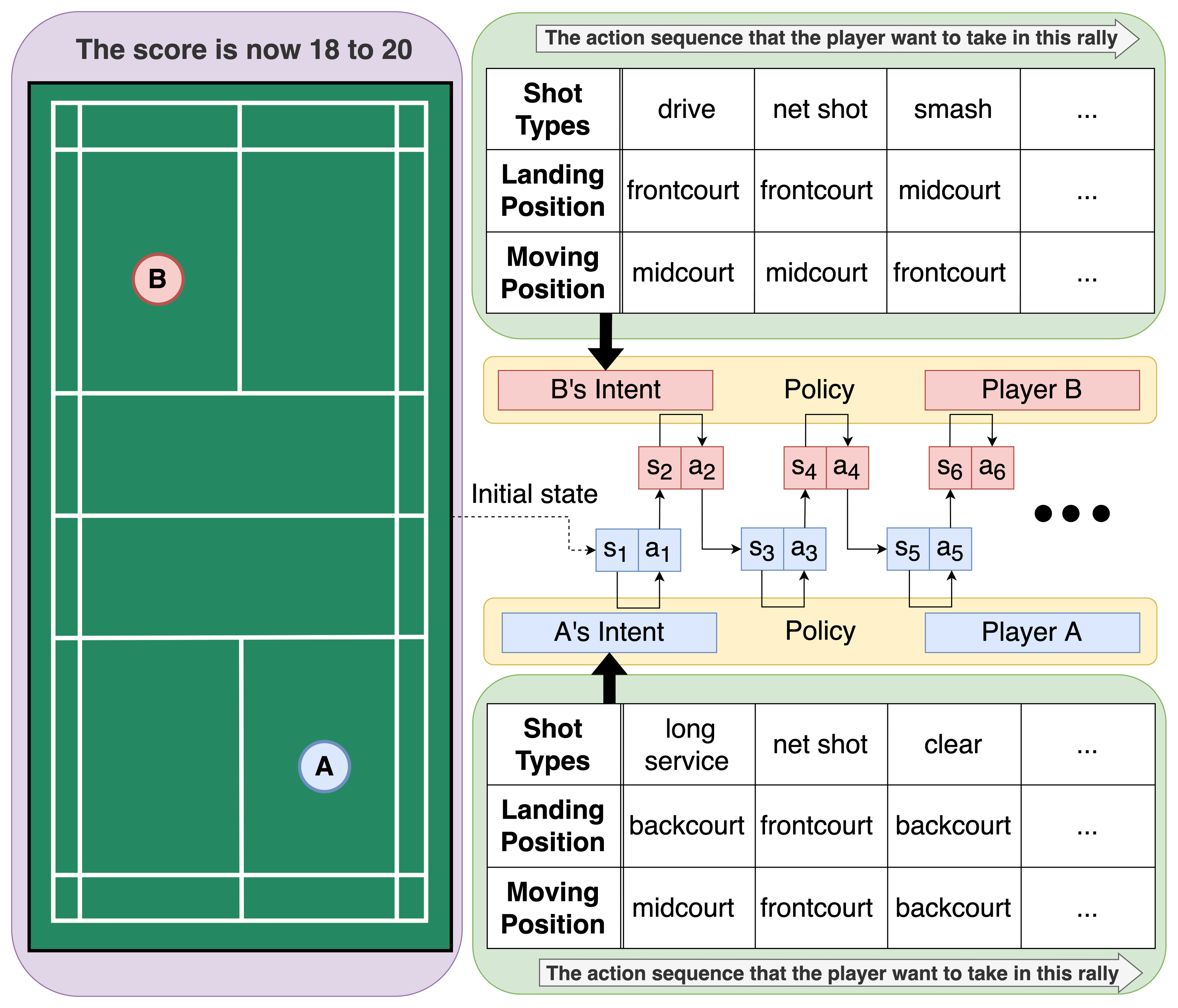
Figure 1: An illustration of RallyNet in a badminton rally.

To address these challenges, we propose a hierarchical offline imitation learning model via experiential context and geometric Brownian motion (RallyNet) to capture long-term decision dependencies by modeling decision-making processes in turn-based sports as contextual Markov decision processes (CMDP) [14]. Based on the CMDP setting, the Experiential Context Selector (ECS) was designed by establishing the context space from experiences and selecting a context in the space as the agent’s intent to mimic the decision-making of the agents following their intents in the rally. This enables the agent’s behavior throughout the rally to not be influenced by partially incorrect decisions from the agent. If an incorrect decision occurs, adhering to the intent prevents it from spreading, enhancing decision reliability and providing the physical explanations of the context to understand the intent behind the agent’s decisions.

As the interactions between players are similar to those between particles, we introduce Latent Geometric Brownian Motion (LGBM) to capture the interactions between players. LGBM leverages the intrinsic capacity of Geometric Brownian Motion (GBM), characterized as a continuous-time stochastic process with Gaussian distributed increments [15], to model randomness and heavy-tailed distributions inherent in turn-based sports interactions. Players participating in a rally alternately complete GBM in latent space to enable the agent’s decision-making to jointly consider the opponent’s behavior. In this manner, RallyNet is able to generate more realistic behavior in alternative decision-making. Figure 1 illustrates how RallyNet is applied to a turn-based sport, and uses a badminton singles match as an example. An initial state of the rally including two players’ positions and score information is provided to recover the content of the rally.

We highlight our main contributions as follows:

• We propose a novel HIL model via experiential context and geometric Brownian motion named RallyNet to learn player decision-making strategies in turn-based sports. To the best of our knowledge, this is the first work that imitates turn-based player behaviors.

• RallyNet models turn-based decision-making processes as CMDP, and leverages experiences to generate agents’ intent, reducing the impact of partial incorrect decisions from the agent on overall behavior and enabling explanations to understand the intent behind the player’s behavior. In addition, we introduce the latent geometric Brownian motion to capture the interactions between players, making the generated behavior more realistic.

• We quantitatively validate the performance of RallyNet in a real-world badminton dataset with men’s singles and women’s singles, which demonstrates that RallyNet attains superior performance than prior offline IL methods and the state-of-the-art turn-based supervised method. surpassing them by 16% in the mean of the rule-based agent normalized score.

II Preliminaries

II-A Badminton: A Typical Example of a Turn-Based Sport

For simplicity, we consider a badminton game with two players (i.e., singles matches) as the demonstration example. The badminton environment has a real-world badminton court, which includes one player on each side, a shuttlecock, the net, and the boundary. As shown in Figure 1, the state of the player who hits the shuttlecock consists of the score information, the 2-dimensional position of the shuttlecock, the shot type to receive, the player’s position, the opponent’s position, and the moving vector of the opponent (e.g., move forward 1m). The action of the player consists of the landing position of the shuttlecock, the shot type (the shuttlecock type to hit), and the moving position to go to after returning the shuttlecock.

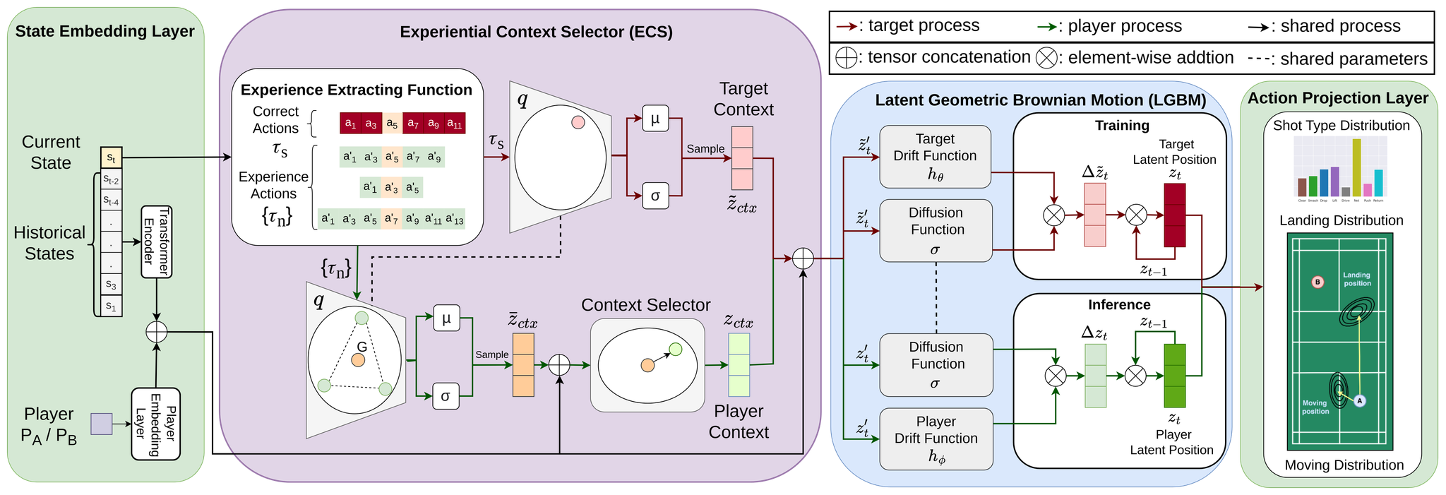
Figure 2: The framework of RallyNet.

II-B The Contextual Markov Decision Process

A Markov Decision Process (MDP) [16] is defined by a tuple $(S,A,T(y|x,a),R(x),\gamma)$, where $S$ is a set of states, $A$ is a set of possible actions agents can take, $T(y|x,a)$ is the transition probability, $R(x)$ is a reward function, and $\gamma\in[0,1)$ is the discount factor. At the $t$-th time step, the agent receives a state $s_{t}\in S$, then takes an action $a_{t}\in A$ according to a policy $\pi(a_{t}|s_{t})$. It is noted that the reward signal and the interaction with the environment are not available in the offline setting in this paper. The Contextual Markov Decision Process (CMDP) [14] leverages side information to extend the standard MDP with multiple contexts. A CMDP is defined by a tuple $(C,S,A,M)$, where $C$ is a set of contexts and $M$ is a function which maps a context $c\in C$ to MDP parameters $M(c)=\{R^{c},T^{c}\}$.

II-C Problem Formulation

For the badminton game with two players, we denote $P_{A}$ as the starting player and $P_{B}$ as the other player for each rally. Let $\mathcal{R}=\{T_{r}\}^{|\mathcal{R}|}_{r=1}$ denote historical rallies of badminton matches, where the rally is composed of a sequence of state-action pairs. The $r$-th rally is denoted as $T_{r}=\{(s_{1}^{P_{A}},a_{1}^{P_{A}}),(s_{1}^{P_{B}},a_{1}^{P_{B}}),…,(s_{|T_{r}|}^{p},a_{|T_{r}|}^{p})\}$. At the $t$-th step, $s_{t}^{p}$ and $a_{t}^{p}$ represent the state and action of the player who takes action, respectively, where $p\in\{P_{A},P_{B}\}$ represents that the step is related to either $P_{A}$ or $P_{B}$. $p=P_{A}$ when $t=2i-1$ and $p=P_{B}$ when $t=2i$, where $i=1,2,\dots,|T_{r}|$. The action consists of the landing positions, shot type, and moving positions represented by $a_{t}^{p}=\langle l_{t}^{p},t_{t}^{p},m_{t}^{p}\rangle$. The imitation learning task for turn-based sports is to learn a policy that can recover players’ demonstrations from a set of historical rallies $\mathcal{R}$. Formally, for each demonstration rally in $\mathcal{R}$, given initial state $s_{1}^{a}$ of the $r$-th rally $T_{r}$, our goal is to recover the rally $T_{r}$.

We formulate the decision-making process in badminton games as CMDP: The context space $C$ consists of contexts with the dimension $K$. At the beginning of each rally, the agent chooses a context $c\in C$, where $c$ represents the agent’s desired intent for the rally. Subsequently, the chosen MDP corresponding to context $c$ is applied throughout the rally until termination. A rally would terminate when any of the following termination conditions are satisfied: (i) The agent misses the shot; (ii) The shuttlecock does not come over the net; (iii) The shuttlecock falls out of the scoring area.

Moreover, we define the experience of player $p$ with a current state $s_{t}^{p}$ as follows: For a rally that has experienced current states $s_{t}^{p}$, the experience is the action sequence of rallies $\{a_{t|p}^{p}\}$, where $t|p$ represents the step that is player $p$ taking action.

III Methodology

III-A Overview

Figure 2 illustrates the RallyNet framework, which consists of the following two components:

III-A1 Experiential Context Selector (Section III-C)

We substantiate the idea of leveraging experience via a two-step approach: (i) Experiential Context Selector (ECS) first extracts experiences by the experience extracting function; and (ii) ECS leverages experiences to construct a latent context space, which substantiates the concept of player intent by an encoder-decoder design, and provides a way to understand the intent behind the player’s behavior. Accordingly, ECS allows us to select a context as the agent’s selected intent of the rally, ensuring that its behavior during the rally persists unaffected by partially incorrect decisions.

III-A2 Latent Geometric Brownian Motion (Section III-D)

To better capture the interaction between players, we draw an analogy between particle motions and player motions in designing the Latent Geometric Brownian Motion module (LGBM), which frames players as particles to simulate the geometric Brownian motion in latent space. LGBM effectively brings its inductive bias into the player’s decisions and allows the model to consider the behavior of both players jointly instead of separately. Subsequently, the action projection layer (Section III-E) utilizes the latent position to predict both the landing and moving positions and the shot type for the next stroke. The algorithm is summarized in Algorithm 1.

Notably, we designed two processes in the training stage, namely the target process and the player process. The target process aims to learn to take actions that conform to the context by giving the correct actions as a target context for training. The player process utilizes experiences to learn how to select a context that approaches the output of target processes from the context space. Both processes share most of the modules, and only the player process is used during inferencing.

Algorithm 1 An Overview of RallyNet.

1:Historical rallies $\mathcal{R}$.

2:A policy which can recover players’ demonstration.

3:for each rally $r$ = 1 to $|\mathcal{R}|$ do

4:    for each step $t$ = 1 to $|T_{r}|$ do

5:         if $t$ == $1$ then

6:             $\hat{s}_{1}^{P_{A}}=s_{1}^{P_{A}}$

7:         else

8:             if $t\%2==0$ then

9:                 Decide next state of player B $\hat{s}_{t+1}^{P_{B}}$ by $\hat{a}_{t}^{P_{A}}$

10:             else

11:                 Decide next state of player A $\hat{s}_{t+1}^{P_{A}}$ by $\hat{a}_{t}^{P_{B}}$

12:             end if

13:         end if

14:         Get the state embedding of the player $x_{t}^{p}$ via Eq.1

15:         Collect experiences $\tau_{t}^{p}$ from $\mathcal{R}$ via Eq.2

16:         Select context $z_{ctx}$ from $\tau_{t}^{p}$ as intent via Eq.3-5

17:         $z_{t}^{\prime}=concat(x_{t}^{p},z_{ctx})$

18:         Get the latent position $z_{t}$ by $z_{t}^{\prime}$ and $z_{t-1}$ via Eq.10-11

19:         Project latent position $z_{t}$ into actions $\hat{a}_{t}^{p}$ via Eq.12-13

20:    end for

21:end for

III-B State Embedding Layer

To capture the long-term decision dependency, we concatenate the current state $s_{t}^{p}$ and historical states of the player who currently takes action $s_{1:t-1|p}^{p}$ and employ a transformer encoder to compute the embedding of the rally $r_{t}^{p}$.

To integrate the state with the corresponding player, a linear layer is adopted to compute the embedding of the player who hits the ball $e^{p}\in\mathbb{R}^{N_{p}}$ and concatenates with rally embedding $r_{t}^{p}\in\mathbb{R}^{d_{s}}$, where $d_{s}$ denotes the dimension of states and $N_{p}$ is the total number of players in the dataset. Formally, the output of the state embedding layer at the $t$-th step $x_{t}^{p}\in\mathbb{R}^{d_{s}\times N_{p}}$ is calculated as follows:

$$\begin{split}r_{t}^{p}&=TRE(concat(s_{t}^{p},s_{1:t-1|p}^{p})),\\ x_{t}^{p}&=concat(W^{p}e^{p},r_{t}^{p}),\end{split}$$ (1)

where $TRE$ denotes the transformer encoder and $W^{p}\in\mathbb{R}^{N_{p}}$ is a learnable matrix.

III-C Experiential Context Selector (ECS)

In turn-based sports, the high-level decisions with explicit meaning are difficult to define as the demonstrated behavior does not have an obvious hierarchical structure, and hence the conventional HIL methods are not applicable in capturing long-term decision process dependencies. For example, in badminton games, the high-level actions typically resort to generating a rough tactical description of the entire rally like taking more crosscourt shots first and then finding a chance to block the net. With that said, high-level decisions are required to capture the conceptual intents, which are rather implicit and more complex than the explicit goals or sub-tasks in the conventional HIL.

To enable HIL in turn-based sports, we propose the ECS to leverage the experience and provide prior information to the agent, e.g., what context the rally will have in a current state. ECS leverages experience to construct a context space in which the agent is allowed to select the most relevant context as the intent of the rally, thereby ensuring that the agent’s behavior during the rally is not influenced by partially incorrect decisions from the agent.

Specifically, we first extract experiences of the current state $s_{t}^{p}$ from historical rallies by the experience extracting function $EXP$:

$$\{\widetilde{\tau}_{t}^{p},{{\{\tau_{n,t}^{p}\}}\}\leftarrow EXP(s_{t}^{p},\mathcal{R})},$$ (2)

where $\widetilde{\tau}_{t}^{p}$ denotes the correct action sequence $\{a_{t|p}^{p}\}$, and $\{\tau_{n,t}^{p}\}$ denotes the extracted experiences. For ease of notation, we let $\tau_{t}^{p}=\{\widetilde{\tau}_{t}^{p},{\{\tau_{n,t}^{p}\}}\}$.

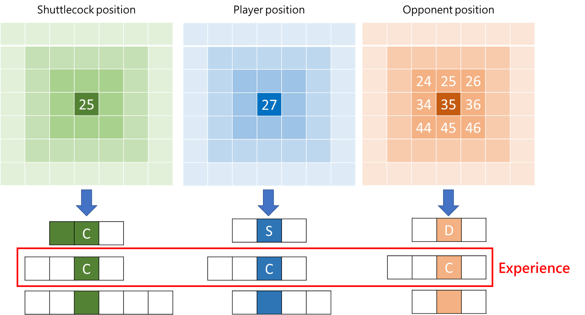
Figure 3: Illustration of the experience extracting function $EXP$.

The experience extraction function $EXP$ identifies historical rallies resembling a given input state, and outputs corresponding action sequences. Before training, we created a dictionary using discrete values for player, opponent, and shuttlecock positions (based on a 10x10 grid) and shot types. This dictionary efficiently stores action sequences for rallies with similar discrete states. When a new state is input, we retrieve matching rallies from the dictionary based on player, opponent, shuttlecock positions, and shot types. The intersected rallies provide experienced combinations, and their action sequences construct the context space. Figure 3 illustrates the experience extraction process. For instance, if the shuttlecock is at position 25, player at 27, opponent at 35, and shot type is clear (denoted as C), we find experiences meeting these conditions. If strict conditions are not met, we expand the range until a fitting experience is found.

Although dictionary retrieval may introduce errors due to relaxed selection criteria, the goal is to establish context spaces for the agent to learn and select appropriate contexts. Balancing the trade-off between error and generalization ability is crucial. A stricter criterion reduces errors but may limit generalization during sparse states, emphasizing the need for effective training to ensure proper context generalization.

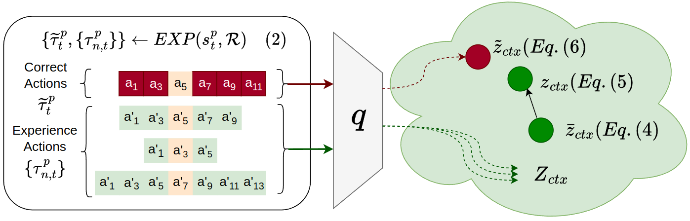
Figure 4: Illustration of Experiential Context Selector (ECS).

Figure 4 illustrates the procedure that ECS constructs the context space and selects contexts as tactical intents based on the extracted experiences. We employ the variational autoencoders (VAE) [17, 18] architecture as the context encoder and context decoder for learning meaningful context representations from experiences. For the $t$-th step in a rally, the context encoder $q$ encodes experiences $\{\tau_{n,t}^{p}\}$ into contexts. The context encoder $q$ encodes the $n$-th experience $\tau_{n,t}^{p}$ into context $z_{n}$:

$$z_{n}\sim q(\bullet|\tau_{n,t}^{p}).$$ (3)

ECS iteratively encodes every experience into a context and collects them as $Z_{ctx}$ for building a context space. Following existing work (e.g., [19, 20]) producing latent representations, we average the collected contexts $Z_{ctx}$ to get the centroid of the context space $\bar{z}_{ctx}$:

$$\bar{z}_{ctx}=mean(Z_{ctx}).$$ (4)

We concatenate the centroid of the context space $\bar{z}_{ctx}$ and state embedding $x_{t}^{p}$ and use a linear layer as the context selector $CTX$ to select the player context $z_{ctx}$ as the agent’s intent:

$$z_{ctx}=CTX(concat(\bar{z}_{ctx},x_{t}^{p})).$$ (5)

As mentioned in Section III-A, there are two processes in ECS: (i) For the $t$-th step in a rally, the player process selects the player context $z_{ctx}$ in the context space constructed based on the experiences; and (ii) The target process utilizes the same context encoder $q$ to encode the correct action sequence of $\widetilde{\tau}_{t}^{p}$ to obtain the target context $\widetilde{z}_{ctx}$:

$$\widetilde{z}_{ctx}\sim q(\bullet|\widetilde{\tau}_{t}^{p}).$$ (6)

Since the goal of the player process is to produce outputs that are close to the target process, the goal of the context selector is to select a player context that is close to the target context.

III-D Latent Geometric Brownian Motion (LGBM)

In badminton games, players consider their opponent’s intent and next action to determine their defensive position accordingly to better receive the shuttlecock. As a result, a player’s behavior changes depending on the opponent’s intent. To enable the agent’s behavior to jointly consider the opponent’s actions, LGBM is proposed to model players as particles undergoing geometric Brownian motion in latent space, which brings the inductive bias of geometric Brownian motion into the player’s decision-making. The successful application of GBM in diverse domains, including finance systems [21] and population dynamics [22], serves as inspiration for its utilization in mitigating uncertainty within turn-based sports. As a continuous-time stochastic process with Gaussian distributed increments, GBM establishes a robust foundation, affording adaptability in mapping the latent space to diverse distributions [23]. This flexibility facilitates the capture of diverse decision distributions, accommodating a range of player strategies.

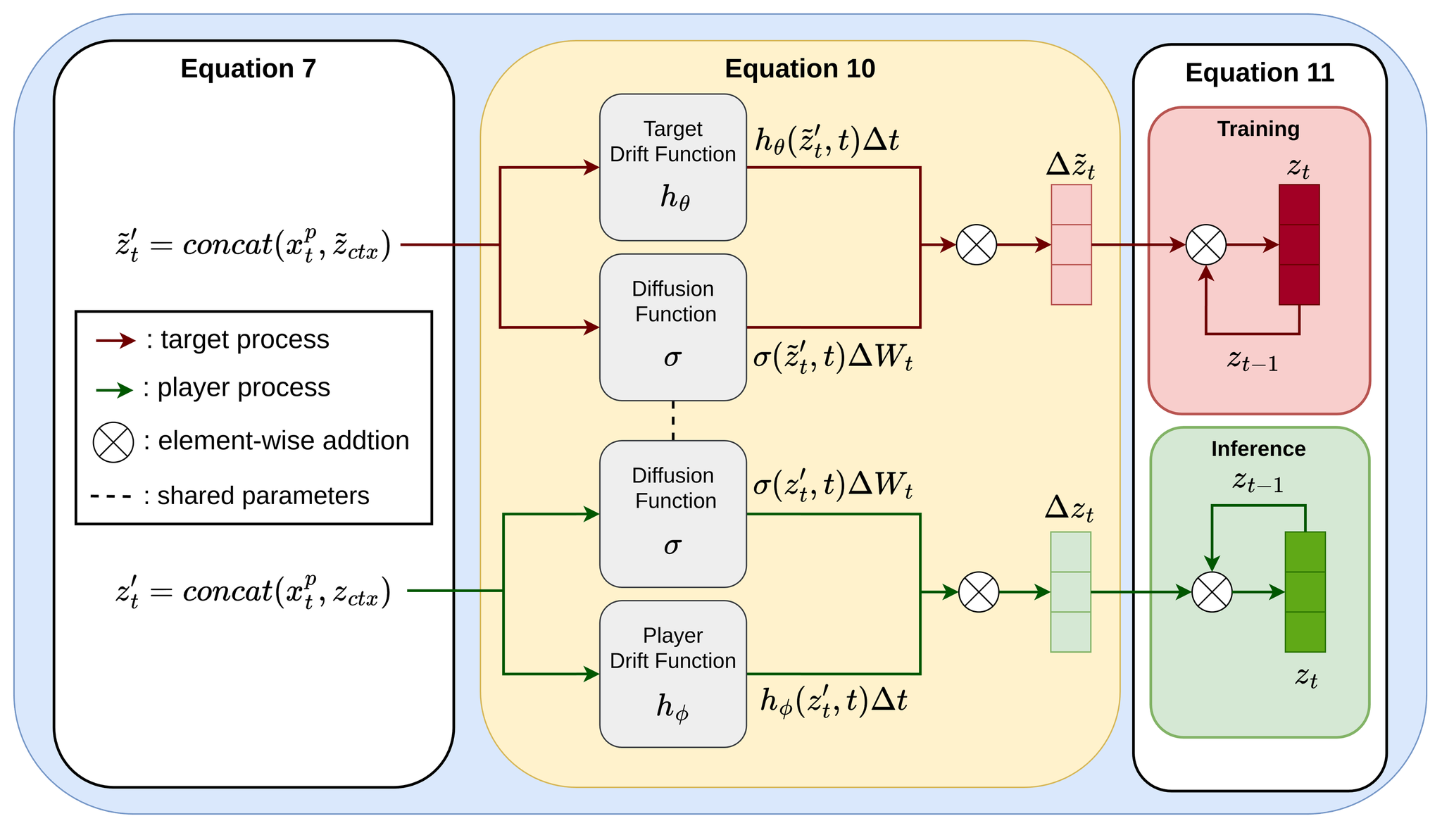
Figure 5: Illustration of Latent Geometric Brownian Motion (LGBM).

Figure 5 demonstrates the alternative simulation of geometric Brownian motion in the latent space in LGBM. This process is driven by the acquired intent from ECS and the player’s rally state. Specifically, we first concatenated the agent’s state and selected context as the agent’s position in the latent space:

$$\begin{split}\widetilde{z}_{t}^{\prime}&=concat(x_{t}^{p},\widetilde{z}_{ctx}),\\ z_{t}^{\prime}&=concat(x_{t}^{p},z_{ctx}),\\ \end{split}$$ (7)

where $\widetilde{z}_{t}^{\prime}$ is the target latent position for the target process and $z_{t}^{\prime}$ is the player latent position for the player process. Secondly, we followed the setting in [24] to simulate the geometric Brownian motion in the latent space. A standard Brownian motion is a random process and is described by the following stochastic differential equation (SDE):

$$dX_{t}=\sigma(x,t)dW_{t},$$ (8)

where $W_{t}$ is Brownian motion and $\sigma$ is the diffusion function. $\mathrm{\Delta}W_{t}\sim\sqrt{\Delta t}\,\mathcal{N}(0,1)$ is used for the simulation of the Brownian motion, where $\mathcal{N}(0,1)$ is a normal distribution with zero mean and unit variance. The geometric Brownian motion can be generalized from Eq. (8) with a drift function $h(x,t)$:

$$dX_{t}=h(x,t)dt+\sigma(x,t)dW_{t}.$$ (9)

We describe the discrete-time SDE of the geometric Brownian motion in the latent space for two processes, $\mathrm{\Delta}\widetilde{z}_{t}$ and $\mathrm{\Delta}z_{t}$ as follows:

$$\begin{split}\mathrm{\Delta}\widetilde{z}_{t}=h_{\theta}(\widetilde{z}_{t}^{\prime},t)\mathrm{\Delta}t+\sigma(\widetilde{z}_{t}^{\prime},t)\mathrm{\Delta}W_{t},\\ \mathrm{\Delta}z_{t}=h_{\phi}(z_{t}^{\prime},t)\mathrm{\Delta}t+\sigma(z_{t}^{\prime},t)\mathrm{\Delta}W_{t},\end{split}$$ (10)

where $h_{\theta}$ and $h_{\phi}$ are the target drift function and the player drift function, respectively. Both processes share the same function $\sigma$. Finally, we add the displacement to the previous latent position to compute the new latent position:

$$\begin{split}z_{t}&=z_{t-1}+\mathrm{\Delta}\widetilde{z}_{t}\enspace\mbox{(during training)},\\ z_{t}&=z_{t-1}+\mathrm{\Delta}z_{t}\enspace\mbox{(during inference)}.\end{split}$$ (11)

Since the displacement can be regarded as the decision of the agent, LGBM makes the agent consider the opponent’s decision through the displacement added to the previous latent position.

III-E Action Projection Layer

The action projection layer is designed to project the latent position to the action that can interact with the opponent. To predict the shot type, we apply a linear layer to the latent position $z_{t}$ to predict the shot type $\hat{t}_{t}^{p}$ at the $t$-th step:

$$\hat{t}_{t}^{p}=softmax(W^{T}z_{t}),$$ (12)

where $W^{T}\in\mathbb{R}^{N_{t}\times d}$ is a learnable matrix, and $N_{t}$ is the number of shot types. To predict the landing positions $\hat{l}_{t}^{p}$ and the moving positions $\hat{m}_{t}^{p}$, we assume the landing distribution and moving distribution are weighted bivariate normal distributions which contain the mean $\{\mu_{t}\}=\{\langle\mu_{x},\mu_{y}\rangle_{t}\}$, standard deviation $\{\sigma_{t}\}=\{\langle\sigma_{x},\sigma_{y}\rangle_{t}\}$, and weight $\{w_{t}\}$ of $N_{g}$ bivariate normal distributions. We apply two linear layers to predict the parameterized distributions for the landing and moving positions:

$$\begin{split}\langle\{\mu_{t}^{L}\},\{\sigma_{t}^{L}\},\{w_{t}^{L}\}\rangle&=W^{L}z_{t},\\ \langle\{\mu_{t}^{M}\},\{\sigma_{t}^{M}\},\{w_{t}^{M}\}\rangle&=W^{M}z_{t},\end{split}$$ (13)

where $W^{L}\in\mathbb{R}^{5\times N_{g}\times d}$ and $W^{M}\in\mathbb{R}^{5\times N_{g}\times d}$ are two learnable matrices for landing and moving, respectively. Finally, we concatenate the shot types and both landing and moving positions to get the action of agent $\hat{a}_{t}^{p}=\langle\hat{t}_{t}^{p},\hat{l}_{t}^{p},\hat{m}_{t}^{p}\rangle$ and decide the next state of the opponent.

III-F Loss Function

To mimic the player’s action at each step, we minimize the loss as:

$$\mathcal{L}=w_{1}\cdot\mathcal{L}_{pred}+w_{2}\cdot\mathcal{L}_{ctx}+w_{3}\cdot\mathcal{L}_{sde},$$ (14)

where $w_{1}$, $w_{2}$, $w_{3}$ $\in$ [0, 1] are hyper-parameters to balance the weights of the corresponding losses.

$$\begin{split}\mathcal{L}_{pred}&=\mathcal{L}_{type}+\mathcal{L}_{land}+\mathcal{L}_{move}+\mathcal{L}_{reg},\\ \mathcal{L}_{type}&=-\sum_{T_{r}\in\{\mathcal{R}\}}\sum_{t=1}^{T}t_{t}^{p}\log\hat{t}_{t}^{p},\end{split}$$ (15)

where $\mathcal{L}_{type}$ is the cross-entropy loss for the predicted shot types. $\mathcal{L}_{land}$ and $\mathcal{L}_{move}$ are the negative log-likelihood losses for the prediction of both landing and moving positions. To simplify the expression, we use $\mathcal{L}_{(land,\ move)}$ to represent $\mathcal{L}_{land}$ or $\mathcal{L}_{move}$:

$$\begin{split}&\mathcal{L}_{(land,\ move)}=-\sum_{T_{r}\in\{\mathcal{R}\}}\sum_{t=1}^{T}\\ \log(&\mathcal{P}(x_{t}^{(L,\ M)},y_{t}^{(L,\ M)}|\{\mu_{t}^{(L,\ M)}\},\{\sigma_{t}^{(L,\ M)}\},\{w_{t}^{(L,\ M)}\})).\end{split}$$ (16)

The regularization loss $\mathcal{L}_{reg}$ is also introduced to prevent the model from degenerating into a simple strategy by ensuring the avoidance of overlapping bivariate normal distributions, computed as the average negative distance between their means.

The context encoder encodes each experience and generates the mean and standard deviation for each context. These values are used to sample the context embedding, which is then passed to the context decoder for experience reconstruction. Therefore, $\mathcal{L}_{ctx}$ consists of the latent loss $\mathcal{L}_{latent}$ and the reconstruction loss $\mathcal{L}_{recon}$. The latent loss $\mathcal{L}_{latent}$ is the KL divergence between the context space distribution and the standard Gaussian distribution $\mathcal{N}(0,1)$ (with zero mean and unit variance). Specifically, $\mathcal{L}_{latent}$ can be expressed as:

$$\mathcal{L}_{latent}=D_{KL}(\mathcal{N}(\mu_{c},\sigma_{c})||\mathcal{N}(0,1)),$$ (17)

where $\mu_{c}$ and $\sigma_{c}$ are the mean and standard deviation output by the context encoder, respectively. The objective of context decoders is to reconstruct intent, which are action sequences of rallies, from selected contexts. Therefore, the reconstruction loss $\mathcal{L}_{recon}$ is the same as $\mathcal{L}_{pred}$, where we minimize the cross-entropy loss for the reconstructed shot types, the negative log-likelihood losses for the reconstructed landing and moving positions, and the average negative distance between the means of bivariate normal distributions.

The player process output needs to be close to the target process as only the player process is used during inferencing. We follow [24] to minimize the KL divergence $\mathcal{L}_{sde}$ between two SDEs in Eq. (10) of LGBM:

$$\mathcal{L}_{sde}=\sum_{T_{r}\in\{\mathcal{R}\}}\sum_{t=1}^{T}\frac{1}{2}\lvert(h_{\phi}(\widetilde{z}_{t}^{\prime},t)-h_{\theta}(\widetilde{z}_{t}^{\prime},t))/\sigma(\widetilde{z}_{t}^{\prime},t)\rvert^{2}.$$ (18)

IV Experiments

To assess RallyNet’s imitation performance, we conducted extensive experiments to address the alignment with the three key criteria and delved into three additional research questions, aiming to comprehensively evaluate RallyNet’s effectiveness and its value to the badminton community:

• Behavioral Sequence Similarity: Do the sequences of shot types, shuttlecock landing positions, and player moving positions in rallies generated by RallyNet closely match those in real rallies?

• Rally Duration Realism: Does RallyNet accurately replicate the length of rallies, providing a realistic representation of the duration observed in real matches?

• Outcome Consistency: Are the outcomes of rallies generated by RallyNet consistent with the real-world results? Specifically, does the win rate of rallies simulated by the learned agent align with the win rate of real players?

• Ablation Studies: Does each component of RallyNet affect the prediction results?

• Sensitivity Analysis: How sensitive is RallyNet’s performance to variations in input parameters and conditions?

• Case Studies: How does RallyNet’s capability to replicate player behavior bring valuable applications to the badminton community?

IV-A Experimental Setup

IV-A1 Badminton Dataset

RallyNet is evaluated on the largest badminton singles dataset, which is the only publicly available benchmark in turn-based sports [9, 25]. This dataset comprises 75 singles matches played by 31 players from 2018 to 2021, totaling 180 sets, 4,325 rallies, and 43,191 strokes. To construct the action space, we used the 12 shot types defined by [26], namely receiving, short service, long service, net shot, clear, push/rush, smash, defensive shot, drive, lob, drop, and can’t reach. The range of each dimension of the badminton court was rescaled to [-1,1] to ensure that the model would not be affected by different ranges. We trained our model on the first 80% of the rallies, and the remaining 20% of rallies were used to evaluate the performance of our model as well as the 5-fold cross-validation for tuning the hyper-parameters.

IV-A2 Baselines

We compared RallyNet against several baselines, including:

• Random agent, which samples the shot type as well as both the landing and moving positions uniformly randomly.

• Rule-based agent, which samples from the distribution of the shot type and from both landing and moving distributions which are obtained through the experience extracting function of RallyNet.

• IQ-Learn [27], a state-of-the-art model-free offline inverse reinforcement learning algorithm.

• Behavior Cloning (BC) [28], which learns a mapping from a state to an action.

• Hierarchical Behavioral Cloning (HBC) [29], which learns an options-type hierarchical policy from expert demonstrations.

• ShuttleNet [9], which is a specialized model designed for stroke forecasting. It fuses the contexts of rally progress and player styles to predict the shot type and the landing position based on past information. It is noted that ShuttleNet requires at least two steps to encode players’ contexts; therefore, it cannot be tested only on the initial state. Since ShuttleNet originally predicted only the shot type and landing positions, we extended its capabilities by incorporating a module similar to the landing position prediction to also enable the prediction of moving positions.

• DyMF [25], which is a specialized model designed for badminton movement forecasting. It employs interaction style extractors to adeptly capture nuanced player interactions and evolving tactics across rallies. DyMF predicts players’ shot types and movements. Given that a player’s receiving position essentially determines the landing spot, DyMF seamlessly aligns with our problem setting. However, akin to ShuttleNet, DyMF relies on at least two steps of past information for future predictions, limiting its capacity to recover the entire rally from an initial state.

IV-A3 Implementation Details

To avoid the agent’s predictions for landing positions and movement positions encompassing the entire court and degenerating the strategy, we imposed a constraint on the standard deviation of the bivariate Gaussian distribution for our method and all baselines. The standard deviation was limited to the range of [-0.1, 0.1]. To improve the model’s generalization capability and to mitigate over-reliance on experiences for decision-making, we utilized an experience extracting function that restricted the number of experiences for the current state to 5. This was done because a substantial amount of experience cannot be guaranteed during testing, particularly in the later stages of a turn-based setting when the states become sparse.

The dimension of state embedding was set to 80, and the dimension of context embedding was set to 128. The batch size was 32 and the number of training epochs was 100 using Adam optimizer. The learning rate was set to 0.0001. For HBC implementations, the number of options for HBC was treated as a hyperparameter, with experiments conducted using various numbers of options 2, 4, 8, 16. The optimal result was observed when the number of options was set to 4. All training and evaluation experiments were performed on a machine equipped with an Intel i7-8700 3.2GHz CPU, Nvidia GTX 3060 12GB GPU, and 32GB RAM.

TABLE I: Quantitative results. The best is in boldface and the second best is underlined. Since ShuttleNet and DyMF predict based on past information, the symbol $-$ denotes that the result is unavailable.

	Given initial state only				Given states of the first two steps
Model	Land($\downarrow$)	Shot($\downarrow$)	Move($\downarrow$)	MRNS($\uparrow$)	Land($\downarrow$)	Shot($\downarrow$)	Move($\downarrow$)	MRNS($\uparrow$)
Random agent	1.3044	104.382	0.8506	-	1.2548	79.2586	0.8763	-
Rule-based agent	0.9130	65.4033	0.5942	1	1.0888	61.7431	0.6464	1
IQ-Learn [27]	1.7464	127.8784	1.072	-0.8652	1.6454	112.0538	1.0555	-1.6682
BC [28]	0.9603	63.5967	0.4829	1.1199	1.0343	56.1007	0.5832	1.3084
HBC [29]	0.6940	32.5972	0.4031	1.7155	0.8760	33.1886	0.5529	2.1062
DyMF [25]	-	-	-	-	1.1828	26.5931	1.2266	0.6389
ShuttleNet [9]	-	-	-	-	0.9090	34.0467	0.5059	2.0918
RallyNet (Ours)	0.5931	18.8678	0.3416	1.9988	0.7959	19.5100	0.4943	2.6124

IV-A4 Evaluation Metrics

Given the absence of prior research on the imitation of behaviors in turn-based sports, we proposed 4 evaluation metrics to measure the similarity between generated rallies and true player rallies. To evaluate the results of shot type prediction, we used Connectionist Temporal Classification (CTC) loss [30] for uncertainty measurement, which is defined as the negative log-likelihood of the labels given input sequences. To evaluate the results of the predicted landing and moving positions, we used Dynamic Time Warping (DTW) [31] to calculate the distance between generated position sequence and the true position sequence, which can assess the similarity of two sequences at a global level, as used recently in [32, 33]. Using the DTW distance and the CTC loss has the benefit that the similarity of two sequences can be assessed even if each sequence is of a different length. Moreover, inspired by [34, 35], we further provide an overall comparison of the algorithms by introducing a metric termed Rule-based agent Normalized Score (RNS) defined as:

$$RNS=\frac{(Random_{score}-Agent_{score})}{(Random_{score}-Rule_{score})},$$ (19)

where the subscript $score$ indicates the metric used and can be either DTW distance or CTC loss, and $Agent_{score}$ is the performance of the agent. $Random_{score}$ and $Rule_{score}$ are the performance of the random agent and the rule-based agent, respectively.

To provide an overall comparison of the algorithms, we present the Mean RNS (MRNS), which is defined as the average over the RNS values under the three base metrics. This metrics selection aligns with our emphasis on tactical execution, a domain where conventional metrics like Mean Squared Error (MSE) or Cross-Entropy (CE) used in [9, 25] fail to reflect the intricate similarities inherent in decision sequences. This limitation becomes evident when minor sequence deviations arise. For instance, even if a strategy compels opponents to traverse the court substantially, a minor delay by a single stroke should still be recognized as similar. All the results are the average of 5 different random seeds.

IV-B Quantitative Results (RQ1)

Table I presents the performance of RallyNet and the baselines. We summarize the observations as follows:

IV-B1 Superior Performance of RallyNet

Clearly, RallyNet surpasses all the baselines in terms of all metrics, whether given only the initial state, or the state of the first two steps. Quantitatively, RallyNet outperforms all the baselines by at least 7.08 in terms of CTC loss when predicting the shot types, and achieves lower DTW distances than the baselines by at least 8.27% and 1.16% in the predicted landing and moving positions, respectively. Note that since players usually have similar positions and shot types for serving and receiving (i.e., the first two steps), the prediction after two steps is more difficult to predict. These results demonstrate that RallyNet addresses the compounding error in offline imitation learning for turn-based sports well.

IV-B2 Hierarchical BC Advantage

We observe that IQ-Learn produces unfavorable performance, possibly due to the difficulty of inferring the reward function in a scenario where the opponent exclusively determines the next state. This may lead to a weak correlation between the current and the next state, making IQ-Learn unsuitable for this particular task. HBC can better capture complex player strategies as it can switch between different strategies by selecting different options based on the different states. We can observe that HBC achieves better prediction than BC, and manifests the importance of using HIL in the turn-based setting.

IV-B3 The Importance of Leveraging Experience

Existing supervised learning methods for turn-based sports, such as ShuttleNet and DyMF, diverge from imitation learning models. These models, structured on sequence-to-sequence architectures, predict player actions by relying on historical rally data. DyMF excels in predicting shot types, while ShuttleNet performs well in forecasting player movements, showcasing its proficiency in the handling of player interactions and rally dynamics. However, these approaches face challenges as errors accumulate during extended rallies. In contrast, RallyNet stands out by leveraging experience, enabling it to emulate player-like behavior even in prolonged rallies. This distinctive capability serves to alleviate the cumulative errors observed in other methods, resulting in more realistic and accurate behavioral predictions.

IV-C Length Distribution Difference (RQ2)

The length of generated rallies serves as a reflective measure of whether the model has learned realistic gameplay situations. A model capable of capturing rally duration can reflect a genuine simulation of the match. To visually depict the distribution of generated rally lengths in comparison to real rally lengths, we utilize Kernel Density Estimate (KDE). Additionally, the quantitative dissimilarity between these two distributions is evaluated using the Jensen–Shannon divergence (JSD). In Figure 6, BC struggles to effectively capture player interactions, resulting in premature or delayed termination. In contrast, both HBC and RallyNet, by modeling more intricate strategies, produce generated rally length distributions close to the real ones. Notably, even a rule-based agent using our carefully designed experience extraction function can achieve a similar rally length distribution, emphasizing that our experience extraction captures rally duration to aid RallyNet in making more realistic decisions. Figure 7 depicts the generated length distributions of ShuttleNet and DyMF alongside real ones. It is evident that ShuttleNet and DyMF, not being imitation learning models but sequence-to-sequence tasks, face the challenge in generating ideal rally lengths. This challenge stems from the infrequent occurrence of error behaviors in dataset, where a rally involves only one error behavior (e.g., shuttlecock out of bounds or hitting the net), posing a significant obstacle for these models to accurately capture rally duration.

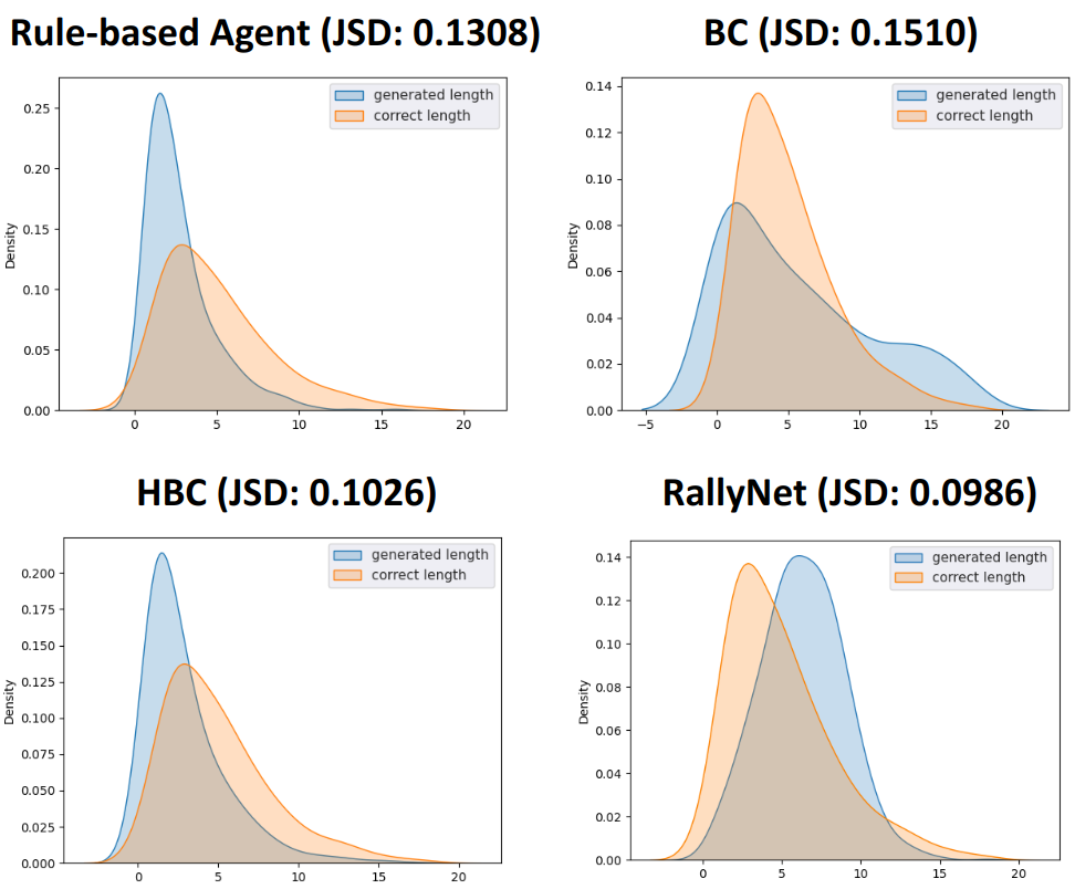
Figure 6: The length distribution difference. The orange distribution represents the ground truth rally length distribution, while the blue distribution depicts the generated rally length distribution.

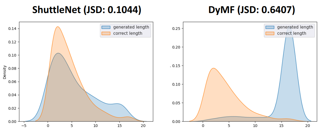
Figure 7: The length distribution difference between generated rallies and ground truth rallies. It is evident that existing sequence-to-sequence methods struggle to capture the timing of player error behavior.

IV-D Win Rate Difference (RQ3)

To evaluate the outcome consistency of learned models in mimicking real player behavior, we adopt a straightforward approach by examining win rates among players. As depicted in Table II, considering the diverse quantities of match data available for each player in the dataset, our analysis focuses on two real-world professional players, X and Y, who possess the most extensive match records. For both X and Y, we chose four opponents from their respective match histories, subsequently comparing the generated rally win rates with the simulated win rates from the models.

To ensure the validity of win rate observations within realistic gameplay scenarios, we evaluated the performance of the top three imitation learning models: BC, HBC, and RallyNet. Table II illustrates that RallyNet consistently demonstrates smaller differences from the actual win rate across a majority of matchups, with a maximum difference of merely 8.15% and an average difference of 3.79%. In contrast, BC and HBC exhibit differences of up to 22.5% in specific matchup combinations, with an average difference surpassing RallyNet by at least 7.16%. These findings not only underscore RallyNet’s stability but also highlight its exceptional capability to accurately replicate real match outcomes.

TABLE II: Win rate differences between ground truths and learned agents. X and Y denote two actual players chosen from the dataset. A, B, C, D are the four opponents of player X, while E, F, G, H are the four opponents of player Y, selected from their past matches. Lower differences indicate better alignment between the observed win rates and those predicted by the learned agents.

	X				Y
Opponent	A	B	C	D	E	F	G	H	Mean Difference
Ground Truth Win Rate	0.4406	0.5760	0.6250	0.5945	0.5416	0.4000	0.5454	0.4615	-
BC	0.1413	0.0508	0.1042	0.0810	0.2084	0.2000	0.1364	0.1923	0.1393
HBC	0.0806	0.1316	0.0773	0.0493	0.0153	0.2250	0.0749	0.2227	0.1095
RallyNet (Ours)	0.0760	0.0000	0.0208	0.0810	0.0416	0.0000	0.0455	0.0385	0.0379

TABLE III: Ablation study of our model.

	Given initial state only				Given states of first two steps
Model	Land($\downarrow$)	Shot($\downarrow$)	Move($\downarrow$)	MRNS($\uparrow$)	Land($\downarrow$)	Shot($\downarrow$)	Move($\downarrow$)	MRNS($\uparrow$)
BC	0.9603	63.5967	0.4829	1.1199	1.0343	56.1007	0.5832	1.3084
BC w/ ECS	0.6877	27.0127	0.4577	1.6976	0.9259	29.4051	0.5780	2.0416
Indiv. RallyNet	0.6063	19.0623	0.3766	1.9404	0.8189	21.3749	0.5305	2.4782
RallyNet (Ours)	0.5931	18.8678	0.3416	1.9988	0.7959	19.5100	0.4943	2.6124

IV-E Ablation Studies (RQ4)

As RallyNet can be seen as an extension of BC with the addition of ECS and LGBM, an ablation study was conducted by developing two variants to investigate the relative contributions of two components: 1) BC w/ ECS, which is RallyNet without the LGBM module, 2) Indiv. RallyNet, which is RallyNet with the proposed LGBM replaced by the individual LGBMs (i.e., two independent stochastic processes, one for each player). The result is shown in Table III.

IV-E1 The Effect of ECS

Recall that ECS was designed to capture the agent’s intent through experience, enabling the agent’s behavior throughout the rally to not be influenced by partially incorrect decisions. The agent can already achieve a moderately low prediction error by adding ECS to BC, especially when predicting the shot type and the landing position. However, without the help of LGBM, the agent suffers from a large error in moving position since it disregards the opponent’s behavior.

IV-E2 The Effect of LGBM

Recall that LGBM is meant to jointly capture the interaction of players to help the agent generate more realistic behavior. RallyNet (i.e., BC w/ ECS w/ LGBM) demonstrates a significant improvement in performance, particularly in the prediction of moving positions, compared to the model BC w/ ECS. Furthermore, we investigated the effect of replacing the proposed LGBM with individual LGBMs (i.e., Indiv. RallyNet). The results showed that without the shared inductive bias introduced by proposed LGBM, the agent ignored players’ interaction, resulting in a degradation of the predicted moving position performance. Overall, the results further support the effectiveness of LGBM in RallyNet and provide evidence that RallyNet captures the alternative decision-making nature of the turn-based sports.

IV-F Sensitivity Analysis (RQ5)

IV-F1 Loss weights

The loss that we are minimizing is:

$$\mathcal{L}=w_{1}\cdot\mathcal{L}_{pred}+w_{2}\cdot\mathcal{L}_{ctx}+w_{3}\cdot\mathcal{L}_{sde},$$ (20)

where $w_{1}$, $w_{2}$, $w_{3}$ $\in$ [0, 1] are hyper-parameters to balance the weights of the corresponding losses. We have set the loss weights $w_{1},w_{2},w_{3}$ to 1. Considering the significant scale difference between $\mathcal{L}_{land}$, $\mathcal{L}_{move}$, and $L_{reg}$ compared to $\mathcal{L}_{type}$, we scale down $\mathcal{L}_{land}$, $\mathcal{L}_{move}$, and $\mathcal{L}_{reg}$ by a factor of 0.01. The purpose of $\mathcal{L}_{reg}$ is to add a regularization loss that prevents overlap between the predicted landing distributions and moving distributions, ensuring that the model does not degenerate into a simple policy. This regularization loss is defined as the average negative distance between bivariate normal distributions. The relationship between $\mathcal{L}_{type}$, $\mathcal{L}_{land}$, $\mathcal{L}_{move}$, and $\mathcal{L}_{reg}$ is given by:

$$\mathcal{L}_{pred}=\mathcal{L}_{type}+\frac{(1-\alpha)}{100}\cdot\mathcal{L}_{(land,move)}+\frac{\alpha}{100}\cdot\mathcal{L}_{reg},$$ (21)

where the regularization loss weight $\alpha$ is set to 0.05 for all experiments. To investigate the influence of varying loss weights on the model’s performance, we conducted a parameter analysis by examining different values for $w_{1}$, $w_{2}$, and $w_{3}$. Specifically, we evaluated the model’s MRNS using weights of 0.25, 0.50, and 0.75 for each loss term. The results of these experiments are presented in Figure 8.

The results indicate that increasing the weights of $\mathcal{L}_{pred}$ and $\mathcal{L}_{ctx}$ improves performance by enhancing the accuracy of target process outputs and context representation learning. This enables the player process used for inference to closely approximate the precise target process. We also observed that the influence of $\mathcal{L}_{sde}$ on performance is stable. This suggests that when the target process is effectively learned, the player process effortlessly approximates the target process, resulting in consistent performance that is minimally affected by $\mathcal{L}_{sde}$.

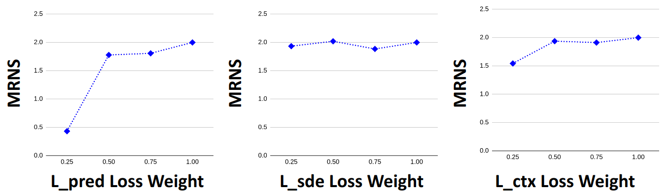
Figure 8: MRNS Performance of RallyNet w.r.t different value of loss weights.

IV-F2 Context dimension

In all experiments, we set the context embedding dimension to 128. The dimension of the context embedding plays a crucial role in determining the continuity of the context space and influencing the specificity of the selected context (i.e., player’s intention). As shown in Figure 10, increasing the dimension of the context embedding results in improved overall performance.

IV-F3 The number of bivariate Gaussian distributions

Across all experiments, we utilized a fixed number of 5 bivariate Gaussian distributions for predicting landing positions and moving positions. The number of distributions played a crucial role in the accuracy of these predictions. We conducted experiments with three different numbers of bivariate Gaussian distributions: 2, 5, and 8. Figure 10 reveals that insufficient or excessive distributions were unable to adequately capture the intricate distributions of landing positions and moving positions.

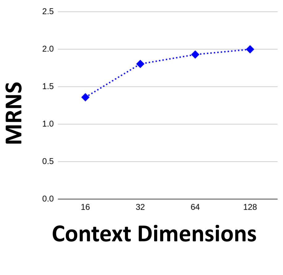
Figure 9: MRNS Performance of RallyNet w.r.t different value of context dimensions.

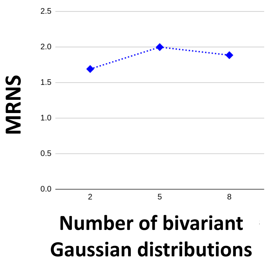
Figure 10: MRNS Performance of RallyNet w.r.t different number of distributions

IV-F4 Cross-Domain Evaluation

We cannot test our model on other turn-based sports since there is only one existing public dataset that can be accessed. To further illustrate the effectiveness of RallyNet, we have included additional experiments by comparing RallyNet with our baselines in the Pong environment of Atari games, which shares some turn-based characteristics. The state of the Pong environment is an image, and the action is a discrete one that includes left and right movement. To train an expert, we used DQN and captured the position of each shot of the agent and the computer opponent simultaneously. We then converted the data into those of the same turn-based data format as our badminton dataset, including landing position, moving position, and whether the ball is reachable. We also rescaled the court to between -1 and 1. Regarding RallyNet on Pong, we used the same implementation as that for badminton. It is worth mentioning that ShuttleNet and DyMF have the limitation wherein they require information of the previous two steps to make predictions. Thus, they cannot be directly compared to RallyNet and the baselines of imitating rally-wise player behavior. Table IV illustrates the comparative results of imitating player behavior in the Pong environment. The results show that RallyNet outperforms all the baselines and indicate that RallyNet can address the compounding error in offline imitation learning for other turn-based sports environments.

TABLE IV: Quantitative results on the Pong environment of Atari games.

	Given initial state only			Given states of first two steps
Model	Land	Shot	Move	Land	Shot	Move
BC	0.4025	5.2086	0.5764	0.4859	1.5431	0.5618
HBC	0.4079	4.5921	0.4787	0.4960	0.6891	0.5162
RallyNet	0.3884	4.4488	0.4495	0.4513	0.5738	0.4764

IV-G Case Studies (RQ6)

IV-G1 Simulation of Player Behavior

We describe a use case of the learned model in sports analytics for characterizing the style of a professional player by simulating the behavior of the player (e.g., the landing and the subsequent moving position upon a shot) against different opponent players in different scenarios. Figure 11 shows the simulated distributions of the landing and moving position of a player after a defensive shot. In this example: (i) This player tends to have a landing position mostly on both sides of the backcourt and only occasionally on the midcourt. (ii) This player tends to move to the midcourt after a defensive shot to prepare for the next stroke.

To provide a more comprehensive view of the results, we have generated visualizations comparing the landing distributions of RallyNet and BC across various states. Figure 12 illustrates the simulated landing distributions of under different state conditions. It demonstrates that RallyNet consistently captures players’ decision patterns with precision. In contrast, BC exhibits instances where it manages to approximate the distribution roughly but with deviations, and occasionally even exhibits significant misjudgments. Accordingly, such characterization can help the coach better understand the style of the player and thereby devise tactical plans.

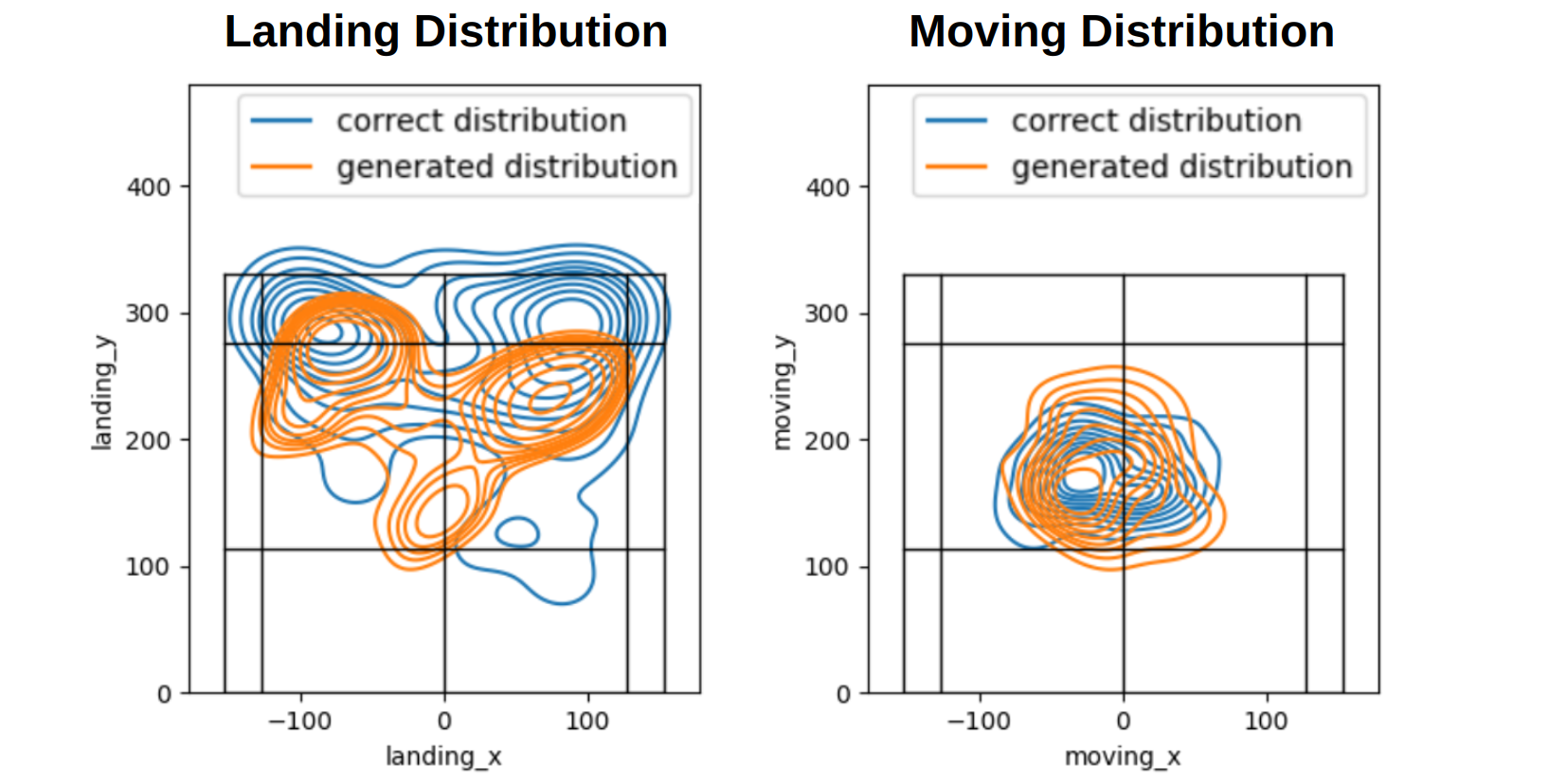
Figure 11: The landing distributions and the moving distributions of a player when using a defensive shot.

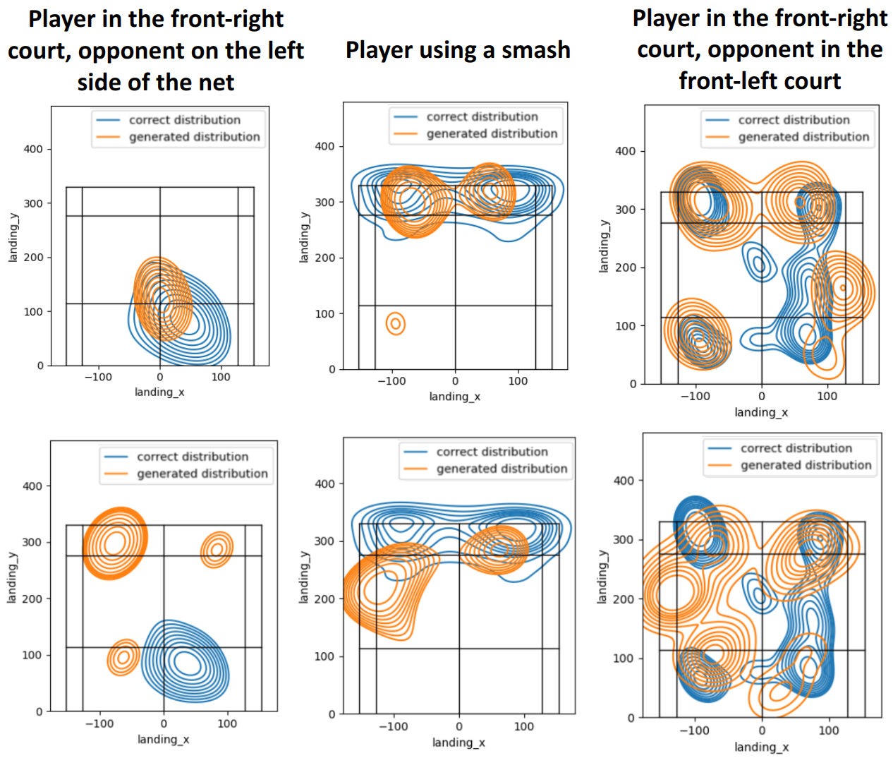
Figure 12: The landing distributions of the player in various states are shown, with RallyNet in the upper row and BC in the lower row. RallyNet excels in capturing landing distribution compared to BC. Note that these visualizations portray results extracted from the testing dataset corresponding to each specific state, not the model’s predicted landing distribution for a specific state.

IV-G2 Tactical Interpretation of Player Behavior

RallyNet strategically interprets player behavior by selecting a context as the agent’s intent, guiding its actions accordingly. The intent is decoded by the context decoder of the ECS, revealing the expected action sequence. Figure 13 exemplifies this process, deciphering the intent behind a shot based on the preceding (long serve in the green grid) and current shots (net shot in the yellow grid). For instance, if Player A’s intent is decoded as planning a subsequent smash by strategically positioning the opponent in the backcourt, it suggests a tactical move to set up aggressive shot returns. This showcases RallyNet’s capability to provide insightful tactical interpretations, a valuable asset for badminton coaches and players.

To validate the system’s ability to decode the physical meaning of selected contexts, we conducted a reconstruction experiment. This evaluated the reconstruction performance of the context decoder in ECS, showcasing its effectiveness in terms of capturing the player’s intent from their actions. Unlike focusing on player interactions, this approach directly extracts the underlying intent from the action sequence. Table V demonstrates that the reconstruction performance surpasses the imitation performance, showcasing the effectiveness of our context encoder in capturing and decoding player intent.

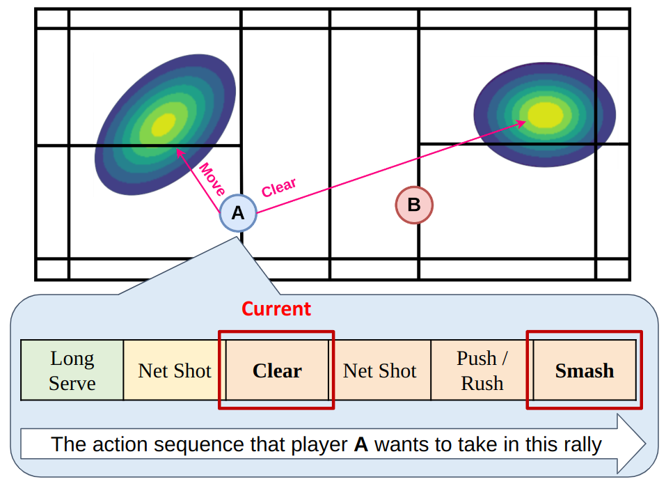
Figure 13: An example of interpreting the intent behind a player’s action. The clear stroke by player A is meant to plan for a subsequent smash.

TABLE V: The reconstruction performance of the context encoder.

Model	Land($\downarrow$)	Shot($\downarrow$)	Move($\downarrow$)
RallyNet (Ours)	0.4011	4.1918	0.2009

V Related Work

V-A Inverse Reinforcement Learning

Inverse Reinforcement Learning (IRL) [36, 37, 38] is an IL approach that attempts to learn the underlying rewards that an expert is optimizing from the demonstrations. With the learned reward function, IRL can guide the agent’s behavior toward that of the expert. However, in turn-based sports, each player’s actions determine the next state for other players. Treating opponents as part of the environment is equivalent to training in a constantly changing environment, which can make it challenging for IRL to learn optimal policies.

V-B Offline Imitation Learning via Behavior Cloning

Behavior cloning (BC) provides a form of supervised learning for training policies by learning direct mapping from states to actions, which can be used in the offline setting [28, 39]. Recent works such as DT [40], GCSL [41], and RvS [42] have shown that not only is supervised learning and bypassing the learning reward function able to attain better results for offline learning, but it is also easier to use and is more stable than offline inverse reinforcement learning (IRL) [36, 43, 27]. Moreover, previous work [44, 29] has extended the BC to hierarchical BC by dividing a task into several sub-tasks, where the low-level behaviors are controlled by high-level decisions to capture long-term decision-making processes. However, these existing approaches focus on the complex behavior and the long-term task of the same target, but neglect the characteristics of the mixed sequences, which causes serious compounding errors.

V-C Badminton Tactical Analysis

AI has significantly contributed to the domain of badminton sports analytics, addressing diverse challenges. For instance, [45] introduced the Badminton Language for Sequence Representation (BLSR), presenting a unified language capable of efficiently converting match videos into analyzable datasets. BLSR, characterized by its human-readable, universal, and professional nature, enables the straightforward interpretation of entire match processes without the need for video footage. In strokes forecasting, [9] advanced the prediction of players’ future strokes based on their past actions. The innovative ShuttleNet framework incorporates a position-aware fusion of rally progress and player styles, accounting for dependencies at each stroke. Additionally, [25] addressed the movement forecasting task, encompassing stroke and player movement predictions. They employed DyMF, a novel model based on dynamic graphs and hierarchical fusion grounded in player movement graphs. However, past models focused on predicting future actions given specific initial steps, but the lack of realistic agents hampers accurate match simulation. We propose a closed-loop AI approach [1]. This system includes six key components to enhance badminton players’ performance: Badminton Data Acquisition, Imitating Players’ Style, Simulating Matches, Optimizing Strategies, Training Execution, and Real-World Competitions. In this paper, we only focus on one specific task within the closed-loop AI approach: imitating players’ styles. We propose RallyNet to imitate badminton players’ styles. Beyond evaluating RallyNet using previously proposed offline metrics [1], we assess the learned agent’s applicability to different badminton scenarios, confirming the feasibility of RallyNet in badminton games simulation.

VI Conclusion

In this work, we present RallyNet, a novel hierarchical offline imitation learning model for learning player decision-making strategies in turn-based sports. By modeling players’ decision-making processes as CMDP, we introduce ECS which leverages experiences to construct a context space, and selects the context as the agent’s intent. This reduces the impact of partial decision errors on overall behavior. The ECS component reduces decision-making errors of agents in the CMDP setting, even if it is not turn-based, while LGBM captures player interactions to generate more realistic behaviors for various turn-based sports. We believe that the innovative ideas, connecting player intents with interaction models using GBM and offering an understanding of real interactions in turn-based sports, have substantial potential to inspire researchers across other turn-based sports. Our evaluation of a real-world badminton dataset shows that RallyNet outperforms existing offline IL and the state-of-the-art turn-based supervised method, and has potential for sports analytics. Furthermore, we demonstrate that RallyNet is indeed a promising solution to sports analytics via practical use cases.

References

- [1] K.-D. Wang, “Enhancing badminton player performance via a closed-loop ai approach: Imitation, simulation, optimization, and execution,” in Proceedings of the 32nd ACM International Conference on Information and Knowledge Management, ser. CIKM ’23. New York, NY, USA: Association for Computing Machinery, 2023, p. 5189–5192. [Online]. Available: https://doi.org/10.1145/3583780.3616001
- [2] E. Bronstein, M. Palatucci, D. Notz, B. White, A. Kuefler, Y. Lu, S. Paul, P. Nikdel, P. Mougin, H. Chen et al., “Hierarchical model-based imitation learning for planning in autonomous driving,” in 2022 IEEE/RSJ International Conference on Intelligent Robots and Systems (IROS). IEEE, 2022, pp. 8652–8659.
- [3] A. Singh, E. Jang, A. Irpan, D. Kappler, M. Dalal, S. Levinev, M. Khansari, and C. Finn, “Scalable multi-task imitation learning with autonomous improvement,” in 2020 IEEE International Conference on Robotics and Automation (ICRA). IEEE, 2020, pp. 2167–2173.
- [4] D. Zhang, Q. Li, Y. Zheng, L. Wei, D. Zhang, and Z. Zhang, “Explainable hierarchical imitation learning for robotic drink pouring,” IEEE Transactions on Automation Science and Engineering, 2021.
- [5] Y. Gao, B. Shi, X. Du, L. Wang, G. Chen, Z. Lian, F. Qiu, G. Han, W. Wang, D. Ye et al., “Learning diverse policies in moba games via macro-goals,” Advances in Neural Information Processing Systems, vol. 34, pp. 16 171–16 182, 2021.
- [6] H. M. Le, P. Carr, Y. Yue, and P. Lucey, “Data-driven ghosting using deep imitation learning,” 2017.
- [7] W.-Y. Wang, T.-F. Chan, H.-K. Yang, C.-C. Wang, Y.-C. Fan, and W.-C. Peng, “Exploring the long short-term dependencies to infer shot influence in badminton matches,” in 2021 IEEE International Conference on Data Mining (ICDM). IEEE, 2021, pp. 1397–1402.
- [8] J. Won, D. Gopinath, and J. Hodgins, “Control strategies for physically simulated characters performing two-player competitive sports,” ACM Transactions on Graphics (TOG), vol. 40, no. 4, pp. 1–11, 2021.
- [9] W.-Y. Wang, H.-H. Shuai, K.-S. Chang, and W.-C. Peng, “Shuttlenet: Position-aware fusion of rally progress and player styles for stroke forecasting in badminton,” in Proceedings of the AAAI Conference on Artificial Intelligence, vol. 36, no. 4, 2022, pp. 4219–4227.
- [10] S. Giancola and B. Ghanem, “Temporally-aware feature pooling for action spotting in soccer broadcasts,” in IEEE Conference on Computer Vision and Pattern Recognition Workshops, CVPR Workshops 2021, virtual, June 19-25, 2021. Computer Vision Foundation / IEEE, 2021, pp. 4490–4499.
- [11] E. Zhan, S. Zheng, Y. Yue, L. Sha, and P. Lucey, “Generative multi-agent behavioral cloning,” CoRR, vol. abs/1803.07612, 2018. [Online]. Available: http://arxiv.org/abs/1803.07612
- [12] L. Wang, R. Tang, X. He, and X. He, “Hierarchical imitation learning via subgoal representation learning for dynamic treatment recommendation,” in Proceedings of the Fifteenth ACM International Conference on Web Search and Data Mining, 2022, pp. 1081–1089.
- [13] M. Jing, W. Huang, F. Sun, X. Ma, T. Kong, C. Gan, and L. Li, “Adversarial option-aware hierarchical imitation learning,” in International Conference on Machine Learning. PMLR, 2021, pp. 5097–5106.
- [14] A. Hallak, D. Di Castro, and S. Mannor, “Contextual markov decision processes,” arXiv preprint arXiv:1502.02259, 2015.
- [15] D. Revuz and M. Yor, Continuous martingales and Brownian motion. Springer Science & Business Media, 2013, vol. 293.
- [16] M. L. Puterman, Markov decision processes: discrete stochastic dynamic programming. John Wiley & Sons, 2014.
- [17] D. P. Kingma and M. Welling, “Auto-encoding variational bayes,” arXiv preprint arXiv:1312.6114, 2013.
- [18] D. J. Rezende, S. Mohamed, and D. Wierstra, “Stochastic backpropagation and approximate inference in deep generative models,” in International conference on machine learning. PMLR, 2014, pp. 1278–1286.
- [19] M. Garnelo, D. Rosenbaum, C. Maddison, T. Ramalho, D. Saxton, M. Shanahan, Y. W. Teh, D. Rezende, and S. A. Eslami, “Conditional neural processes,” in International conference on machine learning. PMLR, 2018, pp. 1704–1713.
- [20] W. Hamilton, Z. Ying, and J. Leskovec, “Inductive representation learning on large graphs,” Advances in neural information processing systems, vol. 30, 2017.
- [21] K. Reddy and V. Clinton, “Simulating stock prices using geometric brownian motion: Evidence from australian companies,” Australasian Accounting, Business and Finance Journal, vol. 10, no. 3, pp. 23–47, 2016.
- [22] S. Engen, “Stochastic growth and extinction in a spatial geometric brownian population model with migration and correlated noise,” Mathematical Biosciences, vol. 209, no. 1, pp. 240–255, 2007.
- [23] F. Jin, R. P. Khandpur, N. Self, E. Dougherty, S. Guo, F. Chen, B. A. Prakash, and N. Ramakrishnan, “Modeling mass protest adoption in social network communities using geometric brownian motion,” in Proceedings of the 20th ACM SIGKDD International Conference on Knowledge Discovery and Data Mining, ser. KDD ’14. New York, NY, USA: Association for Computing Machinery, 2014, p. 1660–1669. [Online]. Available: https://doi.org/10.1145/2623330.2623376
- [24] X. Li, T.-K. L. Wong, R. T. Q. Chen, and D. Duvenaud, “Scalable gradients for stochastic differential equations,” International Conference on Artificial Intelligence and Statistics, 2020.
- [25] K. Chang, W. Wang, and W. Peng, “Where will players move next? dynamic graphs and hierarchical fusion for movement forecasting in badminton,” in AAAI. AAAI Press, 2023, pp. 6998–7005.
- [26] W. Wang, T. Chan, H. Yang, C. Wang, Y. Fan, and W. Peng, “How is the stroke? inferring shot influence in badminton matches via long short-term dependencies,” ACM Trans. Intell. Syst. Technol., vol. 14, no. 1, 2022.
- [27] D. Garg, S. Chakraborty, C. Cundy, J. Song, and S. Ermon, “Iq-learn: Inverse soft-q learning for imitation,” Advances in Neural Information Processing Systems, vol. 34, pp. 4028–4039, 2021.
- [28] D. A. Pomerleau, “Alvinn: An autonomous land vehicle in a neural network,” Advances in neural information processing systems, vol. 1, 1988.
- [29] Z. Zhang and I. Paschalidis, “Provable hierarchical imitation learning via em,” in International Conference on Artificial Intelligence and Statistics. PMLR, 2021, pp. 883–891.
- [30] A. Graves, S. Fernández, F. Gomez, and J. Schmidhuber, “Connectionist temporal classification: labelling unsegmented sequence data with recurrent neural networks,” in Proceedings of the 23rd international conference on Machine learning, 2006, pp. 369–376.
- [31] D. J. Berndt and J. Clifford, “Using dynamic time warping to find patterns in time series.” in KDD workshop, vol. 10, no. 16. Seattle, WA, USA:, 1994, pp. 359–370.
- [32] N. Vaughan and B. Gabrys, “Comparing and combining time series trajectories using dynamic time warping,” Procedia Computer Science, vol. 96, pp. 465–474, 2016.
- [33] Y. Song, N. Bisagno, S. Z. Hassan, and N. Conci, “Ag-gan: An attentive group-aware gan for pedestrian trajectory prediction,” in 2020 25th International Conference on Pattern Recognition (ICPR). IEEE, 2021, pp. 8703–8710.
- [34] V. Mnih, K. Kavukcuoglu, D. Silver, A. A. Rusu, J. Veness, M. G. Bellemare, A. Graves, M. Riedmiller, A. K. Fidjeland, G. Ostrovski et al., “Human-level control through deep reinforcement learning,” nature, vol. 518, no. 7540, pp. 529–533, 2015.
- [35] A. P. Badia, B. Piot, S. Kapturowski, P. Sprechmann, A. Vitvitskyi, Z. D. Guo, and C. Blundell, “Agent57: Outperforming the atari human benchmark,” in International Conference on Machine Learning. PMLR, 2020, pp. 507–517.
- [36] A. Y. Ng, S. Russell et al., “Algorithms for inverse reinforcement learning.” in Icml, vol. 1, 2000, p. 2.
- [37] P. Abbeel and A. Y. Ng, “Apprenticeship learning via inverse reinforcement learning,” in Proceedings of the twenty-first international conference on Machine learning, 2004, p. 1.
- [38] J. Fu, K. Luo, and S. Levine, “Learning robust rewards with adversarial inverse reinforcement learning,” arXiv preprint arXiv:1710.11248, 2017.
- [39] S. Schaal, A. Ijspeert, and A. Billard, “Computational approaches to motor learning by imitation,” Philosophical Transactions of the Royal Society of London. Series B: Biological Sciences, vol. 358, no. 1431, pp. 537–547, 2003.
- [40] L. Chen, K. Lu, A. Rajeswaran, K. Lee, A. Grover, M. Laskin, P. Abbeel, A. Srinivas, and I. Mordatch, “Decision transformer: Reinforcement learning via sequence modeling,” Advances in neural information processing systems, vol. 34, pp. 15 084–15 097, 2021.
- [41] D. Ghosh, A. Gupta, A. Reddy, J. Fu, C. Devin, B. Eysenbach, and S. Levine, “Learning to reach goals via iterated supervised learning,” arXiv preprint arXiv:1912.06088, 2019.
- [42] S. Emmons, B. Eysenbach, I. Kostrikov, and S. Levine, “Rvs: What is essential for offline rl via supervised learning?” arXiv preprint arXiv:2112.10751, 2021.
- [43] B. D. Ziebart, A. L. Maas, J. A. Bagnell, A. K. Dey et al., “Maximum entropy inverse reinforcement learning.” in Aaai, vol. 8. Chicago, IL, USA, 2008, pp. 1433–1438.
- [44] H. Le, N. Jiang, A. Agarwal, M. Dudik, Y. Yue, and H. Daumé III, “Hierarchical imitation and reinforcement learning,” in International conference on machine learning. PMLR, 2018, pp. 2917–2926.
- [45] W.-Y. Wang, T.-F. Chan, H.-K. Yang, C.-C. Wang, Y.-C. Fan, and W.-C. Peng, “Exploring the long short-term dependencies to infer shot influence in badminton matches,” in 2021 IEEE International Conference on Data Mining (ICDM), 2021, pp. 1397–1402.