MARPF: Multi-Agent and Multi-Rack Path Finding

Abstract

In environments where many automated guided vehicles (AGVs) operate, planning efficient, collision-free paths is essential. Related research has mainly focused on environments with static passages, resulting in space inefficiency. We define multi-agent and multi-rack path finding (MARPF) as the problem of planning paths for AGVs to convey target racks to their designated locations in environments without passages. In such environments, an AGV without a rack can pass under racks, whereas an AGV with a rack cannot pass under racks to avoid collisions. MARPF entails conveying the target racks without collisions, while the other obstacle racks are positioned without a specific arrangement. AGVs are essential for relocating other racks to prevent any interference with the target racks. We formulated MARPF as an integer linear programming problem in a network flow. To distinguish situations in which an AGV is or is not loading a rack, the proposed method introduces two virtual layers into the network. We optimized the AGVs’ movements to move obstacle racks and convey the target racks. The formulation and applicability of the algorithm were validated through numerical experiments. The results indicated that the proposed algorithm addressed issues in environments with dense racks.

I Introduction

Over the past few decades, introducing automated guided vehicles (AGVs) in warehouses and factories has accelerated efficiency. Numerous efforts have been devoted to developing multi-agent path finding (MAPF) for efficient transportation via AGVs [1]. This problem has been applied in many fields, such as automatic warehouses [2, 3], airport taxiway control [4], and automated parking [5].

For transportation in warehouses and factories, AGVs often navigate beneath rack-type carts and convey an entire rack with its contents (hereinafter referred to as rack) to a designated location. Prior research on MAPF has mainly dealt with navigating these racks through areas with passages (Fig. 1(a)). However, this layout leads to the inefficient use of space. In settings where sufficient space cannot be provided, it is crucial to utilize the available area more effectively. Traditional MAPF algorithms struggle to optimize navigation racks efficiently in these dense environments (Fig. 1(b)). The difficulty lies in optimally relocating the obstacle racks.

This study defines multi-agent and multi-rack path finding (MARPF) as a problem of planning paths for AGVs to convey target racks to their designated locations in an environment without passages. The racks cannot move and thus should be conveyed by AGVs. To avoid collisions, AGVs without racks can pass under the racks, whereas those with racks cannot. MARPF involves conveying the target racks, with the target indicating that its destination has been assigned, while the obstacle racks are situated freely. In an environment in which racks are densely located, the obstacle racks can be moved to avoid interference with the target racks.

We formulated MARPF as an integer linear programming (ILP) problem in a network flow, which includes the AGV and rack networks. In the AGV network, the proposed method distinguishes whether an AGV is loading a rack using two virtual layers to represent loading a rack (Fig. 2). The rack network represents the movements of the racks, which are separated from the AGVs. By synchronizing the AGV network with the rack network, the proposed method enables moving obstacle racks and conveying target racks while avoiding collisions. We aimed to solve the problem with various movement constraints and minimize the makespan (i.e., the latest completion time).

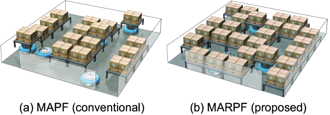
Figure 1: Environments of MAPF and MARPF. MAPF needs passages, whereas MARPF does not.

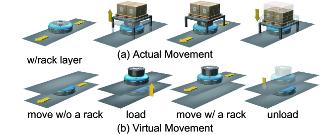
Figure 2: Two layers to express AGVs movements.

I-A Contribution

Original multi-agent pickup and delivery (MAPD) focuses only on conveying target racks, while some studies also consider exchanging the positions of racks [6, 7]. The difference between MARPF and rearrangement-considering MAPD is outlined as follows:

• MARPF: Only the target racks are assigned goals, and the obstacle racks are situated freely.

• Rearrangement-considering MAPD: All racks are assigned goals.

It could be posited that rearrangement-considering MAPD can potentially address MARPF by assigning the same goal positions as the initial positions for obstacle racks. However, we estimate two typical situations where this assumption may not apply: (1) Environments with highly dense racks, where some situations cannot be solved by rearrangement-considering MAPD (Fig. 3). Sufficient conditions for solvability are discussed in a sliding tile puzzle [8]; and (2) Environments with dense racks and a limited number of AGVs, where relocating racks to their initial positions would require a significant number of time steps. The optimization problem of where to relocate the obstacle racks is challenging, and MARPF constitutes a new problem.

The main contributions of this study are as follows:

• Define a new problem (MARPF) of planning paths for AGVs to convey target racks to their designated locations in dense environments.

• Propose a method for solving MARPF, a formulation as an ILP problem in a network flow.

• Propose an application of MARPF for real-time solving combined with cooperative A* (CA*).

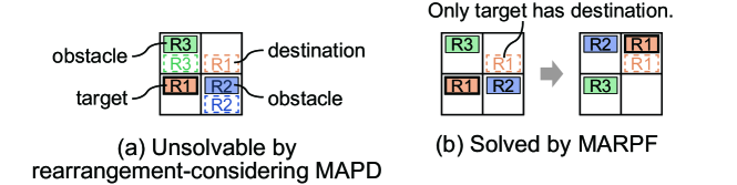
Figure 3: Unsolvable example by MAPD.

I-B Related Work

I-B1 MAPF

The MAPF problem concerns finding the optimal paths for multiple agents without collisions, and numerous methods have been proposed [1]. As complete and optimal solvers, there are conflict-based search (CBS) [9], improved CBS [10], and enhanced CBS [11]. Prioritized planning, such as CA* [12] and multi-label A* [13], has a short runtime but is suboptimal. MAPD [14] is a lifelong variant of MAPF. Specifically, in MAPD, each agent is constantly assigned new tasks with new goal locations, whereas in MAPF, each agent has only one task.

I-B2 Rearrangement-considering MAPD

In Double-Deck MAPD (DD-MAPD) [6], agents are tasked to move racks to their assigned delivery locations, thereby changing the overall arrangement of the racks. Their algorithm for DD-MAPD solves a DD-MAPD instance with $M$ agents and $N$ racks by decomposing it into an $N$-agent MAPF instance, followed by a subsequent $M$-agent MAPD instance with task dependencies. In Multi-Agent Transportation (MAT) [7], all racks are also assigned delivery locations without fixed aisles. They provides an algorithm for solving MAT by reducing it to a series of satisfiability problems.

II Problem Definition

In this section, we define the MARPF problem. As noted in Section I, MARPF aims to plan paths for AGVs to convey target racks in an environment without passages. Table I lists the notation used in the following sections.

TABLE I: Notations.

Symbols	Description
Section II and after
$a_{i}$	AGV $i$
$r_{i}$	Rack $i$
$x\in\{0,\cdots,size_{x}-1\}$	Column index ($size_{x}$ is the grid width)
$y\in\{0,\cdots,size_{y}-1\}$	Row index ($size_{y}$ is the grid height)
$v_{x,y}$	Vertex
$V$	Set of vertices
$E$	Set of edges
$G=(V,E)$	Connected undirected graph
$t$	Timestep
$loc^{t}(a_{i})$	Location vertex of $a_{i}$ at timestep $t$
$load^{t}(a_{i})$	Rack loading state of $a_{i}$ at timestep $t$
Section III and after
$G^{+}_{ag}=(V^{+}_{ag},E^{+}_{ag})$	Time-expanded network representing
	all AGVs’ movements
$G^{+}_{ar}=(V^{+}_{ar},E^{+}_{ar})$	Time-expanded network representing
	all racks’ movements
$G^{+}_{tr}=(V^{+}_{tr},E^{+}_{tr})$	Time-expanded network representing
	the target rack’s movements
$\mathcal{T}$	Set of timesteps in time-expanded
	networks
$c(\cdot)$	Cost function of flow
$l$	Layer (w/rack or w/o rack)
$S_{ag},S_{ar},S_{tr}\subseteq V$	Start location vertices of all AGVs, all
	racks, and the target racks respectively
$T_{tr}\subseteq V$	Goal location vertex of the target rack
$\alpha^{t}_{vi,vo,li,lo},\beta^{t}_{vi,vo},\gamma^{t}_{vi,vo}$	Flow on $E^{+}_{ag},E^{+}_{ar},E^{+}_{tr}$ respectively

An MARPF instance comprises $M$ AGVs, $N$ racks, and an undirected grid graph, $G=(V,E)$.

$$V=\{v_{x,y}\,|\,x\in\{0,\cdots,size_{x}-1\},y\in\{0,\cdots,size_{y}-1\}\}$$

$$E=\{(v_{x,y},v_{x^{\prime},y^{\prime}})\,|\,v_{x,y},v_{x^{\prime},y^{\prime}}\in V,|x-x^{\prime}|+|y-y^{\prime}|=1\},$$

where $v_{x,y}\in V$ is the vertex with the column index $x$ and the row index $y$ in the grid. $loc^{t}(a_{i}),loc^{t}(r_{i})\in V$ denote the vertices of AGV $a_{i}$ and rack $r_{i}$ at timestep $t$, respectively. $load^{t}(a_{i})\in\{0,1\}$ refers to the rack-loading state of AGV $a_{i}$ at timestep $t$, where $1$ represents loading, and $0$ represents unloading. At each time step $t$, an AGV executes one of the following actions: (1) Remain at the current location $loc^{t}(a_{i})=loc^{t+1}(a_{i})$; (2) Move to the next location $\left(loc^{t}(a_{i}),loc^{t+1}(a_{i})\right)\in E$; (3) Load a rack $load^{t}(a_{i})=0$, $load^{t+1}(a_{i})=1$, $loc^{t}(a_{i})=loc^{t+1}(a_{i})$; (4) Unload a rack $load^{t}(a_{i})=1$, $load^{t+1}(a_{i})=0$, $loc^{t}(a_{i})=loc^{t+1}(a_{i})$. A rack also executes one of the following actions: remain $loc^{t}(r_{i})=loc^{t+1}(r_{i})$ or move $\left(loc^{t}(r_{i}),loc^{t+1}(r_{i})\right)\in E$; however, its movement depends on AGVs because the rack does not move by itself.

There should be no collisions between agents or racks. We define three types of collision for agents (Fig. 4): First is the vertex conflict [1], where two agents cannot be in the same location at the same timestep. Second is the swapping conflict [1], where two agents cannot move along the same edge in opposite directions at the same timestep. Third is the corner conflict. Two adjacent agents cannot move vertically at the same timestep since their corners (or the corners of their conveying racks) collide. Formally, for all agents $a_{i},a_{j}\,(i\neq j)$ and all timesteps $t$, it must hold the following equations:

$$loc^{t}(a_{i})\neq loc^{t}(a_{j})$$ (1)

$$loc^{t}(a_{i})=loc^{t+1}(a_{j})$$

$$\Rightarrow\left(loc^{t+1}(a_{i})_{x}-loc^{t}(a_{i})_{x}\right)=\left(loc^{t+1}(a_{j})_{x}-loc^{t}(a_{j})_{x}\right)$$

$$\quad\wedge\left(loc^{t+1}(a_{i})_{y}-loc^{t}(a_{i})_{y}\right)=\left(loc^{t+1}(a_{j})_{y}-loc^{t}(a_{j})_{y}\right),$$ (2)

where $loc^{t}(a_{i})_{x}$ and $loc^{t}(a_{i})_{y}$ denote the column and row indices of $loc^{t}(a_{i})$, respectively. (1) represents the vertex conflict. (2) represents the both of the swapping conflict and the corner conflict. The above three types of collision are also applied to racks.

The MARPF problem involves computing collision-free paths for AGVs and minimizing the timesteps required to convey the target racks to their designated locations. Non-target racks act as obstacles and are positioned freely.

Fig. 5 exemplifies moving a rack to avoid interference with the movement of the target rack. The path the AGV must move to convey the target rack to its designated location is blocked by an obstacle rack (Fig. 5(a)). First, the obstacle rack is removed (Fig. 5(b)), and the target rack is then conveyed to the designated location (Fig. 5(c)).

III Proposed Method

In this section, we formulate MARPF as a minimum-cost flow problem in a network flow, similar to the approaches for MAPF [5, 15]. Two types of synchronized networks are established, one for AGVs and the other for racks. AGVs’ network distinguishes whether or not an AGV is loading a rack using two virtual layers to represent loading a rack.

III-A Definition of Networks

When AGVs are not conveying a rack, their obstacles are the other AGVs; however, when they are conveying a rack, other racks also become obstacles. Therefore, it must be determined whether an AGV is loading a rack onto a time-expanded network. The AGVs’ movements are classified into the following four actions in terms of the rack-loading state (Fig. 2(a)):

1. Move (or remain at the current location) without a rack.

2. Load a rack.

3. Move (or remain at the current location) with a rack.

4. Unload a rack.

The proposed method divides a moving plane into two virtual layers to represent two situations: loading or not loading a rack (Fig. 2(b)). The rack-loading action corresponds to movement from the w/o to the w/rack layers, and vice versa.

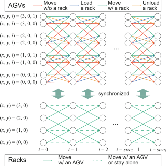
Figure 6: Time-expanded networks for AGVs (upper) and racks (lower).

Then, all vertices are expanded along the time-axis, and under specific constraints, directed edges are added. The edges indicate AGV motion in the grid. The motions are distinguished by the indices $(x,y)$ of the source and sink vertices and the virtual layers, where the motion is with ($l=1$) and without ($l=0$) a rack. Fig. 6 (upper) shows an example of a time-expanded network representing all AGVs’ movements. For simplicity, Figs. 2 and 6 show the moving plane in one dimension; however, it is two-dimensional.

For rack’s movements, the networks should be separated from the AGVs. Distinguishing the layers in a time-expanded network is not necessary (Fig. 6 (lower)). The flows expressing the movements of racks are synchronized with the corresponding flows of AGVs.

We define the time-expanded network representing all AGVs, all racks, and the target rack’s movements as directed graphs $G^{+}_{ag}=(V^{+}_{ag},E^{+}_{ag})$, $G^{+}_{ar}=(V^{+}_{ar},E^{+}_{ar})$, and $G^{+}_{tr}=(V^{+}_{tr},E^{+}_{tr})$, respectively. $G^{+}_{tr}$ has the same structure as $G^{+}_{ar}$; however, the target rack is distinguished from the other racks.

$$\begin{array}[]{@{}l@{}l@{}}V^{+}_{ag}=\{v^{t}_{x,y,l}\,|&\,x\in\{0,\cdots,size_{x}-1\},y\in\{0,\cdots,size_{y}-1\},\\ &l\in\{0,1\},t\in\{0,\cdots,size_{t}\}\}\end{array}$$

$$\begin{array}[]{@{}l@{}l@{}}E^{+}_{ag}=\{\langle v^{t}_{x,y,l},v^{t^{\prime}}_{x^{\prime},y^{\prime},l^{\prime}}\rangle\,|&\,v^{t}_{x,y,l},v^{t^{\prime}}_{x^{\prime},y^{\prime},l^{\prime}}\in V^{+}_{ag},\\ &|x-x^{\prime}|+|y-y^{\prime}|\leq 1,t^{\prime}-t=1\}\end{array}$$

$$\begin{array}[]{@{}l@{}l@{}}V^{+}_{ar},V^{+}_{tr}=\{v^{t}_{x,y}\,|&\,x\in\{0,\cdots,size_{x}-1\},\\ &y\in\{0,\cdots,size_{y}-1\},t\in\{0,\cdots,size_{t}\}\}\end{array}$$

$$\begin{array}[]{@{}l@{}l@{}}E^{+}_{ar},E^{+}_{tr}=\{\langle v^{t}_{x,y},v^{t^{\prime}}_{x^{\prime},y^{\prime}}\rangle\,|&\,v^{t}_{x,y},v^{t^{\prime}}_{x^{\prime},y^{\prime}}\in V^{+}_{ar},\\ &|x-x^{\prime}|+|y-y^{\prime}|\leq 1,t^{\prime}-t=1\},\end{array}$$

where $size_{t}$ denotes the maximum of timesteps in the time-expanded network. Dependencies exist between $G^{+}_{ar}$ and $G^{+}_{ag}$ and between $G^{+}_{tr}$ and $G^{+}_{ar}$, and their flows are synchronized.

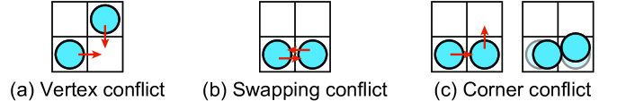
Figure 4: Type of conflicts.

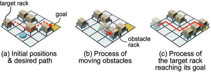
Figure 5: Problem example.

III-B Definition of Variables

The vertices on $V^{+}_{ag}$ are distinguished by $t,v$, and $l$. $\alpha^{t}_{vi,vo,li,lo}$ represents the flow on the edge $\langle v^{t}_{vi_{x},vi_{y},li},v^{t+1}_{vo_{x},vo_{y},lo}\rangle\in E^{+}_{ag}$, where $vi,vo\in V,li,lo\in\{0,1\}$ respectively denote the source vertex, sink vertex, source layer, and sink layer while $t\in\mathcal{T}=\{0,\cdots,size_{t}-1\}$ represents the source vertex’s timestep. $G^{+}_{ar},G^{+}_{tr}$ do not contain multiple layers; therefore, the flows of racks are expressed more simply as $\beta^{t}_{vi,vo},\gamma^{t}_{vi,vo}$, respectively. We define the variables and the cost function $c(\cdot)$ as follows:

$$\alpha^{t}_{vi,vo,li,lo},\beta^{t}_{vi,vo},\gamma^{t}_{vi,vo}\in\{0,1\}$$ (3)

$$c(vi,vo,li,lo,t)=\left\{\begin{array}[]{ll}0&\text{if }\,vi=vo,li=lo\\ t+1&\text{otherwise}\end{array}\right.$$ (6)

We define the initial location vertices of all AGVs, racks, and the target rack respectively as $S_{ag},S_{ar}$, and $S_{tr}$, where $S_{tr}\subseteq S_{ar}$. In the network, we express the initial locations by fixing the flows at $t=0$ (respectively (9), (12), and (15)). The goal location vertex of the target rack, $T_{tr}$, is defined by (18).

$$\left\{\begin{array}[]{ll}\alpha^{0}_{vi,vo,li,lo}=1&\text{if }\,vi=vo\in S_{ag},li=lo=0\\ \alpha^{0}_{vi,vo,li,lo}=0&\text{otherwise}\end{array}\right.$$ (9)

$$\left\{\begin{array}[]{ll}\beta^{0}_{vi,vo}=1&\text{if }\,vi=vo\in S_{ar}\\ \beta^{0}_{vi,vo}=0&\text{otherwise}\end{array}\right.$$ (12)

$$\left\{\begin{array}[]{ll}\gamma^{0}_{vi,vo}=1&\text{if }\,vi=vo\in S_{tr}\\ \gamma^{0}_{vi,vo}=0&\text{otherwise}\end{array}\right.$$ (15)

$$\left\{\begin{array}[]{ll}\gamma^{size_{t}-1}_{vi,vo}=1&\text{if }\,vi=vo\in T_{tr}\\ \gamma^{size_{t}-1}_{vi,vo}=0&\text{otherwise}\end{array}\right.$$ (18)

III-C Minimum Cost Flow Problem

The purpose is to convey the target rack from the starting position to the goal position as quickly as possible. The set of timesteps $\mathcal{T}\setminus\{size_{t}-1\}$ refers to $\mathcal{T}^{-}$.

$$\text{min}\,\sum c(vi,vo,li,lo,t)\alpha^{t}_{vi,vo,li,lo}$$ (19)

s.t.

$$\sum_{vi,li}\alpha^{t}_{vi,v,li,l}=\sum_{vo,lo}\alpha^{t+1}_{v,vo,l,lo} \forall v\in V,l\in\{0,1\},t\in\mathcal{T}^{-}$$ (20)

$$\sum_{vi}\beta^{t}_{vi,v}=\sum_{vo}\beta^{t+1}_{v,vo} \forall v\in V,t\in\mathcal{T}^{-}$$ (21)

$$\sum_{vi}\gamma^{t}_{vi,v}=\sum_{vo}\gamma^{t+1}_{v,vo} \forall v\in V,t\in\mathcal{T}^{-}$$ (22)

$$\beta^{t}_{vi,vo}=\alpha^{t}_{vi,vo,1,1} \forall(vi,vo)\in E,t\in\mathcal{T}$$ (23)

$$\gamma^{t}_{vi,vo}\leq\beta^{t}_{vi,vo} \forall vi,vo\in V,t\in\mathcal{T}$$ (24)

$$\alpha^{t}_{v,v,0,1}\leq\sum_{vi}\beta^{t}_{vi,v} \forall v\in V,t\in\mathcal{T}$$ (25)

$$\sum_{vi,li,lo}\alpha^{t}_{vi,v,li,lo}\leq 1\, \forall v\in V,t\in\mathcal{T}$$ (26)

$$\sum_{vi}\beta^{t}_{vi,v}\leq 1 \forall v\in V,t\in\mathcal{T}$$ (27)

$$\sum_{li,lo}\alpha^{t}_{vi,vo,li,lo}+\sum_{v,li,lo}\alpha^{t}_{vo,v,li,lo}$$

$$\leq\sum_{\hat{v}_{2x^{\prime}-x,2y^{\prime}-y},li,lo}\alpha^{t}_{vo,\hat{v},li,lo}+1 \forall(vi_{x,y},vo_{x^{\prime},y^{\prime}})\in E,t\in\mathcal{T}$$ (28)

The objective function (19) defines the cost function, which implies that the larger the timestep $t$, the higher the movement cost. Therefore, this problem calculates the flows with the minimum number of steps to convey the target rack from the initial to the goal position.

Constraints (20)–(22) are required to satisfy the flow conservation constraints at the vertices. Racks are conveyed by AGVs, and (23) indicates that the flows of the racks’ movements on $G^{+}_{ar}$ are equal to the corresponding flow on $G^{+}_{ag}$. Constraint (23) indicates that $G^{+}_{ar}$ depends on $G^{+}_{ag}$ and (24) indicates that $G^{+}_{tr}$ depends on $G^{+}_{ar}$. Considering (15), (22), and (24), only flows related to the movement of the target rack on $G^{+}_{ar}$ are reflected in $G^{+}_{tr}$. Constraint (25) indicates that a rack must exist where an AGV loads a rack ($\alpha^{t}_{v,v,0,1}=1$). Eq. $\sum_{vi}\beta^{t}_{vi,v}=1$ indicates that one of the flows to vertex $v$ is $1$; that is, a rack is placed at vertex $v$. Constraints (26) and (27) prohibit AGVs and racks from coexisting at the same vertices, respectively. Constraint (28) is required to prevent the swapping conflict and the corner conflict between agents.

The above formulation is for one target rack. However, the formulation can be extended to multiple target racks. The network representing the movement of the $i$-th target rack is referred to as $G^{+,i}_{tr}=(V^{+,i}_{tr},E^{+,i}_{tr})$. The corresponding flow is $\gamma^{t,i}_{vi,vo}$ and the constraints are the same as $\gamma^{t}_{vi,vo}$.

III-D Applications for Real-Time Solving

The proposed method complicates the network with longer path lengths and the computational cost increases exponentially. We believe that appropriately dividing the path reduces the computational costs. Hence, we propose an acceleration method combined with CA*, called CA*-ILP. This method comprises global and local searches.

First, path finding is performed using CA* for the global search. In this step, the racks are assumed to move by themselves, and collisions between racks are allowed. However, from the viewpoint of timesteps, removing obstacle racks should be avoided. Therefore, moving to a location with a rack is defined as incurring a $\kappa>1$ cost in CA*. Moving to a location with no racks incurs a cost of $+1$. Algorithm 1 presents the corresponding pseudo-code. The global search executes CA* [line 1]. It chooses the waypoints according to the global paths [lines 2–7]. Paths may be indivisible by the span length $\tau$ between waypoints, and fractions are rounded [line 8].

Second, the local search repeatedly solves the local path-finding problem. The local path-finding problem of conveying multiple racks to their waypoints is solved using ILP. Multiple racks do not always arrive at their waypoint simultaneously. When one of the rack arrives at its waypoint, a local search is performed again.

Algorithm 1 Global Search

Input: Initial location $n^{i}_{0}$ and the goal location $n^{i}_{g}$ of the $i$-th target rack
Parameter: Span length $\tau$ between two waypoints
Output: Sequences of waypoints $waypoint^{i}$

1:Find the global paths of the target racks using CA*: $path^{i}=(n^{i}_{0},n^{i}_{1},\cdots,n^{i}_{g})$, which is a vertex sequence.

2:for all $i$ do

3:    $waypoint^{i}=()$

4:    for all $p<|path^{i}|$ do

5:        $p=\tau q+r\,(0\leq r<q)$

6:        if $r=0$ and $\tau(q+1)\leq|path^{i}|$ then

7:           $waypoint^{i}\leftarrow$ add $n^{i}_{p}$             

8:    $waypoint^{i}\leftarrow$ add $n^{i}_{g}$

IV Experiments

In this section, we describe two experiments: (1) a comparative evaluation of the proposed method against existing methods; and (2) an evaluation of the effectiveness of CA*-ILP. For the experimental setup, the time-expanded networks are represented by NetworkX and the optimization problem is defined by PuLP. We use the GUROBI solver. All the experiments were run on a system comprising Ubuntu 22.04, Intel Core i9-12900K, and 128 GiB of RAM.

We performed all the experiments in $6\times 4$ grids. Although this size is too small for automated warehouses, small-sized environments, such as inter-process transportation, are utilized in specific areas of the factories.

IV-A Experiment 1: Comparative Evaluation of the Proposed Method against Existing Methods

We compared our proposed method against widely used MAPF solvers CA* and CBS. In MARPF, the other racks become obstacles only when the AGV conveys a rack. We used CA* and CBS for comparison, which accounts for these conditions.

The first step had two AGVs and six racks, including targets; the racks were then added sequentially. Fig. 7(a) illustrates this environment. Two obstacle racks could block the paths. For example, two racks were placed in the lower-left region (Fig. 7(b)). We performed 30 experiments at different locations to add the racks. The solver’s time limit was 120 s.

Fig. 8 compares the success rates and average makespans of the successful tasks. As Fig. 8 shows, with few added racks, all methods succeeded. However, with many added racks, CA* and CBS sometimes failed to find the path. CA* and CBS consider only the movements of the target racks and cannot remove obstacle racks. Therefore, they cannot find the path when many racks are added and the paths are blocked. Our proposed method considers all rack movements such that the movement for removing obstacle racks is found.

The proposed method is theoretically capable of solving these problems if there are one or more empty vertices. However, it fails in half of the tasks when adding six racks. When the problem is complex, and the computational cost is high, the solver fails to find a path within the time limit. Therefore, the following experiment evaluated an acceleration method.

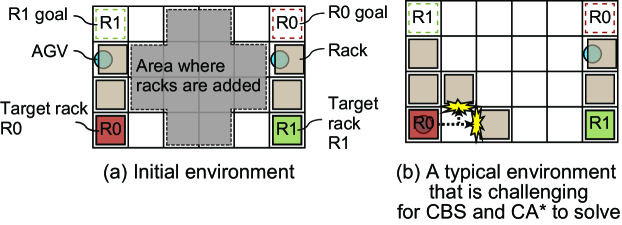
Figure 7: Environment of Exp. 1.

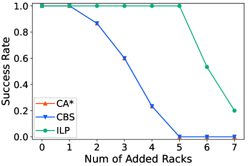
Figure 8: Comparison of success rates on Exp. 1.

IV-B Experiment 2: Evaluation of the Effectiveness of CA*-ILP

Solving the path-finding problem using the proposed method is computationally expensive. We confirm that CA*-ILP reduces the computational cost. We assigned a cost $\kappa=3$ to move to a location occupied by a rack.

The evaluations were conducted in sparse (12 racks) and dense (18 racks) environments. Each environment contained eight AGVs. Fig. 9 illustrates an example of a dense environment. We performed 30 experiments with the AGVs and non-target racks in different initial locations to compare the makespans of the tasks of conveying the two target racks to their goals. Table II compares the makespans, highlighting the differences in span lengths between waypoints (CA*-ILP). Fig. 10 also compares the makespans between the initially proposed method (ILP-only) and the acceleration method (CA*-ILP). We set the time limit of 120 s for each local search conducted by CA*-ILP. ILP-only is computationally expensive; therefore, we set the time limit to three different values, 120, 240, and 1200 s, and compared them. In the dense environment (Fig. 10(b)), ILP-only failed to find solutions in some experiments within the time limits of 120 and 240 s.

First, we evaluated the difference in span between waypoints (CA*-ILP). According to Table II, span 4 yielded the best result. Span 1, being excessively fine-grained and ignoring future rack locations, had a larger makespan. We adopted spans 2 and 4 for the subsequent comparisons.

Second, we compared the initially proposed method (ILP-only) with the acceleration method (CA*-ILP). In the sparse environment (Fig. 10(a)), CA*-ILP exhibited a shorter total calculation time compared with ILP-only; however, its makespan was larger. CA*-ILP divides the paths into several parts, each easier to solve, thereby reducing the overall calculation cost compared to ILP-only. However, because the waypoints in CA*-ILP are not always optimal, its makespan exceeded that of the global optimal solution by ILP-only.

In the dense environment (Fig. 10(b)), the makespan of CA*-ILP was smaller than ILP-only, and the total calculation time of CA*-ILP was considerably shorter than ILP-only. In the dense environment, the computation cost was higher than in the sparse environment, and CA*-ILP was more effective in calculating time. In all experiments ILP-only found the feasible solution within the time limit of 1200 s; however, ILP-only does not always find the good feasible solution within the time limit. As a result, the average makespan of CA*-ILP was smaller than ILP-only.

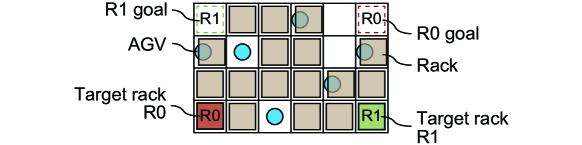
Figure 9: Example of the environment in Exp. 2.

TABLE II: Comparison of CA*-ILP makespans on Exp. 2.

Span length $\tau$ between waypoints	1	2	4
12 racks	21.9	18.1	14.8
20 racks	39.9	28.9	23.9

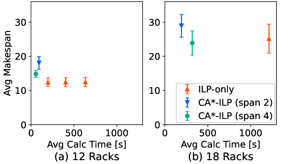
Figure 10: Comparison of makespans on Exp. 2.

V Conclusion

In this study, we defined the MARPF problem for planning the paths of target racks to their designated locations using AGVs in dense environments without passages. We developed an ILP-based formulation for synchronized time-expanded networks by dividing the movements of AGVs and racks. The proposed method optimized the paths to move the obstacles and convey the target racks. By recognizing the complexity that increases with path length, we also presented an acceleration method combined with CA*. Our experiments confirmed that the acceleration method reduced computational cost. While we acknowledge the need for further research into more efficient algorithms, it is sufficient if the paths are calculated before the following product is completed in conveyance between production processes in factories. In these instances, our proposed algorithm can be practically applied.

Although we performed our experiments on a small grid, the problem setting of MARPF can be applied to large-scale warehouses. However, solving large problems increases the computational cost. In the future, we plan to investigate more efficient and faster algorithms.

References

- [1] R. Stern, N. Sturtevant, A. Felner, S. Koenig, H. Ma, T. Walker, J. Li, D. Atzmon, L. Cohen, T. K. Kumar, R. Barták, and E. Boyarski, “Multi-Agent Pathfinding: Definitions, Variants, and Benchmarks,” in Proceedings of the International Symposium on Combinatorial Search, vol. 10, 2019, pp. 151–158.
- [2] P. R. Wurman, R. D’Andrea, and M. Mountz, “Coordinating Hundreds of Cooperative, Autonomous Vehicles in Warehouses.” AI Magazine, vol. 29, no. 1, pp. 9–20, 2008.
- [3] W. Honig, S. Kiesel, A. Tinka, J. W. Durham, and N. Ayanian, “Persistent and Robust Execution of MAPF Schedules in Warehouses,” IEEE Robotics and Automation Letters, vol. 4, no. 2, pp. 1125–1131, 2019.
- [4] J. Li, H. Zhang, M. Gong, Z. Liang, W. Liu, Z. Tong, L. Yi, R. Morris, C. Pasareanu, and S. Koenig, “Scheduling and Airport Taxiway Path Planning Under Uncertainty,” in Proceedings of the 2019 Aviation and Aeronautics Forum and Exposition, 2019, pp. 1–8.
- [5] A. Okoso, K. Otaki, S. Koide, and T. Nishi, “High Density Automated Valet Parking via Multi-agent Path Finding,” in 2022 IEEE 25th International Conference on Intelligent Transportation Systems (ITSC), 2022, pp. 2146–2153.
- [6] B. Li and H. Ma, “Double-Deck Multi-Agent Pickup and Delivery: Multi-Robot Rearrangement in Large-Scale Warehouses,” IEEE Robotics and Automation Letters, pp. 1–8, 2023.
- [7] P. Bachor, R.-D. Bergdoll, and B. Nebel, “The Multi-Agent Transportation Problem,” in Proceedings of the AAAI Conference on Artificial Intelligence, vol. 37, 2023, pp. 11 525–11 532.
- [8] W. W. Johnson and W. E. Story, “Notes on the “15” Puzzle,” American Journal of Mathematics, vol. 2, no. 4, pp. 397–404, 1879.
- [9] G. Sharon, R. Stern, A. Felner, and N. R. Sturtevant, “Conflict-based search for optimal multi-agent pathfinding,” Artificial Intelligence, vol. 219, pp. 40–66, 2015.
- [10] E. Boyarski, A. Felner, R. Stern, G. Sharon, O. Betzalel, D. Tolpin, and E. Shimony, “ICBS: The Improved Conflict-Based Search Algorithm for Multi-Agent Pathfinding,” in Proceedings of the International Symposium on Combinatorial Search, vol. 6, 2015, pp. 223–225.
- [11] M. Barer, G. Sharon, R. Stern, and A. Felner, “Suboptimal Variants of the Conflict-Based Search Algorithm for the Multi-Agent Pathfinding Problem,” in Proceedings of the International Symposium on Combinatorial Search, vol. 5, 2014, pp. 19–27.
- [12] D. Silver, “Cooperative Pathfinding,” in Proceedings of the AAAI Conference on Artificial Intelligence and Interactive Digital Entertainment, vol. 1, 2005, pp. 117–122.
- [13] F. Grenouilleau, W.-J. van Hoeve, and J. N. Hooker, “A Multi-Label A* Algorithm for Multi-Agent Pathfinding,” in Proceedings of the International Conference on Automated Planning and Scheduling, vol. 29, 2021, pp. 181–185.
- [14] H. Ma, J. Li, T. K. S. Kumar, and S. Koenig, “Lifelong Multi-Agent Path Finding for Online Pickup and Delivery Tasks,” in Proceedings of the International Joint Conference on Autonomous Agents and Multiagent Systems, 2017, pp. 837–845.
- [15] J. Yu and S. M. LaValle, “Planning Optimal Paths for Multiple Robots on Graphs,” in 2013 IEEE International Conference on Robotics and Automation, 2013, pp. 3612–3617.