Semisupervised score based matching algorithm to evaluate the effect of public health interventions

Abstract

Multivariate matching algorithms ”pair” similar study units in an observational study to remove potential bias and confounding effects caused by the absence of randomizations. In one-to-one multivariate matching algorithms, a large number of ”pairs” to be matched could mean both the information from a large sample and a large number of tasks, and therefore, to best match the pairs, such a matching algorithm with efficiency and comparatively limited auxiliary matching knowledge provided through a ”training” set of paired units by domain experts, is practically intriguing.

We proposed a novel one-to-one matching algorithm based on a quadratic score function $S_{\beta}(x_{i},x_{j})=\beta^{T}(x_{i}-x_{j})(x_{i}-x_{j})^{T}\beta$. The weights $\beta$, which can be interpreted as a variable importance measure, are designed to minimize the score difference between paired training units while maximizing the score difference between unpaired training units. Further, in the typical but intricate case where the training set is much smaller than the unpaired set, we propose a semisupervised companion one-to-one matching algorithm (SCOTOMA) that makes the best use of the unpaired units. The proposed weight estimator is proved to be consistent when the truth matching criterion is indeed the quadratic score function. When the model assumptions are violated, we demonstrate that the proposed algorithm still outperforms some popular competing matching algorithms through a series of simulations. We applied the proposed algorithm to a real-world study to investigate the effect of in-person schooling on community Covid-19 transmission rate for policy making purpose.

, and

1 Introduction

In the past year, roaring COVID-19 cases across the country, consisting mainly of the omicron variant, has aroused much controversy regarding in-person education for children and adolescents. Reopening schools would inevitably increases social interactions and contributes to the disease’s community transmission, causing the policymakers to make painful trade-off between teaching quality and COVID-19 virus prevention. Naturally, an observational study that quantifies the increment in transmission rate due to school reopening would help design related policies. However, such a study would be subject to confounders caused by vastly different community factors. As a potential solution, matching algorithms select a subset of comparable observations in each treatment group and balance the distributions of (possibly confounded) baseline covariates, and therefore, remove the bias in the estimated treatment effect. Most ideally, in the school reopening policy evaluation problem with two treatments namely reopening and closed, a reopened county should match to some closed counties with the same community factors; but such exact matching is infeasible when the community factors to be matched are more than just a few and are sparsely distributed. The best we can do is pairing each reopened county to a distinguished closed county with most ”similar” integrated baseline factors’ impacts, i.e., a one-to-one matching algorithm that throughly utilize the information in a sparsely distributed dataset.

Intuitively, one can seamlessly pair a reopened county with the ”closest” controlled county, i.e., closed county, with a distance measure or a score function that describes how different two observations are regarding their covariates. Popular distance measures include Euclidean distance and Mahalanobis distance. For $N$ controlled, closed counties, and $M$ treated, reopened counties, each with $p$ individual baseline characteristics stored separately in $(\tilde{X}_{c})_{N\times p}$, $(\tilde{X}_{t})_{M\times p}$, denote their $i^{th}$ and $j^{th}$ observations as $\tilde{x}_{c,i}^{T}=(\tilde{X}_{c})_{i}=(\tilde{x}_{c,i1},\cdots,\tilde{x}_{c,ip})$ and $\tilde{x}_{t,j}^{T}=(\tilde{X}_{t})_{j}=(\tilde{x}_{t,j1},\cdots,\tilde{x}_{t,jp})$ respectively. Then their Euclidean Distance and Mahalanobis Distance are

$$(\tilde{x}_{c,i}-\tilde{x}_{t,j})^{T}(\tilde{x}_{c,i}-\tilde{x}_{t,j})\;\;and\;\;(\tilde{x}_{c,i}-\tilde{x}_{t,j})^{T}S^{-1}(\tilde{x}_{c,i}-\tilde{x}_{t,j}),$$ (1.1)

where $S$ is the sample covariance matrix. On the contrary, the propensity score proposed by Rosenbaum and Rubin (1983) is a substitution for the distance function who focus on the integrated impact of each observation’s covariates. One can control solely the propensity score to balance the overall distributions of all covariates in the control and treatment groups. Assuming treatment assignments are independent, the propensity score for $i^{th}$ observation $\tilde{x}_{i}$ can be written as

$$p(\tilde{x}_{i})=P(i^{th}{\rm\ district\ is\ reopened}|X=\tilde{x}_{i}).$$ (1.2)

It is also proposed in Rosenbaum and Rubin (1985) to use a logit transformation of each $p(\tilde{x}_{i})$ as the results oftentimes behave like a normal distribution, and estimate $p(\tilde{x}_{i})$ using logistic regression algorithms or similar classification algorithms since the propensity score is essentially a conditional probability of treatment assignment. We refer more variants of the propensity score matching methods to Stuart (2010) and the references within.

However, existing distance measures used by matching algorithms usually weigh all baseline covariates the same or weigh them simply by analogs of their variances. Although this might be the optimal solution in some circumstances, it is not the case for one-to-one matching problems with large $p$. Contemporary observational studies suffer from the computational complexity brought by a vast number of covariates, e.g., the aforementioned distance measures would fail as similarity measures in Giraud (2021) where all observations are dictated to be at a similar distance from the others. Likewise, the propensity score matching is merely exercisable but in a different manner in the school reopening policy evaluation problem. It suffers from the matching exclusiveness of one-to-one matching and the sparsely distributed community factors because the propensity score matching usually requires large samples with substantial overlap between treatment and control groups to estimate an average treatment effect and to overcome the large $p$. There are many attempts to alleviate these problems by performing dimension reduction (Peng, Ngo and Xiao, 2007) or transformation techniques (Han et al., 2007) on the training observations before measuring their similarities. Nevertheless, these approaches typically overweigh the variables that best explain the observations, which do not always coincide with the variables most influential to the matching. Instead, an ideal dimension reduction or transformation technique should extract each baseline covariates’ impact to pairing while maximizing information utilization within the paired observations.

To compensate for aforementioned matching algorithms’ inadequateness, we use a semisupervised dataset consists of training and object observations, where the training observations are reviewed by experts in infectious disease and health disparities, biologists, and policy makes, etc., with a small portion of the observations been paired because the time required for manually matching all observations are commonly prohibitive. Accordingly, two popular, different but closely related approaches to invoke side information like the supervised knowledge is distance metric learning (DML) and Fisher’s linear discriminant analysis (LDA). DML has been studied and made an prominent contribution in the field of image retrieval (Hoi et al. (2006); Si et al. (2006); Weinberger and Saul (2009), etc.) and picture recognition (Bilenko, Basu and Mooney (2004); Globerson and Roweis (2005)). For instance, for a clustering problem with fully supervised training observations $\tilde{X}=\{\tilde{x}_{1},\cdots,\tilde{x}_{N}\}\subset\mathcal{M}_{p\times 1}$, define

$$\mathcal{S}=\big{\{}(\tilde{x}_{i},\tilde{x}_{j})\;|\;\tilde{x}_{i},\tilde{x}_{j}\in\tilde{X},\tilde{x}_{i}{\rm\;is\;in\;the\;same\;cluster\;with\;}\tilde{x}_{j}\big{\}},$$

$${\rm and\;\;} \mathcal{D}=\big{\{}(\tilde{x}_{i},\tilde{x}_{j})\;|\;\tilde{x}_{i},\tilde{x}_{j}\in\tilde{X},\tilde{x}_{i}{\rm\;is\;not\;in\;the\;same\;cluster\;with\;}\tilde{x}_{j}\big{\}},$$

Xing et al. (2002) propose to approximate the distance between two observations by

$$\big{(}d_{A}(\tilde{x}_{i},\tilde{x}_{j})\big{)}^{2}=(\tilde{x}_{i}-\tilde{x}_{j})^{T}A(\tilde{x}_{i}-\tilde{x}_{j})$$ (1.3)

with some positive semi-definite matrix $A$, and learn the metric $d_{A}$ by investigate the objective function

$$\min_{A\succeq 0}\sum_{(\tilde{x}_{i},\tilde{x}_{j})\in\mathcal{S}}d_{A}(\tilde{x}_{i},\tilde{x}_{j}),\quad s.t.,\;\;\sum_{(\tilde{x}_{i},\tilde{x}_{j})\in\mathcal{D}}d_{A}(\tilde{x}_{i},\tilde{x}_{j})\geq 1,$$ (1.4)

which generally needs to be solved by gradient descent and iterative projection algorithms (Rockafellar, 2015). This objective function (1.4) encourages $A$ to place within cluster observations close to each other while the constrain makes sure $A$ does not collapse all observations into a degenerated space, i.e., keeping different clusters’ observations away at a certain level. However, as pointed out in Si et al. (2006), the matrix $A$ learnt by (1.4) is not robust when training data $\tilde{X}$ is noisy or $N$ is small, instead, they add a penalty term to the objective function to regulate the size of the matrix $A$,

$$\min_{A\succeq 0}\;\;\bigg{[}\lVert A\rVert_{F}+C_{S}\sum_{(\tilde{x}_{i},\tilde{x}_{j})\in\mathcal{S}}d_{A}(\tilde{x}_{i},\tilde{x}_{j})-C_{D}\sum_{(\tilde{x}_{i},\tilde{x}_{j})\in\mathcal{D}}d_{A}(\tilde{x}_{i},\tilde{x}_{j})\bigg{]}.$$ (1.5)

Similar ideas also appeared in Hoi, Liu and Chang (2010) where they replaced the penalty of (1.5) by a Laplacian regularizer that is computed on solely the matrix $A$ and $\tilde{X}$ but not the pairing information $\mathcal{S}$ and $\mathcal{D}$. Other efforts such as Globerson and Roweis (2005), whom, for each $\tilde{x}_{i}$, define a conditional distribution over points $\tilde{x}_{j}|\tilde{x}_{i}$, $j\neq i$ as

$$\mathbb{P}_{A}(\tilde{x}_{j}|\tilde{x}_{i})=\frac{\exp\big{(}-d_{A}(\tilde{x}_{i},\tilde{x}_{j})\big{)}}{\sum_{k\neq i}\exp\big{(}-d_{A}(\tilde{x}_{i},\tilde{x}_{k})\big{)}}\cdot\mathbbm{1}(i\neq j),$$ (1.6)

and compare it with the oracle pairing information

$$\mathbb{P}_{0}(\tilde{x}_{j}|\tilde{x}_{i})=\mathbbm{1}(\tilde{x}_{j}\;{\rm is\;paired\;with\;}\tilde{x}_{i}),$$

accordingly, the distance metric is learnt by minimize the KL divergence

$$\min_{A\succeq 0}\sum_{i,j}KL\big{[}\mathbb{P}_{0}(\tilde{x}_{j}|\tilde{x}_{i})|\mathbb{P}_{A}(\tilde{x}_{j}|\tilde{x}_{i})\big{]}.$$ (1.7)

Meanwhile, LDA can be traced back to Fisher (1936) and had a great development by a series of works in the end of last century (Hastie, Tibshirani and Buja (1994), Hastie, Buja and Tibshirani (1995), Hastie and Tibshirani (1995), Hastie and Tibshirani (1996), etc.). Generally, for observations $\tilde{X}$ and supervision information $\mathcal{S}$ and $\mathcal{D}$, define the within cluster variance and the between cluster variance as

$$\Sigma_{w}=\frac{1}{N}\sum_{(\tilde{x}_{i},\tilde{x}_{j})\in\mathcal{S}}\frac{(\tilde{x}_{i}-\tilde{x}_{j})^{T}(\tilde{x}_{i}-\tilde{x}_{j})}{1+\sum_{k\neq i}^{1\leq k\leq N}\mathbbm{1}((\tilde{x}_{i},\tilde{x}_{k})\in\mathcal{S})},\;\;{\rm and}\;\;\Sigma_{b}=\frac{1}{N}\sum_{i=1}^{N}\tilde{x}_{i}^{T}\tilde{x}_{i}-\Sigma_{w},$$ (1.8)

respectively, then the distance metric $d_{A}$ defined in (1.3) can be learnt by maximize

$$\arg\max_{C\in\mathcal{M}_{k\times p}}\frac{\det\big{(}C\Sigma_{b}C^{T}\big{)}}{\det\big{(}C\Sigma_{w}C^{T}\big{)}},\quad{\rm and}\;\;A=C^{T}C,$$ (1.9)

where for an unlabeled data point $x$, the predicted $k$ dimensional label would be $Y=Cx$. For more details of LDA’s recent developments and its applications to image retrieval and recognition, we refer to Xing et al. (2002), Bar-Hillel et al. (2005), Hoi et al. (2006) and the references within.

Whereas, unlike image retrieval, matching accuracy is not the sole property we ask from the algorithm. For instance, because the similarities are measured in a transformed feature space, DML algorithms lack the interpretability of the matching results, which is desired in evaluating the treatment (county reopening) effect of public health intervention; While the classical LDA lacks the estimation efficiency because the within/between cluster variance $\Sigma_{w}$, $\Sigma_{b}$ defined in (1.8) can not address the similarity and the dissimilarity constraints properly for an one-to-one matching problem between the treatment and control group.

In this paper, we propose a semisupervised companion one-to-one matching algorithm (SCOTOMA) to pair each reopened county to a distinguished closed county. SCOTOMA directly seeks for an intuitive quadratic score function $S_{\beta}(x_{i},x_{j})=\beta^{T}(x_{i}-x_{j})(x_{i}-x_{j})^{T}\beta$ measuring the score difference between two observations, for which the weight $\beta$ can be seen as a variable importance measure for each baseline characteristics. It absorb ideas from different approaches and is build with a specialized similarity constraint and dissimilarity constraint like the construction in DML, a objective function analogous to LDA, and a penalty (regularization) term, to retain model interpretability and efficiency, and accommodate the large dimension $p$ simultaneously. Reopened counties are then paired with closed counties regard of their score differences with a tuning threshold. Further, for the case when the ratio of matched pairs and unmatched pairs are extremely small, we exploit the information in object observations set to build a self-taught learning framework.

The remainder of the paper is organized as follows. The proposed SCOTOMA and its properties are explained in detail in section 2. Simulations are presented in section 3 to evaluate SCOTOMA’s matching performance and compare it with other existing methods, while its application to a county reopening dataset during Covid-19 are carried out in section 4. A miscellany discussions are left to section 5.

2 Semisupervised companion one-to-one matching algorithm

Consider a semisupervised data set consists of training set $X$ and object set $\tilde{X}$. For the training set, we have $X^{T}=(\dot{X}^{T},\ddot{X}^{T})=(\dot{X}_{c}^{T},\dot{X}_{t}^{T},\ddot{X}_{c}^{T},\ddot{X}_{t}^{T})$, with $\dot{x}_{\iota,i}=(\dot{X}_{\iota})_{i}^{T}$ (and $\ddot{x}_{\iota,i}=(\ddot{X}_{\iota})_{i}^{T}$) being the transport of the $i$-th row (i.e., representing the $i$-th observation) of $\dot{X}_{\iota}$ (and $\ddot{X}_{\iota}$), $\iota\in\{c,t\}$; Here, $\dot{X}_{c},\dot{X}_{t}\in\mathcal{M}_{\dot{\ell}\times p}$ are $\dot{\ell}$ pairs of control and treatment observations in the training set matched by the experts with $(\dot{x}_{c,i},\dot{x}_{t,i})\in\mathcal{S}_{0}$, where

$$\mathcal{S}_{0}=\Big{\{}(\dot{x}_{c,z_{1}},\dot{x}_{t,z_{2}}):1\leq z_{1},z_{2}\leq\dot{\ell},\dot{x}_{c,z_{1}}\;{\rm is\;paired\;with\;}\dot{x}_{t,z_{2}}\Big{\}}=\Big{\{}(\dot{x}_{c,i},\dot{x}_{t,i})\Big{\}}_{1\leq i\leq\dot{\ell}};$$

Besides, we have $\ddot{X}_{c}\in\mathcal{M}_{\ddot{\ell}_{c}\times p}$ (and $\ddot{X}_{t}\in\mathcal{M}_{\ddot{\ell}_{t}\times p}$) being the unpaired observations in the control group (and treatment group) of the training set. Similarly, for the object set, we have $\tilde{X}=(\tilde{X}_{c}^{T},\tilde{X}_{t}^{T})^{T}\in\mathcal{M}_{(\tilde{\ell}_{c}+\tilde{\ell}_{t})\times p}$ with parallelly defined $\tilde{x}_{\iota,i}$, $\iota\in\{c,t\}$. When there is no confusion, we abuse the use of the notation, to denote $X$ (without loss of generality, we treat $\tilde{X}$, $\dot{X}$, $\dot{X}_{c}$, $\cdots$, in the same manner) as both the matrix and the observations set, i.e., other than being a matrix, $\dot{X}_{c}$ is also defined as $\dot{X}_{c}=\{\dot{x}_{c,i}\}_{1\leq i\leq\dot{\ell}}$ for simplicity. One thing worth mentioning is, though we didn’t require $\ddot{\ell}_{c}$ to be equal to $\ddot{\ell}_{t}$ nor $\tilde{\ell}_{c}$ to be equal to $\tilde{\ell}_{t}$, we invoke one subtle yet reasonable condition here,

Condition 2.1.

Each $\ddot{x}_{c,i}$, $1\leq i\leq\ddot{\ell}_{c}$, is either paired with one of the observations in the treatment group of the same data set, i.e., it is paired with some $\ddot{x}_{t,j}$ in $\ddot{X}_{t}$, or it is left as unpaired. We impose the similar requirements for observations in $\ddot{X}_{t}$, $\tilde{X}_{c}$ and $\tilde{X}_{t}$.

Practically, it is often reasonable to assume the criterion adopted by the experts in pairing $\dot{X}$ is based on some smooth distance or score function. Therefore, in this section, we propose a semisupervised companion one-to-one matching algorithm (SCOTOMA) to learn a quadratic score function which measures the score difference between each control and treatment observation, and pair observations accordingly with a tuning threshold.

2.1 Proposed matching algorithm for canonical setting datasets

Consider the canonical setting datasets for which we have $\dot{\ell}\asymp\min\{\ddot{\ell}_{c},\ddot{\ell}_{t}\}$ and the datasets are balanced, i.e., for $1\leq i\leq p$, the distribution generates the $i$-th coordinate of the observations in $\dot{X}_{c}$ are the same to the one who generates the corresponding part of $\ddot{X}_{c}$ or $\tilde{X}_{c}$, and it holds similarly for treatment group observations $\dot{X}_{t}$, $\ddot{X}_{t}$ and $\tilde{X}_{t}$.

Indeed, when assuming the experts pairing observations based on their quadratic score differences $S_{\beta}(\cdot,\cdot)$ defined as $S_{\beta}(x_{i},x_{j})=\beta^{T}(x_{i}-x_{j})(x_{i}-x_{j})^{T}\beta$, a natural expectation would be a low score difference between those paired observations and a large score difference between the unpaired one. Therefore, by define

$$W^{w}=(W^{w}_{ij})_{1\leq i,j\leq 2\dot{\ell}},\quad{\rm with}\quad W^{w}_{ij}=\mathbbm{1}(|i-j|=\dot{\ell}),$$

$$W^{b}=(W^{b}_{ij})_{1\leq i,j\leq 2\dot{\ell}},\quad{\rm with}\quad W^{b}_{ij}=\mathbbm{1}(|i-j|\neq\dot{\ell})\cdot\big{(}\mathbbm{1}(i\leq\dot{\ell}<j)+\mathbbm{1}(i>\dot{\ell}\geq j)\big{)},$$

a variable importance measure $\beta$ in the score function should manage to simultaneously minimize the loss function

$$Loss_{w}(\beta) =\frac{1}{\dot{\ell}}\Sigma_{i,j=1}^{2\dot{\ell}}S_{\beta}(x_{i},x_{j})W^{w}_{ij}=\frac{(\dot{X}\beta)^{T}}{\dot{\ell}}(I_{2\dot{\ell}\times 2\dot{\ell}}-W^{w})\dot{X}\beta\triangleq\frac{(\dot{X}\beta)^{T}}{\dot{\ell}}L_{w}\dot{X}\beta,$$ (2.1)

and maximize the reward function

$$Reward_{b}(\beta) =\frac{1}{\dot{\ell}^{2}}\Sigma_{i,j=1}^{2\dot{\ell}}S_{\beta}(x_{i},x_{j})W^{b}_{ij}$$ (2.2)

$$=\frac{1}{\dot{\ell}^{2}}\beta^{T}\dot{X}^{T}\big{[}(\dot{\ell}-1)I_{2\dot{\ell}\times 2\dot{\ell}}-W^{b}\big{]}\dot{X}\beta\triangleq\frac{1}{\dot{\ell}^{2}}(\dot{X}\beta)^{T}L_{b}\dot{X}\beta.$$

Here $W^{w}$, $W^{b}$ are commonly known as adjacency matrixes, and $L_{w}$, $L_{b}$ are known as the corresponding Laplacian matrixes in graph theory. Accordingly, it is only intuitive to recover such a variable importance measure $\beta$ through the proposed objective function

$$\hat{\beta}^{(0)}=\arg\max_{\beta\in\mathcal{M}_{p\times 1}}\frac{Reward_{b}(\beta)}{Loss_{w}(\beta)+Penal(\beta)}=\arg\max_{\beta\in\mathcal{M}_{p\times 1}}g(\beta),$$ (2.3)

subject to $\|\hat{\beta}^{(0)}\|_{2}=1$. We set the penalty (regularization) term $Penal(\beta)=\lambda\beta^{T}\beta$ with some tuning parameter $\lambda\geq 0$ to mediate between capturing an accurate $\beta$ and large $p$ and prevent $\beta$ from overfitting the matched pairs. Furthermore,

Proposition 2.2.

Define $\Sigma_{b}=\dot{X}^{T}L_{b}\dot{X}$ and $\Sigma_{w}\triangleq\dot{X}^{T}L_{w}\dot{X}/\dot{\ell}+\lambda I$, the variable importance measure estimator $\hat{\beta}^{(0)}$ defined in (2.3) is the eigenvector of $\Sigma_{w}^{-1}\Sigma_{b}$ corresponding to its largest eigenvalue.

However, the variable importance measure estimator $\hat{\beta}^{(0)}$ obtained in (2.3) uses only the information in $\dot{X}$. To make the fully use of the whole training set, we impute the pairing information for $\ddot{X}$ (i.e., unpaired observations in $X$) and updates the estimate of the variable importance measure iteratively. Specifically, in the $(k+1)$-th iteration, we seek the pair with one observation from $\ddot{X}_{c}$ ad the other from $\ddot{X}_{t}$, such that the pair has the smallest score difference with respect to $\hat{\beta}^{(k)}$; The pair is then being removed from $\ddot{X}$ and being added to $\dot{X}$. We repeat this searching process for $\tau_{1}$ times with some pre-specified tuning integer $\tau_{1}>0$, and update the variable importance measure estimate to $\hat{\beta}^{(k+1)}$ using this new $\dot{X}$. The detailed proposed matching algorithm SCOTOMA is given in Algorithm 1.

Input: Training set $X^{T}=(\dot{X}^{T},\ddot{X}^{T})=(\dot{X}_{c}^{T},\dot{X}_{t}^{T},\ddot{X}_{c}^{T},\ddot{X}_{t}^{T})$

1 Given a tuning integer $\tau_{1}>0$, $k=0$, breakpoint critical value $\Delta_{0}$. The variable importance measure estimate $\hat{\beta}^{(0)}$ is given by (2.3) and define $\dot{\ell}^{(0)}=\dot{\ell}$.

2 Define $\dot{X}_{\iota}^{(0)}=\dot{X}_{\iota}$, $\ddot{X}_{\iota}^{(0)}=\ddot{X}_{\iota}$, $\iota\in\{c,t\}$, and $(\dot{X}^{(0)})^{T}=((\dot{X}_{c}^{(0)})^{T},(\dot{X}_{t}^{(0)})^{T})$.

3 while $\|\hat{\beta}^{(k+1)}-\hat{\beta}^{(k)}\|_{\infty}>\Delta_{0}$, do

4       for $1\leq s\leq\tau_{1}$, do

5            Search the pair of observations, with one from $\ddot{X}_{c}^{(k)}$ and the other from $\ddot{X}_{t}^{(k)}$, such that their score difference with respect to $\hat{\beta}^{(k)}$ is the smallest among all the pairs, i.e.,

$$S_{\hat{\beta}^{(k)}}\big{(}\ddot{x}_{c,i_{s}},\ddot{x}_{t,j_{s}}\big{)}=\min_{\ddot{x}_{c,i}\in\ddot{X}_{c}^{(k)},\ddot{x}_{t,j}\in\ddot{X}_{t}^{(k)}}S_{\hat{\beta}^{(k)}}\big{(}\ddot{x}_{c,i},\ddot{x}_{t,j}\big{)}.$$

6             Update $\ddot{X}_{c}^{(k)}=\ddot{X}_{c}^{(k)}-\{\ddot{x}_{c,i_{s}}\}$ and $\ddot{X}_{t}^{(k)}=\ddot{X}_{t}^{(k)}-\{\ddot{x}_{t,j_{s}}\}$.

7       end for

8      Update $\big{(}\dot{X}_{c}^{(k+1)}\big{)}^{T}=\big{(}(\dot{X}_{c}^{(k)})^{T},\ddot{x}_{c,i_{1}}^{T},\cdots,\ddot{x}_{c,i_{\tau_{1}}}^{T}\big{)}$, and similarly Update $\big{(}\dot{X}_{t}^{(k+1)}\big{)}^{T}=\big{(}(\dot{X}_{t}^{(k)})^{T},\ddot{x}_{t,j_{1}}^{T},\cdots,\ddot{x}_{t,j_{\tau_{1}}}^{T}\big{)}$, Define $\dot{\ell}^{(k+1)}$ = $\dot{\ell}^{(k)}+\tau_{1}$.

9       Define $\ddot{X}_{c}^{(k+1)}=\ddot{X}_{c}^{(k)}-\{\ddot{x}_{c,i_{s}}\}_{1\leq s\leq\tau_{1}}$, and $\ddot{X}_{t}^{(k+1)}=\ddot{X}_{t}^{(k)}-\{\ddot{x}_{t,j_{s}}\}_{1\leq s\leq\tau_{1}}$.

10       Define $(\dot{X}^{(k+1)})^{T}=((\dot{X}_{c}^{(k+1)})^{T},(\dot{X}_{t}^{(k+1)})^{T})$, and Calculate $\hat{\beta}^{(k+1)}$ through (2.3) with $\dot{X}$ replaced by $\dot{X}^{(k+1)}$. Set $k=k+1$.

11 end while

12Let $\hat{\beta}=\hat{\beta}^{(k)}$.

Input: Object set $\tilde{X}=(\tilde{X}_{c}^{T},\tilde{X}_{t}^{T})$

13 Given a critical value $\epsilon>0$, and Define $\tilde{X}_{c}^{(0)}=\tilde{X}_{c}$, $\tilde{X}_{t}^{(0)}=\tilde{X}_{t}$ and $\mathcal{M}_{out}=\emptyset$.

14 for  $s=1,2,\cdots$,  do

15      Search the pair of observations, with one from $\tilde{X}_{c}$ and the other from $\tilde{X}_{t}$, such that their score difference with respect to $\hat{\beta}$ is the smallest among all the pairs, i.e.,

$$S_{\hat{\beta}}\big{(}\tilde{x}_{c,i_{s}},\tilde{x}_{t,j_{s}}\big{)}=\min_{\tilde{x}_{c,i}\in\tilde{X}_{c}^{(s-1)},\tilde{x}_{t,j}\in\tilde{X}_{t}^{(s-1)}}S_{\hat{\beta}}\big{(}\tilde{x}_{c,i},\tilde{x}_{t,j}\big{)}.$$

16       if $s\leq\min\{\tilde{\ell}_{c},\tilde{\ell}_{t}\}$ and $S_{\hat{\beta}}\big{(}\tilde{x}_{c,i_{s}},\tilde{x}_{t,j_{s}}\big{)}\leq\epsilon$, then

17            Set $\mathcal{M}_{out}=\mathcal{M}_{out}\cup\{(\tilde{x}_{c,i_{s}},\tilde{x}_{t,j_{s}})\}$.

18             Let $\tilde{X}_{c}^{(s)}=\tilde{X}_{c}^{(s-1)}-\{\tilde{x}_{c,i_{s}}\}$ and $\tilde{X}_{t}^{(s)}=\tilde{X}_{t}^{(s-1)}-\{\tilde{x}_{t,j_{s}}\}$. Set $s=s+1$.

19      else

20            Break the for-loop.

21       end if

22      

23 end for

Output: Variance importance measure estimate $\hat{\beta}$ and the pairing results for the semisupervised training set, given as $\dot{X}^{(k)}$, and for the object set, given as $\mathcal{M}_{out}$.

Algorithm 1 : Semisupervised companion one-to-one matching algorithm (SCOTOMA) for canonical setting datasets

2.2 A self-taught learning framework for imbalanced datasets

For imbalanced datasets, where $\dot{\ell}\ll\min\{\ddot{\ell}_{c},\ddot{\ell}_{t}\}$, or the distribution generates the $i$-th coordinate of the observations in $\dot{X}_{\iota}$ are different from the one who generates the corresponding part of $\ddot{X}_{\iota}$ and $\tilde{X}_{\iota}$ for some $\iota\in\{c,t\}$, $1\leq i\leq p$, using the training set alone is commonly insufficient for learning the variable importance measure $\hat{\beta}$ and the pairing result. An intuitive solution is to involve the object set into the algorithm so it forms a self-taught learning framework (Raina et al., 2007), but compromise on the potential adverse effect of overfitting.

Since we have made the condition 2.1, the self-taught learning framework of semi-supervised dataset requires only a minor modification of the SCOTOMA. That is, for $k-$th iteration in learning the variable importance measure $\hat{\beta}$, we search for the pair with smallest score difference with respect to $\hat{\beta}^{(k)}$ in both $\ddot{X}$ and $\tilde{X}$ simultaneously but separately, and add add these most confidently predicted pairs into $\dot{X}$ for obtaining $\hat{\beta}^{(k+1)}$. To avoid redundancy, we left the self-taught learning algorithmic pseudocode (Algorithm 2) to the appendix.

2.3 Fortifying the robustness of the pairing algorithm

SCOTOMA (Algorithm 1) is build on an iterative inclusion criterion, which generally raises questions over its robustness since even the top $\tau_{1}$ pairs with minimal score differences, who would been included into $\dot{X}$ in each iteration, are not guaranteed to be correctly paired and therefore put the algorithm at the risk of introducing mispairing noise which would foreseeably accumulated along with the iteration, and eroding the estimation of the variable importance measure $\beta$ and the output pairing result. This phenomenon, often arise in the case where the initial performance of the pairing algorithm is inferior or the case where the initial estimate $\hat{\beta}^{(0)}$ is near perfect.

To fortifying the robustness of the SCOTOMA, we propose to add an exclusion step adjacent to the inclusion step. The exclusion step can be seen as a variation of forward-backward selection, cross-validation, and it’s closely related to breaking the winner’s curse. In essence, we manually uptick the variance to trade in for algorithm robustness. Specifically, in $k-$th iteration, for the top $\tau_{1}$ pairs with minimal score differences,

$$(\ddot{x}_{c,i_{1}},\ddot{x}_{t,j_{1}}),(\ddot{x}_{c,i_{2}},\ddot{x}_{t,j_{2}}),\cdots,(\ddot{x}_{c,i_{\tau_{1}}},\ddot{x}_{t,j_{\tau_{1}}})$$ (2.4)

we define the left-one-out estimates for each $1\leq s\leq\tau_{1}$,

$$\hat{\beta}^{(k,s)}\triangleq\arg\max_{\beta\in\mathcal{M}_{p\times 1}}\frac{\Sigma_{s^{\prime}=1}^{\tau_{1}}S_{\beta}(\ddot{x}_{c,i_{s^{\prime}}},\ddot{x}_{t,j_{s^{\prime}}})\mathbbm{1}(s^{\prime}\neq s)}{\lambda\beta^{T}\beta+\Sigma_{s_{1},s_{2}=1}^{\tau_{1}}S_{\beta}(\ddot{x}_{c,i_{s_{1}}},\ddot{x}_{t,j_{s_{2}}})\cdot\mathbbm{1}(s_{1}\neq s_{2},s_{1}\neq s,s_{2}\neq s)},$$

subject to $\|\hat{\beta}^{(k,s)}\|_{2}=1$, and then pair $\ddot{x}_{c,i_{s}}$ to one of the observations $\ddot{x}_{t,j^{\prime}_{s}}$ in $\ddot{X}_{t}^{(k)}$, and pair $\ddot{x}_{t,j_{s}}$ to one of the observations $\ddot{x}_{c,i^{\prime}_{s}}$ in $\ddot{X}_{c}^{(k)}$, with respect to $\hat{\beta}^{(k,s)}$, i.e.,

$$\ddot{x}_{t,j^{\prime}_{s}}=\arg\min_{\ddot{x}_{t,u}\in\ddot{X}_{t}^{(k)}}S_{\hat{\beta}^{(k,s)}}(\ddot{x}_{c,i_{s}},\ddot{x}_{t,u}),\qquad\ddot{x}_{c,i^{\prime}_{s}}=\arg\min_{\ddot{x}_{c,u}\in\ddot{X}_{c}^{(k)}}S_{\hat{\beta}^{(k,s)}}(\ddot{x}_{c,u},\ddot{x}_{t,j_{s}}).$$

Notice that $\ddot{x}_{c,i_{s}}\in\ddot{X}_{c}^{(k)}$ and $\ddot{x}_{t,j_{s}}\in\ddot{X}_{t}^{(k)}$, so a natural exclusion criterion would be that we exclude the pair $(\ddot{x}_{c,i_{s}},\ddot{x}_{t,j_{s}})$ from the inclusion set ($\tau_{1}$ pairs of observations in (2.4)) and keep it in $\ddot{X}$, if $i^{\prime}_{s}\neq i_{s}$ or $j^{\prime}_{s}\neq j_{s}$.

Other than the breakpoint critical value $\Delta_{0}$, which stops the algorithm when its performance is adequate, the exclusion criterion would also stop the algorithm and plays a role of accuracy cap when all $\tau_{1}$ pairs are excluded in one iteration. But practically, one should proceed the exclusion step with caution for computational simplicity consideration.

2.4 Asymptotic Property of $\beta$

Notably, the one-to-one matching problem and the proposed SCOTOMA (Algorithm 1) introduced here is model free. We make no assumption on the existence of oracle $\beta$ nor how does the oracle matching rule performs. Accordingly, we focus on a relative comparison to measure the “consistency” of the learned variable importance measure $\hat{\beta}$.

2.4.1 Recovering experts’ knowledge of master database

Consider the first case where the experts’ supervision information in $\dot{X}$ is originated from a master database for which contains $\dot{X}$. For instance, we abuse the use of notations a little bit by denote the master database as $X^{T}=(X_{c}^{T},X_{t}^{T})=(\dot{X}_{c}^{T},\ddot{X}_{c}^{T},\dot{X}_{t}^{T},\ddot{X}_{t}^{T})$, and $\dot{X}^{T}=(\dot{X}_{c}^{T},\dot{X}_{t}^{T})$, $\ddot{X}^{T}=(\ddot{X}_{c}^{T},\ddot{X}_{t}^{T})$; Here, $\dot{X}_{c},\dot{X}_{t}\in\mathcal{M}_{\dot{\ell}\times p}$ are $\dot{\ell}$ pairs of control and treatment observations in the training set matched by the experts with $(\dot{x}_{c,i},\dot{x}_{t,i})\in\mathcal{S}_{0}$, where

$$\mathcal{S}_{0}=\Big{\{}(\dot{x}_{c,z_{1}},\dot{x}_{t,z_{2}}):1\leq z_{1},z_{2}\leq\dot{\ell},\dot{x}_{c,z_{1}}\;{\rm is\;paired\;with\;}\dot{x}_{t,z_{2}}\Big{\}}=\Big{\{}(\dot{x}_{c,i},\dot{x}_{t,i})\Big{\}}_{1\leq i\leq\dot{\ell}};$$

While $\ddot{X}_{c},\ddot{X}_{t}\in\mathcal{M}_{\ddot{\ell}\times p}$ denotes $\ddot{\ell}$ pairs of control and treatment observations in the master database other than $\dot{X}$. Further more, we assume the unobserved underlying supervision information is given by $(\ddot{x}_{c,i},\ddot{x}_{t,i})\in\mathcal{S}_{0}^{\prime}$, where

$$\mathcal{S}_{0}^{\prime}=\Big{\{}(\ddot{x}_{c,z_{1}},\ddot{x}_{t,z_{2}}):1\leq z_{1},z_{2}\leq\ddot{\ell},\ddot{x}_{c,z_{1}}\;{\rm is\;paired\;with\;}\ddot{x}_{t,z_{2}}\Big{\}}=\Big{\{}(\ddot{x}_{c,i},\ddot{x}_{t,i})\Big{\}}_{1\leq i\leq\ddot{\ell}};$$

Therefore, by denote the variable importance measure $\beta$ learnt from experts’ supervision information (i.e., $\dot{X}$) and the master database (i.e., $X$) according to (2.3) as $\hat{\beta}^{(0)}$ and $\hat{\beta}^{*}$ respectively, and define $\mathcal{S}_{1}=\mathcal{S}_{0}\cup\mathcal{S}_{0}^{\prime}$, we have

Theorem 2.3.

The solution of the optimization problem (2.3) $\hat{\beta}$ satisfies $dist(\hat{\beta},\beta^{*})=O_{p}(1/\sqrt{\ell_{1}})$ as $\ell_{1},\ell\rightarrow\infty,\ell_{1}/\ell\rightarrow C<1$.

The proof is given in the Appendix.

3 Simulations

We applied the SCOTOMA along with RCA, DCA, Euclidean Distance Matching and propensity score matching on synthetic datasets and real data. SCOTOMA is shown empirically to have higher matching accuracy than competing methods. We also investigate the robustness of its performance when the model assumptions are violated. At last, we demonstrated how to use simulation to access the potential performance of the self-taught learning framework.

Before looking at the results, we want to note that matching accuracy is a harsh criteria, and correctly matching observations among a large candidate pool is a hard problem. Compared with binary classification problems, a classifier that randomly classify all observations have an accuracy $0.5$, and the probability for it to classify $n$ observations wrong is $\frac{1}{2^{n}}$. The performance of random matchings were shown in the table below. We observe that the matching accuracy is extremely low and the probability to match no pair correctly increases with number of pairs.

Number of Pairs	Matching Accuracy	P(No Correct Matching)
5	0.2	0.3282
10	0.1	0.3562
15	0.066	0.3629
20	0.05	0.3584
30	0.033	0.3645
50	0.02	0.3704

3.1 Synthetic Datasets

In this simulation study, the ”experts knowledge” are fixed functions and completely known. The SCOTOMA are trained on paired observations and tested on a set of held-out observations. The performances of the algorithms are measured by the proportions of matched pairs that are the same as the pairs matched by the ”expert” in the testing data. We call this metric ”matching accuracy”. Note that we do not look at the metrics such as mean squared errors (Austin, 2014) that evaluate distributional balances. The expert matching results are assumed to be the best matching results possible, and algorithm were only evaluated by matching accuracy.

3.1.1 Matching Accuracy Comparison

When the assumption is met

In this setting, we set the underlying true distance function to be a weighted Euclidean distance as assumed. Controlled observations $\{x_{i}^{c}\}_{i=1}^{l}$ are simulated from $MVN(\mu^{c},0.25I_{p})$ such that $\mu^{c}=(i,...,i)^{T}$. Treated observations $\{x_{j}^{t}\}_{j=1}^{l}$ are simulated from $MVN(\mu^{t},0.25\mbox{\Large I}_{p})$ such that $\mu^{t}=\mu^{c}+(b,0,...,0)$. Here, $MVN$ stands for the multivariate normal distribution and $b$ is a bias parameter that controls distributional difference between the controlled and treated population. We fix $b$ at $0.5$.

Although using the identity matrix as covariance matrix and including only one biased coordinate seems restrictive, we note that any pair of multivariate normal distribution $N(\mu_{1},\Sigma_{1})$, $N(\mu_{2},\Sigma_{2})$ can be converted to $N(\begin{pmatrix}b\\ \mbox{\Large O}_{p-1}\end{pmatrix},\mbox{\Large I}_{p})$ and $N(\mbox{\Large O}_{p},\mbox{\Large I}_{p})$ by an affine transformation (Schmee, 1986). Each control is matched to the closest treatment in terms of weighted Euclidean distance. We assume $2$ random covariates are ”principle confounders” with weights $0.9$, and all other covariates with weights $0.05$. The simulation results are robust to these choices. Since a unweighted Euclidean distance function that include only principle confounders yields near-optimal matching accuracy, we call all other covariates with weights $0.05$ ”noisy variables”.

When the assumptions is not met

In this scenario, the ”expert” matches two observations only if the absolute differences between the principle confounders are within a prespecified threshold. This means the underlying distance function between $x_{i},x_{j}$ is now

$$\begin{split}d(x_{i},x_{j})=\begin{cases}\lVert w^{T}(x_{i}-x_{j})\rVert^{2}_{2}&\quad\text{If}\ I(|x_{ik_{1}}-x_{jk_{1}}|<c)I(|x_{ik_{2}}-x_{jk_{2}}<c|)=1\\ \infty&\quad\text{Otherwise}\\ \end{cases}\end{split}$$ (3.1)

where $k_{1},k_{2}$ are the index for the principle confounders. In this scenario, the expert knowledge is no longer a weighted Euclidean distance, and it does not even satisfy triangle inequality property. We fix the threshold $c$ to be $1.5$ and simulate observations in the same way as the previous scenario.

Results

The matching accuracy of SCOTOMA is given by the boxplots in Figure 1 and Figure 2. Each point represent the performance of a certain algorithm on held-out testing data in one iteration. 100 iterations were performed for each set up. Since the number of meaningful confounders are fixed at 2, we can treat the ratio between the number of pairs of matched observations and $p$ as a signal-to-noise rate. As the signal to noise rate increases, the performance of all supervised method improves in both set ups. The performance of Euclidean distance matching and propensity score matching do not change as they do not use paired observations.

In the linear set up, the SCOTOMA wins over its competitors by a decent margin. This margin becomes larger when $p$ gets larger and the signal-to-noise ratio is fixed: all other methods seem to suffer from the increase in dimensionality even if the number of training pairs is increasing at the same rate while the performance of SCOTOMA stays the same.

When the underlying distance function is not exactly Euclidean, all algorithms performs worse. The matching accuracy of RCA and DCA appears to be extremely volatile and suggests the matching algorithms are sensitive to the training data. On the other hand, SCOTOMA is able to main the matching accuracy at roughly the linear setup level; the matching accuracy remains the same when $p$ and number of training pairs increase at the same rate. This superior performance come from the fact that the contribution of each covariates are explicitly modeled by the weights $\beta$. Since the thresholds are taken only on the principle confounders, observations matched by SCOTOMA automatically falls in the thresholds.

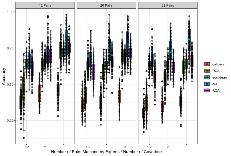
Figure 1: Matching Accuracy in Weighted Euclidean Distance Setting

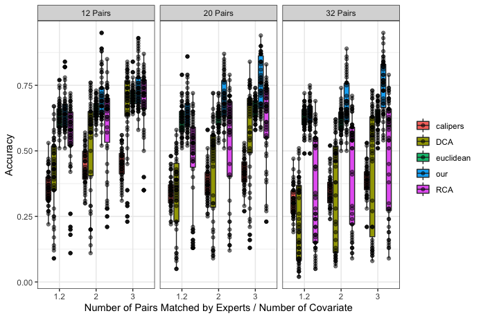
Figure 2: Matching Accuracy in Conjunctive Rules Setting

3.1.2 Algorithm Robustness

We observed from previous subsection that the SCOTOMA possesses 2 great performance properties when all assumptions were satisfied.

• The matching accuracy improves when the signal strength increases while the noise level is kept the same.

• When both the noise level and signal strength are kept the same, the matching accuracy does not deteriorate when the number of dimension increases.

Under the conjunctive rule setup, the distribution of matching accuracy is stretched upward instead of being shifted upward when the signal to noise ratio increases. At the mean time, there is no obvious relationship between matching accuracy and number of covariates.

We observed that the first property is only ”partially” kept, while the second property broke down under the conjunctive rule setup when the model assumptions are grossly violated. In this subsection, we look into scenarios when data deviate from model assumptions in a controlled manner, namely when covariates are correlated and when there are interaction effects. The dimension of the simulated data in this section is fixed at $12$.

Though independence between covariates are not explicitly assumed in our algorithm, high correlation between covariates might mislead SCOTOMA to distribute weights to noisy variables that are correlated with the principle confounders. The Figure 3 shows the matching performance when pairwise correlations are present in the data. We see the performance of SCOTOMA is not affected by correlation between covariates across a wide range of correlation strength.

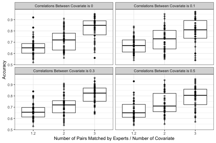
Figure 3:

We also consider the case when the product between principle confounders and other variables are confounders; in this case, the weight of the principle confounders depend on the magnitude of other variables. Order-two interactions between principle confounders and noise variables were randomly picked and included in the underlying weighted Euclidean distance. All interaction terms have weight $0.2$, and the number of interactions is a proportion of $p$ as shown in Figure 4.

We observe that the increase rate in matching accuracy decreases when interactions are present. In the extreme case, $40\%$ of the noisy variables have interaction terms with principle confounders, and there is not much gain in increasing the number of training pairs.

In addition, the max matching accuracy that we observe drops if any interaction is present. This is expected as SCOTOMA cannot assign weights to unobserved variables.

Lastly, the matching accuracy increases when the interaction terms are added and the signal to noise ratio is kept the same. Since the only new information source is the interaction terms, this suggests SCOTOMA learns from the interactions and assigns more weight to relevant variables even when the number of unobserved interactions is large. This hypothesis is also confirmed by the simulation results. We fetch the estimated weights of noisy variables and compare the magnitudes of those which are included in some interaction terms against those which are not. Their averaged differences in each simulation set up are shown by the table below. In this sense, SCOTOMA is robust against interactions.

# of Training Pairs	# of Interactions	Averaged Differences $\times 10$
15	1	1.39
15	2	1.04
15	3	0.435
15	5	0.406
24	1	2.62
24	2	1.3
24	3	0.948
24	5	0.751
36	1	2.66
36	2	1.17
36	3	1.64
36	5	0.856

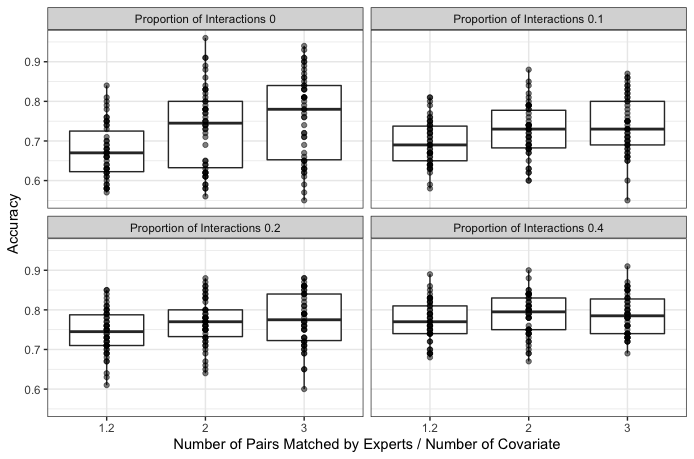
Figure 4:

3.1.3 Self-taught Learning

Lastly, we look at the performance of the self-taught learning framework in the linear setting. We fix the number of matched pairs to be $15$ and change its ratio between the number of unmatched pairs together with the number of covariates. The unmatched observations were simulated from the same distribution of the matched pairs. In each simulation setting, we run the self-taught learning for $10$ iterations $50$ times. The improvement of the matching accuracy is plotted as a function of initial accuracy and shown in blue by the 5. Each point in the plot is the results for one particular simulation; one can tell the procedure rarely suffers from negative learning. In addition, all blue lines have a quadratic shape, which matches our expectation: SCOTOMA gains improvement from self-taught learning only when the initial performance is ”mediocre”.

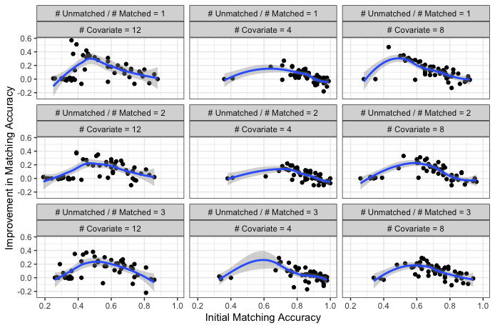
Figure 5:

The question left unanswered is how to find the range of mediocre performance for a specific problem. We recommend users to run the simulation with self-defined simulation parameters that are in line with their own data. One should use the self-taught procedure when the cross-validated performance is higher than the lowest initial accuracy that have an positive, averaged gain should be the and lower than the highest initial accuracy that have an positive, averaged gain. Moreover, one should set an ”accuracy cap” to terminate the self-taught learning procedure when the current performance is higher than the upper bound we just defined.

4 Real Data

We apply the SCOTOMA to a study designed to estimate the longitudinal effect of in-person schooling on SARS-CoV-2 county level transmission as measured by daily case incidence. Based on some inclusion criteria, 229 counties were included in the initial study sample before matching, and 51 pairs of data points were matched by domain experts. We test how well the proposed algorithm can learn replicate experts’ decisions on these 51 pairs. We use all available baseline covariates when performing the SCOTOMA, which include geographical information (ex. state, Bureau of Economic Analysis (BEA) region), school activity level, mask enforcement strength, COVID-19 incidence; in total $13$ variables. Since SCOTOMA take only numerical variables, for geographical indicators, we use the first 2 principal coordinates from multidimensional scaling (Cox and Cox, 2008). The cross-validated matching accuracies of SCOTOMA and its competitors are given in the table below. Euclidean Distance RCA DCA SCOTOMA Matching Accuracy 0.2 0.175 0.175 0.4 Since there are unpaired school districts besides the 51 paired ones, we naturally consider performing the self-taught learning procedure. Running the simulation with suitable parameters, however, suggest running the procedures may not help (see Figure 6). Running the procedure for 10 iterations indeed results in no improvement.

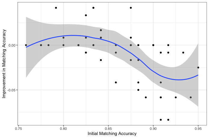
Figure 6:

5 Discussion

SCOTOMA assumes the underlying distance function is a weighted Euclidean distance in the original feature space that is generally not true. Although we have demonstrated SCOTOMA’s robustness against this assumption, it can also be relaxed by simply lifting the design matrix to a richer space. Indicator functions and products of columns could be particularly as they represent decision rules and interactions in the distance function. On the other hand, another notable limitation of SCOTOMA is the number of characterstics must be less than the number of training subjects in each treatment group ($p<\ell$). When the original feature space is ”too rich” ($p<\ell$), one can choose perform suitable dimension-reduction techniques beforehand. The optimal weight from $\eqref{second opt}$ can be interpreted as a ”importance measure” for each variable; this interpretation may not stand when some optimal weights are negative. When this is the case, one may modify (2.3) by adding a linear constrait on $\beta$ so $\hat{\beta}$ is non-negative. In the both of our simulation and real data example, we considered only 1:1 matching. In other settings, when the training pairs are 1:1; generalizations to 1:$k$ matching or full matching are straightforward. When training pairs themselves are 1:$k$, one can use a weighted sum of $k$ sets of objective functions like (2.3) to solve for the optimal $\beta$. However, when performing the semisupervised SCOTOMA; we would reccomend adding 1:1 pairs only to reduce the chance of adding a mis-matched pair.

In this paper, we did not directly analyze the matching accuracy which is the primary performance measure. Asymptotic matching accuracy of $1$ is however, implied by the consistent estimation under mild assumption. We did not theoretically analyze the semisupervised learning framework as we belive the simulation framework provides sufficient and more flexible guidiance to users than simple theoretical results.

To sum up, regular distance-based matching algorithms inevitably fail in high dimensional problems where each study unit has a number of variables. Based on a set of pre-paired training units, our supervised matching algorithm can identify the most important variables and weight them accordingly in the distance measure. Although existed in the literature, this is the first time a ”supervised distance” is used in matching algorithms. Under the model assumptions, this weight estimation is asymptotically consistent. Empirically, it also achives higher matching accurcy than competing methods in both simulated data and real data even when the model assumptions are violated. To make use of the more plentiful unpaired units, we propose a semisupervised companion algorithm which emprically improves the test matching accuracy in most cases. A simulation framwork is also designed to help users determine the potential benefit of this iterative procedure.

Appendix

In appendix, we collect the proofs of lemmas, propositions and theorems appeared in the paper, together with some detailed explanation of contents that might be tedious in the earlier sections.

Input: Training set $X^{T}=(\dot{X}^{T},\ddot{X}^{T})=(\dot{X}_{c}^{T},\dot{X}_{t}^{T},\ddot{X}_{c}^{T},\ddot{X}_{t}^{T})$, Object set $\tilde{X}=(\tilde{X}_{c}^{T},\tilde{X}_{t}^{T})$.

1 Given tuning integers $\tau_{1},\tau_{2}>0$, $k=0$, breakpoint critical value $\Delta_{0}$. The variable importance measure estimate $\hat{\beta}^{(0)}$ is given by (2.3) and define $\dot{\ell}^{(0)}=\dot{\ell}$.

2 Define $\dot{X}_{\iota}^{(0)}=\dot{X}_{\iota}$, $\ddot{X}_{\iota}^{(0)}=\ddot{X}_{\iota}$, $\tilde{X}_{\iota}^{(0)}=\tilde{X}_{\iota}$, $\iota\in\{c,t\}$, and $(\dot{X}^{(0)})^{T}=((\dot{X}_{c}^{(0)})^{T},(\dot{X}_{t}^{(0)})^{T})$.

3 while $\|\hat{\beta}^{(k+1)}-\hat{\beta}^{(k)}\|_{\infty}>\Delta_{0}$, do

4       for $1\leq s\leq\tau_{1}$, do

5            Search the pair of observations, with one from $\ddot{X}_{c}^{(k)}$ and the other from $\ddot{X}_{t}^{(k)}$, such that their score difference with respect to $\hat{\beta}^{(k)}$ is the smallest among all the pairs, i.e.,

$$S_{\hat{\beta}^{(k)}}\big{(}\ddot{x}_{c,i_{s}},\ddot{x}_{t,j_{s}}\big{)}=\min_{\ddot{x}_{c,i}\in\ddot{X}_{c}^{(k)},\ddot{x}_{t,j}\in\ddot{X}_{t}^{(k)}}S_{\hat{\beta}^{(k)}}\big{(}\ddot{x}_{c,i},\ddot{x}_{t,j}\big{)}.$$

6             Update $\ddot{X}_{c}^{(k)}=\ddot{X}_{c}^{(k)}-\{\ddot{x}_{c,i_{s}}\}$ and $\ddot{X}_{t}^{(k)}=\ddot{X}_{t}^{(k)}-\{\ddot{x}_{t,j_{s}}\}$.

7       end for

8      Repeat the above for-loop with $\tau_{1}$ replaced by $\tau_{2}$, $\ddot{X}_{c}^{(k)}$ replaced by $\tilde{X}_{c}^{(k)}$, and $\ddot{X}_{t}^{(k)}$ replaced by $\tilde{X}_{t}^{(k)}$, using indexes $i^{\prime}_{s}$ and $j^{\prime}_{s}$ instead of $i_{s}$ and $j_{s}$ for $1\leq s\leq\tau_{2}$.

9       Update $\big{(}\dot{X}_{c}^{(k+1)}\big{)}^{T}=\big{(}(\dot{X}_{c}^{(k)})^{T},\ddot{x}_{c,i_{1}}^{T},\cdots,\ddot{x}_{c,i_{\tau_{1}}}^{T},\tilde{x}_{c,i^{\prime}_{1}}^{T},\cdots,\tilde{x}_{c,i^{\prime}_{\tau_{2}}}^{T}\big{)}$, and similarly Update $\big{(}\dot{X}_{t}^{(k+1)}\big{)}^{T}=\big{(}(\dot{X}_{t}^{(k)})^{T},\ddot{x}_{t,j_{1}}^{T},\cdots,\tilde{x}_{t,j^{\prime}_{\tau_{2}}}^{T}\big{)}$, Define $\dot{\ell}^{(k+1)}$ = $\dot{\ell}^{(k)}+\tau_{1}+\tau_{2}$.

10       Define $\ddot{X}_{c}^{(k+1)}=\ddot{X}_{c}^{(k)}-\{\ddot{x}_{c,i_{s}}\}_{1\leq s\leq\tau_{1}}$, and $\ddot{X}_{t}^{(k+1)}=\ddot{X}_{t}^{(k)}-\{\ddot{x}_{t,j_{s}}\}_{1\leq s\leq\tau_{1}}$. Similarly Define the $\tilde{X}_{\iota}^{(k+1)}$, $\iota\in\{c,t\}$.

11       Define $(\dot{X}^{(k+1)})^{T}=((\dot{X}_{c}^{(k+1)})^{T},(\dot{X}_{t}^{(k+1)})^{T})$, and Calculate $\hat{\beta}^{(k+1)}$ through (2.3) with $\dot{X}$ replaced by $\dot{X}^{(k+1)}$. Set $k=k+1$.

12 end while

13Let $\hat{\beta}=\hat{\beta}^{(k)}$.

14 Pairing the rest observations within $\tilde{X}$ the same way in algorithm 1 with a critical value $\epsilon>0$.

Output: Variance importance measure estimate $\hat{\beta}$ and the pairing results for the semisupervised training set, given as $\dot{X}^{(k)}$, and for the object set, given as $\mathcal{M}_{out}$.

Algorithm 2 : SCOTOMA in self-taught framework

Proof of Proposition 2.2.

Notice that both $L_{w}$ and $L_{b}$ are positive definite and symmetric, so for the positive definite and symmetric matrix $\Sigma_{w}=\dot{X}^{T}L_{w}\dot{X}/\dot{\ell}+\lambda I$, we may decompose it to $\Sigma_{w}=\Gamma_{\sigma w}\Lambda_{\sigma w}\Gamma_{\sigma w}^{T}$ where $\Gamma_{\sigma w}$ is orthonormal and $\Lambda_{\sigma w}=diag(\lambda_{w1},\cdots,\lambda_{wp})$ is a diagonal matrix with $\lambda_{wi}\geq 0$, $i=1,\cdots,p$. Define $\Lambda_{\sigma w}^{1/2}=diag(\lambda_{w1}^{1/2},\cdots,\lambda_{wp}^{1/2})$, $\Sigma_{w}^{1/2}=\Gamma_{\sigma w}\Lambda_{\sigma w}^{1/2}\Gamma_{\sigma w}^{T}$, and $\eta_{w}=\Sigma_{w}^{1/2}\beta/\|\Sigma_{w}^{1/2}\beta\|_{2}$, we have

$$g(\beta)=\frac{\beta^{T}\dot{X}^{T}L_{b}\dot{X}\beta/\dot{\ell}^{2}}{\beta^{T}\big{(}\dot{X}^{T}L_{w}\dot{X}/\dot{\ell}+\lambda I\big{)}\beta}=\frac{1}{\dot{\ell}^{2}}\eta^{T}_{w}\big{(}\Sigma_{w}^{-1/2}\big{)}^{T}\Sigma_{b}\Sigma_{w}^{-1/2}\eta_{w}.$$

Since the matrix $\big{(}\Sigma_{w}^{-1/2}\big{)}^{T}\Sigma_{b}\Sigma_{w}^{-1/2}$ is again positive definite and symmetric, we may decompose it to $\Gamma\Lambda\Gamma^{T}$ and define $\eta=\Gamma^{T}\eta_{w}$, where $\Gamma$ is an orthonormal matrix and $\Lambda=diag(\lambda_{1},\cdots,\lambda_{p})$ is a diagonal matrix with $\lambda_{1}\geq\lambda_{2}\geq\cdots\geq\lambda_{p}\geq 0$. Hence

$$g(\beta)=\frac{1}{\dot{\ell}^{2}}\eta_{w}^{T}\Sigma\Lambda\Sigma^{T}\eta_{w}=\frac{1}{\dot{\ell}^{2}}\eta^{T}\Lambda\eta\leq\frac{\lambda_{1}}{\dot{\ell}^{2}}\|\eta\|_{2}^{2}=\frac{\lambda_{1}}{\dot{\ell}^{2}}.$$ (A.1)

The equality sign of equation (A.1) holds if and only if $\eta=(1,0,\cdots,0)^{T}$, which means $\eta_{w}$ is the eigenvector of $\big{(}\Sigma_{w}^{-1/2}\big{)}^{T}\Sigma_{b}\Sigma_{w}^{-1/2}$ corresponding to its largest eigenvalue, and leads to the fact that $\beta$ is the eigenvector of $\Sigma_{w}^{-1}\Sigma_{b}$ correspondingly to its largest eigenvalue. ∎

Lemma A.1.

Suppose $P\triangleq(P_{0},P_{1})$ and $Q\triangleq(Q_{0},Q_{1})$ are square orthonormal matrices. where $P_{0},Q_{0}\in\mathcal{M}_{p\times 1}$ and $P_{1},Q_{1}\in\mathcal{M}_{(p-1)\times p}$. Then for $dist(P_{0},Q_{0})$ defined as $dist(P_{0},Q_{0})\triangleq\|P_{0}P_{0}^{T}-Q_{0}Q_{0}^{T}\|_{2}$, we have

$$dist(P_{0},Q_{0})=\|P_{1}^{T}Q_{0}\|_{2}=\|Q_{1}^{T}P_{0}\|_{2}$$

Proof of Lemma A.1.

Define $P_{0}^{T}Q_{0}=\cos\theta$ with some $\theta\in[0,\pi]$ since $P_{0}$ and $Q_{0}$ are unit vectors. Thus

$$\|P_{1}^{T}Q_{0}\|_{2} =\left(\|Q_{0}^{T}P_{1}P_{1}^{T}Q_{0}\|_{2}\right)^{1/2}=\left(\|Q_{0}^{T}\big{(}I-P_{0}P_{0}^{T}\big{)}Q_{0}\|_{2}\right)^{1/2}$$ (A.2)

$$=(1-\cos^{2}\theta)^{1/2}=\sin\theta.$$

The singular value decomposition further implies that, there exist an orthonormal matrix $\tilde{U}$ such that, $Q_{0}^{T}P_{1}=(\sin\theta,0,\cdots,0)\cdot\tilde{U}^{T}$. Therefore,

$$P_{0}P_{0}^{T}-Q_{0}Q_{0}^{T} =P_{0}P_{0}^{T}-(P_{0},P_{1})\begin{pmatrix}P_{0}^{T}\\ P_{1}^{T}\end{pmatrix}Q_{0}Q_{0}^{T}(P_{0},P_{1})\begin{pmatrix}P_{0}^{T}\\ P_{1}^{T}\end{pmatrix}$$

$$=P_{0}P_{0}^{T}-(P_{0},P_{1})\begin{pmatrix}\cos\theta\\ \tilde{U}\begin{pmatrix}\sin\theta\\ 0_{(p-1)\times 1}\end{pmatrix}\end{pmatrix}\begin{pmatrix}\cos\theta,(\sin\theta,0_{1\times(p-1)})\tilde{U}^{T}\end{pmatrix}\begin{pmatrix}P_{0}^{T}\\ P_{1}^{T}\end{pmatrix}$$

$$=(P_{0},P_{1})\begin{pmatrix}1&0\\ 0&\tilde{U}\end{pmatrix}\begin{pmatrix}\begin{pmatrix}\sin^{2}\theta&-\cos\theta\sin\theta\\ -\cos\theta\sin\theta&-\sin^{2}\theta\end{pmatrix}&0_{2\times(p-2)}\\ 0_{(p-2)\times 2}&0\end{pmatrix}\begin{pmatrix}1&0\\ 0&\tilde{U}\end{pmatrix}\begin{pmatrix}P_{0}^{T}\\ P_{1}^{T}\end{pmatrix}.$$

Hence

$$\|P_{0}P_{0}^{T}-Q_{0}Q_{0}^{T}\|_{2}=\|\begin{pmatrix}\sin^{2}\theta&-\cos\theta\sin\theta\\ -\cos\theta\sin\theta&-\sin^{2}\theta\end{pmatrix}\|_{2}=\sin\theta$$ (A.3)

Combine (A.3) with equation (A.2) leads to the result and we proved the lemma. ∎

Proof of Theorem 2.3.

According to Proposition 2.2, $\hat{\beta}^{(0)}$ is the eigenvector of $G_{0}=\Sigma_{w0}^{-1}\Sigma_{b0}$ corresponding to its largest eigenvalue, where

$$\Sigma_{w0} =\lambda I+\frac{1}{\dot{\ell}}\sum_{(\dot{x}_{c,i},\dot{x}_{t,j})\in\mathcal{S}_{0}}(\dot{x}_{c,i}-\dot{x}_{t,j})(\dot{x}_{c,i}-\dot{x}_{t,j})^{T},$$

$$\Sigma_{b0} =\sum_{x\in\dot{X}_{c},y\in\dot{X}_{t},(x,y)\notin\mathcal{S}_{0}}(x-y)(x-y)^{T}.$$

Similarly, $\hat{\beta}^{*}$ is the eigenvector of $G_{0}=\Sigma_{w0}^{-1}\Sigma_{b0}$ corresponding to its largest eigenvalue, where ∎

Let’s assume the experts are trained on a much larger data set $\tilde{X}=\begin{pmatrix}\tilde{X}_{c}^{T}&\tilde{X}_{t}^{T}\end{pmatrix}^{T},\tilde{X}_{c}=\begin{pmatrix}X_{c}^{T}&\bar{X}_{c}^{T}\end{pmatrix}^{T}\ \text{and}\ \tilde{X}_{t}=\begin{pmatrix}X_{t}^{T}&\bar{X}_{t}^{T}\end{pmatrix}^{T}$. Here $X_{c},X_{t}$ are the training data available to us, while $\bar{X}_{c},\bar{X}_{t}$ are training data for experts that is unknown to us.

When all assumptions are met, we would expect the weight vector obtained from the training data is asymptotically the same as the weight vector used by the experts. Define the function

$$G(X)=(X^{T}L_{w}X+\lambda I_{p})^{-1}X^{T}L_{b}X$$

The claim above can be translated to the first eigenvector of $G(X)$ (denoted by $\hat{\beta}$) is the same as the first eigenvector of $G(\tilde{X})$ (denoted by $\beta^{*}$). This is proved based on the Davis-Kahan $\sin(\theta)$ Theorem. Define $dist(X,Z)=||XX^{T}-ZZ^{T}||$, we have

$$dist(\hat{\beta},\beta^{*})\leq\frac{||H||_{2}}{\lambda_{p}(G(X))-||H||_{2}}$$

Here $\lambda_{p}(G(X))$ is the $p^{th}$ eigenvalue of $G(X)$ while $H:=G(X)-G(\tilde{X})$. We firstly prove that $\lambda_{p}$ is bounded from below and then prove $||H||_{2}\overset{p}{\rightarrow}0$. The congvergence rate is $O_{p}(p\log p/\ell_{1})$ or $O_{p}(p/\ell_{1})$ depending on the distribution assumption on feature vectors. The proof of the Davis-Kahan $\sin(\theta)$ Theorem can be found in standard references, we provide a proof for our version in the next section.

We consider the regime where $\ell,\ell_{1},p\rightarrow\infty$ and $0<\ell/\ell_{1}<\infty$, start with an assumption on the feature vectors.

Assumption 1.

For all random observation vectors $X_{c,k},X_{t,k}$ in $X_{c}$, $X_{t}$; we have $E(X_{t,k})=E(X_{c,k})=0$ and $Var(X_{c,k})=Var(X_{t,k})=\Sigma$ such that $||X_{c,k}||\leq\sqrt{p}$ and $||X_{t,k}||\leq\sqrt{p}$ almost surely. Moreover, the smallest eigenvalue of $\Sigma$ is bounded from below.

The key quantitiy $G(X)$ can be decomposed in the following way.

$$G(X) =\frac{1}{\ell}(X^{T}L_{w}X+\lambda I)^{-1}X^{T}(-L_{w}+(k+1)I)X$$ (A.4)

$$=\underbrace{\frac{1}{\ell}(X^{T}L_{w}X+\lambda I)^{-1}X^{T}(-L_{w})X}_{G_{1}(X)}+\underbrace{(X^{T}L_{w}X+\lambda I)^{-1}X^{T}X}_{G_{2}(X)}$$ (A.5)

Define another important quantity

$$\hat{\Sigma}_{\ell_{1}}:=X^{T}(-L_{w}+(k+1)I_{2l})X=\frac{1}{2\ell_{1}}\sum_{k=1}^{2\ell_{1}}\Big{(}X_{c,k}-X_{t,k}\Big{)}^{T}\cdot\Big{(}X_{c,k}-X_{t,k}\Big{)}$$

Two major results are regarding the convergence of the eigenvalues of $\hat{\Sigma}_{\ell_{1}}$ and $X^{T}X/2\ell_{1}$ are needed for the proof.

Lemma A.2.

The smallest of $\hat{\Sigma}_{\ell_{1}}$ is bounded from below. Moreover,

$$||\hat{\Sigma}_{\ell_{1}}-\Sigma||_{2}=O_{p}(\frac{p\log p}{\ell_{1}})$$

$$||\frac{X^{T}X}{2\ell_{1}}-\Sigma||_{2}=O_{p}(\frac{p\log p}{\ell_{1}})$$

If we further assume $X_{c}$, $X_{t}$ are row-wise $\sigma$-sub-Gaussian random matrices,

$$||\hat{\Sigma}_{\ell_{1}}-\Sigma||_{2}=O_{p}(\frac{p}{\ell_{1}})$$

$$||\frac{X^{T}X}{2\ell_{1}}-\Sigma||_{2}=O_{p}(\frac{p}{\ell_{1}})$$

Proof.

Under assumption 1, the second statement follows directly Corollary 6.20 Hign-Dimentional Statistics by M. J. W. The third statement follows directly from Theorem 6.5 in the same book. We now prove the first statement.

$$\hat{\Sigma}_{\ell_{1}}= \frac{1}{2\ell_{1}}\sum_{k=1}^{2\ell_{1}}\Big{(}X_{c,k}-X_{t,k}\Big{)}^{T}\cdot\Big{(}X_{c,k}-X_{t,k}\Big{)}$$

$$= \frac{1}{\sqrt{2\ell_{1}}}\sum_{k=1}^{2\ell_{1}}\Big{[}\Big{(}X_{c,k}-X_{t,k}\Big{)}^{T}\cdot\Big{(}X_{c,k}-X_{t,k}\Big{)}-2\Sigma\Big{]}/\sqrt{2\ell_{1}}+2\Sigma$$

$$:= K+2\Sigma$$

By Weyl’s Inequality, $\lambda_{p}(\hat{\Sigma}_{\ell_{1}})\geq\lambda_{p}(\Sigma)-||K||_{2}=\lambda_{p}(\Sigma)-O_{p}(p\log p/\ell_{1})$ which is bounded away from zero by assumption 1. ∎

We proceed to prove the $\lambda_{p}(G(X))$, which is the $p^{th}$ eigenvalue of $G(X)$, is bounded away from zero. By Weyl’s inequality, $\lambda_{p}(G(X))\geq\lambda_{p}(G_{2}(X))-||G_{1}(X)||_{2}=1/||G_{2}(X)^{-1}||_{2}-||G_{1}(X)||_{2}$.

$$||G_{2}(X)^{-1}||_{2}= ||[\sum_{k=1}^{2\ell_{1}}\Big{(}X_{c,k}-X_{t,k}\Big{)}^{T}\cdot\Big{(}X_{c,k}-X_{t,k}\Big{)}/\ell_{1}+\lambda I/\ell_{1}](X^{T}X/\ell_{1})^{-1}||_{2}$$

$$\leq ||\sum_{k=1}^{2\ell_{1}}\Big{(}X_{c,k}-X_{t,k}\Big{)}^{T}\ \Big{(}X_{c,k}-X_{t,k}\Big{)}/2\ell_{1}+\lambda I/2\ell_{1}||_{2}||(X^{T}X/\ell_{1})^{-1}||_{2}$$

$$= \frac{\lambda_{1}(\hat{\Sigma}_{\ell_{1}})+\lambda/2\ell_{1}}{\lambda_{p}(\frac{X^{T}X}{2\ell_{1}})}$$

$$||G_{1}(X)||_{2}= ||\frac{\lambda}{\ell_{1}}\Big{[}\sum_{k=1}^{2\ell_{1}}\Big{(}X_{c,k}-X_{t,k}\Big{)}^{T}\cdot\Big{(}X_{c,k}-X_{t,k}\Big{)}+\lambda I_{p}\Big{]}^{-1}-\frac{I_{p}}{\ell_{1}}||_{2}$$

$$\leq ||\frac{\lambda}{2\ell_{1}^{2}}\Big{[}\sum_{k=1}^{2\ell_{1}}\Big{(}X_{c,k}-X_{t,k}\Big{)}^{T}\cdot\Big{(}X_{c,k}-X_{t,k}\Big{)}/2\ell_{1}+\lambda I_{p}/2\ell_{1}\Big{]}^{-1}||_{2}+\frac{1}{\ell_{1}}$$

$$= \frac{\lambda}{2\ell_{1}^{2}}\frac{1}{\lambda_{p}(\hat{\Sigma}_{\ell_{1}})+\lambda/2\ell_{1}}+\frac{1}{\ell_{1}}$$

Thus by lemma A.2,

$$\lambda_{p}(G(X))\geq\frac{\lambda_{p}(\Sigma)}{\lambda_{1}(\Sigma)}$$

We proceed to bound $||H||_{2}$

$$||H||_{2}\leq\underbrace{||G_{1}(\tilde{X})-G_{1}(X)||_{2}}_{\leavevmode\hbox to8.9pt{\vbox to8.9pt{\text{[drawing]}}}}+\underbrace{||G_{2}(\tilde{X})-G_{2}(X)||_{2}}_{\leavevmode\hbox to8.9pt{\vbox to8.9pt{\text{[drawing]}}}}$$

For the first part, we have

$$\leq||\frac{\lambda}{2\ell_{1}^{2}}[\hat{\Sigma}_{\ell_{1}}+\lambda I_{p}]^{-1}-\frac{\lambda}{2\ell^{2}}[\hat{\Sigma}_{\ell}+\lambda I_{p}]^{-1}||_{2}+||I_{p}/\ell_{1}-I_{p}/\ell||_{2}$$

$$\leq||\frac{\lambda}{2\ell_{1}^{2}}[\hat{\Sigma}_{\ell_{1}}+\lambda I_{p}]^{-1}||+||\frac{\lambda}{2\ell^{2}}[\hat{\Sigma}_{\ell}+\lambda I_{p}]^{-1}||_{2}+||I_{p}/\ell_{1}-I_{p}/\ell||_{2}$$

$$\overset{(i)}{=}\frac{\lambda}{2\ell_{1}^{2}}\frac{1}{\lambda_{p}(\hat{\Sigma}_{\ell_{1}})+\lambda/2\ell_{1}}+\frac{\lambda}{2\ell^{2}}\frac{1}{\lambda_{p}(\hat{\Sigma}_{\ell})+\lambda/2\ell}+||I_{p}/\ell_{1}-I_{p}/\ell||_{2}$$

$$=O_{p}(\frac{1}{\ell_{1}^{2}})+O_{p}(\frac{1}{\ell^{2}})+O_{p}(1/\ell_{1}-1/\ell)$$

$$=O_{p}(1/\ell_{1})$$

Where $(i)$ follows from lemma A.2. For the second part,

$$\leq||[(\hat{\Sigma}_{\ell_{1}}+\lambda I/2\ell_{1})^{-1}X^{T}X/2\ell_{1}-((\hat{\Sigma}_{\ell}+\lambda I/2\ell)^{-1}X^{T}X/2\ell]||_{2}$$ (A.6)

$$\leq||(\hat{\Sigma}_{\ell_{1}}+\lambda I_{p}/2\ell_{1})^{-1}X^{T}X/2\ell_{1}-(2\Sigma+\lambda I_{p}/2\ell_{1})^{-1}\Sigma||_{2}$$ (A.7)

$$+||(2\Sigma+\lambda I_{p}/2\ell_{1})^{-1}\Sigma-(2\Sigma+\lambda I_{p}/2\ell)^{-1}\Sigma||_{2}$$ (A.8)

$$+||(2\Sigma+\lambda I_{p}/2\ell)^{-1}\Sigma-(\hat{\Sigma}_{\ell}+\lambda I_{p}/2\ell)^{-1}X^{T}X/2\ell||_{2}$$ (A.9)

Consider the second term (A.8) first, we have

$$||(2\Sigma+\lambda I_{p}/\ell_{1})^{-1}\Sigma-(2\Sigma+\lambda I_{p}/\ell_{2})^{-1}\Sigma||_{2}$$

$$= ||\gamma^{T}(2\Sigma+\lambda I_{p}/\ell_{1})^{-1}\Sigma\gamma-\gamma^{T}(2\Sigma+\lambda I_{p}/\ell_{2})^{-1}\Sigma\gamma||_{2}$$

$$= ||\gamma^{T}[diag(\frac{\lambda_{1}}{\lambda_{1}+\lambda/\ell_{1}},\cdots,\frac{\lambda_{p}}{\lambda_{p}+\lambda/\ell_{1}})$$

$$- diag(\frac{\lambda_{1}}{\lambda_{1}+\lambda/\ell},\cdots,\frac{\lambda_{p}}{\lambda_{p}+\lambda/\ell})]\gamma||_{2}$$

$$= ||\gamma^{T}diag(\frac{\lambda/\ell_{1}-\lambda/\ell}{\lambda_{1}+\lambda/\ell_{1}},\cdots,\frac{\lambda/\ell_{1}-\lambda/\ell}{\lambda_{p}+\lambda/\ell_{1}})\gamma||_{2}$$

$$= O(p/\ell_{1}-p/\ell)=O(p/\ell_{1})$$

The first term (A.7) and the third term (A.9) can be treated in the same manner. Without loss of generality, let’s consider the first term

$$||(\hat{\Sigma}_{\ell_{1}}+\lambda I/2\ell_{1})^{-1}X^{T}X/2\ell_{1}-(2\Sigma+\lambda/\ell_{1}I_{p})^{-1}\Sigma||_{2}$$

$$\leq ||(\hat{\Sigma}_{\ell_{1}}+\lambda I/2\ell_{1})^{-1}(X^{T}X/2\ell_{1}-\Sigma)||_{2}$$ (A.10)

$$+ ||[(\hat{\Sigma}_{\ell_{1}}+\lambda I/2\ell_{1})^{-1}-(2\Sigma+\lambda/\ell_{1}I_{p})^{-1}]\Sigma||_{2}$$ (A.11)

The (A.10) term is easy.

$$\eqref{firfir}\leq||(\hat{\Sigma}_{\ell_{1}}+\lambda I/2\ell_{1})^{-1}||_{2}||(X^{T}X/2\ell_{1}-\Sigma)||_{2}=O(\frac{p\log p}{\ell_{1}})$$

It is by the following lemma (Corollary 6.20 H-D Stat by M. J. W.).

$$P(||\hat{\Sigma}-\Sigma||_{2}>\delta)\leq 2p\exp(-\frac{n\delta^{2}}{2b(||\Sigma||_{2}+\delta)})$$

If we can asume each $x_{i}$ is sub-gaussian, $\eqref{firfir}=O(p/\ell_{1})$. Dealing with (A.11) is more complicated, firstly note that

$$\eqref{firsec}\leq||[(\hat{\Sigma}_{\ell_{1}}+\lambda I/2\ell_{1})^{-1}-(2\Sigma+\lambda/\ell_{1}I_{p})^{-1}]||_{2}||\Sigma||_{2}$$

We only need to bound its first part. Define $A=-\hat{\Sigma}_{\ell_{1}}+2\Sigma,B=2\Sigma+\lambda I_{p}/\ell_{1}$, we can write the first part as

$$||(B-A)^{-1}-B^{-1}||_{2}$$

$$= ||(I_{p}-B^{-1}A)^{-1}B^{-1}-B^{-1}||_{2}$$

$$\leq ||B^{-1}||_{2}||(I_{p}-B^{-1}A)^{-1}-I_{p}||_{2}$$

$$\overset{(i)}{=} ||B^{-1}||_{2}||B^{-1}A+(B^{-1}A)^{2}+\cdots||_{2}$$

$$\leq ||B^{-1}||_{2}||B^{-1}A||_{2}[1+\sum_{k=2}^{\infty}||B^{-1}A||_{2}^{k}]$$

$$\overset{(ii)}{\leq} 2||B^{-1}||_{2}||B^{-1}A||_{2}$$

$$\leq ||B^{-1}||_{2}||B^{-1}_{2}||_{2}||A||_{2}$$

$$\overset{(iii)}{=} O_{p}(\frac{p\log p}{\ell_{1}})$$

We have proved $||H||_{2}=O_{p}(p\log p/\ell_{1})$; and $||H||_{2}=O_{p}(p/\ell_{1})$ if the assumption in lemma A.2 is met.

Theorem A.3 (The Davis-Kahan $\sin(\theta)$ Theorem).

Consider $2$ symmetric matrix $G,\hat{G}=G+H\in R^{p\times p}$ with eigen-decompositions

$$G=\sum_{i=1}^{p}\lambda_{i}u_{i}u_{i}^{T}\ \ \ \hat{G}=\sum_{i=1}^{p}\hat{\lambda}_{i}\hat{u}_{i}\hat{u}_{i}^{T}$$

where $\lambda_{1}\geq\cdots\geq\lambda_{p}$; $\hat{\lambda}_{1}\geq\cdots\geq\hat{\lambda}_{p}$ and we write

$$G =\begin{pmatrix}U_{0}&U_{1}\end{pmatrix}\begin{pmatrix}\Lambda_{0}&0\\ 0&\Lambda_{1}\end{pmatrix}\begin{pmatrix}U_{0}^{T}\\ U_{1}^{T}\end{pmatrix}$$

$$\hat{G} =\begin{pmatrix}\hat{U}_{0}&\hat{U}_{1}\end{pmatrix}\begin{pmatrix}\hat{\Lambda}_{0}&0\\ 0&\hat{\Lambda}_{1}\end{pmatrix}\begin{pmatrix}\hat{U}_{0}^{T}\\ \hat{U}_{1}^{T}\end{pmatrix}$$

Here $U_{0}=\begin{pmatrix}u_{1},\cdots,u_{r}\end{pmatrix},\Lambda_{0}=\text{diag}{\begin{pmatrix}\lambda_{1},\cdots,\lambda_{r}\end{pmatrix}}$, $U_{1},\Lambda_{1},\hat{U}_{0},\hat{\Lambda}_{0},\hat{U}_{1},\hat{\Lambda}_{1}$ are defined in the similar way. Then we have

$$||\hat{U}_{1}^{T}HU_{0}||= ||\hat{U}_{1}^{T}(\hat{U}\hat{\Lambda}\hat{U}^{T}-U\Lambda U^{T})U_{0}||$$

$$= ||\hat{\Lambda}_{1}\hat{U}_{1}^{T}U_{0}-\hat{U}_{1}^{T}U_{0}\Lambda_{0}||$$

$$\geq ||\hat{U}_{1}^{T}U_{0}\Lambda_{0}||-||\hat{\Lambda}_{1}\hat{U}_{1}^{T}U_{0}||$$

$$\geq ||\hat{U}_{1}^{T}U_{0}||\lambda_{r}-||\hat{U}_{1}^{T}U_{0}||||\hat{\Lambda}_{1}||$$

By the Weyl’s Theorem, $\hat{\Lambda}\leq||H||$, combined with the statement above,

$$||\hat{U}_{1}^{T}U_{0}||\leq\frac{||\hat{U}_{1}^{T}HU_{0}||}{\lambda_{r}-||H||}\leq\frac{||\hat{U}_{1}||\ ||HU_{0}||}{\lambda_{r}-||H||}\leq\frac{||HU_{0}||}{\lambda_{r}-||H||}\leq\frac{||H||}{\lambda_{r}-||H||}$$

The next lemma connects $||\hat{U}_{1}^{T}U_{0}||$ with $dist(\hat{U}_{0}^{T},Z_{0})$ and finishes the proof.

References

- Austin (2014) {barticle}[author] \bauthor\bsnmAustin, \bfnmPeter C\binitsP. C. (\byear2014). \btitleA comparison of 12 algorithms for matching on the propensity score. \bjournalStatistics in medicine \bvolume33 \bpages1057–1069. \endbibitem
- Bar-Hillel et al. (2005) {barticle}[author] \bauthor\bsnmBar-Hillel, \bfnmAharon\binitsA., \bauthor\bsnmHertz, \bfnmTomer\binitsT., \bauthor\bsnmShental, \bfnmNoam\binitsN., \bauthor\bsnmWeinshall, \bfnmDaphna\binitsD. and \bauthor\bsnmRidgeway, \bfnmGreg\binitsG. (\byear2005). \btitleLearning a Mahalanobis metric from equivalence constraints. \bjournalJournal of machine learning research \bvolume6. \endbibitem
- Bilenko, Basu and Mooney (2004) {binproceedings}[author] \bauthor\bsnmBilenko, \bfnmMikhail\binitsM., \bauthor\bsnmBasu, \bfnmSugato\binitsS. and \bauthor\bsnmMooney, \bfnmRaymond J\binitsR. J. (\byear2004). \btitleIntegrating constraints and metric learning in semi-supervised clustering. In \bbooktitleProceedings of the twenty-first international conference on Machine learning \bpages11. \endbibitem
- Cox and Cox (2008) {bincollection}[author] \bauthor\bsnmCox, \bfnmMichael AA\binitsM. A. and \bauthor\bsnmCox, \bfnmTrevor F\binitsT. F. (\byear2008). \btitleMultidimensional scaling. In \bbooktitleHandbook of data visualization \bpages315–347. \bpublisherSpringer. \endbibitem
- Fisher (1936) {barticle}[author] \bauthor\bsnmFisher, \bfnmRonald A\binitsR. A. (\byear1936). \btitleThe use of multiple measurements in taxonomic problems. \bjournalAnnals of eugenics \bvolume7 \bpages179–188. \endbibitem
- Giraud (2021) {bbook}[author] \bauthor\bsnmGiraud, \bfnmChristophe\binitsC. (\byear2021). \btitleIntroduction to high-dimensional statistics. \bpublisherCRC Press, (pg. 3-5). \endbibitem
- Globerson and Roweis (2005) {barticle}[author] \bauthor\bsnmGloberson, \bfnmAmir\binitsA. and \bauthor\bsnmRoweis, \bfnmSam\binitsS. (\byear2005). \btitleMetric learning by collapsing classes. \bjournalAdvances in neural information processing systems \bvolume18. \endbibitem
- Han et al. (2007) {barticle}[author] \bauthor\bsnmHan, \bfnmJingfeng\binitsJ., \bauthor\bsnmBerkels, \bfnmBenjamin\binitsB., \bauthor\bsnmDroske, \bfnmMarc\binitsM., \bauthor\bsnmHornegger, \bfnmJoachim\binitsJ., \bauthor\bsnmRumpf, \bfnmMartin\binitsM., \bauthor\bsnmSchaller, \bfnmCarlo\binitsC., \bauthor\bsnmScorzin, \bfnmJasmin\binitsJ. and \bauthor\bsnmUrbach, \bfnmHorst\binitsH. (\byear2007). \btitleMumford–Shah model for one-to-one edge matching. \bjournalIEEE Transactions on Image Processing \bvolume16 \bpages2720–2732. \endbibitem
- Hastie, Buja and Tibshirani (1995) {barticle}[author] \bauthor\bsnmHastie, \bfnmTrevor\binitsT., \bauthor\bsnmBuja, \bfnmAndreas\binitsA. and \bauthor\bsnmTibshirani, \bfnmRobert\binitsR. (\byear1995). \btitlePenalized discriminant analysis. \bjournalThe Annals of Statistics \bvolume23 \bpages73–102. \endbibitem
- Hastie, Tibshirani and Buja (1994) {barticle}[author] \bauthor\bsnmHastie, \bfnmTrevor\binitsT., \bauthor\bsnmTibshirani, \bfnmRobert\binitsR. and \bauthor\bsnmBuja, \bfnmAndreas\binitsA. (\byear1994). \btitleFlexible discriminant analysis by optimal scoring. \bjournalJournal of the American statistical association \bvolume89 \bpages1255–1270. \endbibitem
- Hastie and Tibshirani (1995) {barticle}[author] \bauthor\bsnmHastie, \bfnmTrevor\binitsT. and \bauthor\bsnmTibshirani, \bfnmRobert\binitsR. (\byear1995). \btitleDiscriminant adaptive nearest neighbor classification and regression. \bjournalAdvances in neural information processing systems \bvolume8. \endbibitem
- Hastie and Tibshirani (1996) {barticle}[author] \bauthor\bsnmHastie, \bfnmTrevor\binitsT. and \bauthor\bsnmTibshirani, \bfnmRobert\binitsR. (\byear1996). \btitleDiscriminant analysis by Gaussian mixtures. \bjournalJournal of the Royal Statistical Society Series B: Statistical Methodology \bvolume58 \bpages155–176. \endbibitem
- Hoi, Liu and Chang (2010) {barticle}[author] \bauthor\bsnmHoi, \bfnmSteven CH\binitsS. C., \bauthor\bsnmLiu, \bfnmWei\binitsW. and \bauthor\bsnmChang, \bfnmShih-Fu\binitsS.-F. (\byear2010). \btitleSemi-supervised distance metric learning for collaborative image retrieval and clustering. \bjournalACM Transactions on Multimedia Computing, Communications, and Applications (TOMM) \bvolume6 \bpages1–26. \endbibitem
- Hoi et al. (2006) {binproceedings}[author] \bauthor\bsnmHoi, \bfnmSteven CH\binitsS. C., \bauthor\bsnmLiu, \bfnmWei\binitsW., \bauthor\bsnmLyu, \bfnmMichael R\binitsM. R. and \bauthor\bsnmMa, \bfnmWei-Ying\binitsW.-Y. (\byear2006). \btitleLearning distance metrics with contextual constraints for image retrieval. In \bbooktitle2006 IEEE Computer Society Conference on Computer Vision and Pattern Recognition (CVPR’06) \bvolume2 \bpages2072–2078. \bpublisherIEEE. \endbibitem
- Peng, Ngo and Xiao (2007) {barticle}[author] \bauthor\bsnmPeng, \bfnmYuxin\binitsY., \bauthor\bsnmNgo, \bfnmChong-Wah\binitsC.-W. and \bauthor\bsnmXiao, \bfnmJianguo\binitsJ. (\byear2007). \btitleOM-based video shot retrieval by one-to-one matching. \bjournalMultimedia Tools and Applications \bvolume34 \bpages249–266. \endbibitem
- Raina et al. (2007) {binproceedings}[author] \bauthor\bsnmRaina, \bfnmRajat\binitsR., \bauthor\bsnmBattle, \bfnmAlexis\binitsA., \bauthor\bsnmLee, \bfnmHonglak\binitsH., \bauthor\bsnmPacker, \bfnmBenjamin\binitsB. and \bauthor\bsnmNg, \bfnmAndrew Y\binitsA. Y. (\byear2007). \btitleSelf-taught learning: transfer learning from unlabeled data. In \bbooktitleProceedings of the 24th international conference on Machine learning \bpages759–766. \endbibitem
- Rockafellar (2015) {bbook}[author] \bauthor\bsnmRockafellar, \bfnmRalph Tyrell\binitsR. T. (\byear2015). \btitleConvex analysis. \bpublisherPrinceton university press. \endbibitem
- Rosenbaum and Rubin (1983) {barticle}[author] \bauthor\bsnmRosenbaum, \bfnmPaul R\binitsP. R. and \bauthor\bsnmRubin, \bfnmDonald B\binitsD. B. (\byear1983). \btitleThe central role of the propensity score in observational studies for causal effects. \bjournalBiometrika \bvolume70 \bpages41–55. \endbibitem
- Rosenbaum and Rubin (1985) {barticle}[author] \bauthor\bsnmRosenbaum, \bfnmPaul R\binitsP. R. and \bauthor\bsnmRubin, \bfnmDonald B\binitsD. B. (\byear1985). \btitleConstructing a control group using multivariate matched sampling methods that incorporate the propensity score. \bjournalThe American Statistician \bvolume39 \bpages33–38. \endbibitem
- Schmee (1986) {bmisc}[author] \bauthor\bsnmSchmee, \bfnmJosef\binitsJ. (\byear1986). \btitleAn introduction to multivariate statistical analysis. \endbibitem
- Si et al. (2006) {barticle}[author] \bauthor\bsnmSi, \bfnmLuo\binitsL., \bauthor\bsnmJin, \bfnmRong\binitsR., \bauthor\bsnmHoi, \bfnmSteven CH\binitsS. C. and \bauthor\bsnmLyu, \bfnmMichael R\binitsM. R. (\byear2006). \btitleCollaborative image retrieval via regularized metric learning. \bjournalMultimedia Systems \bvolume12 \bpages34–44. \endbibitem
- Stuart (2010) {barticle}[author] \bauthor\bsnmStuart, \bfnmElizabeth A\binitsE. A. (\byear2010). \btitleMatching methods for causal inference: A review and a look forward. \bjournalStatistical science: a review journal of the Institute of Mathematical Statistics \bvolume25 \bpages1. \endbibitem
- Weinberger and Saul (2009) {barticle}[author] \bauthor\bsnmWeinberger, \bfnmKilian Q\binitsK. Q. and \bauthor\bsnmSaul, \bfnmLawrence K\binitsL. K. (\byear2009). \btitleDistance metric learning for large margin nearest neighbor classification. \bjournalJournal of machine learning research \bvolume10. \endbibitem
- Xing et al. (2002) {barticle}[author] \bauthor\bsnmXing, \bfnmEric\binitsE., \bauthor\bsnmJordan, \bfnmMichael\binitsM., \bauthor\bsnmRussell, \bfnmStuart J\binitsS. J. and \bauthor\bsnmNg, \bfnmAndrew\binitsA. (\byear2002). \btitleDistance metric learning with application to clustering with side-information. \bjournalAdvances in neural information processing systems \bvolume15. \endbibitem