An Alternative Graphical Lasso Algorithm for Precision Matrices

Abstract

The Graphical Lasso (GLasso) algorithm is fast and widely used for estimating sparse precision matrices (Friedman et al., 2008). Its central role in the literature of high-dimensional covariance estimation rivals that of Lasso regression for sparse estimation of the mean vector. Some mysteries regarding its optimization target, convergence, positive-definiteness and performance have been unearthed, resolved and presented in Mazumder and Hastie (2011), leading to a new/improved (dual-primal) DP-GLasso. Using a new and slightly different reparametriztion of the last column of a precision matrix we show that the regularized normal log-likelihood naturally decouples into a sum of two easy to minimize convex functions one of which is a Lasso regression problem. This decomposition is the key in developing a transparent, simple iterative block coordinate descent algorithm for computing the GLasso updates with performance comparable to DP-GLasso. In particular, our algorithm has the precision matrix as its optimization target right at the outset, and retains all the favorable properties of the DP-GLasso algorithm.

Keywords: Convergence, Graphical Models, Optimization Target, Positive-definiteness, Primal-Dual, Sparsity, Tuning Parameters.

1 Introduction

Given the data matrix $\mathbf{Y}_{n\times p}$, a sample of $n$ realizations from a $p$-dimensional Gaussian distribution with zero mean, unknown positive-definite covariance matrix $\Sigma$ and precision matrix $\mbox{\boldmath$\Theta$}=\mbox{\boldmath$\Sigma$}^{-1}$. It is desired to have a sparse estimate of the unknown precision matrix. The popular Graphical Lasso (GLasso) algorithm (Friedman et al., 2008; Banerjee et al., 2008) has played a central role in the literature of high-dimensional covariance and precision matrix estimation and is the benchmark against which the performances of the newer methods are compared with. Its goal is to solve the following $\ell_{1}$-penalized optimiziation problem:

$$\min_{\mbox{\boldmath$\Theta$}}-\log\det(\mbox{\boldmath$\Theta$})+\mbox{tr}(\mathbf{S}\mbox{\boldmath$\Theta$})+\lambda\|\mbox{\boldmath$\Theta$}\|_{1},$$ (1)

over the set of positive-definite matrices $\Theta$, where $\lambda$ is a tuning parameter, $\mathbf{S}$ is the sample covariance matrix of the data and $||\mbox{\boldmath$\Theta$}||_{1}$ is its $\ell_{1}$-norm.

The starting point of Friedman et al. (2008) and Mazumder and Hastie (2011) is the subgradient of (1) given by

$$\mbox{\boldmath$\Theta$}^{-1}-\mathbf{S}-\lambda\boldsymbol{\Gamma}=0,$$ (2)

where $\boldsymbol{\Gamma}$ is the matrix of component-wise sign of the precision matrix $\Theta$. The GLasso algorithm uses a block-coordinate descent method for solving (2) by partitioning the matrices $\Theta$, $\mathbf{S}$, $\mathbf{W}=\mbox{\boldmath$\Theta$}^{-1}$ and $\Gamma$ as

$$\mbox{\boldmath$\Theta$}=\begin{pmatrix}\mbox{\boldmath$\Theta$}_{11}&\boldsymbol{\theta}_{12}\\ \boldsymbol{\theta}_{12}^{{}^{\prime}}&\theta_{22}\end{pmatrix};\;\mathbf{S}=\begin{pmatrix}\mathbf{S}_{11}&\boldsymbol{s}_{12}\\ \boldsymbol{s}_{12}^{{}^{\prime}}&s_{22}\end{pmatrix},$$ (3)

where $\mbox{\boldmath$\Theta$}_{11},\boldsymbol{\theta}_{12}$ are $(p-1)\times(p-1),(p-1)\times 1$, and $\theta_{22}$ is a scalar. More specifically, the GLasso solves for $\mathbf{W}$ in (2) one row/column at a time, while keeping all other entries fixed. It is convenient to focus on the $p$th column which amounts to solving

$$\boldsymbol{w}_{12}-\boldsymbol{s}_{12}-\lambda\boldsymbol{\gamma}_{12}=0,\;w_{22}=(\theta_{22}-\boldsymbol{\theta}_{12}^{\prime}\mbox{\boldmath$\Theta$}_{11}^{-1}\boldsymbol{\theta}_{12})^{-1},$$ (4)

where the first equation is from the last column of (2) and the second equality follows from the identity $\mathbf{W}\mbox{\boldmath$\Theta$}=\boldsymbol{I}$. One of the several issues pointed out in Mazumder and Hastie (2011, Section 2) is that repeated use of (4) in the GLasso updating iterations violates the requirement of ”keeping all other entries fixed”. More generally, presence of $\mathbf{W}=\mbox{\boldmath$\Theta$}^{-1}$ in (2) seems unnatural and possibly the main source of confusion and mysteries associated with GLasso as highlighted, resolved and explained cogently in Mazumder and Hastie (2011). Curiously, relying on (2) seems to keep around the ghost of $\mathbf{W}$ and the need for going back and forth between primal and dual formulations. Thus, it is natural to ask: Is it possible to bypass (2) or $\mathbf{W}$ in deriving the GLasso updates?

In this paper, we provide an affirmative answer by showing that simply working with the partitioned $\Theta$ in (1) suggests a new reparametrization of its last column and paves the way to decouple the objective function as a sum of two convex functions. The ensuing decoupled subgradients are much simpler than (2), and the key to avoiding it along with $\mathbf{W}$. Thus, dispelling almost effortlessly the mysteries around deriving the GLasso updates. The new reparametrization of the last column of $\Theta$ as $(\boldsymbol{\theta}_{12},\gamma),\gamma=\theta_{22}-\boldsymbol{\theta}_{12}^{{}^{\prime}}\mbox{\boldmath$\Theta$}_{11}^{-1}\boldsymbol{\theta}_{12}$, is different from $(\boldsymbol{\theta}_{12}/\theta_{22},w_{22})$ employed in Mazumder and Hastie (2011). In fact, here $\gamma=w_{22}^{-1}$ has the interpretation as the residual variance of regressing $Y_{p}$ on the other variables, but $-\boldsymbol{\theta}_{12}/\theta_{22}$ is the corresponding regression coefficients.

Our derivation of the updates and the ensuing S-GLasso algorithm presented in Section 2, is inspired by an algorithm in Wang (2014) for regularized estimation of covariance matrices which leads to bi-convex objective functions. It turns out that the key reparametrization idea in Wang (2014) works even better for regularized estimation of precision matrices where the objective function turns out to be convex in the new parameters $(\boldsymbol{\theta}_{12},\gamma)$.

For completeness, we provide the derivation and necessary steps of the classic GLasso algorithm in Section A of the Supplementary Material.

2 A Direct Derivation of GLasso Updates

Whereas GLasso starts with the subgradients (2) and then focuses on updating the last row/column of $\mathbf{W}$ using (4), we first decouple the objective function (1) to obtain simpler subgradients involving directly the components of $\Theta$. Then, focus on updating its last row/column using the reparametrizations

$$\boldsymbol{\beta}=\boldsymbol{\theta}_{12},\ \gamma=\theta_{22}-\boldsymbol{\beta}^{{}^{\prime}}\mbox{\boldmath$\Theta$}_{11}^{-1}\boldsymbol{\beta},$$ (5)

where the new parameters are different from their counterparts in (4).

2.1 Decoupling the Penalized Likelihhod

We show that using the new parameters in (5) the penalized (negative) normal log-likelihood function magically decouples as a sum of two convex functions of $\gamma$ and $\boldsymbol{\beta}$. Indeed, it follows after some straightforward algebra that:

$$1) \log\det(\mbox{\boldmath$\Theta$})=\log(\gamma)+c,$$ (6)

$$2) \mbox{tr}(\mathbf{S}\mbox{\boldmath$\Theta$})=2\boldsymbol{s}_{12}^{{}^{\prime}}\boldsymbol{\beta}+s_{22}(\gamma+\boldsymbol{\beta}^{{}^{\prime}}\mbox{\boldmath$\Theta$}_{11}^{-1}\boldsymbol{\beta})+c,$$

$$3) \|\mbox{\boldmath$\Theta$}\|_{1}=2\|\boldsymbol{\beta}\|_{1}+\gamma+\boldsymbol{\beta}^{{}^{\prime}}\mbox{\boldmath$\Theta$}_{11}^{-1}\boldsymbol{\beta}+c,$$

where $c$ is a universal constant; for a proof, see Section B of the Supplementary Material. Thus, ignoring the constants, plugging these in (1) and rearranging terms, it turns out that the objective function in (1) decouples in $\gamma$ and $\boldsymbol{\beta}$ as

$$\min_{\gamma,\boldsymbol{\beta}}\;\{-\log\gamma+(s_{22}+\lambda)\gamma\}+\{(s_{22}+\lambda)\boldsymbol{\beta}^{{}^{\prime}}\mbox{\boldmath$\Theta$}_{11}^{-1}\boldsymbol{\beta}+2\boldsymbol{s}_{12}^{{}^{\prime}}\boldsymbol{\beta}+2\lambda\|\boldsymbol{\beta}\|_{1}\}.$$ (7)

The function is convex in $\boldsymbol{\alpha}=[\gamma,\boldsymbol{\beta}^{{}^{\prime}}]^{{}^{\prime}}$ being a sum of two convex functions, and minimization over $\boldsymbol{\beta}$ of the second sum is easily recognized as a Lasso regression or quadratic programming problem.

2.2 A Simple GLasso (S-GLasso) Algorithm

The updates for our new S-GLasso algorithm are derived through minimization of the two components of the decoupled objective function.

First, solving (7) by minimizing it with respect to $\gamma$ gives

$$\gamma=\frac{1}{s_{22}+\lambda}.$$ (8)

Similarly, for $\boldsymbol{\beta}$ with ${\boldsymbol{V}}=(s_{22}+\lambda)\Theta_{11}^{-1}$, we need to solve

$$\min_{\boldsymbol{\beta}}\;\boldsymbol{\beta}^{{}^{\prime}}{\boldsymbol{V}}\boldsymbol{\beta}+2\boldsymbol{s}_{12}^{{}^{\prime}}\boldsymbol{\beta}+2\lambda\|\boldsymbol{\beta}\|_{1},$$ (9)

which is recognized as a Lasso regression problem. The solution for its $j$-th element $\beta_{j}$ is known (Friedman et al., 2008, Equation 11) to be given by

$$\beta_{j}=\frac{S(-[(\boldsymbol{s}_{12})_{j}+\sum_{k\neq j}v_{jk}\beta_{k}],\lambda)}{v_{jj}},$$ (10)

where $S(\cdot,\lambda)$ is a soft-thresholding operator and the tuning parameter $\lambda$ controls the sparseness of the solution. The update (10) is iterated for $j=1,2\ldots,p-1,1,2\ldots$ till convergence. These are the two key steps for computing the updates in our Algorithm 1 or the S-GLasso given next.

Algorithm 1 S-GLasso

1.  Initialize $\mbox{\boldmath$\Theta$}^{(0)}=(\mbox{diag}(\mathbf{S})+\lambda\boldsymbol{I})^{-1}$, for a given $\lambda$,

2.   Repeat for $i=1$ to $p$ until convergence,

a.   Partition $\mbox{\boldmath$\Theta$}^{(k)}$ and $\mathbf{S}$ as in (3),

b.   Compute $\gamma$ as in (8),

c.   Solve the Lasso regression (9) by repeating (10) until convergence,

d.   Update $\boldsymbol{\theta}_{12}^{(k+1)}=\boldsymbol{\beta},\,\theta_{22}^{(k+1)}=\gamma+\boldsymbol{\beta}^{{}^{\prime}}\mbox{\boldmath$\Theta$}_{11}^{-1}\boldsymbol{\beta}$,

3.  Output $\Theta$.

The preceding development shows that it is, indeed, possible to bypass (2) or $\mathbf{W}$ in deriving the GLasso updates. The rest of the paper more or less follows Mazumder and Hastie (2011) to speed up the computation, and to compare S-GLasso with DP-Lasso and GLasso.

2.3 Speeding up the S-GLasso

The iterations in (10) requires inverting the matrix $\mbox{\boldmath$\Theta$}_{11}$ which is computationally expensive when $p$ is large. Thus, to speed up the S-GLasso algorithm we follow closely the steps in Mazumder and Hastie (2011) and solve the dual of (9), as a box-constrained quadratic programming with constraints $u_{i}\in[-\lambda,\lambda]$ for $i=1,\dots,p-1$:

$$\min_{\boldsymbol{u}} \;\frac{1}{2}(\boldsymbol{s}_{12}+\boldsymbol{u})^{{}^{\prime}}\mbox{\boldmath$\Theta$}_{11}(\boldsymbol{s}_{12}+\boldsymbol{u}),$$ (11)

s.t. $$u_{i}\in[-\lambda,\lambda];\;i=1,\dots,p-1.$$

The latter can be solved using the coordinate descent algorithm giving the optimal $\hat{\boldsymbol{u}}$. Then, we incorporate these modifications by substituting the substeps (c) and (d) in the Algorithm 1 by

1. Solve the dual (11) by coordinate descent and compute $\boldsymbol{\beta}=\mbox{\boldmath$\Theta$}^{(k+1)}_{11}(\boldsymbol{s}_{12}+\hat{\boldsymbol{u}})/(s_{22}+\lambda)$,

2. Update $\boldsymbol{\theta}_{12}^{(k+1)}=\boldsymbol{\beta},\,\theta^{(k+1)}_{22}=\gamma+(\boldsymbol{s}_{12}+\hat{\boldsymbol{u}})^{{}^{\prime}}\boldsymbol{\beta}/{(s_{22}+\lambda)}$.

It is shown in Section C of the Supplementary Material that $\boldsymbol{\beta}$ and $\gamma$ can be computed from the optimal $\hat{\boldsymbol{u}}$ via $\boldsymbol{\beta}=\mbox{\boldmath$\Theta$}_{11}(\boldsymbol{s}_{12}+\hat{\boldsymbol{u}})/(s_{22}+\lambda)$. Then we update the row/column of $\Theta$ as $\boldsymbol{\theta}_{12}=\boldsymbol{\beta}$ and $\theta_{22}=\gamma-(\boldsymbol{s}_{12}+\hat{\boldsymbol{u}})^{{}^{\prime}}\boldsymbol{\beta}/{(s_{22}+\lambda)}.$

2.4 Connections with DP-GLasso

A comprehensive list of advantages of DP-GLasso over the traditional GLasso is provided in Mazumder and Hastie (2011). Here, our focus is on highlighting some of the similarities and differences of GLasso, DP-GLasso and S-GLasso as summarized in Table 1 (Also see Figure 5 of the Supplementary Material).

The key difference between S-GLasso and DP-GLasso is in the derivation of the updates. While DP-GLasso employs (2) and the matrix $\boldsymbol{W}$, S-GLasso utilizes the new parameters and the decoupled (1) to compute $\Theta$ directly, thus obviates the need for $\boldsymbol{W}$. Despite this difference, S-GLasso and DP-GLasso algorithms both employ block coordinate descent optimization to minimize the primal objective function, while GLasso minimizes the dual of (1). Another beneficial property shared with DP-GLasso is the maintenance of positive definiteness of $\mbox{\boldmath$\Theta$}^{(k+1)}$ in each iteration, as long as the initial matrix $\mbox{\boldmath$\Theta$}^{(0)}$ is positive-definite, as the matrix ${\mbox{\boldmath$\Theta$}^{(k)}_{11}}$ remains fixed during a row/column update, and $\gamma$ is positive. For further details, refer to Mazumder and Hastie (2011, Lemma 4).

Table 1: Comparison of GLasso, DP-GLasso and S-GLasso

	GLasso	DP-GLasso	S-GLasso
$\Theta$ optim. target	✗	✓	✓
$\Theta$ always P.D.	✗	✓	✓
Always Converge	✗	✓	✓
Monotone	✗	✓	✓

So far as convergence is concerned, Algorithm 1 is an unconstrained block coordinate descent algorithm with $p$-blocks of $\boldsymbol{\alpha}=[\gamma,\boldsymbol{\beta}^{{}^{\prime}}]^{{}^{\prime}}$. Its convergence to the stationary point follows from the Tseng (2001, Thereom 4.1 and Lemma 4.1), since the non-differentiable penalty term is separable, the objective function has a unique minimum point in each coordinate block and the directional derivatives exist. Moreover, since (1) is convex the convergence to a global minimum is guaranteed.

3 Simulation Results

In this section, we compare the performance of S-GLasso with the DP-GLasso algorithm. For the latter, we use the R package dpglasso.

Experiment 1: We employ the function huge.generator() from the huge package to generate population precision matrices with approximately 70% of the entries being zero, considering various combinations of $(n,p)$.

• $p=200,\,n\in\{50,200,500\}$

• $p=500,\,n\in\{200,500,800\}$

• $p=800,\,n\in\{500,800,1000\}$

• $p=1000,\,n\in\{500,1000,1500\}$

Similar to (Mazumder and Hastie, 2011), we implement S-GLasso and DP-GLasso for every combination of $(n,p)$ on a grid of twenty linearly spaced $\lambda$ values, where $\lambda_{i}=0.8^{i}(0.9\lambda_{\max})\,,i=1,\dots,20$, using a cold start initialization, i.e. $\mbox{\boldmath$\Theta$}^{(0)}=(\mbox{diag}(\mathbf{S})+\lambda\boldsymbol{I})^{-1}$ (for additional results using warm start initalization, see Supplementary Material). Here, $\lambda_{\max}$ is the maximum of the non-diagonal elements of $\mathbf{S}$ and corresponds to the smallest value for which $\Theta$ is a diagonal matrix.

To compare the performance of the two algorithms, we use two measures: area under the curve (AUC) and the number of iterations until convergence. Similar to the convergence criterion in the dpglasso package, we consider the algorithm to have converged if the relative difference in the Frobenius norm of the precision matrices across two successive iterations is less than $1e-4$. Figure 1 and Table 2 summarize the results. In Figure 1, rows and columns correspond to different combinations of $p$ and $n$, respectively.

Table 2: AUC score for S-GLasso and DP-GLasso

p	n	S-GLasso	DP-GLasso
200	50	0.46738	0.41331
	200	0.59471	0.59471
	500	0.70403	0.70403
500	200	0.49915	0.49850
	500	0.59581	0.59579
	800	0.64664	0.64663
800	500	0.54609	0.54608
	800	0.59489	0.59488
	1000	0.61594	0.61594
1000	500	0.54609	0.54608
	1000	0.59489	0.59488
	1500	0.61594	0.61594

As shown in Table 2, S-GLasso and DP-GLasso report similar results. The findings in Figure 1 corroborate earlier results, indicating that S-GLasso and DP-GLasso are highly comparable. Specifically, for $\lambda$ values close to 0, DP-GLasso converges slightly faster, but as $\lambda$ values increase, S-GLasso achieves faster convergence.

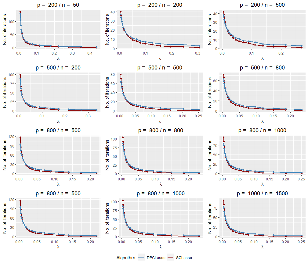
Figure 1: Number of iterations for S-GLasso and DP-GLasso.

Experiment 2 The goal of this experiment is to compare the number of iterations necessary to achieve the convergence of both S-GLasso and DP-GLasso when $\lambda$ is chosen such that the estimated number of zeros of the precision matrix equal to the oracle (i.e. the true precision matrix) and show that S-GLasso and DP-GLasso implement the same graph selection. We use the same data generating process as in the previous experiment and report results only for $p=500,\,n\in\{200,500,800\}$ using cold and warm start initialization. The results of other combinations are similar and not reported here.

To numerically demonstrate that S-GLasso and DP-GLasso yield the same precision matrix, we calculate the Structural Hamming Distance between two estimated precision matrices and their Frobenius norm difference. To mitigate the numerical differences due to machine precision , we threshold both precision matrices at the value equal to $1e-6$, meaning elements with values less than $1e-6$ are set to 0. In all simulation results, both metrics return value 0, indicating that the results of S-GLasso and DP-GLasso are the same. However, our simulations show that both algorithms require a slightly different $\lambda$ values (an average difference of approximately $\pm 0.005$) to achieve the number of zeros equal to the oracle.

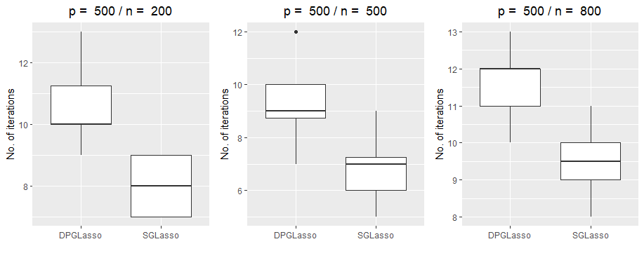
Figure 2: Number of iterations for S-GLasso and DP-GLasso (cold-start).

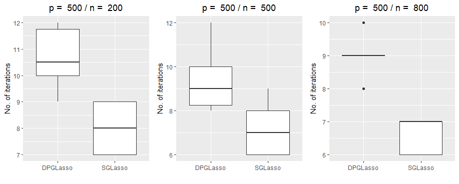
Figure 3: Number of iterations for S-GLasso and DP-GLasso (warm-start).

Figures 2 and 3 report the results for cold and warm start initialization, respectively. As can be seen, for all cases S-GLasso requires a fewer number of observations than DP-GLasso.

Appendix A Details on Graphical Lasso

GLasso uses a block coordinate descent method for solving the ”normal equations” (Friedman et al., 2008)

$$\mbox{\boldmath$\Theta$}^{-1}-\mathbf{S}-\lambda\boldsymbol{\Gamma}=0,$$ (12)

Similar to (3) in the main text, lets consider the partitioning of $\boldsymbol{W}=\mbox{\boldmath$\Theta$}^{-1}$ using a well-known properties of inverse of a block-partitioned matrix

$$\mathbf{W}=\begin{pmatrix}\mathbf{W}_{11}&\boldsymbol{w}_{12}\\ \boldsymbol{w}_{12}^{{}^{\prime}}&w_{22}\end{pmatrix}=\begin{pmatrix}\Big{(}\mbox{\boldmath$\Theta$}_{11}-\frac{\boldsymbol{\theta}_{12}\boldsymbol{\theta}_{12}^{{}^{\prime}}}{\theta_{22}}\Big{)}^{-1}&-\mathbf{W}_{11}\frac{\boldsymbol{\theta}_{12}}{\theta_{22}}\\ -\frac{\boldsymbol{\theta}_{12}^{{}^{\prime}}}{\theta_{22}}\mathbf{W}_{11}&\frac{1}{\theta_{22}}-\frac{\boldsymbol{\theta}_{12}^{{}^{\prime}}\mathbf{W}_{11}\boldsymbol{\theta}_{12}}{\theta_{22}^{2}}.\end{pmatrix}$$ (13)

From the last column of (12), we have $\boldsymbol{w}_{12}-\boldsymbol{s}_{12}-\lambda\boldsymbol{\gamma}_{12}=\boldsymbol{0}$. Plugging $\boldsymbol{w}_{12}=-\mathbf{W}_{11}\boldsymbol{\theta}_{12}/\theta_{22}$ from (13) to the latter equation, we have

$$\mathbf{W}_{11}\boldsymbol{\beta}+\boldsymbol{s}_{12}+\lambda\boldsymbol{\gamma}_{12}=\boldsymbol{0},$$ (14)

where $\boldsymbol{\beta}=\frac{\boldsymbol{\theta}_{12}}{\theta_{22}}$. It turns out (14) is a stationarity equation for the following lasso problem

$$\min_{\boldsymbol{\beta}}\frac{1}{2}\boldsymbol{\beta}^{{}^{\prime}}\mathbf{W}_{11}\boldsymbol{\beta}+\boldsymbol{\beta}^{{}^{\prime}}\boldsymbol{s}_{12}+\lambda\|\boldsymbol{\beta}\|_{1}.$$ (15)

It is important to note that in (15), $\mathbf{W}\succ 0$ is considered as fixed. However, this assumption is violated, since from (13), $\mathbf{W}_{11}$ depends on $\boldsymbol{\theta}_{12}$. This results to the non-monotonic behavior of GLasso.

Given the $\hat{\boldsymbol{\beta}}$, one can easily obtain $\hat{\boldsymbol{w}}_{12}$ from (13) and $\hat{\theta}_{22}=1/(w_{22}-\hat{\boldsymbol{\beta}}^{{}^{\prime}}\hat{\boldsymbol{w}}_{12})$. Finally, $\hat{\boldsymbol{\theta}}_{12}$ can be found from the definition of $\boldsymbol{\beta}$. Now, GLasso moves and updates the next blocks until convergence. Algorithm 2 summarizes the steps.

Algorithm 2 GLasso

1.  Initialize $\mathbf{W}^{(0)}=(\mathbf{S}+\lambda\boldsymbol{I})$

2.   Repeat for $i=1$ to $p$ until convergence

a.   Partition $\mbox{\boldmath$\Theta$}^{(k+1)},\mathbf{W}^{(k+1)}$ and $\mathbf{S}$ as in (13)

b.   Solve the Lasso problem (14)

c.   Compute $\hat{\boldsymbol{w}}_{12}=-\mathbf{W}_{11}\hat{\boldsymbol{\beta}}$

d.   Update $\theta_{22}^{(k+1)}=1/(w_{22}-\hat{\boldsymbol{\beta}}^{{}^{\prime}}\hat{\boldsymbol{w}}_{12})$ and $\boldsymbol{\theta}_{12}^{(k+1)}=\hat{\boldsymbol{\beta}}\theta_{22}^{(k+1)}$

3.  Output $\Theta$

Appendix B Proof of (6)

Proof of Statement 1: From Schur’s determinant identity (Horn and Johnson, 2012), for a square matrix $\Theta$, if $\mbox{\boldmath$\Theta$}_{11}$ is non-singular then

$$\det(\mbox{\boldmath$\Theta$})=\det(\mbox{\boldmath$\Theta$}_{11})\det(\theta_{22}-\boldsymbol{\theta}_{12}^{{}^{\prime}}\mbox{\boldmath$\Theta$}_{11}^{-1}\boldsymbol{\theta}_{12})$$

Recalling, that $\gamma=\theta_{22}-\boldsymbol{\theta}_{12}^{{}^{\prime}}\mbox{\boldmath$\Theta$}_{11}^{-1}\boldsymbol{\theta}_{12}$, the result follows.

Proof of Statement 2: It is straight forward to show that

$$\mbox{diag}(\mathbf{S}\mbox{\boldmath$\Theta$})=(\mathbf{S}_{11}\mbox{\boldmath$\Theta$}_{11}+\boldsymbol{s}_{12}\boldsymbol{\theta}_{12}^{{}^{\prime}},\boldsymbol{s}_{12}^{{}^{\prime}}\boldsymbol{\theta}_{12}+s_{22}\theta_{22})$$

Then, after plugging $\theta_{22}=\gamma+\boldsymbol{\theta}_{12}^{{}^{\prime}}\mbox{\boldmath$\Theta$}_{11}^{-1}\boldsymbol{\theta}_{12}$ and $\boldsymbol{\beta}=\boldsymbol{\theta}_{12}$, the result follows.

Proof of Statement 3: Directly follows from the definition of $\|\cdot\|_{1}$ and the partition in (3).

Appendix C Details on the Dual of (9)

In this section, we derive the dual of the following optimization problem

$$\min_{\boldsymbol{\beta}}\;\frac{1}{2}\boldsymbol{\beta}^{{}^{\prime}}\boldsymbol{V}\boldsymbol{\beta}+s_{12}^{{}^{\prime}}\boldsymbol{\beta}+\lambda\|\boldsymbol{\beta}\|_{1}$$ (16)

Recall that the $\ell_{1}$ norm can be expressed as

$$\lambda\|\boldsymbol{\beta}\|_{1}=\max_{\|\boldsymbol{u}\|_{\infty}\leq\lambda}\boldsymbol{\beta}^{{}^{\prime}}\boldsymbol{u}$$

Substituting this result into (16) and swapping the $\min$ and $\max$

$$\min_{\boldsymbol{\beta}}\; \frac{1}{2}\boldsymbol{\beta}^{{}^{\prime}}\boldsymbol{V}\boldsymbol{\beta}+s_{12}^{{}^{\prime}}\boldsymbol{\beta}+\max_{\|\boldsymbol{u}\|_{\infty}\leq\lambda}\boldsymbol{\beta}^{{}^{\prime}}\boldsymbol{u}=$$

$$\max_{\|\boldsymbol{u}\|_{\infty}\leq\lambda}\; \min_{\boldsymbol{\beta}}\frac{1}{2}\boldsymbol{\beta}^{{}^{\prime}}\boldsymbol{V}\boldsymbol{\beta}+s_{12}^{{}^{\prime}}\boldsymbol{\beta}+\boldsymbol{\beta}^{{}^{\prime}}\boldsymbol{u}$$

The resulting inner problem for $\boldsymbol{\beta}$ can be solved analytically by setting the gradient of the objective to zero

$$\boldsymbol{\beta}=-\frac{\mbox{\boldmath$\Theta$}_{11}(\boldsymbol{s}_{12}+u)}{s_{22}+\lambda}$$

The result is the dual (11).

Appendix D Additional Simulation Results

D.1 Comparing S-GLasso and DP-GLasso with warm-start

In this section, we compare pathwise version of S-GLasso and DP-GLasso with warm-start. The result in Figure 4 supports the previous finding in Section 3 of the main manuscript. As expected, with warm-start both algorithms require a smaller number of iteration to converge than with cold-start.

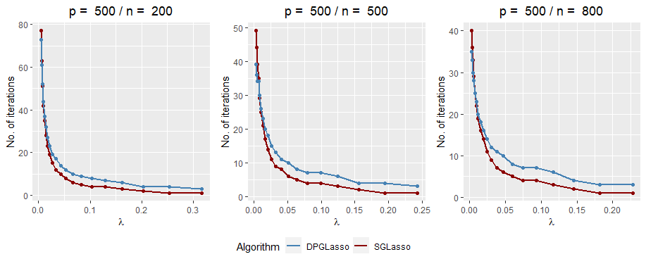
Figure 4: The number of iterations for path-wise S-GLasso and DP-GLasso with warm-start.

D.2 S-GLasso diagnostic

As discussed in Table 1 in the main text, S-GLasso, unlike GLasso, solves the primal problem, is monotone, and maintains positive definiteness over the iterations. In this section, we use the data generation method described in Example 1 of Mazumder and Hastie (2011, Appendix A.1.) to empirically demonstrate these properties. Specifically, we generate data from a Gaussian distribution with $n=2,p=5$, and run S-GLasso with a carefully chosen warm start for which GLasso fails to converge. The results are displayed in Figure 5. The left plot displays iterations over the objective function (criterion) difference, i.e. $f(\Theta^{(k+1)})-f(\Theta^{(k)})$, where $f(\Theta)=-\log\det(\mbox{\boldmath$\Theta$})+\mbox{tr}(\mathbf{S}\mbox{\boldmath$\Theta$})+\lambda\|\mbox{\boldmath$\Theta$}\|_{1},$. If the optimization is not monotonic then we expect multiple 0 crossings over the iterations, which is not the case for S-GLasso. The middle plot shows that S-GLasso maintains the positive definiteness over the iterations, since the minimum eigenvalue of the working precision matrix is always positive. Finally, the right figure shows that S-GLasso optimizes the primal problem.

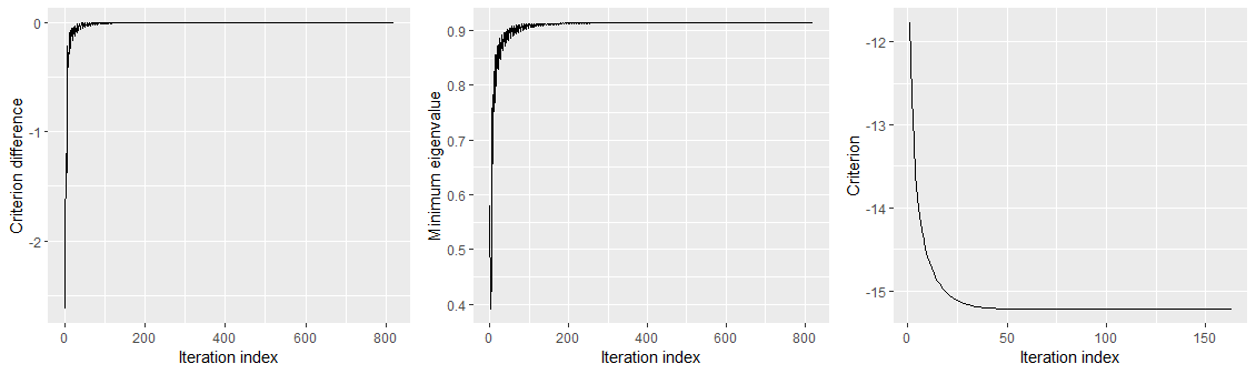
Figure 5: S-GLasso diagnostic plot.

D.3 Computational Time

In this section, we utilize R package microbenchmark to report the computational time of S-GLasso for $p=\{10,50,100,200,400,800,1000\}$ and $n=400$. The data is generated using function huge.generator() from the huge package such that the population precision matrices has approximately 70% of the entries equal to zero. For each $p$, we choose $\lambda_{p}=0.5*\lambda^{p}_{max}$, where $\lambda^{p}_{\max}$ is the maximum of the non-diagonal elements of $\mathbf{S}_{p}$ and corresponds to the smallest value for which $\mbox{\boldmath$\Theta$}_{p}$ is a diagonal matrix.

All simulations are run on AMD Ryzen 9 5900X with 12-core processor. As can be seen in Figure 6, S-GLasso requires on average 50 second computational time for $p=1000$.

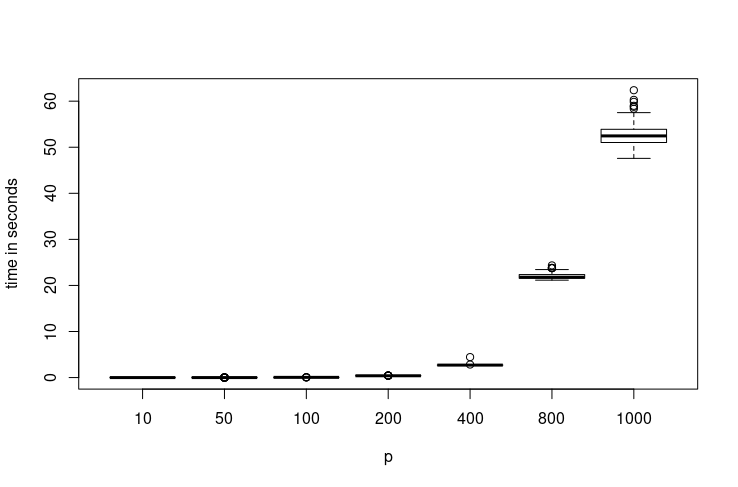
Figure 6: Computational time of S-GLasso in seconds.

D.4 The auto-regressive process

Similar to Mazumder and Hastie (2011), we consider data generated from the AR(2) process with a tri-diagonal precision matrix such that the diagonal elements are equal to 1, the first and second sub and super-diagonal elements are equal to 0.5 and 0.25, respectively.

• $p=200,\,n\in\{50,200,500\}$

• $p=500,\,n\in\{200,500,800\}$

• $p=800,\,n\in\{500,800,1000\}$

• $p=1000,\,n\in\{500,1000,1500\}$

Similar to (Mazumder and Hastie, 2011), we implement S-GLasso and DP-GLasso for every combination of $(n,p)$ on a grid of twenty linearly spaced $\lambda$ values, where $\lambda_{i}=0.8^{i}(0.9\lambda_{\max})\,,i=1,\dots,20$, using a cold start initialization , i.e. $\mbox{\boldmath$\Theta$}^{(0)}=(\mbox{diag}(\mathbf{S})+\lambda\boldsymbol{I})^{-1}$. Here, $\lambda_{\max}$ is the maximum of the non-diagonal elements of $\mathbf{S}$ and corresponds to the smallest value for which $\Theta$ is a diagonal matrix.

In Table 3 and Figure 7, we report results only for $p=500$ and $p=1000$, which are consistent with results in Experiment 1 of the manuscript.

Table 3: AUC score for S-GLasso and DP-GLasso

p	n	S-GLasso	DP-GLasso
500	200	0.91066	0.91057
	500	0.69306	0.69205
	800	0.67128	0.66827
1000	500	0.52142	0.52142
	1000	0.59177	0.59175
	1500	0.63596	0.63595

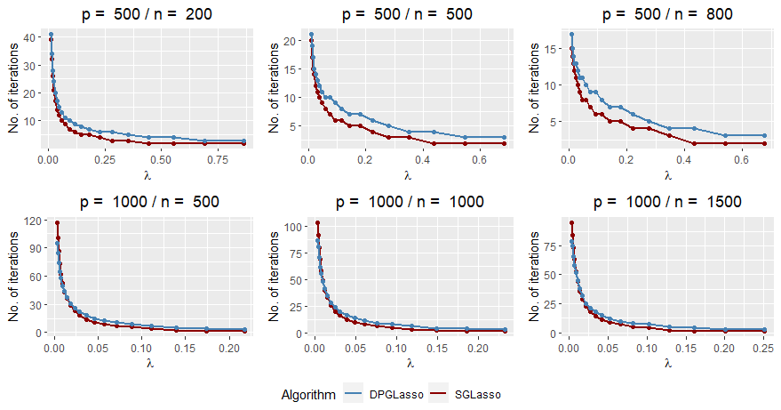
Figure 7: Number of iterations for S-GLasso and DP-GLasso.

Appendix E Micro-array example

In this section, we use a data-set in Alon et al. (1999) and analyzed in Mazumder and Hastie (2011) and Mazumder and Hastie (2012). Data, obtained from the R package colonCA, contains $n=62$ tissue samples of Affymetrix Oligonucleotide array ($p=2000$ genes). Similar to Mazumder and Hastie (2012), we use the exact covariance thresholding to reduce data to $p=716$, which is the largest component in the graph, where the edge $E_{ij}\neq 0$ if and only if $|\mathbf{S}_{ij}|>\tau$, where $\tau$ is the threshold.

Figure 8 reports the average number of iterations for a grid of fifteen $\lambda$ values.

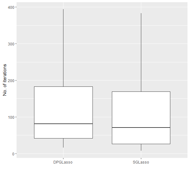
Figure 8: Average number of iterations of S-GLasso and DP-GLasso for micro-array example.

References

- Alon et al. (1999) Alon, Uri, Naama Barkai, Daniel A. Notterman, Kenneth W. Gish, Suzanne E. Ybarra, Douglas Michael Mach, and Arnold J. Levine (1999), “Broad patterns of gene expression revealed by clustering analysis of tumor and normal colon tissues probed by oligonucleotide arrays.” Proceedings of the National Academy of Sciences of the United States of America, 96 12, 6745–50.
- Banerjee et al. (2008) Banerjee, O., L. E. Ghaoui, and A. d’Aspermont (2008), “Model selection through sparse maximum likelihood estimation for multivariate gaussian or binary data.” Journal of Machine Learning Research, 9, 485–516.
- Friedman et al. (2008) Friedman, J., T. Hastie, and R. Tibshirani (2008), “Sparse inverse covariance estimation with the graphical lasso.” Biostatistics, 9, 432–441.
- Horn and Johnson (2012) Horn, R.A. and C.R. Johnson (2012), Matrix Analysis. Cambridge University Press.
- Mazumder and Hastie (2012) Mazumder, Rahul and Trevor Hastie (2012), “Exact covariance thresholding into connected components for large-scale graphical lasso.” Journal of Machine Learning Research, 13, 781–794.
- Mazumder and Hastie (2011) Mazumder, Rahul and Trevor J. Hastie (2011), “The graphical lasso: New insights and alternatives.” Electronic journal of statistics, 6, 2125–2149.
- Tseng (2001) Tseng, Paul (2001), “Convergence of a block coordinate descent method for nondifferentiable minimization.” Journal of Optimization Theory and Applications, 109, 475–494.
- Wang (2014) Wang, Hao (2014), “Coordinate descent algorithm for covariance graphical lasso.” Statistics and Computing, 24, 521–529.