Sim2Real in Reconstructive Spectroscopy:
Deep Learning with Augmented Device-Informed Data Simulation

Abstract

This work proposes a deep learning (DL)-based framework, namely Sim2Real, for spectral signal reconstruction in reconstructive spectroscopy, focusing on efficient data sampling and fast inference time. The work focuses on the challenge of reconstructing real-world spectral signals under the extreme setting where only device-informed simulated data are available for training. Such device-informed simulated data are much easier to collect than real-world data but exhibit large distribution shifts from their real-world counterparts. To leverage such simulated data effectively, a hierarchical data augmentation strategy is introduced to mitigate the adverse effects of this domain shift, and a corresponding neural network for the spectral signal reconstruction with our augmented data is designed. Experiments using a real dataset measured from our spectrometer device demonstrate that Sim2Real achieves significant speed-up during the inference while attaining on-par performance with the state-of-the-art optimization-based methods.

1 Introduction

Optical spectroscopy is a versatile technique for various scientific, industrial, and consumer applications. Recently, computational spectroscopy using reconstructive algorithms [1, 2, 3, 4, 5, 6, 7, 8] has been rapidly developed owing to its potential to enable a miniaturized spectrometer [9, 10]. A spectrometer encodes optical spectral information spatially or temporally and then measures the encoded information using a series of photodetectors. The transformation between the input signal $\bm{x}$ and the photo-detector readout $\bm{y}$ in a spectrometer design can be either linear or nonlinear. However, a linear design is typically preferred. An example of a nonlinear encoding is observed in Fourier-Transform infrared (FTIR) spectrometers, which produce an auto-correlation of the input through a variable time-delay interferometer. For a linear system, $\bm{x}$ and $\bm{y}$ can be represented using column vectors while the mapping is represented by a responsivity matrix $\bm{R}$ such that $\bm{y}=\bm{Rx}$. For example, a monochromator spatially disperses different spectral components with a block-diagonal $\bm{R}$ matrix. In a reconstructive spectrometer, $\bm{R}$ is generally much more complex. Each photo-detector’s readout depends on all instead of a few spectral components. While the complex structure of $\bm{R}$ means a lot of computational resources are generally required to recover the spectrum $\bm{x}$ from the photo-detector readouts $\bm{y}$, it also opens up new opportunities. These include the ability to tailor $\bm{R}$ to encode the spectral information directly to parameters of interest in the application, such as the spectral peak positions and the relative intensities between the peaks; the ability to increase the accuracy of spectral reconstruction by focusing on the most important spectral information even when $\bm{y}$’s dimension is much smaller than $\bm{x}$’s[11]; and the ability to miniaturize the spectrometer.

A wealth of research has been conducted to increase spectral reconstruction’s efficiency and accuracy. The approaches can generally be categorized as optimization-based or data-driven. The optimization based approaches formulate the inverse problem into a convex optimization problem in terms of the signal to be reconstructed. To deal with non-uniqueness of the solution, different types of regularizations (e.g., nonnegativity, sparsity, and smoothness) have been considered [12, 13, 1]. The effectiveness of these optimization-based techniques often hinges on the precise adjustment of regularization parameters and hyperparameters, a task that can be challenging [14]. Moreover, optimization-based approaches based on iterative procedures can be energy and computationally expensive for critical applications such as Internet-of-Things or time-sensitive tasks. Despite the challenges, miniaturized spectrometers based on these spectral-reconstruction techniques have reported good performance. For example, we recently developed a chip-scale spectrometer concept by integrating 16 semiconductor photo-detectors, each with a different spectral response [13]. We designed the photo-detectors using nanostructured materials to minimize the dependence on the incident angle of light and thus eliminated the need for any external optical components. The entire spectrometer, sans the electronic readout circuitry, is only a few microns thick. As the photodetector’s response was broadband, the device was able to recover basic spectral information, including the positions and relative intensities of peaks across the entire visible spectrum. The accuracy of reconstructing a multi-peak spectrum were 0.97% (RMS error) for locating the peak locations, comparable to a monochromator with twice the number of detectors. Enabled by the rich interaction between different spectral components in each photo-detector, we also showed that only seven detectors were sufficient for input signals with up to three peaks and had relatively smooth spectra.

In comparison, deep learning-based data-driven approaches [8, 15, 16] showed the potential to address the challenges of an optimization-based approach. First, deep overparametrized networks trained by gradient descent methods tend to enforce the regularization implicitly[17], avoiding the need to adjust regularization parameters. Second, while training neural networks can be computationally expensive, reconstructing a new measurement during inference requires only a single forward pass through the network. In contrast, optimization-based approaches can be costly in terms of energy and computing resources during inference. Various data-driven methods of reconstructive spectroscopy have been developed, including utilizing a simple, fully connected network on a plasmonic spectral encoder on the device[8], minimizing potential noise before the reconstruction process on a colloidal quantum dot spectrometer[16], and a specifically tailored residual convolutional neural network aiming to improve the reconstruction performance[15].

A significant challenge with the current deep learning methodologies is their dependence on extensive volumes of real, precisely annotated training data to achieve optimal performance[8, 14]. The process of gathering such real, labeled data for spectrometer reconstruction is both costly and time-intensive in a practical setting. Additionally, the actual labeled data pairs collected often contain considerable noise, which, when used to train deep learning models, may result in poor performance during testing.

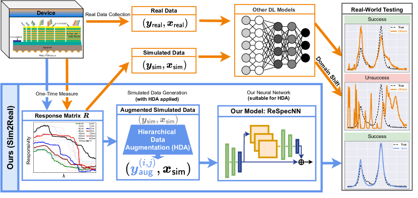
Figure 1: The diagram of our proof-of-concept Sim2Real framework in the reconstructive spectroscopy. The orange arrows denote existing methods, which require collecting and training on real-world data. The blue box and arrows denote our contribution Sim2Real that effectively bridges the domain gap between simulated and real-world data. See Section 2 for details.

In this work, we introduce a method to tackle these challenges in deep learning-based approaches for spectral reconstruction. As illustrated in Figure 1, we propose a Sim2Real framework in which we train the deep learning models solely based on experimentally simulated datasets and then deploy the model on a real dataset. Our method contains two key components:

• Hierarchical Data Augmentation (HDA): To mitigate the domain gap between simulated and real data, we introduce a data augmentation technique to perturb both the response matrix $\bm{R}$ and the encoded signal. Training the model with these data improves its robustness.

• ReSpecNN: In line with this, we developed a new lightweight network architecture specifically designed for the Sim2Real framework applied to spectral reconstruction problem with HDA, thereby further improving the model’s robustness.

Unlike conventional methods, marked by orange arrows in Figure 1, which require collecting and training on real-world data, our strategy eliminates the need for extensive real-world data collection, only requiring a single measurement of the response matrix $\bm{R}$. Moreover, by utilizing our augmented simulated training data, we effectively close the domain gap between simulated and real data, leading to high-quality spectral reconstruction during testing on real data.

The rest of the paper is organized as follows. In Section 2, we introduce the mathematical formulation of spectral reconstruction problem while identify limitations of existing method. In Section 3, we present our main contributions and discuss how they address the limitations of the existing method. In Section 4, we validate the performance of our proposed method on real-world data by comparing with state-of-the-art method and discuss the implications.

2 Problem formulation and existing Methods

In this section, we introduce the mathematical formulations of the spectrum reconstruction problem. We also identify the challenges and limitations of existing optimization and deep learning method.

2.1 Spectral Reconstruction Problem

For spectrometer signal reconstruction, the encoded signal vector $\bm{y}=(y_{1},\dots,y_{K})\in\mathbb{R}^{K}_{+}$ is the output produced by the spectrometer given the signal of interest $\bm{x}$ as input, and is modeled mathematically as:

$$y_{i} \textstyle=\int_{a}^{b}\bm{x}(\lambda)R_{i}(\lambda)\,d\lambda+\epsilon_{i}$$ (1)

$$\textstyle\approx\sum_{j=1}^{\ell}\bm{x}(\lambda_{j})R_{i}(\lambda_{j})\Delta\lambda+\epsilon_{i},\,\,\,\mbox{ for }i=1,\ldots,K,$$ (2)

where Equation 2 is the discrete approximation of the model. Here, we denote the spectral signal of interest at wavelength $\lambda$ by $\bm{x}(\lambda)\in\mathbb{R}_{+}$, where $\lambda$ belongs to some predetermined wavelength range of interest $[a,b]$. The signal is encoded, i.e., measured, by $K$ distinct spectral encoders with various responsivity at different wavelengths as shown in Figure 1. We denote $R_{i}(\lambda)$ as the the relative spectral power density of the $i$-th spectral encoder and $\epsilon_{i}$, the error of the $i$-th encoder, where $i\in\{1,\dots,K\}$. The error term, $\epsilon_{i}$, is a random quantity whose dependency on $\bm{x}$ is not assumed to be known.

As shown in Equation 2, sampling wavelengths $\{\lambda_{1},\dots,\lambda_{\ell}\}$ results in the equally spaced discretization of $[a,b]$ with a spectral resolution $(b-a)/\ell$. Stacking up the relative spectral power density for each encoder give us the response matrix $\bm{R}:=\begin{bmatrix}R_{ij}\end{bmatrix}_{i=1,\,j=1}^{K,\,\ell}\in\mathbb{R}^{K\times\ell}$ where $\bm{R}_{ij}:=R_{i}(\lambda_{j})$. As such, the discretization relationship between $\bm{y}$ and $\bm{x}$ could be expressed through $\bm{R}$ in a cleaner form:

$$\bm{y}=\bm{R}\bm{x}+\bm{\epsilon},\quad\mbox{ where }\bm{\epsilon}=[\epsilon_{1},\cdots,\epsilon_{K}]^{\top}$$ (3)

As such, our goal is to recover $\bm{x}$ from observed $\bm{y}$ and $\bm{R}$ under the setting where the number of encoders $K$ is much smaller than the number of sampled wavelengths $\ell$. In another word, the system in Equation 3 is highly under-determined with non-unique solutions.

2.2 Optimization Based Approaches and Limitations

Note that given the response matrix $\bm{R}$, the reconstruction problem in (3) can be approached using (non-negative) least squares as discussed in the introduction. Due to the ill-posedness of the problem, explicit regularization techniques are used to ensure unique solutions with desirable additional structures. Within optimization-based methods, the least-squares (LS) estimate $\hat{\bm{x}}\in\mathrm{argmin}_{\bm{x}}\|\bm{y}-\bm{Rx}\|_{2}^{2}$ fails to consider the signal’s nonnegativity, often leading to suboptimal solutions [18]. This issue can be addressed by employing nonnegative least squares (NNLS) [1]. To deal with underdetermined system, regularization strategies like $\ell_{1}$-norm, $\ell_{2}$-norm, or total-variation (TV) norm regularization have also been proven effective[12, 13].

However, solving these optimization problems can be time and memory consuming and their performance is sensitive to the choice of the regularization hyperparameter, so that they are often too expensive to deploy on chip-scaled devices.

2.3 Deep Learning Methods and Challenges

Recently, deep learning based approaches gained their popularity, due to their modelling flexibility and fast inference speed. However, a major bottleneck for effectively leveraging deep neural network models is gathering a large amount of real spectral data pairs $(\bm{y}_{\textsf{real}},\bm{x}_{\textsf{real}})$, a task that is both expensive and time-consuming in reconstructive spectroscopy.

Therefore, based on the problem formulation in Equation 3, previous approaches have focused on using the response matrix $\bm{R}$ to produce simulated spectral data pairs $(\bm{y}_{\textsf{sim}},\bm{x}_{\textsf{sim}})$, aiming to mimic the distribution of real data obtained in laboratory settings. However, we observe that models trained on such simulated data exhibit an undesirable phenomenon known as “domain gap”, resulting in poor performance on real data; see Figure 1. Later in Section 3, we delve into this issue and detail our approach to bridging the domain gap. For reader’s convenience, we first review previous approaches in detail.

Training on Simulated Data.

In practice, the simulated spectral signals $\bm{x}_{\textsf{sim}}$ can be viewed as the sum of Lorentzian distribution functions [15, 13]. Given the response matrix $\bm{R}$, a simulated spectral signal $\bm{x}_{\textsf{sim}}$ and its corresponding encoded signal $\bm{y}_{\textsf{sim}}$ can be generated as follows:

1. Generate $M$ single peak Lorentzian distribution functions independently with various standard deviations.

2. Sum and then normalize the heights of those Lorentzian curves within range $[0,1]$. We denote the result distribution as $\bm{x}_{\textsf{sim}}$.

3. Multiply $\bm{x}_{\textsf{sim}}$ with the response matrix $\bm{R}$ to produce the encoded signal $\bm{y}_{\textsf{sim}}=\bm{R}\bm{x}_{\textsf{sim}}$.

Specifically, in the first step, each (Lorentzian) peak is characterized by three parameters: the mean $\mu$, the width constant $\gamma$, and the intensity constant $I$. The parameters corresponds to the peak location, spectral width, and intensity magnitude, respectively. Each parameter is sampled i.i.d uniformly from a set of ranges to be chosen to match the specific characteristics of the spectrometer device. For our device, the ranges are $\mu\in[0,205]$, $\gamma\in[15,20]$ and $I\in[0.25,1]$ respectively.

Challenges in Deploying Trained Models on Real Data.

Equation (3) is a simplified model of the actual spectroscopy system. As such, the procedure in the previous section for generating simulated spectral signals $\bm{x}_{\textsf{sim}}$ and their corresponding encoded signals $\bm{y}_{\textsf{sim}}$ may produce distributions that differs from the distribution of real encoded signals $\bm{y}_{\textsf{real}}$. This may be attributed to the circuit design in reality may introduce diverse types of unknown noise into the system resulting in this distributional difference between real and simulated data. When applying machine learning algorithms, this difference, or “domain gap”, could cause degraded performance.

We illustrate this in Figure 2, where we train a model exclusively on simulated which can successfully reconstruct spectrum given simulated data as input. However, the model’s performance degrades significantly on real-world data, even when the real-world and simulated data appear visually similar. Detailed empirical evidences are discussed in Section 4.4.

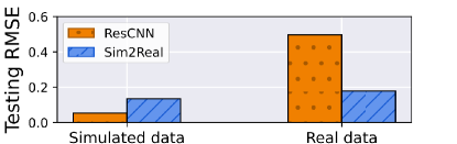
Figure 2: The testing RMSE on the simulated and real data[13] for ResCNN [15] and our proposed model ReSpecNN. Both models followed the Sim2Real training setting, that is, trained solely on simulated data. Our model further incorporated the hierarchical data augmentation during training, while ResCNN does not.

2.4 Domain Gap between “Sim” and “‘Real”

The challenges of “domain gap” are common for deep learning based approaches. The “domain gap” issue was first observed in transfer learning[19], where a model trained on a large source dataset is fine-tuned on a smaller, more specific dataset. To mitigate the performance degradation due to domain gaps between source and targeted datasets, many techniques have been proposed including domain adaptation[20, 21, 22], meta-learning[23], and few-shot learning[24, 25]. These techniques have been shown to be effective for reducing or closing the domain gap in various fields including computer vision[26, 27] and natural language processing[28, 29, 30].

However, in the context of spectroscopy reconstruction, those proposed method falls short to solve the domain gap for the following two reasons. First, we do not assume access to any data from the target distribution. Existing methods still require a certain amount of data from the targeted domain for fine-tuning, which is not applicable under our assumption. Second, most domain adaptation methods are designed for classification tasks, making them less directly applicable to our reconstructive spectroscopy problem, which is fundamentally a (non-negative) regression problem. While there are a few existing results focusing on practical regression problems [31, 32], they often deal with simpler regression scenarios rather than tackling the challenging inverse problem setting that we encounter.

Within the framework of deep learning for inverse problems, existing research primarily leverages the spatial structure of image signals for tasks like image reconstruction [33, 34, 35], whereas our work deals with one-dimensional spectral signals, presenting a different set of challenges and considerations. Therefore, a specialized method is required to tackle the domain shift encountered in the spectroscopy field. We now introduce the proposed Sim2Real framework in the following.

3 Our Sim2Real Method

In this section, we introduce the following Sim2Real framework to bridge the domain gap between the simulated encoded signal data and the data from real-world spectrometers. Our method tackles the domain gap by two key components: (i) hierarchical data augmentation for training data generation, and (ii) a new network architecture tailored for the spectrum reconstruction problem.

3.1 Hierarchical Data Augmentation

Although we measure the response matrix $\bm{R}$ in advance and consider it to be fixed and known, our hierarchical data augmentation strategy acknowledges the potential uncertainty in our measurement of $\bm{R}$ and the encoded signal vector $\bm{y}$ to improve model robustness and minimize the domain gap. For every pair of simulated training data $(\bm{y}\textsf{sim},\bm{x}\textsf{sim})$ introduced in Section 2.3, we systematically introduce noise as outlined in Algorithm 1.

Input:

    $\bm{x}_{\textsf{sim}}$: a simulated spectral signal from Section 2.3

    $\bm{R}$: the response matrix

    $p(\bm{R})$: the distribution of noise perturbation on $\bm{R}$

    $q(\bm{y^{(s)}_{\textsf{aug}}})$: the distribution of noise perturbation on $\bm{y^{(s)}_{\textsf{aug}}}$

    $S,T$: the augmentation numbers

Output:

    $(\bm{y}_{\textsf{aug}}^{(1,1)},\bm{x}_{\textsf{sim}}),\cdots,(\bm{y}^{(S,T)}_{\textsf{aug}},\bm{x}_{\textsf{sim}})$: training data pairs.

for $s=1,\cdots,S$ do

       Sample $\bm{\Delta}_{s}\sim p(\bm{R})$

       $\bm{R}_{s}=\bm{R}+\bm{\Delta}_{s}$

       $\bm{y}^{(s)}_{\textsf{aug}}=\bm{R}_{s}\bm{x}_{\textsf{sim}}$

       for $t=1,\cdots,T$ do

             Sample $\bm{\epsilon}_{t}\sim q(\bm{y^{(s)}_{\textsf{aug}}})$

             $\bm{y}^{(s,t)}_{\textsf{aug}}=\bm{y}^{(s)}_{\textsf{aug}}+\bm{\epsilon}_{t}$

            

       end for

      

end for

Algorithm 1 Hierarchical Data Augmentation (HDA)

To illustrate this process, we have provided a visualization in Figure 3, using an example of 3LED samples (number of peaks $M=3$) explained in detail below. Instead of simply multiplying response matrix $\bm{R}$, our hierarchical data augmentation extends each original simulated data sample $(\bm{y}_{\textsf{sim}},\bm{x}_{\textsf{sim}})$ to $S\times T$ augmented ones $(\bm{y}_{\textsf{aug}}^{(s,t)},\bm{x}_{\textsf{sim}})$ by adding different noises on the measured response matrix $\bm{R}$ (aquamarine green traces) and each intermediate augmented encoded signal (illustrated by $\bm{y}_{\textsf{aug}}^{(1)}$ only, light purple traces) respectively.

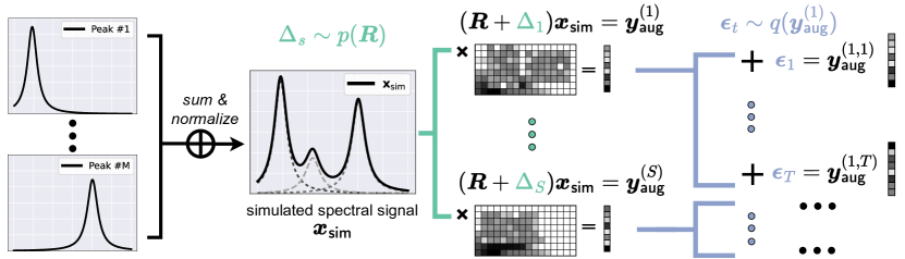
Figure 3: The diagram of the simulated data generation procedure and our proposed hierarchical data augmentation (HDA) scheme. Simulated spectral signal $\bm{x}_{\textsf{sim}}$ is generate through sum of Lorentzian distribution. For one given $\bm{x}_{\textsf{sim}}$, we generate many corresponding augmented encoded signals $\bm{y}^{(S,T)}_{\textsf{aug}}$ by adding noise $\Delta_{S}$ to $\bm{R}$ before multiplying with the spectral signal and adding noise $\bm{\epsilon}_{T}$ afterwards. The two noise distributions could be chosen flexibly. This HDA process is summarized in detail by Algorithm 1

To perturb the response matrix $\bm{R}$, we simply add Gaussian noise with zero mean and variance related to entries of $\bm{R}$. That is, for each noisy perturbation matrix $\bm{\Delta}_{s}$ ($s=1,\cdots,S$), its $(i,j)^{th}$ entry is sampled i.i.d from the distribution $\mathcal{N}\left(0,\ \sigma^{2}_{ij}\right)$ with $\sigma_{ij}=\alpha\cdot R_{ij}$, where $\alpha$ is a hyperparameter controlling the intensity of perturbation on $\bm{R}$. For perturbing the encoded signal $\bm{y}$, we inject nonnegative noise $\bm{\epsilon}_{t}$ ($t=1,\cdots,T$). Here, each entry of $\bm{\epsilon}_{t}$ is sampled i.i.d from the Gaussian distribution and then passed through the $\textsf{ReLU}(z)=\max\{0,z\}$ operator to enforce non-negativity.

In the case above, we considered adding Gaussian noise to disrupt the data, which is simple yet effective in practice. However, should specific information about the noise be accessible under certain conditions, we can further refine both distributions $p(\bm{R})$ and $q(\bm{y}^{(s)}_{\textsf{aug}})$, for the noise sampled on the response matrix and the intermediate augmented encoded signal, respectively. As a result, for each ground truth spectrum input $\bm{x}_{\textsf{sim}}$, $S\times T$ many corresponding augmented encoded signal vector $\bm{y}_{\textsf{aug}}^{(\cdot,\cdot)}$ are generated. This also demonstrates the generalizability and flexibility of our data augmentation method. By incorporating structured noise into the device-informed simulated data generation, we term this process Hierarchical Data Augmentation (HDA).

3.2 Network Architecture: ReSpecNN

For training with augmented data generated by HDA, we propose a deep neural network architecture tailored for spectrometer signal reconstruction, hereinafter referred to as RecSpecNN. The architecture is visualized in Figure 4 and explained in detail below.

Our model consists of two fully-connected modules and a 1D convolutional module. The first fully-connected module (rec_fc) aims to construct each spectrum at a gross level. To avoid the possible overfitting at this stage, dropout layers are incorporated after each fully-connected layer. This fully-connected module is followed by a convolutional module with three 1D convolutional layers (Conv1d in PyTorch), each followed by a max-pooling layer and a ReLU activation, serving to extract the potential spatial features from each wavelength value.

Subsequently, another fully-connected module (rf_fc), consisting of fully connected layers and dropout layers mirroring the rec_fc module, is employed for the detailed reconstruction of finer spectral information. Furthermore, a residual connection links the initial output from rec_fc with the detailed output from rf_fc, to improve the quality of the final prediction without losing the key spectral features from the initial reconstruction. A sigmoid function is applied at the end to ensure the final output spectrum is smooth and continuous.

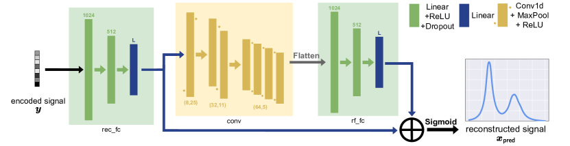
Figure 4: The architecture of our proposed neural network. ReSpecNN comprises two fully-connected modules (dubbed as rec_fc and rf_fc) and a three-layer convolutional neural network (dubbed as conv). Note that rec_fc and rf_fc have a residual connection. For each linear layer in fully-connected modules, the number above represents its output dimension, where $L$ denotes the number of input wavelengths. For each 1D convolutional layer, the tuple below specifies the number of filters and the kernel size.

4 Experimental Results

In this section, we illustrate the performance of our Sim2Real approach on real-world data by comparing both the test accuracy and the inference time with a state-of-the-art optimization-based method: NNLS with Total Variation regularization (NNLS-TV)[13].

4.1 Training Settings

To address the potential scaling difference between simulated and real inputs encoded signal values, the log-min-max normalization transformation is applied to convert the raw inputs $\bm{y}$ to $\widehat{\bm{y}}$ before fed into the neural network:

$$\widehat{\bm{y}}=\frac{\bm{z}-\min(\bm{z})}{\max(\bm{z})-\min(\bm{z})},\quad\mbox{where}\quad\bm{z}=\log\left(\bm{y}\right)$$ (4)

In the simulated data generation process, a batch size of $256$ is utilized. During the hierarchical data augmentation, we set $S=2$ and $T=4$. For the noise control parameters, we chose $\alpha=5\times 10^{-2}$ and $\sigma_{\epsilon}=1\times 10^{-5}$. During the training stage, we employed the MSELoss function in PyTorch as our training loss. The optimizer used was Adam with a learning rate of $3\times 10^{-4}$. To obtain the model for subsequent experiments, we performed $2\times 10^{4}$ iterations under the aforementioned hyperparameter settings.

4.2 Real-world Data Evaluation

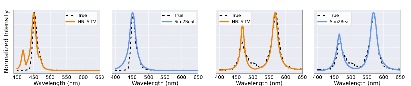
Figure 5: Visualization of the reconstructed spectral signals using real-world data (Left: a single-peak sample, Right: a double-peak sample) produced by NNLS-TV[13] and our Sim2Real approach. The corresponding ground-truth spectra are measured by a commercial spectrometer. Our Sim2Real approach achieves a comparable performance with NNLS-TV.

The real-world dataset is measured via a chip-scaled wearable spectrometer device [13] and compared with NNLS-TV method proposed in the same paper. To comprehensively compare our proposed Sim2Real deep learning framework and NNLS-TV[13], we evaluated their spectrum reconstruction results based on two key aspects: the accuracy of peak location and intensity. Relative peak position error, defined as

$$\text{Rel. error}\ \Delta\lambda/\lambda:=(\lambda_{\textsf{reconstructed}}-\lambda)/\lambda,$$

is measured for each reconstruction. Here, $\lambda_{\textsf{reconstructed}}$ denotes the wavelength position of the peak for the reconstructed spectral signal, while $\lambda$ corresponds to the position of the ground truth. To capture the overall performance, we also calculated the peak mean absolute error (MAE), defined as the average absolute value of the relative peak position error, across all reconstructed spectrum. Specific to multi-peaks spectrum, we also measured the relative intensity errors defined as

$$\text{Rel. error}\ \Delta I/I:=(I_{\textsf{reconstructed}}-I)/I,$$

where $I_{\textsf{reconstructed}}$ denotes the normalized peak intensity of the reconstructed spectral signal, while $I$ corresponds to the ground truth.

Figure 5 presents two spectrum reconstruction examples using our proposed deep neural network and the NNLS-TV[13] approach. When compared with the ground truths obtained by a commercial spectrometer, our approach exhibits a reliable performance on our miniature chip-scale spectrometer.

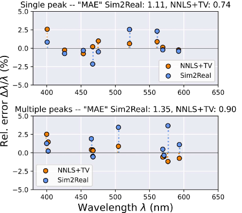
Figure 6: The relative peak position errors (vs. wavelength in nm) for single-peak real data (Top) and multiple-peak real data (Bottom). The plot title shows the mean absolute error (Abbrev. “MAE”) for each approach.

For peak position predictions, Figure 6 show that our approach yields a result comparable with NNLS-TV[13]. While offering a significantly faster inference speed (details to be discussed in next section), our model can still maintain the relative errors within -5 to 5 percent.

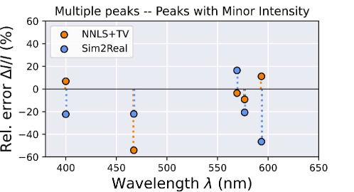
Figure 7: The relative intensity errors (vs. wavelength in nm) for the subset of “minor” peaks with relatively lower intensities.

Regarding the results for intensity ratios, which represent a more difficult challenge as illustrated in Figure 7, our method effectively constrained the maximum relative error in intensity to under 50 percent. In contrast, the NNLS-TV approach occasionally exhibits significant prediction errors.

4.3 Execution Time Analysis for Reconstruction Methods

Our miniature chip-scale spectrometers have been integrated into wearable health monitoring devices. In such scenarios, the inference time for reconstruction often emerges as a critical factor for achieving fast real-time health monitoring. Additionally, our pre-trained Sim2Real method offers the potential to conserve battery life, as it requires only one forward pass for inference, unlike NNLS-TV which requires sophisticated software or smart programs to iteratively solve it. Overall, prioritizing fast inference time is advantageous for real-time monitoring and extended battery life because of the low computational/energy costs involved in inference.

To demonstrate our superior inference time, we compared the execution time of our pre-trained model with the NNLS-TV solver using the real dataset[13]. The results in Table 1 show that our model significantly reduces inference time.

	NNLS+TV (MATLAB)	NNLS+TV (SciPy)	Ours (PyTorch)
Exec. Time (ms)	$10.634\pm 0.126$	$7.965\pm 0.230$	$\mathbf{1.134\pm 0.330}$

Table 1: The average execution time (per sample, in milliseconds) for the NNLS-TV[13] method and our proposed approach on the real dataset[13]. The NNLS-TV method[13] was originally implemented with the MATLAB solver lsqnonneg in the paper, and to ensure a fair comparison with our model implemented in PyTorch, we also implemented their method using scipy.optimize.nnls in SciPy.

4.4 Domain Shift in Reconstructive Spectroscopy

As previously discussed in Section 2.4, the domain shift usually exists between the device-informed simulated data $\bm{y}_{\textsf{sim}}$ and the real-world data $\bm{y}_{\textsf{real}}$. Many works only focus on improving the reconstruction accuracy within the datasets of the same distribution (i.e. training and testing exclusively on either simulated data or specific real-measured datasets) without attempting to bridge the domain gap between them. For instance, ResCNN[15] has been demonstrated to achieve excellent spectral reconstruction performance and maintain stable results even under some noisy conditions. It preprocessed the input data from $\bm{y}$ to $\widetilde{\bm{x}}:=\bm{R}^{\dagger}\bm{y}$ ($\bm{R}^{\dagger}$ is the pseudoinverse of $\bm{R}$) for improved results. However, ResCNN trained only on simulated data do not perform optimally when directly applied to real-world data[13].

Figure 2 illustrates a comparison of the root mean square error (RMSE) under the Sim2Real setting between the spectral signals reconstructed by ResCNN and our ReSpecNN, against the ground truths for both the device-informed simulated data and the real data collected from our spectrometer[13]. While ResCNN nearly perfectly fits the simulated data (with a lower RMSE), its performance on the real dataset[13] tends to drop significantly under the Sim2Real training setting, which confirm the domain shift phenomenon.

5 Conclusion and Discussion

In this paper, we introduce a new Sim2Real framework for spectral signal reconstruction in spectroscopy, focusing on the sampling efficiency and inference time. Throughout the training process, only a single measurement of the response matrix $\bm{R}$ for a particular spectrometer device is required, with all other training data being simulated or synthetically generated. To bridge the domain gap between the real-world data and the device-informed simulated data, our Sim2Real framework introduce the hierarchical data augmentation approach to train our deep learning model. Furthermore, our neural network, ReSpecNN, which is trained exclusively on augmented simulated data, is specifically designed for the reconstruction of real spectral signals. In our experiments, even with the simplest Gaussian noise augmentation, our Sim2Real method achieving a 10-fold speed-up during the inference compared to the state-of-the-art optimization-based solver NNLS-TV[13], while demonstrates on par performance in terms of the solution quality.

Moving forward, we aim to further improve the performance of our model across various scenarios. First, it would be interesting to explore improved noise patterns within our HDA process to further improve our model’s robustness, such as incorporating fast gradient sign noise used in the adversarial training of deep networks[36]. Furthermore, while our current focus is on scenarios without labelled real training data, it is possible that some limited labelled real data could be available in practical situations. In such cases, we could fine-tune our model using this data. However, the limited size of fine-tuning dataset poses a risk of overfitting. To mitigate this, one possible idea is to utilize the simulated training data for regularization during the fine-tuning phase, as outlined in the recent study [37].

Data Availability Statement

The testing spectral data and our experimental results are available at https://github.com/j1goblue/Rec_Spectrometer.

References

- [1] Cheng-Chun Chang and Heung-No Lee. On the estimation of target spectrum for filter-array based spectrometers. Optics Express, 16(2):1056–1061, 2008.
- [2] Umpei Kurokawa, Byung Il Choi, and Cheng Chun Chang. Filter-based miniature spectrometers: Spectrum reconstruction using adaptive regularization. IEEE Sensors Journal, 11:1556–1563, 2011.
- [3] Jie Bao and Moungi G Bawendi. A colloidal quantum dot spectrometer. Nature, 523(7558):67–70, 2015.
- [4] Zhu Wang and Zongfu Yu. Spectral analysis based on compressive sensing in nanophotonic structures. Optics Express, 22:25608, 10 2014.
- [5] Zhu Wang, Soongyu Yi, Ang Chen, Ming Zhou, Ting Shan Luk, Anthony James, John Nogan, Willard Ross, Graham Joe, Alireza Shahsafi, Ken Xingze Wang, Mikhail A. Kats, and Zongfu Yu. Single-shot on-chip spectral sensors based on photonic crystal slabs. Nature Communications, 10:1020, 12 2019.
- [6] Cheolsun Kim, Woong-Bi Lee, Soo Kyung Lee, Yong Tak Lee, and Heung-No Lee. Fabrication of 2d thin-film filter-array for compressive sensing spectroscopy. Optics and Lasers in Engineering, 115:53–58, 2019.
- [7] Tuba Sarwar, Srinivasa Cheekati, Kunook Chung, and Pei-Cheng Ku. On-chip optical spectrometer based on gan wavelength-selective nanostructural absorbers. Applied Physics Letters, 116:081103, 2 2020.
- [8] Calvin Brown, Artem Goncharov, Zachary S. Ballard, Mason Fordham, Ashley Clemens, Yunzhe Qiu, Yair Rivenson, and Aydogan Ozcan. Neural network-based on-chip spectroscopy using a scalable plasmonic encoder. ACS Nano, 15(4):6305–6315, 2021. PMID: 33543919.
- [9] Jiajun Meng, Jasper J. Cadusch, and Kenneth B. Crozier. Plasmonic mid-infrared filter array-detector array chemical classifier based on machine learning. ACS Photonics, 8(2):648–657, 2021.
- [10] Shang Zhang, Yuhan Dong, Hongyan Fu, Shao-Lun Huang, and Lin Zhang. A spectral reconstruction algorithm of miniature spectrometer based on sparse optimization and dictionary learning. Sensors, 18(2):644, Feb 2018.
- [11] Emmanuel J Candes, Justin K Romberg, and Terence Tao. Stable signal recovery from incomplete and inaccurate measurements. Communications on Pure and Applied Mathematics: A Journal Issued by the Courant Institute of Mathematical Sciences, 59(8):1207–1223, 2006.
- [12] Leonid I. Rudin, Stanley Osher, and Emad Fatemi. Nonlinear total variation based noise removal algorithms. Physica D: Nonlinear Phenomena, 60(1):259–268, 1992.
- [13] Tuba Sarwar, Can Yaras, Xiang Li, Qing Qu, and Pei-Cheng Ku. Miniaturizing a chip-scale spectrometer using local strain engineering and total-variation regularized reconstruction. Nano Letters, 22(20):8174–8180, 2022. PMID: 36223431.
- [14] Pengyu Li, Can Yaras, Tuba Sarwar, Pei-Cheng Ku, and Qing Qu. Accelerating deep learning in reconstructive spectroscopy using synthetic data. In CLEO 2023, page JTu2A.71. Optica Publishing Group, 2023.
- [15] Cheolsun Kim, Dongju Park, and Heung-No Lee. Compressive sensing spectroscopy using a residual convolutional neural network. Sensors, 20(3):594, Jan 2020.
- [16] Jinhui Zhang, Xueyu Zhu, and Jie Bao. Denoising autoencoder aided spectrum reconstruction for colloidal quantum dot spectrometers. IEEE sensors journal, 21(5):6450–6458, 2020.
- [17] Sanjeev Arora, Nadav Cohen, Wei Hu, and Yuping Luo. Implicit regularization in deep matrix factorization. Advances in Neural Information Processing Systems, 32, 2019.
- [18] Umpei Kurokawa, Byung Il Choi, and Cheng-Chun Chang. Filter-based miniature spectrometers: spectrum reconstruction using adaptive regularization. IEEE Sensors Journal, 11(7):1556–1563, 2010.
- [19] Sinno Jialin Pan and Qiang Yang. A survey on transfer learning. IEEE Transactions on knowledge and data engineering, 22(10):1345–1359, 2009.
- [20] Eric Tzeng, Judy Hoffman, Kate Saenko, and Trevor Darrell. Adversarial discriminative domain adaptation. In Proceedings of the IEEE conference on computer vision and pattern recognition, pages 7167–7176, 2017.
- [21] Yaroslav Ganin and Victor Lempitsky. Unsupervised domain adaptation by backpropagation. In International conference on machine learning, pages 1180–1189. PMLR, 2015.
- [22] Weichen Zhang, Wanli Ouyang, Wen Li, and Dong Xu. Collaborative and adversarial network for unsupervised domain adaptation. In Proceedings of the IEEE conference on computer vision and pattern recognition, pages 3801–3809, 2018.
- [23] Chelsea Finn, Pieter Abbeel, and Sergey Levine. Model-agnostic meta-learning for fast adaptation of deep networks. In International conference on machine learning, pages 1126–1135. PMLR, 2017.
- [24] Oriol Vinyals, Charles Blundell, Timothy Lillicrap, Daan Wierstra, et al. Matching networks for one shot learning. Advances in neural information processing systems, 29, 2016.
- [25] Jake Snell, Kevin Swersky, and Richard Zemel. Prototypical networks for few-shot learning. Advances in neural information processing systems, 30, 2017.
- [26] Ross Girshick, Jeff Donahue, Trevor Darrell, and Jitendra Malik. Rich feature hierarchies for accurate object detection and semantic segmentation. In Proceedings of the IEEE conference on computer vision and pattern recognition, pages 580–587, 2014.
- [27] Barret Zoph, Vijay Vasudevan, Jonathon Shlens, and Quoc V Le. Learning transferable architectures for scalable image recognition. In Proceedings of the IEEE conference on computer vision and pattern recognition, pages 8697–8710, 2018.
- [28] Andrew M Dai and Quoc V Le. Semi-supervised sequence learning. Advances in neural information processing systems, 28, 2015.
- [29] Jeremy Howard and Sebastian Ruder. Universal language model fine-tuning for text classification. arXiv preprint arXiv:1801.06146, 2018.
- [30] Jacob Devlin, Ming-Wei Chang, Kenton Lee, and Kristina Toutanova. Bert: Pre-training of deep bidirectional transformers for language understanding. arXiv preprint arXiv:1810.04805, 2018.
- [31] Xinyang Chen, Sinan Wang, Jianmin Wang, and Mingsheng Long. Representation subspace distance for domain adaptation regression. In ICML, pages 1749–1759, 2021.
- [32] Ismail Nejjar, Qin Wang, and Olga Fink. Dare-gram: Unsupervised domain adaptation regression by aligning inverse gram matrices. In Proceedings of the IEEE/CVF Conference on Computer Vision and Pattern Recognition, pages 11744–11754, 2023.
- [33] Chao Dong, Chen Change Loy, Kaiming He, and Xiaoou Tang. Image super-resolution using deep convolutional networks. IEEE transactions on pattern analysis and machine intelligence, 38(2):295–307, 2015.
- [34] Kuldeep Kulkarni, Suhas Lohit, Pavan Turaga, Ronan Kerviche, and Amit Ashok. Reconnet: Non-iterative reconstruction of images from compressively sensed measurements. In Proceedings of the IEEE conference on computer vision and pattern recognition, pages 449–458, 2016.
- [35] Gregory Ongie, Ajil Jalal, Christopher A Metzler, Richard G Baraniuk, Alexandros G Dimakis, and Rebecca Willett. Deep learning techniques for inverse problems in imaging. IEEE Journal on Selected Areas in Information Theory, 1(1):39–56, 2020.
- [36] Ian J Goodfellow, Jonathon Shlens, and Christian Szegedy. Explaining and harnessing adversarial examples. arXiv preprint arXiv:1412.6572, 2014.
- [37] Nataniel Ruiz, Yuanzhen Li, Varun Jampani, Yael Pritch, Michael Rubinstein, and Kfir Aberman. Dreambooth: Fine tuning text-to-image diffusion models for subject-driven generation. In Proceedings of the IEEE/CVF Conference on Computer Vision and Pattern Recognition, pages 22500–22510, 2023.