INVESTIGATION OF NON-EQUILIBRIUM IONIZATION PLASMA DURING A GIANT FLARE OF UX ARIETIS TRIGGERED WITH MAXI AND OBSERVED WITH NICER

Abstract

We detected a giant X-ray flare from the RS-CVn type binary star UX Ari using MAXI on 2020 August 17 and started a series of NICER observations 89 minutes later. For a week, the entire duration of the flare was covered with 32 snapshot observations including the rising phase. The X-ray luminosity reached 2$\times$10³³ erg s^-1 and the entire energy release was $\sim 10^{38}$ erg in the 0.5–8.0 keV band. X-ray spectra characterized by continuum emission with lines of Fe XXV He$\alpha$ and Fe XXVI Ly$\alpha$ were obtained. We found that the temperature peaks before that of the flux, which suggests that the period of plasma formation in the magnetic flare loop was captured. Using the continuum information (temperature, flux, and their delay time), we estimated the flare loop size to be $\sim 3\times 10^{11}$ cm and the peak electron density to be $\sim 4\times 10^{10}$ cm^-3. Furthermore, using the line ratio of Fe XXV and Fe XXVI, we investigated any potential indications of deviation from collisional ionization equilibrium (CIE). The X-ray spectra were consistent with CIE plasma throughout the flare, but the possibility of an ionizing plasma away from CIE was not rejected in the flux rising phase.

1 Introduction

Solar and stellar flares are considered to be caused by the same physical mechanisms but with different scales (e.g.; Fletcher et al. 2011; Benz & Güdel 2010). The accumulated magnetic energy is impulsively released through magnetic reconnection and plasma instability (Priest & Forbes, 2002; Shibata & Magara, 2011). In the standard model for the eruptive flares, known as the CSHKP model (Carmichael, 1964; Sturrock, 1966; Hirayama, 1974; Kopp & Pneuman, 1976), the released energy is partially converted into the kinetic energy of charged particles at the reconnection site, which then bombard the flare loop top and cause an impulsive increase in temperature. The particles move downward along the loop and collide with the dense chromosphere. The evaporated matter fills the loop, causing the flux to peak. After the initial rise, the temperature decreases conductively and radiatively.

Because of this dynamic process, it is expected and often observed that the temperature peak precedes the flux peak (e.g.; Maggio et al. 2000; Pillitteri et al. 2022; Stelzer et al. 2022). This rising phase is the time when physical constraints of flares can be obtained independently from and more stringently than the decay phase. Reale (2007) proposed a model to describe the behavior of X-ray light curves during flares and derived analytical formulae relating observables with physical properties of flares and applied them to observations. In X-ray observations of stellar flares, the observables are often limited to values obtained from the continuum emission (such as temperature and volume emission measure; hereafter called “continuum observables”), but those from the line emission (“line observables”) will carry independent information about the flare dynamics. However, this has been hampered by the lack of spectral resolution or photon statistics (Favata et al., 2000; Maggio et al., 2000; Stelzer et al., 2002).

Of particular interest are line ratios that deviate from collisional ionization equilibrium (CIE), as it is an expected consequence of the dynamic nature of flares, thus providing new keys to understanding flare physics (Imada et al., 2011; Reale & Orlando, 2008; Bradshaw & Mason, 2003). There are some observational claims (Kawate et al., 2016; Imada, 2021) of non-equilibrium ionization (NEI) plasma in solar flares, but such observations are limited despite the continuous and intensive observations of the Sun. The largest obstacle is the short duration of NEI conditions expected to last only for $\mathcal{O}(10^{2}~{}\mathrm{s})$.

Stellar flare observations could be more advantageous. The electron temperature is $\sim 10$ times larger than the Sun during flares (Feldman et al., 1995), which makes the equilibrium time scales longer for the same electron density, as more charged ions dominate the population and the ionization/recombination rate coefficient decreases. In order to exploit this advantage, we need X-ray observations from the rising phase of stellar flares using a telescope with a large collecting area and the capability to distinguish major lines of different charges.

We break through this limitation by combining two X-ray instruments onboard the International Space Station (ISS): the Monitor of All-sky X-ray Image (MAXI; Matsuoka et al. 2009) and the Neutron star Interior Composition Explorer (NICER; Gendreau et al. 2016). MAXI updates all-sky X-ray images every 92 minutes, which has led to 167 detections of stellar flares from 30 objects since 2009. NICER has an ability to conduct fast maneuvers and collect photons with a larger effective area and a better spectral resolution than MAXI.

We have developed two systems, in which MAXI detects transient events and NICER responds in the shortest achievable time. One is OHMAN (Orbiting High-energy Monitor Alert Network), in which the triggering from MAXI to NICER is automated within the ISS. OHMAN has been in operation since 2023 but is effective only for very bright sources. The other is MANGA (MAXI And NICER Ground Alert) since 2017, in which a human decision is inserted based on the MAXI data downlinked to the ground. MANGA still makes human-triggered observations faster than any previous approaches. In our study, we use MANGA for stellar flare observations (e.g., Iwakiri et al. 2018; Sasaki et al. 2021).

We present here the result of the MANGA observation made with the shortest response time to date for stellar flares. We detected a giant flare from UX Ari with MAXI and initiated NICER observations well before the flux peak. UX Ari is an RS-CVn type binary system consisting of a K0 IV and G5 V star with a 6.4 day orbital period (Hummel et al., 2017). The source is known to cause occasional flares in X-rays (Franciosini et al., 2001; Tsuboi et al., 2016; Güdel et al., 1999; Tsuru et al., 1989). The peak flare luminosity of the present data reaches 2$\times$10³³ erg s^-1 in the 0.5–8.0 keV band, which is $\sim$10 times larger than any flares observed with X-ray pointing observations of this source. The goal of this study is to examine the plasma development throughout the flare and investigate any hints of the off-CIE plasma using the X-ray spectra. Throughout the paper, we use AtomDB (Smith et al., 2001; Foster et al., 2017) for plasma calculations. The quoted uncertainties are for 90% statistical error.

2 Observations

2.1 Instrument

NICER is a payload onboard the ISS equipped with an X-ray Timing Instrument (XTI). XTI is an assembly of 56 sets of X-ray concentrators (Okajima et al., 2016) and silicon drift detectors (Prigozhin et al., 2016), of which 52 are in routine use. The energy range is 0.2–12.0 keV. The effective area and the energy resolution in FWHM at 6 keV are $\sim$ 600 cm² and 137 eV, respectively.

NICER is useful for wide astrophysical applications. In particular, the operational flexibility, the large effective area, and the fast detector readout allow spectroscopic observations of eruptive events uncompromised by limitations of photon statistics and detector dynamic range. These features make NICER particularly well suited for stellar flare observations (Namekata et al., 2020; Sasaki et al., 2021; Hamaguchi et al., 2023).

2.2 Observation and data reduction

We captured a flux increase of UX Ari based on the MAXI Nova-Alert system (Negoro et al., 2016) recorded on 2020 August 17 11:51:54 (UT). Using the MANGA system, the first NICER observation was executed 89 minutes later. NICER continued observations for a week (ObsIDs: 3100380101–3100380106) until the X-ray count rate returned to the pre-flare level. NICER visited the source 32 times, which we refer to as snapshot 0 to 31. The on-source exposure ranged from 101 to 1286 s with an average of 752 s and the photon counts ranged from $2.2\times 10^{4}$ to $2.0\times 10^{6}$ with an average of $4.0\times 10^{5}$ counts. Thanks to the large effective area of NICER, it can accumulate sufficient counts even with short exposure times.

We applied level 2 processing using the nicerl2 tasks to incorporate the latest calibration and event screening and produced level 3 products using the nicerl3 tasks in HEASoft version 6.32.1 (HEASARC, 2014). The level 3 products include the telescope and detector response files, binned source spectrum, and background spectrum based on the SCORPEON model, which we generated and used for each snapshot.

3 Analysis

3.1 Light curve and spectra

Fig. 1 (a) shows the X-ray light curve of the data set. Snapshot 0 captures the rising part of the flare, 1 captures the flux peak, and the rest shows the decaying part. There is a slight re-brightening during 14–16 and 26–29. The peak luminosity and the e-folding time of the NICER light curve are $2\times 10^{33}$ erg s^-1 and $2.4\times 10^{4}$ s, respectively, deriving the total released energy in 0.5–12 keV to be $\sim 10^{38}$ erg.

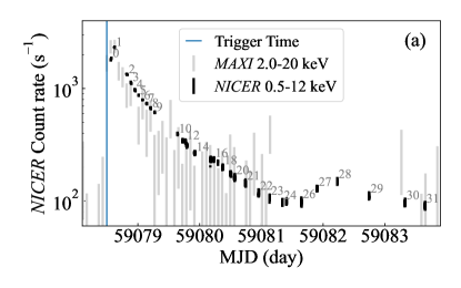
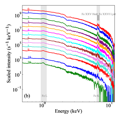
Figure 1: (a) NICER (black) and MAXI (grey) light curves. MAXI count rate is scaled to match with NICER. The labels 0–31 are given for each NICER snapshot. (b) NICER X-ray spectra with different colors for different snapshots. The intensity of each spectrum is offset incrementally by 0.5 dex for clarity.

Fig. 1 (b) shows the X-ray spectra for the first ten snapshots (0–9) and two selected later ones(19 and 29). The spectra are characterized by continuum emission with lines. The most conspicuous feature is found at the Fe K band, in which Fe XXV He$\alpha$ and Fe XXVI Ly$\alpha$ emission lines are identified at 6.7 and 7.0 keV.

The development of the line pair traces the decreasing plasma temperature. The intensity ratio of Fe XXVI Ly$\alpha$ against Fe XXV He$\alpha$ monotonically decreases with time, suggesting that the Fe²⁵⁺ (H-like) population is taken over by Fe²⁴⁺ (He-like) in the charge state distribution. At the end of the flare (snapshot 29), the Fe XXV He$\alpha$ feature almost disappears and the Fe L features at $\sim$1 keV increases, suggesting that Fe²⁴⁺ is taken over by Fe²³⁺ (Li-like) and less charged ions.

3.2 Spectral modeling

3.2.1 Phenomenological model

We first tried a phenomenological model to explore the characteristics of the data set. We used the first eight snapshots with sufficient statistics for fitting in the energy range of interest (5–10 keV). We assessed the level of the persistent emission using the last part of the datasets (snapshots 24–31 except for 27–29 with a possible rebrightening) when the flare seemed settled. Its contribution to the first part of the flare (snapshots 0–7) is smaller than a fraction of $\sim$ 0.1 in the energy band of interest. We do not use time-sliced spectra within each snapshot, as we found that they exhibit no significant change between the former and the latter halves.

The model is composed of two components: a Bremsstrahlung model for the continuum and Gaussian models for the lines. A total of nine Gaussian lines are added: three for Fe XXVI Lyman series (Ly$\alpha$, Ly$\beta$, and Ly$\gamma$), three for Fe XXV $n=2\rightarrow 1$ series (He$\alpha$, He$\beta$, and He$\gamma$), and He$\alpha$ lines of other He-like ions of Cr XXIII, Mn XXIV, and Ni XXVII.

The fitting was conducted simultaneously for the two components. The free parameters for the Bremsstrahlung component are the electron temperature ($T_{\mathrm{e}}$) and the emission measure ($EM$). For the Gaussian components, we fitted their normalization individually and the energy shift collectively within $\pm$1% around the center. The line widths were fixed to null. For the Lyman series, the energy averaged between ($n$p) ${}^{2}P_{1/2}$ $\rightarrow$ (1s) ${}^{2}S_{1/2}$ and ($n$p) ${}^{2}P_{3/2}$ $\rightarrow$ (1s) ${}^{2}S_{1/2}$ weighted by their statistical weights is used as the line center, where $n\in\left\{2,3,4\right\}$. For the He series, the energy for ($n$p1s) ${}^{1}P_{1}$ $\rightarrow$ (1s)² ${}^{1}S_{0}$ is used among several fine-structure lines that spread over $<$1% of the line energy for Cr, Mn, Fe, and Ni. All fits were statistically acceptable. Fig. 2 depicts the results of the fitting.

3.2.2 Physical models

We next applied three physical models: CIE, ionizing, and recombining plasmas. They are respectively implemented as apec, nei, and rnei models in the xspec spectral fitting package (Arnaud, 1996). The latter two are off-CIE plasmas in opposite directions. The ionizing plasma model assumes the initial condition in which ions are neutral and electrons have a temperature higher than the neutral ions. The degree of Coulomb relaxation is parameterized by the ionization parameter $\tau=\int_{0}^{t}n_{\mathrm{e}}(t^{\prime})dt^{\prime}$, in which $n_{\mathrm{e}}(t^{\prime})$ is the time-varying electron density and $t$ is the time from the initial state. The recombining plasma model assumes the opposite initial condition that ions are ionized for a given initial temperature and electrons have a lower temperature. Their relaxation is also parameterized by $\tau$. Recombining plasma conditions might be observed if the cooling via thermal conduction occurs more rapidly than charge state equilibration after impulsive heating of the plasma.

The free parameters for CIE plasma model are the electron temperature ($T_{\mathrm{e}}$), abundance ($Z_{\odot}$) relative to the cosmic value (Anders & Grevesse, 1989), and emission measure ($EM$). For the ionizing and recombining plasma, the ionization parameter $\tau$ is also added. The initial temperature of the recombining plasma was fixed to the value obtained in the phenomenological fitting of snapshot 0. All fits were statistically acceptable. The results of the fitting are illustrated in Fig. 2.

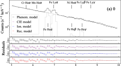
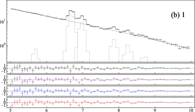
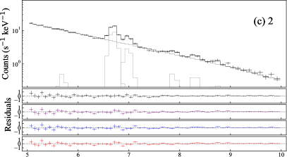
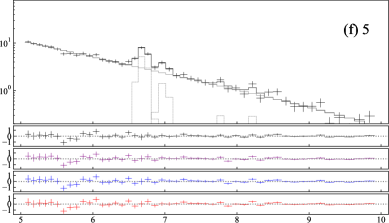
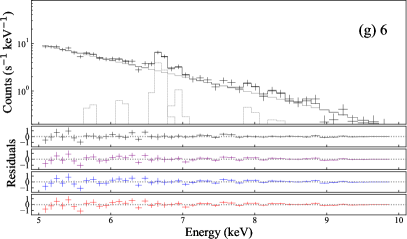
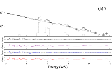
Figure 2: Spectra and best-fit phenomenological model (upper-most panel) and the residuals of the fit (other panels) for the phenomenological model (black), CIE plasma model (purple), ionizing plasma model (blue), and recombining plasma model (red) for snapshots 0–7.

4 Discussion

4.1 Continuum observables

We first explored the continuum observables following the previous work by Reale (2007). We used the result of the phenomenological spectral fitting (§ 3.2.1). Fig. 3 (a and b) shows the development of the best-fit values of $T_{\mathrm{e}}$ and $EM$. The peak of $EM$ (snapshot 1) is delayed from that of $T_{\mathrm{e}}$ (snapshot 0) in time for $\sim 5\times 10^{3}$ s, as in Fig. 1 of Reale (2007). We assume that the density peak coincides with the $EM$ peak in snapshot 1. It is notable that $T_{\mathrm{e}}$ and $EM$ do not monotonically decrease. They stagnate or increase around snapshots 3–4, which may suggest repeated heating.

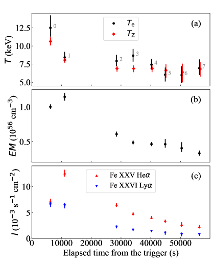
Figure 3: Evolution of best-fit values for $T_{\mathrm{e}}$, $T_{\mathrm{Z}}$, $EM$, and line intensities of Fe XXV He$\alpha$ and Fe XXVI Ly$\alpha$ in the phenomenological model. The discrepancy between the electron temperature $T_{\mathrm{e}}$ and the ionization temperature $T_{\mathrm{Z}}$ suggests an off-CIE plasma.

Based on the estimated delay time ($\Delta t_{\mathrm{lag}}\sim 5\times 10^{3}$ s), we can infer the flare loop half-length $L$ and the peak density $n_{\rm{M}}$ by using Eqn. (13) and (9) in Reale (2007):

$$\left(\frac{L}{10^{9}~{}\mathrm{cm}}\right)=2.5\frac{\psi}{\ln{\psi}}\left(\frac{T_{0}}{10^{7}~{}\mathrm{K}}\right)^{\frac{1}{2}}\left(\frac{\Delta t_{\mathrm{lag}}}{10^{3}~{}\mathrm{s}}\right)$$ (1)

$$\left(\frac{n_{\mathrm{M}}}{10^{10}~{}\mathrm{cm^{-3}}}\right)=13\left(\frac{T_{\mathrm{M}}}{10^{7}~{}\mathrm{K}}\right)^{2}\left(\frac{L}{10^{9}~{}\mathrm{cm}}\right)^{-1}$$ (2)

where $\psi=\frac{T_{0}}{T_{\mathrm{M}}}$ is the ratio of the maximum temperature $T_{0}$ and temperature at the density peak $T_{\mathrm{M}}$, and $\Delta t_{\mathrm{lag}}$ is the time lag between $T_{\mathrm{e}}$ and $EM$. These relations are derived from the assumption that the density reaches its maximum when the radiative cooling rate equals the conductive cooling rate. $L$ is estimated to be $\sim 3\times 10^{11}$ cm ($\sim$4 $R_{\odot}$), which is much larger than the typical value for solar flares ($\sim 10^{9}$ cm) and even comparable to the scales of the binary system; the radii of UX Ari Aa and Ab are 5.6 $R_{\odot}$ and 1.6 $R_{\odot}$, respectively, and the binary separation is $\sim 0.1$ AU$\sim 20~{}R_{\odot}$ (Hummel et al., 2017). The density maximum gives a fairly similar value $n_{\mathrm{M}}\sim 4\times 10^{10}$ cm^-3 to solar coronal plasma density in flaring regions (Aschwanden & Benz, 1997). Since the plasma is confined by the magnetic flux tube, the magnetic field strength ($B$) can be estimated from the pressure balance. Assuming the plasma to be an ideal gas, $B>\sqrt{16\pi n_{\mathrm{M}}T_{\mathrm{M}}}\sim 200$ G. By additionally using the measured $EM$ value, the aspect ratio between the loop length and the loop cross section radius is estimated to be $\sim$ 0.6. These values are of the same order as those in other giant stellar flares (Favata & Schmitt, 1999; Maggio et al., 2000; Franciosini et al., 2001; Reale et al., 2004; Reale, 2007; Sasaki et al., 2021; Pillitteri et al., 2022).

4.2 Line observables

4.2.1 Phenomenological model

We next examined the line observables. Using the phenomenological spectral fitting (§ 3.2.1), the development of the line intensities of Fe XXV He$\alpha$ and Fe XXVI Ly$\alpha$ is shown in Fig. 3 (c). Their intensities are well-constrained thanks to the photon-rich spectra. In order to examine any deviation from CIE, the line ratio of Fe Ly$\alpha$ and He$\alpha$ was derived for each snapshot. The Ly$\alpha$ against He$\alpha$ is larger in snapshot 1 than snapshot 2 despite a similar $T_{\mathrm{e}}$ value. Here, we used the line ratio of the same elements to avoid systematics caused by elemental abundance.

We calculated the expected line ratio as a function of $T_{\mathrm{e}}$ for CIE, ionizing, and recombining plasmas (Fig. 4). The starting condition for the ionizing/recombining plasma is that all Fe ions are neutral/ionized. The line intensities were extracted from the synthesized X-ray spectra calculated for $\tau=10^{12}-10^{13}$ cm^-3 s with geometrical spacing. The Ly$\alpha$ and He$\alpha$ line complexes that are unresolved with NICER were combined.

Based on the calculated results, we plotted the observed results. Snapshot 0 significantly deviates from CIE in the ionizing direction. It approaches CIE for snapshot 1, but deviates again in the ionizing direction for snapshot 3. The later snapshots are consistent with CIE within uncertainties. The ionization temperature ($T_{\mathrm{Z}}$) derived from the line ratio assuming CIE is compared with the electron temperature from the continuum emission ($T_{\mathrm{e}}$) in Fig. 3 (a). The two temperatures are in disagreement in snapshots 1 and 3.

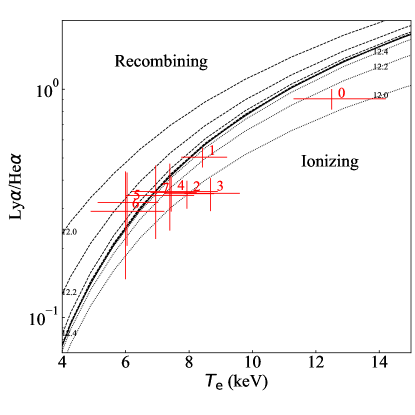
Figure 4: Line ratio of Fe XXVI Ly$\alpha$ over Fe XXV He$\alpha$. Different cases are shown in different line styles: CIE (solid), recombining (dashed), and ionizing (dotted) plasmas of varying $\log_{10}{\tau}$ (cm^-3 s) from 12.0 to 13.0 with a step of 0.2. Data points are plotted with red error bars and the snapshot number.

4.2.2 Physical model

Fig. 5 shows the development of the best-fit values of the parameters of the three physical models. All the parameters change similarly for the three models, suggesting that the off-CIE features in the spectra are insignificant. The best-fit $\tau$ values for the two off-CIE plasma models are $\gtrsim 1\times 10^{13}$ cm^-3 s, which is sufficiently large to reach equilibrium.

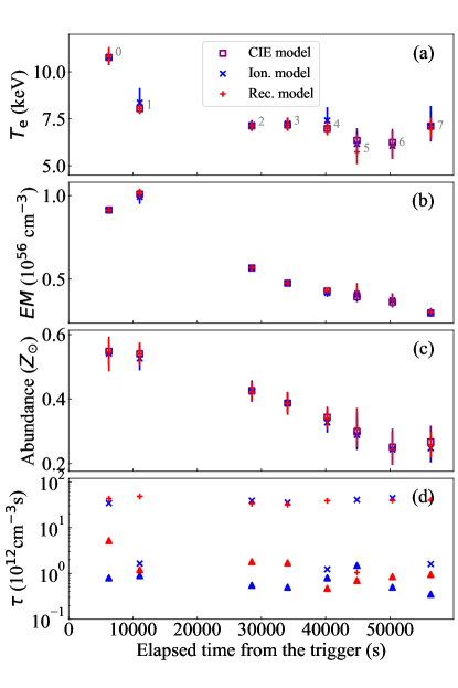
Figure 5: Evolution of best-fit values for $T_{\mathrm{e}}$, $EM$, and abundance of the three physical models, and $\tau$ in the physical models. For $\tau$, lower limits are illustrated as triangle symbols.

The phenomenological model suggests an off-CIE plasma in the ionizing direction in snapshots 0 and 3 (Fig. 4), whereas the physical ionizing plasma model suggests CIE condition. This discrepancy arises from the different assessments of $T_{\mathrm{e}}$. In the former, $T_{\mathrm{e}}=12.5\pm^{1.7}_{1.2}$ and $8.7\pm^{0.9}_{0.8}$ keV for snapshots 0 and 3. In the latter, $T_{\mathrm{e}}=10.8\pm^{0.5}_{0.4}$ and $~{}7.2\pm^{0.3}_{0.4}$ keV. The physical models determine $T_{\mathrm{e}}$ using not only continuum information but also line information. Because the energy range of the current dataset does not cover the expected cut-off of the Bremsstrahlung continuum, the $T_{\mathrm{e}}$ constraint by the continuum emission alone is loose. As a result, two fitting solutions of high $T_{\mathrm{e}}$/low $\tau$ or low $T_{\mathrm{e}}$/high $\tau$ are allowed.

In order to investigate the coupling nature of the two parameters, we made a contour plot in the ($T_{\mathrm{e}}$, $\tau$) space for snapshots 0 and 3 using the ionizing plasma model (Fig. 6). The contours indicate that either solution is acceptable: CIE plasma of $\tau\gtrsim 5\times 10^{12}$ cm^-3 s with $T_{\mathrm{e}}$ more stringently constrained than $\tau$ (thus vertically long part of the contours) and the ionizing plasma of $\tau\sim 1\times 10^{12}$ cm^-3 s with $\tau$ more stringently constrained than $T_{\mathrm{e}}$ (thus horizontally long part of the contours). The best-fit parameter pair of the physical ionizing plasma model resides in the former, whereas that of the phenomenological model resides in the latter. We conclude that the present spectra do not allow us to distinguish between these two possibilities.

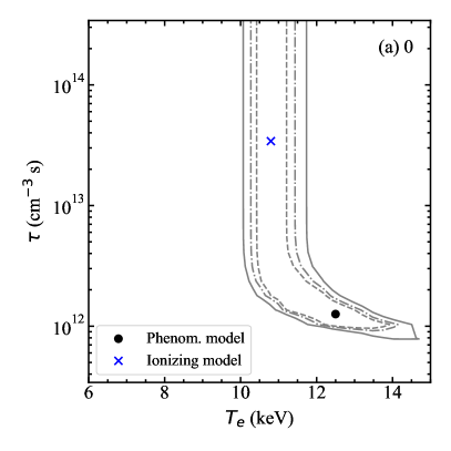
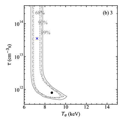
Figure 6: Contour plots of confidence intervals on ($T_{\mathrm{e}}$, $\tau$) for snapshots 0 and 3. Dashed, dashed-and-dotted, and solid lines correspond to 68%, 90%, and 99%. The best-fit values for the phenomenological model and the physical ionizing plasma model are shown with markers. The $\tau$ of the phenomenological model is derived from Fig. 4.

The development of the light curve favors CIE solution. Assume that there is no continued heating in the rising phase and the density increases linearly in time as

$$n(t)=n_{0}(t-t_{\mathrm{start}}),$$ (3)

where $t_{\mathrm{start}}$ is the flare start time that is assumed to be the MAXI trigger time (Fig. 1 a). The normalization $n_{0}$ satisfies $n(t_{1})=n_{\mathrm{M}}=4\times 10^{10}$ cm^-3, in which $t_{1}$ is the time of the snapshot 1. Then, the ionization parameter at snapshot 0 ($t_{0}$) is $\tau_{0}=\int_{t_{\mathrm{start}}}^{t_{0}}n(t)dt\sim 10^{14}$ cm^-3 s, which is large enough to reach an ionization equilibrium.

5 Conclusion

Based on the MAXI trigger, we observed a giant X-ray flare from UX Ari using NICER. Thanks to the rapid trigger response made possible by the MANGA system, we successfully captured the rising phase of the flux. Photon-rich spectra were obtained throughout the flare covered by 32 snapshot observations with NICER.

Using the continuum information (temperature, flux, and their peak delays), we constrained the flare loop size $\sim 3\times 10^{11}$ cm and the peak electron density $\sim 4\times 10^{10}$ cm^-3, which are consistent with other giant stellar flares. Furthermore, using the line information (ratio of the Fe XXV He$\alpha$ and Fe XXVI Ly$\alpha$ lines), we examined any hints of off-CIE plasma. We fitted the 5–10 keV spectra with a phenomenological model and three physical models of CIE, ionizing, and recombining plasmas. The X-ray spectra are consistent with CIE plasma throughout the flare, but the ionizing plasma away from CIE also explains the spectra in the flux rising phase.

The present study demonstrated the possibility of conducting X-ray spectroscopy studies of the rising part of stellar flares without relying on luck to capture one during long exposures. In the near future, we expect that two improvements can be made. One is the X-ray observation beyond 10 keV using NuSTAR (Vievering, 2019) to constrain the electron temperature $T_{\mathrm{e}}$ more precisely. The other is high-resolution spectroscopy using XRISM. The microcalorimeter will resolve the line complex with more constraining power for off-CIE signatures.

References

- Anders & Grevesse (1989) Anders, E., & Grevesse, N. 1989, Geochimica et Cosmochimica acta, 53, 197
- Arnaud (1996) Arnaud, K. A. 1996, in Astronomical Data Analysis Software and Systems V, ed. G. Jacoby & J. Barnes, Vol. 101, 17, doi: 1996ASPC..101…17A
- Aschwanden & Benz (1997) Aschwanden, M. J., & Benz, A. O. 1997, The Astrophysical Journal, 480, 825
- Benz & Güdel (2010) Benz, A. O., & Güdel, M. 2010, ARA&A, 48, 241, doi: 10.1146/annurev-astro-082708-101757
- Bradshaw & Mason (2003) Bradshaw, S. J., & Mason, H. E. 2003, A&A, 401, 699, doi: 10/bmx79b
- Carmichael (1964) Carmichael, H. 1964, in NASA Special Publication, Vol. 50, 451
- Favata et al. (2000) Favata, F., Reale, F., Micela, G., et al. 2000, A&A, 353, 987, doi: 10.48550/arXiv.astro-ph/9909491
- Favata & Schmitt (1999) Favata, F., & Schmitt, J. H. M. M. 1999, Spectroscopic Analysis of a Super-Hot Giant Flare Observed on Algol by BeppoSAX on 30 August 1997, arXiv, doi: 10.48550/arXiv.astro-ph/9909041
- Feldman et al. (1995) Feldman, U., Laming, J., & Doschek, G. 1995, The Astrophysical Journal, 451, L79
- Fletcher et al. (2011) Fletcher, L., Dennis, B. R., Hudson, H. S., et al. 2011, Space Sci. Rev., 159, 19, doi: 10.1007/s11214-010-9701-8
- Foster et al. (2017) Foster, A. R., Smith, R. K., & Brickhouse, N. S. 2017, Atomic Processes in Plasmas (APiP 2016), 1811, 190005, doi: 10/grmqvp
- Franciosini et al. (2001) Franciosini, E., Pallavicini, R., & Tagliaferri, G. 2001, A&A, 375, 196, doi: 10.1051/0004-6361:20010830
- Gabriel (1972) Gabriel, A. 1972, Monthly Notices of the Royal astronomical society, 160, 99
- Gendreau et al. (2016) Gendreau, K. C., Arzoumanian, Z., Adkins, P. W., et al. 2016, Proc. of SPIE, 9905, 99051H, doi: 10/gg664x
- Güdel et al. (1999) Güdel, M., Linsky, J. L., Brown, A., & Nagase, F. 1999, ApJ, 511, 405, doi: 10.1086/306651
- Hamaguchi et al. (2023) Hamaguchi, K., Reep, J. W., Airapetian, V., et al. 2023, ApJ, 944, 163, doi: 10.3847/1538-4357/acae8b
- HEASARC (2014) HEASARC. 2014, HEAsoft: Unified Release of FTOOLS and XANADU, Astrophysics Source Code Library, record ascl:1408.004. http://ascl.net/1408.004
- Hirayama (1974) Hirayama, T. 1974, Sol. Phys., 34, 323, doi: 10.1007/BF00153671
- Hummel et al. (2017) Hummel, C. A., Monnier, J. D., Roettenbacher, R. M., et al. 2017, The Astrophysical Journal, 844, 115
- Imada (2021) Imada, S. 2021, ApJL, 914, L28, doi: 10.3847/2041-8213/ac063c
- Imada et al. (2011) Imada, S., Murakami, I., Watanabe, T., Hara, H., & Shimizu, T. 2011, ApJ, 742, 70, doi: 10.1088/0004-637X/742/2/70
- Iwakiri et al. (2018) Iwakiri, W., Sasaki, R., Gendreau, K., et al. 2018, The Astronomer’s Telegram, 12248, 1
- Kawate et al. (2016) Kawate, T., Keenan, F. P., & Jess, D. B. 2016, The Astrophysical Journal, 826, 3, doi: 10/gg6658
- Kopp & Pneuman (1976) Kopp, R. A., & Pneuman, G. W. 1976, Sol. Phys., 50, 85, doi: 10.1007/BF00206193
- Maggio et al. (2000) Maggio, A., Pallavicini, R., Reale, F., & Tagliaferri, G. 2000, A&A, 356, 627
- Matsuoka et al. (2009) Matsuoka, M., Kawasaki, K., Ueno, S., et al. 2009, PASJ, 61, 999, doi: 10.1093/pasj/61.5.999
- Namekata et al. (2020) Namekata, K., Maehara, H., Sasaki, R., et al. 2020, Publications of the Astronomical Society of Japan, 72, 68, doi: 10/grmqxd
- Negoro et al. (2016) Negoro, H., Kohama, M., Serino, M., et al. 2016, Publications of the Astronomical Society of Japan, 68, S1
- Okajima et al. (2016) Okajima, T., Soong, Y., Balsamo, E. R., et al. 2016, Proc. of SPIE, 9905, 99054X, doi: 10/grmqzk
- Pillitteri et al. (2022) Pillitteri, I., Argiroffi, C., Maggio, A., et al. 2022, A&A, 666, A198, doi: 10.1051/0004-6361/202244268
- Priest & Forbes (2002) Priest, E. R., & Forbes, T. G. 2002, A&A Rev., 10, 313, doi: 10.1007/s001590100013
- Prigozhin et al. (2016) Prigozhin, G., Gendreau, K., Doty, J. P., et al. 2016, Proc. of SPIE, 9905, 99051I, doi: 10/gg664z
- Reale (2007) Reale, F. 2007, A&A, 471, 271, doi: 10.1051/0004-6361:20077223
- Reale et al. (2004) Reale, F., Güdel, M., Peres, G., & Audard, M. 2004, Astronomy & Astrophysics, 416, 733
- Reale & Orlando (2008) Reale, F., & Orlando, S. 2008, ApJ, 684, 715, doi: 10.1086/590338
- Sasaki et al. (2021) Sasaki, R., Tsuboi, Y., Iwakiri, W., et al. 2021, ApJ, 910, 25, doi: 10.3847/1538-4357/abde38
- Shibata & Magara (2011) Shibata, K., & Magara, T. 2011, Living Reviews in Solar Physics, 8, 6, doi: 10.12942/lrsp-2011-6
- Smith et al. (2001) Smith, R. K., Brickhouse, N. S., Liedahl, D. A., & Raymond, J. C. 2001, Spectroscopic Challenges of Photoionized Plasmas, 247, 161
- Stelzer et al. (2022) Stelzer, B., Caramazza, M., Raetz, S., Argiroffi, C., & Coffaro, M. 2022, A&A, 667, L9, doi: 10.1051/0004-6361/202244642
- Stelzer et al. (2002) Stelzer, B., Burwitz, V., Audard, M., et al. 2002, A&A, 392, 585, doi: 10.1051/0004-6361:20021188
- Sturrock (1966) Sturrock, P. A. 1966, Nature, 211, 695, doi: 10.1038/211695a0
- Tsuboi et al. (2016) Tsuboi, Y., Yamazaki, K., Sugawara, Y., et al. 2016, PASJ, 68, 90, doi: 10/gg667s
- Tsuru et al. (1989) Tsuru, T., Makishima, K., Ohashi, T., et al. 1989, PASJ, 41, 679
- Vievering (2019) Vievering, J. T. 2019, PhD thesis, University of Minnesota