A fast low-rank inversion algorithm of dielectric matrix in GW approximation

Abstract

The dielectric response function and its inverse are crucial physical quantities in materials science. We propose an accurate and efficient strategy to invert the dielectric function matrix. The GW approximation, a powerful approach to accurately describe many-body excited states, is taken as an application to demonstrate accuracy and efficiency. We incorporate the interpolative separable density fitting (ISDF) algorithm with Sherman–Morrison–Woodbury (SMW) formula to accelerate the inversion process by exploiting low-rank properties of dielectric function in plane-wave GW calculations. Our ISDF–SMW strategy produces accurate quasiparticle energies with $O(N_{\mathrm{r}}N_{\mathrm{e}}^{2})$ computational cost ($N_{\mathrm{e}}$ is the number of electrons and $N_{\mathrm{r}}=100$–$1000N_{\mathrm{e}}$ is the number of grid points) with negligible small error of $0.03$ eV for both complex molecules and solids. This new strategy for inverting the dielectric matrix can be $50\times$ faster than the current state-of-the-art implementation in BerkeleyGW, resulting in two orders of magnitude speedup for total GW calculations.

School of Mathematical Sciences, Fudan University, Shanghai 200433, China

Hefei National Research Center for Physical Sciences at the Microscale, University of Science and Technology of China, Hefei, Anhui 230026, China

School of Data Science, University of Science and Technology of China, Hefei, Anhui 230026, China

MOE Key Laboratory for Mathematical Foundations and Applications of Digital Technology, University of Science and Technology of China, Hefei, Anhui 230026, China

School of Data Science, Fudan University, Shanghai 200433, China

MOE Key Laboratory for Computational Physical Sciences, Fudan University, Shanghai 200433, China

E-mail: zbzhou21@m.fudan.edu.cn; myshao@fudan.edu.cn; whuustc@ustc.edu.cn

1 Introduction

The dielectric functions and polarizability functions are important physical quantities in condensed matter physics and computational chemistry. Experimentally, the dielectric function can be utilized to simulate optical properties observed in experiments, such as absorption, reflection, and energy loss [1]. On a theoretical level, many ground-state-based calculations concerning excited-state necessitate the utilization of the dielectric response function and polarizability function [2, 3]. The polarizability function is closely related to the dielectric function, and its inversion through the Dyson equation and differential relation. Computing the inverse of dielectric function matrix becomes one of the most important steps in excited-state calculations.

There are two primary approaches to invert the dielectric matrix. The conventional method involves explicitly constructing the irreducible polarizability function, then the dielectric matrix, and finally inverting it. The alternative approach involves obtaining the polarizability function through the Sternheimer equation and subsequently deriving the dielectric function [4]. Since the latter approach cannot explicitly obtain the dielectric function, in most applications the first approach is preferred. However, the dielectric function, $\epsilon(\mathbf{r},\mathbf{r}^{\prime})$, becomes an $N_{\mathrm{r}}\times N_{\mathrm{r}}$ matrix after discretization especially for plane waves. Consequently, the conventional approach requires quartic time in terms of the number of electrons $N_{\mathrm{e}}$ to construct the dielectric function initially, followed by another cubic scaling time with a huge prefactor (around $10^{9}$) to invert the dielectric function matrix. This approach becomes very costly for large-scale calculations. Since the inversion process is indispensable in most excited-state calculations, the complexity of excited-state calculations becomes prohibitively expensive for large systems.

The GW method is an excited-state method rooted in many-body Green’s function theory. It has become the gold standard for one-particle excitation energy calculations due to its balance between efficiency and accuracy [5, 6, 7]. Over the past decades, it has proven to be a powerful tool for describing one-particle excitations in various systems, including molecular [8, 9, 10] and solid-state materials [11, 12]. Researchers have applied the GW method to investigate material science hotspots such as low-dimensional nanostructures and surfaces [13]. Several methods and algorithms have been developed based on the GW method, including G₀W₀ [6], GW$\Gamma$ [14], scGW [15], among others. G₀W₀, as a variation of the GW method, simplifies the computation by setting both the Green’s function and the screened Coulomb interaction to be one-shot, resulting in lower time complexity compared to other alternatives.

Although G₀W₀ calculation makes a concession to the accuracy, it is still too expensive for many applications. As an excited-state method, G₀W₀ calculation also requires inverting the dielectric function matrix. This step introduces a quartic term and a cubic term with ultra high factor in the complexity of the G₀W₀ calculation. BerkeleyGW, which was in the finalist of the ACM Gordon Bell Prize of $2020$ [16] and is regarded the state-of-art implementation of the GW calculation, also mentioned the difficulty introduced by the huge prefactor. For instance, it takes $25.08$ seconds and $162$ MB RAM for the DFT calculation with Quantum ESPRESSO [17] to calculate all bands of Si₃₂ with a single processor, while the static COHSEX G₀W₀ calculation with BerkeleyGW costs $24454.35$ seconds and $2519$ MB RAM.

To reduce computational cost and memory usage, several low-scaling algorithms have been proposed. One such algorithm is the tensor hypercontraction (THC) algorithm [18], known as the interpolative separable density fitting (ISDF) algorithm [19, 20]. The ISDF algorithm compresses orbital pair functions through a low-rank approximation, significantly accelerating multi-center integral calculations in quantum chemistry. Moreover, the ISDF algorithm has been applied to develop an accurate and efficient cubic scaling GW calculation strategy for both molecular and solid systems, using atomic orbitals [21] and a plane-wave basis set [22]. However, these implementations still require explicitly inverting the dielectric function matrix, leaving the huge prefactor unresolved. To address this issue, Liu et al. provide an approach to compute the inverse using the Sherman–Morrison–Woodbury (SMW) formula [10]. Although the prefactor when inverting the matrix is significantly reduced, this process is only applicable to small systems that contain tens of atoms because of its $\mathcal{O}({N_{\mathrm{e}}^{6}})$ time complexity and $\mathcal{O}({N_{\mathrm{e}}^{4}})$ space complexity.

In this work, we present an accurate and effective cubic scaling algorithm by combing the ISDF low-rank approximation and the SMW formula to invert the dielectric function matrix $\epsilon(\mathbf{r},\mathbf{r}^{\prime})$ with a small prefactor and low memory usage. We also apply this fast low-rank inversion algorithm to the G₀W₀ calculations as an application to excited-state calculations, illustrating the accuracy and efficiency of our algorithm. Table 1 summarizes the notation of important variables and operators in this work.

2 Result and discussion

2.1 Theoretical framework of fast inversion of dielectric matrix and its application in GW calculation

The dielectric function and polarizability functions are significant physical quantity in computational chemistry and condensed matter physics, both experimentally and theoretically. The polarizability function is closely related to the inverse of dielectric function. Inverting the dielectric function matrix becomes one of the most important steps in excited-state calculations. The conventional process to construct the inverse of dielectric matrix is first constructing dielectric matrix with quartic time complexity and cubic space complexity, and then inverting it with cubic time complexity but a huge prefactor.

We provide a cubic scaling method to invert the dielectric matrix accurately and efficiently with quadratic space complexity and a modest prefactor. We use the ISDF algorithm to generate polarizability operator and dielectric matrix with low-rank properties, so that the SMW formula can be adopted to invert the matrix. To eventually achieve cubic scaling, we apply Cauchy integral to the coupling part of the dielectric matrix. A detailed description of our fast low-rank inversion algorithm can be found in Section 3.

The GW method is a well-developed method to calculate the excited-state energies. The framework of GW method introduces self-energies to go beyond the mean-field approximation in DFT calculation and approximate the self-energies from a set of Hedin’s equations, which is used to express screened Coulomb effects. Inverting the dielectric matrix, however, is also one of the most time-consuming and memory-intensive step in the GW method. The conventional approach involves at least quartic time complexity and cubic space complexity. We apply our fast inversion algorithm to the GW method, reducing one-order of both the time complexity and the space complexity compared to the conventional approach. An overview of our improved GW strategy and the comparison to the conventional one is shown in Fig. 1. Detailed descriptions and theoretical derivation on the stability of our improved GW calculation strategy can be found in Section 3.

In the numerical examples, we use both molecular systems (C₆₀) and solid systems (bulk silicon and SrTiO₃) under the periodic boundary condition to illustrate the accuracy, efficiency, and generally applicability of our strategy. All reported results except examples arguing complexity issues are performed on a single node with $16$ computational cores of a $800$ MHz processor with $4$ TB memory using MATLAB, while the examples showing complexity are limited on a single core. All experiments are based on the solution provided by KSSOLV [23] for the corresponding KS–DFT problem. To highlight the scaling and minimize the impact of less important factors, in the experiments we set the number of the unoccupied orbitals $N_{\mathrm{c}}$ to be equal to the number of the occupied orbitals $N_{\mathrm{v}}$. Parameters of our test systems are given in Table 1 of Supplementary information.

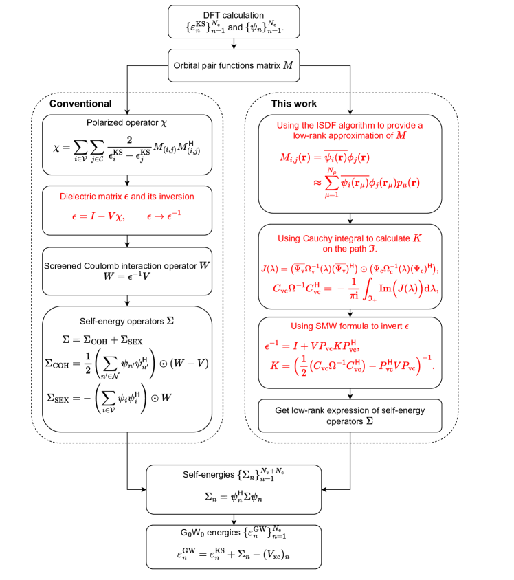
Figure 1: Flowchart difference between conventional and low-rank G₀W₀ calculations. The inversion step is highlighted.

2.2 Errors of self-energies

Our improved method produces approximation errors of self-energies from both the ISDF algorithm and numerical quadrature of Cauchy integral, and are bounded with

$$\mathcal{O}\bigl{(}\delta M+\mathrm{e}^{-N_{\lambda}/C}\bigr{)}.$$ (1)

Here, $\delta M$ refers to the errors introducing by the ISDF algorithm to the orbital pair functions matrix $M$, $N_{\lambda}$ is the number of quadrature nodes in Cauchy integral, and $C$ is the condition number related to the bandgap of the system. More precise expressions of these terms in the error bound will be given in (18) and (3.6), respectively, and the error analysis can be found in Section 3.6. We highlight two key facts here. First, an accurate strategy in the ISDF algorithm is necessary because the error bound in equation (1) requires a good approximation of $M$. Second, the bound given by (1) is pessimistic. Numerical experiments show that a much accurate result can be expected for real systems.

We first investigate the effect of errors in the ISDF algorithm. Our improved strategy applies the ISDF algorithm to the orbital pair functions matrix $M$ of different sets. Different combinations of $M$ are used in different steps in our improved strategy. The product of occupied and unoccupied states is used to construct operators in the fast-inversion strategy, and other combinations are used to construct four-center two-electron integrals and manipulate self-energies in our improved GW strategy. We need to treat them separately since they have different effects on the errors of self-energies. To illustrate the effect of errors in the ISDF algorithm, we vary the ISDF coefficients in different combinations of $M$. We first change the ISDF coefficient with respect to occupied and unoccupied states, denoted by $k_{\mathrm{vc}}$, and fix the other ISDF coefficients, denoted by $k_{\mathrm{vn}}$ and $k_{\mathrm{nn}}$ to $8.0$. Then we fix the ISDF coefficient of the first one to $8.0$ and vary the other ISDF coefficients.

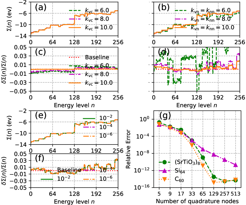
Figure 2: Errors of self-energies for Si₆₄ in improved GW calculation strategy. (a) and (c): The ISDF coefficient $k_{\mathrm{vn}}$ and $k_{\mathrm{nn}}$ are fixed to $8.0$, and $k_{\mathrm{vc}}$ varies from $6.0$ to $10.0$. (b) and (d): The ISDF coefficient $k_{\mathrm{vc}}=8.0$ is fixed, and $k_{\mathrm{vn}}=k_{\mathrm{nn}}$ varies from $6.0$ to $10.0$. The green, purple, and orange lines in (d) represent $k_{\mathrm{vn}}=k_{\mathrm{nn}}=6.0$, $k_{\mathrm{vn}}=k_{\mathrm{nn}}=8.0$, and $k_{\mathrm{vn}}=k_{\mathrm{nn}}=10.0$, respectively. (a) to (d) do not involve Cauchy integral. (e) and (f): The ISDF coefficients $k_{\mathrm{vc}}=k_{\mathrm{vn}}=k_{\mathrm{nn}}=8.0$ are fixed, and the upper bound of the relative error of Cauchy integral result in Algorithm 2 varies from $10^{-2}$ to $10^{-6}$. (g): Errors of Cauchy integral in terms of the number of quadrature nodes.

The results, as shown in Figs. 2 (a) to (d), reveal the following two facts. First, increasing any ISDF coefficients can reduce the relative errors on self-energies as expected. Second, comparing Figs. 2 (c) and (d) when $k=6.0$, we notice that the taking $k_{\mathrm{vn}}=k_{\mathrm{nn}}=6.0$ produces much larger relative error compared to taking $k_{\mathrm{vc}}=6.0$. Hence, self-energies are much more sensitive to $k_{\mathrm{vn}}$ and $k_{\mathrm{nn}}$ than $k_{\mathrm{vc}}$. The reason is that $k_{\mathrm{vc}}$ affects the operators’ calculation, which has only indirect impact to self-energies, whereas $k_{\mathrm{vn}}$ and $k_{\mathrm{nn}}$ affect the self-energies calculation straightway. It is worth mentioning that both time complexity and space complexity of our method is quadratic in terms of the ISDF coefficients (see Table 2). Balancing is needed between accuracy and efficiency. The experiment above shows that it is possible to choose a smaller value of $k_{\mathrm{vc}}$ and larger values of $k_{\mathrm{vn}}$ and $k_{\mathrm{nn}}$ to accelerate the calculation while ensuring the relative accuracy of the self-energies.

Then we show the relationship between the quadrature error in Cauchy integral and the error of self-energies. Algorithm 2 explains how to adopt Cauchy integral in our strategy with adaptive refinement. The algorithm provides a result based on a given threshold that also bounds the quadrature error. We still use Si₆₄ as a case study and set different upper bounds on the relative error in Algorithm 2 to demonstrate the relationship between the errors. We present our computational results in Figs. 2 (e) to (g). Figs. 2 (e) and (f) show that with quadrature error ranging from $10^{-2}$ to $10^{-6}$, the corresponding error curves for the self-energies are closely intertwined. This observation suggests that the error of Cauchy integral has marginal impact on the accuracy of the self-energies. This allows us to choose a loose error estimate for Algorithm 2 without impacting the accuracy of self-energies.

Our quadrature rule is an adaptive one that automatically refines the partition. As the quadrature error decreases geometrically with respect to the number of quadrature nodes, the cost of numerical quadrature is moderately small. Numerical tests in Fig. 2 (g) agree with our analysis. By quadaturing with $513$ nodes, the quadrature error already drops to a satisfactory level, indicating that it is easy to achieve a negligible relative error of Cauchy integral for both molecular and solid systems. Hence it is not really important to balance between efficiency and accuracy in calculating Cauchy integral.

2.3 Low-rank properties for functions and operators

The ISDF algorithm and Sherman–Morrison–Woodbury formula assume that both the orbital pair functions matrix $M$ and the polarizability matrix $\chi$ have certain low-rank properties. This assumption is usually plausible in practice. We take Si₆₄ and (SrTiO₃)₈ as examples to demonstrate the decay of singular values for both $M$ and $\chi$.

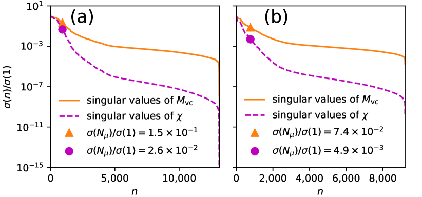
Figure 3: Singular values of conventional $M_{\mathrm{vc}}$ and $\chi$ in (a) Si₆₄ and (b) (SrTiO₃)₈. Here, $k_{\mathrm{vc}}=8.0$, $N_{\mu}=k_{\mathrm{vc}}\sqrt{N_{\mathrm{v}}N_{\mathrm{c}}}$, $N_{\mathrm{v}}$ and $N_{\mathrm{c}}$ are given in Table 1 of Supplementary information.

Numerical experiments in Fig. 3 show that when $k_{\mathrm{vc}}=8.0$, the ISDF algorithm introduces a relative error of $\Theta(10^{-1})$ to $M_{\mathrm{vc}}$ in both systems and a relative error of $\Theta(10^{-2})$ to $\chi$ in Si₆₄. The decay pattern of the singular values is system-dependent, as illustrated in Fig. 3. The singular values of both $\chi$ and $M_{\mathrm{vc}}$ in Si₆₄ decay rapidly but smoothly, while $\chi$ in (SrTiO₃)₈ has a much faster decay in its leading singular values. This rapid-decay phenomenon is strongly associated with the pattern of orbital pair functions matrix $M_{\mathrm{vc}}$, as the leading singular values of the orbital pair functions matrix $M_{\mathrm{vc}}$ of (SrTiO₃)₈ decrease much faster than that of Si₆₄.

We remark that though errors introduced by the ISDF algorithm to $M$ and $\chi$ can be pretty large at the first glance, results in Fig. 2 suggest that the self-energies can still be computed with satisfactory accuracy.

2.4 Computational complexity

Silicon bulk systems are known for their symmetry and highly extendible properties. In this study, we demonstrate the effectiveness of our method using Si₈, Si₁₆, Si₃₂, and Si₆₄, in terms of time complexity. We compare our strategy with the conventional G₀W₀ calculation strategy, the strategy by Ma et al. [22], all implemented in MATLAB. The test result of the Fortran-based package BerkeleyGW, which uses the conventional G₀W₀ strategy, is also listed for reference. In this test, we only use a single processor.

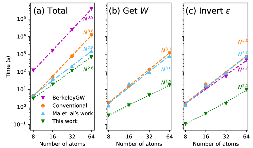
Figure 4: Total time for the conventional strategy, strategy from [22] and our improved strategy on Si with different bulk sizes. The ISDF coefficients are set to be $8.0$, and the threshold for Cauchy integral is set to be $10^{-7}$. (a) Execution time from calculating all operators to calculating self-energies in G₀W₀ calculation. The time for ISDF algorithm is included. (b) Execution time until obtaining the screened Coulomb interaction matrix $W$, excluding the time for ISDF. BerkeleyGW is not listed here as its implementation is a bit different so that it is not easy to make a fair comparison. (c) Total execution time for inverting $\epsilon$.

Fig. 4 shows that our strategy significantly reduces the time required for G₀W₀ calculation compared to other strategies. Our main improvement in the inversion of the dielectric matrix leads to about $10\times$ speedup compared to other alternatives already for these small systems. The benefit of our strategy becomes more and more significant as the problem size grows, because our strategy also has a lower asymptotic scaling than other strategies.

We list the complexity of each algorithm in Table 2 (BerkeleyGW is as same as the conventional strategy). Let us take the strategy from [22] as an example. The time complexity of this strategy is $\mathcal{O}({N_{\mathrm{r}}^{3}+k_{\mathrm{vc}}^{2}N_{\mathrm{e}}^{4}})$, where $N_{\mathrm{r}}\sim 1000N_{\mathrm{e}}$. The cubic term dominates for small systems with tens of electrons because $N_{\mathrm{r}}$ is very large compared to $N_{\mathrm{e}}$. The corresponding curve in Fig. 4 (a) stays low, and is expected to grow rapidly for larger systems.

We also notice that BerkeleyGW, a Fortran-based high-performance computing package, performs much more slowly than our MATLAB-based version. The main reason is that several computationally intensive steps in BerkeleyGW do not utilize level-3 BLAS, resulting in a significant loss of computational efficiency. As a well-developed package, BerkeleyGW supports multiple $k$-points calculation, and manages to use a unified approach to handle the $\Gamma$-point (also known as the single $k$-point) and multiple $k$-points. Such a unified approach is based on several do loops, making the most computational intensity part of the self-energies calculation elementwise. However, in the MATLAB version we do not support $k$-points yet. This allows us to easily perform the computation using well-developed level-3 BLAS.

3 Methods

3.1 GW approximation

GW approximation expresses one-particle excitation energies with quasiparticle equation as

$$\Bigl{(}-\frac{1}{2}\nabla^{2}+V_{\mathrm{ion}}(\mathbf{r})+V_{\mathrm{H}}(\mathbf{r})\Bigr{)}\psi_{i}^{\mathrm{QP}}(\mathbf{r})+\int_{\mathbb{R}^{3}}\mathop{}\mathopen{}\mathrm{d}\mathbf{r}^{\prime}\Sigma\bigl{(}\mathbf{r},\mathbf{r}^{\prime};\varepsilon_{i}^{\mathrm{GW}}\bigr{)}\psi_{i}^{\mathrm{QP}}(\mathbf{r}^{\prime})=\varepsilon_{i}^{\mathrm{GW}}\psi_{i}^{\mathrm{QP}}(\mathbf{r}),$$ (2)

where $\Sigma$ is the self-energy operator in frequency space [6, 24], $\psi^{\mathrm{QP}}_{i}$’s are the quasiparticle wavefunctions, and $\varepsilon_{i}^{\mathrm{GW}}$’s refer to quasiparticle energies. We assume spin deformation and zero-temperature in this work so that the spin variables are ignored. Also, we only consider the case of $\Gamma$-point, and hence indices of $k$-points are excluded.

The self-energy operator can be expressed by the Green’s functions $G$ and the screened Coulomb potential $W$ as

$$\Sigma(\mathbf{r},\mathbf{r}^{\prime};\omega)={} \frac{\mathrm{i}}{2\pi}\int_{\mathbb{R}}\mathrm{e}^{-\mathrm{i}\omega^{\prime}\eta}G(\mathbf{r},\mathbf{r}^{\prime};\omega-\omega^{\prime})W(\mathbf{r},\mathbf{r}^{\prime};\omega^{\prime})\mathop{}\mathopen{}\mathrm{d}\omega^{\prime}.$$

Here, $\eta$ is a small frequency shift to guarantee convergence. We use Lehmann representation of the one-particle Green’s functions $G$ with a set of quasiparticle wavefunctions

$$G(\mathbf{r},\mathbf{r}^{\prime};\omega)=\sum_{n\in\mathcal{N}}\frac{\psi_{i}^{\mathrm{QP}}(\mathbf{r})\overline{\psi_{i}^{\mathrm{QP}}(\mathbf{r}^{\prime})}}{\omega-\varepsilon_{i}^{\mathrm{QP}}+\mathrm{i}\operatorname{sign}(\varepsilon_{n}-\mu)\eta},$$ (3)

and use a set of Hedin’s equations to generate the screened Coulomb potential operator $W$ as

$$\begin{split}W(\mathbf{r},\mathbf{r}^{\prime};\omega)={}&\int_{\mathbb{R}^{3}}\mathop{}\mathopen{}\mathrm{d}\mathbf{r}^{\prime\prime}\epsilon^{-1}(\mathbf{r},\mathbf{r}^{\prime\prime};\omega)V(\mathbf{r}^{\prime\prime},\mathbf{r}^{\prime}),\\ \epsilon(\mathbf{r},\mathbf{r}^{\prime};\omega)={}&\delta(\mathbf{r}-\mathbf{r}^{\prime})-\int_{\mathbb{R}^{3}}\mathop{}\mathopen{}\mathrm{d}\mathbf{r}^{\prime\prime}V(\mathbf{r},\mathbf{r}^{\prime\prime})\chi(\mathbf{r}^{\prime\prime},\mathbf{r}^{\prime};\omega),\\ \chi(\mathbf{r},\mathbf{r}^{\prime};\omega)={}&\sum_{i\in\mathcal{V}}\sum_{j\in\mathcal{C}}\psi^{\mathrm{QP}}_{i}(\mathbf{r})\overline{\psi^{\mathrm{QP}}_{j}(\mathbf{r})}\overline{\psi^{\mathrm{QP}}_{i}(\mathbf{r}^{\prime})}\psi^{\mathrm{QP}}_{j}(\mathbf{r}^{\prime})\cdot\frac{1}{\omega+\varepsilon_{i}-\varepsilon_{j}+\mathrm{i}\eta}\\ &-\sum_{i\in\mathcal{V}}\sum_{j\in\mathcal{C}}\overline{\psi^{\mathrm{QP}}_{i}(\mathbf{r})}{\psi^{\mathrm{QP}}_{j}(\mathbf{r})}{\psi^{\mathrm{QP}}_{i}(\mathbf{r}^{\prime})}\overline{\psi^{\mathrm{QP}}_{j}(\mathbf{r}^{\prime})}\cdot\frac{1}{\omega-\varepsilon_{i}+\varepsilon_{j}-\mathrm{i}\eta}.\end{split}$$ (4)

The operators on the left-hand side are, respectively, the screened Coulomb interaction operator, the dielectric operator, and the polarizability operator, and $V(\mathbf{r},\mathbf{r}^{\prime})$ refers to the Coulomb interaction.

The simplest GW calculation is the one-shot GW, also known as G₀W₀. The standard procedure of G₀W₀ is first getting the ground-states information from DFT, and then replacing quasiparticle energies and wavefunctions in equations above with the ground-states ones. G₀W₀ can be implemented by several commonly used approximations, including the static COulomb Hole plus Screened EXchange (COHSEX) approximation [6, 24], the full-frequency approximation [25, 26], and the generalized plasmon–pole approximation (GPP) [27]. To show the feasibility of our low-rank strategy of inverting the dielectric matrix $\epsilon$ in the framework of GW calculation, we use the static COHSEX approximation. In the static COHSEX approximation, we set the frequency to be $0$ in the screened Coulomb interaction operator $W$ and let the Green’s function $G$ to be a non-interacting one.

The self-energy operator $\Sigma$ under the static COHSEX approximation can be separated into

$$\Sigma_{\mathrm{COHSEX}}(\mathbf{r},\mathbf{r}^{\prime})=\Sigma_{\mathrm{COH}}(\mathbf{r},\mathbf{r}^{\prime})+\Sigma_{\mathrm{SEX}}(\mathbf{r},\mathbf{r}^{\prime}),$$

where the screened exchange part (SEX) and Coulomb hole part (COH), respectively, are expressed as

$$\Sigma_{\mathrm{COH}}(\mathbf{r},\mathbf{r}^{\prime}) =\frac{1}{2}\delta(\mathbf{r}-\mathbf{r}^{\prime})\bigl{(}W(\mathbf{r},\mathbf{r}^{\prime};\omega=0)-V(\mathbf{r},\mathbf{r}^{\prime})\bigr{)},$$ (5)

$$\Sigma_{\mathrm{SEX}}(\mathbf{r},\mathbf{r}^{\prime}) =-\sum_{i\in\mathcal{V}}\psi_{i}(\mathbf{r})\overline{\psi_{i}(\mathbf{r}^{\prime})}W(\mathbf{r},\mathbf{r}^{\prime};\omega=0).$$

After discretization in real space, dropping the frequency variable, and substituting (4) into (5), while noting that the two parts of $\chi$ are complex conjugates of each other, we obtain

$$\chi(\mathbf{r},\mathbf{r}^{\prime})={} 2\mathop{\mathrm{Re}}\sum_{i\in\mathcal{V}}\sum_{j\in\mathcal{C}}\psi_{i}(\mathbf{r})\overline{\psi_{i}(\mathbf{r}^{\prime})}\psi_{j}(\mathbf{r}^{\prime})\overline{\psi_{j}(\mathbf{r})}\cdot\frac{1}{\varepsilon_{i}^{\mathrm{KS}}-\varepsilon_{j}^{\mathrm{KS}}},$$ (6)

$$\epsilon(\mathbf{r},\mathbf{r}^{\prime})={} \delta(\mathbf{r}-\mathbf{r}^{\prime})-\sum_{\mathbf{r}^{\prime\prime}}V(\mathbf{r},\mathbf{r}^{\prime\prime})\chi(\mathbf{r}^{\prime\prime},\mathbf{r}^{\prime}),$$

$$W(\mathbf{r},\mathbf{r}^{\prime})={} \sum_{\mathbf{r}^{\prime\prime}}\epsilon^{-1}(\mathbf{r},\mathbf{r}^{\prime\prime})V(\mathbf{r}^{\prime\prime},\mathbf{r}^{\prime}),$$

$$\Sigma_{\mathrm{SEX}}(n)={} \sum_{\mathbf{r},\mathbf{r}^{\prime}}\overline{\psi_{n}(\mathbf{r})}\psi_{n}(\mathbf{r}^{\prime})\Sigma_{\mathrm{SEX}}(\mathbf{r},\mathbf{r}^{\prime})$$

$$={} -\sum_{i\in\mathcal{V}}\sum_{\mathbf{r},\mathbf{r}^{\prime}}\sum_{\mathbf{r}^{\prime\prime}}\psi_{i}(\mathbf{r})\overline{\psi_{n}(\mathbf{r})}\overline{\psi_{i}(\mathbf{r}^{\prime})}\psi_{n}(\mathbf{r}^{\prime})\epsilon^{-1}(\mathbf{r},\mathbf{r}^{\prime\prime})V(\mathbf{r}^{\prime\prime},\mathbf{r}^{\prime}),$$

$$\Sigma_{\mathrm{COH}}(n)= \sum_{\mathbf{r},\mathbf{r}^{\prime}}\overline{\psi_{n}(\mathbf{r})}\psi_{n}(\mathbf{r}^{\prime})\Sigma_{\mathrm{COH}}(\mathbf{r},\mathbf{r}^{\prime})$$

$$={} \frac{1}{2}\sum_{n^{\prime}\in{\mathcal{N}}}\sum_{\mathbf{r},\mathbf{r}^{\prime}}\sum_{\mathbf{r}^{\prime\prime}}\psi_{n^{\prime}}(\mathbf{r})\overline{\psi_{n}(\mathbf{r})}\overline{\psi_{n^{\prime}}(\mathbf{r}^{\prime})}\psi_{n}(\mathbf{r}^{\prime})\bigl{(}\epsilon^{-1}(\mathbf{r},\mathbf{r}^{\prime\prime})-\delta(\mathbf{r},\mathbf{r}^{\prime\prime})\bigr{)}V(\mathbf{r}^{\prime\prime},\mathbf{r}^{\prime}).$$

Here, we use $\Sigma(n)$ to denote the self-energy of the band level $n$, and use $\Sigma(\mathbf{r},\mathbf{r}^{\prime})$ or $\Sigma$ to denote the self-energy operator. We separate the bare Coulomb part from the screened exchange part of the self-energy operator $\Sigma_{\mathrm{SEX}}$ as

$$\Sigma_{\mathrm{SEX}}={} \Sigma_{\mathrm{SEX\_X}}+\Sigma_{\mathrm{X}},$$ (7)

$$\Sigma_{\mathrm{SEX\_X}}(n)={} -\sum_{i\in{\mathcal{V}}}\sum_{\mathbf{r},\mathbf{r}^{\prime}}\psi_{i}(\mathbf{r})\overline{\psi_{n}(\mathbf{r})}\overline{\psi_{i}(\mathbf{r}^{\prime})}\psi_{n}(\mathbf{r}^{\prime})\bigl{(}\epsilon^{-1}(\mathbf{r},\mathbf{r}^{\prime})-\delta(\mathbf{r},\mathbf{r}^{\prime})\bigr{)}V(\mathbf{r},\mathbf{r}^{\prime}),$$

$$\Sigma_{\mathrm{X}}(n)={} -\sum_{i\in{\mathcal{V}}}\sum_{\mathbf{r},\mathbf{r}^{\prime}}\psi_{i}(\mathbf{r})\overline{\psi_{n}(\mathbf{r})}\overline{\psi_{i}(\mathbf{r}^{\prime})}\psi_{n}(\mathbf{r}^{\prime})V(\mathbf{r},\mathbf{r}^{\prime}).$$

For simplicity, we assume time-reversal symmetry in the system. For the G₀W₀ calculation with only $\Gamma$-point, time-reversal symmetry becomes

$$\overline{\psi_{n}(\mathbf{r})}=\psi_{n}(\mathbf{r}),\quad\forall n,$$ (8)

which means the wavefunctions are real in real space. However, we continue to treat the wavefunctions $\psi(\mathbf{r})$ as a complex value to align with the general G₀W₀ framework. Under the time-reversal symmetry assumption (8), we obtain the matrix forms of all operators in (6) as

$$\chi=2{M_{\mathrm{vc}}}\Omega^{-1}({M_{\mathrm{vc}}})^{\mathsf{H}},\qquad\epsilon=I-V\chi_{0},\qquad W=\epsilon^{-1}V,\\$$ (9)

and components of the self-energies in (7) become

$$\Sigma_{\mathrm{SEX\_X}}(n) =-\sum_{i\in\mathcal{V}}\bigl{(}\psi_{n}\odot\overline{\psi_{i}}\bigr{)}^{\mathsf{H}}(W-V)\bigl{(}\psi_{n}\odot\overline{\psi_{i}}\bigr{)},$$

$$\Sigma_{\mathrm{X}}(n) =-\sum_{i\in\mathcal{V}}\bigl{(}\psi_{n}\odot\overline{\psi_{i}}\bigr{)}^{\mathsf{H}}V\bigl{(}\psi_{n}\odot\overline{\psi_{i}}\bigr{)},$$

$$\Sigma_{\mathrm{COH}}(n) =\frac{1}{2}\sum_{n^{\prime}\in\mathcal{N}}\bigl{(}\psi_{n}\odot\overline{\psi_{n^{\prime}}}\bigr{)}^{\mathsf{H}}(W-V)\bigl{(}\psi_{n}\odot\overline{\psi_{n^{\prime}}}\bigr{)}.$$

In (9), $\Omega$ refers to a diagonal matrix with elements

$$\Omega_{(i,j;k,l)}=\delta_{i,k}\delta_{j,l}(\varepsilon_{i}^{\mathrm{KS}}-\varepsilon_{j}^{\mathrm{KS}}),\qquad i,k\in\mathcal{V},\quad j,l\in\mathcal{C},$$ (10)

and the matrix $M_{\mathrm{vc}}$ refers to orbital pair functions of all occupied and unoccupied states, i.e.,

$$\bigl{(}M_{\mathrm{vc}}\bigr{)}_{(n;i,j)}=\overline{\psi_{i}(\mathbf{r}_{n})}{\psi_{j}(\mathbf{r}_{n})},\qquad i\in\mathcal{V},\quad j\in\mathcal{C}.$$

Here, the pair $(i,j)$ together forms the column index of the matrix.

As we have mentioned before, both time complexity and space complexity of the G₀W₀ calculation are pretty high. Evaluating $\chi$ as a matrix costs $\mathcal{O}({N_{\mathrm{e}}^{4}})$; inverting $\epsilon$ costs $\mathcal{O}({N_{\mathrm{e}}^{3}})$ with a huge prefactor; and calculating $\Sigma$ conventionally costs $\mathcal{O}({N_{\mathrm{e}}^{5}})$. Space complexity is also a great burden in the GW calculation, as manipulating $\chi$ requires to store orbital pair functions of all occupied and unoccupied orbitals, which costs $\mathcal{O}({N_{\mathrm{e}}^{3}})$. The high complexity limits the practical application of GW calculation.

3.2 Interpolative separable density fitting

We use the Interpolative Separable Density Fitting (ISDF) algorithm [19] to reduce the time complexity of evaluating $\chi$. The ISDF algorithm represents the orbital pair functions $M_{i,j}(\mathbf{r})$ as

$$M_{i,j}(\mathbf{r})=\overline{\psi_{i}(\mathbf{r})}{\phi_{j}(\mathbf{r})}\thickapprox\sum\limits_{\mu=1}^{N_{\mu}}\overline{\psi_{i}({\mathbf{r}_{\mu}})}{\phi_{j}({\mathbf{r}_{\mu}})}p_{\mu}(\mathbf{r}),$$ (11)

where $N_{\mu}$ in (11) refers to the number of auxiliary functions. There are several choices on the interpolation points $\{\mathbf{r}_{\mu}\}_{\mu=1}^{N_{\mu}}$ and auxiliary functions $\{p_{\mu}(\mathbf{r})\}_{\mu=1}^{N_{\mu}}$ in the ISDF algorithm, such as QRCP and $k$-means [28, 18]. We represent (11) in matrix form as

$$M=PC,$$ (12)

where

$$M_{(n;i,j)}=\overline{\psi_{i}(\mathbf{r}_{n})}{\phi_{j}(\mathbf{r}_{n})},\qquad P_{(n;\mu)}=p_{\mu}(\mathbf{r}_{n}),\qquad C_{(\mu;i,j)}=\overline{\psi_{i}(\mathbf{r}_{\mu})}{\phi_{j}(\mathbf{r}_{\mu})}.$$

Numerical experiments suggest that as the number of wavefunctions increases, $N_{\mu}$ needs to grow linearly with respect to the number of wavefunctions to keep the relative error constant [18]. Base on this observation, we set

$$N_{\mu}=k_{\mu}\sqrt{N_{1}N_{2}},$$

where $N_{1}$ and $N_{2}$ are the numbers of wavefunctions in two sets, respectively, and $k_{\mu}$ is a small constant of $\Theta(10^{1})$.

Ma et al. implemented the ISDF algorithm in GW calculation [22]. Their approach is summarized in Algorithm 1. By using the ISDF algorithm, Algorithm 1 greatly reduces the dominant quartic term in the time complexity. The memory requirement is also largely reduced. However, this algorithm requires an explicit expression of the ISDF coefficient matrix $C_{\mathrm{vc}}$, which consumes $\mathcal{O}({N_{\mathrm{e}}^{3}})$ storage. Moreover, the cubic terms in time complexity still have ultra-high prefactors since their approach inverts $\epsilon$ explicitly.

Algorithm 1 Implement the ISDF algorithm on G₀W₀ calculation, from Ma et al. [22].

0.8

0:  KS–DFT wavefunctions ${\{\psi_{i}\}}_{i=1}^{N_{\mathrm{v}}+N_{\mathrm{c}}}$, KS–DFT band energies $\{\varepsilon_{i}^{\mathrm{KS}}\}_{i=1}^{N_{\mathrm{v}}+N_{\mathrm{c}}}$, exchange and correlation energies $\{{(V_{\mathrm{xc}})}_{i}\}_{i=1}^{N_{\mathrm{v}}+N_{\mathrm{c}}}$, indices of interpolation points and auxiliary function matrices $\{P\}$ from the ISDF algorithm.

0:  GW energy ${\{\varepsilon^{\mathrm{GW}}_{i}\}}_{i=1}^{N_{\mathrm{v}}+N_{\mathrm{c}}}$.

1:  Calculate $\mathcal{O}({k_{\mu}N_{\mathrm{e}}N_{\mathrm{r}}^{2}+k_{\mu}^{2}N_{\mathrm{e}}^{4}})$

$$\chi=2M_{\mathrm{vc}}\Omega^{-1}M_{\mathrm{vc}}^{\mathsf{H}},\qquad\epsilon=I-V\chi.$$

2:  Calculate $\epsilon^{-1}$ by LU decomposition. $\mathcal{O}({N_{\mathrm{r}}^{3}})$

3:  Calculate screened Coulomb interaction matrix $\mathcal{O}({N_{\mathrm{r}}^{2}})$

$$W_{\mathrm{V}}=W-V=(\epsilon^{-1}-I)V.$$

4:  Calculate$\mathcal{O}({k_{\mu}N_{\mathrm{e}}N_{\mathrm{r}}^{2}})$

$$W_{\mathrm{vn}}=P_{\mathrm{vn}}^{\mathsf{H}}W_{\mathrm{V}}P_{\mathrm{vn}},\qquad W_{\mathrm{nn}}=P_{\mathrm{nn}}^{\mathsf{H}}W_{\mathrm{V}}P_{\mathrm{nn}},\qquad V_{\mathrm{vn}}=P_{\mathrm{vn}}^{\mathsf{H}}VP_{\mathrm{vn}}.$$

5:  Calculate the part of self-energies induced from the screened exchange interaction $\mathcal{O}({k_{\mu}^{2}N_{\mathrm{e}}^{3}})$

$$\Sigma_{\mathrm{SEX\_X}}={} \sum_{i\in\mathcal{V}}(\overline{\psi_{i}^{\mathrm{vn}}})^{\mathsf{H}}\Bigl{(}W_{\mathrm{vn}}\odot\bigl{(}\Psi^{\mathrm{vn}}{(\Psi^{\mathrm{vn}})}^{\mathsf{H}}\bigr{)}\Bigr{)}(\overline{\psi_{i}^{\mathrm{vn}}}),$$

$$\Sigma_{\mathrm{X}}={} \sum_{i\in\mathcal{V}}(\overline{\psi_{i}^{\mathrm{vn}}})^{\mathsf{H}}\Bigl{(}V_{\mathrm{vn}}\odot\bigl{(}\Psi^{\mathrm{vn}}{(\Psi^{\mathrm{vn}})}^{\mathsf{H}}\bigr{)}\Bigr{)}(\overline{\psi_{i}^{\mathrm{vn}}}).$$

6:  Calculate the part of self-energies induced from the Coulomb hole interaction $\mathcal{O}({k_{\mu}^{2}N_{\mathrm{e}}^{3}})$

$$\Sigma_{\mathrm{COH}}={} \sum_{i\in\mathcal{N}}(\overline{\psi_{i}^{\mathrm{nn}}})^{\mathsf{H}}\Bigl{(}W_{\mathrm{nn}}\odot\bigl{(}\Psi^{\mathrm{nn}}{(\Psi^{\mathrm{nn}})}^{\mathsf{H}}\bigr{)}\Bigr{)}(\overline{\psi_{i}^{\mathrm{nn}}}).$$

7:  Calculate self-energies

$$\Sigma=\mathop{\mathrm{Re}}\bigl{(}\operatorname{diag}({\Sigma_{\mathrm{SEX\_X}}+\Sigma_{\mathrm{X}}+\Sigma_{\mathrm{COH}}})\bigr{)}.$$

8:  Calculate quasiparticle energies under G₀W₀ approximation

$$\varepsilon^{\mathrm{GW}}_{i}=\varepsilon_{i}^{\mathrm{KS}}+\Sigma_{i}-{(V_{\mathrm{xc}})}_{i}.$$

3.3 Sherman–Morrison–Woodbury (SMW) formula combined with ISDF

Suppose that both $A$ and $A+UV^{\mathsf{H}}$ are $n\times n$ nonsingular matrices, where $U$, $V\in\mathbb{C}^{n\times k}$. Then the Sherman–Morrison–Woodbury (SMW) formula [29] reads

$$(A+UV^{\mathsf{H}})^{-1}=A^{-1}-A^{-1}U(I+V^{\mathsf{H}}A^{-1}U)^{-1}V^{\mathsf{H}}A^{-1}.$$ (13)

Liu et al. in [10] suggest that by SMW formula, the inverse of dielectric matrix, $\epsilon^{-1}(\omega)$, can be decomposed into a sum of rank-$1$ matrices as follows

$$\epsilon^{-1}(\omega)=I+\sum_{l=1}^{N_{\mathrm{v}}N_{\mathrm{c}}}\frac{1}{2\sqrt{\lambda_{l}}}V(M_{\mathrm{vc}}s_{l})\Bigl{(}\frac{1}{\omega-\sqrt{\lambda_{l}}+\mathrm{i}\eta}-\frac{1}{\omega+\sqrt{\lambda_{l}}+\mathrm{i}\eta}\Bigr{)}(M_{\mathrm{vc}}s_{l})^{\mathsf{H}},$$ (14)

where $s_{l}=\Omega^{1/2}u_{l}$, $\Omega$ is the same as in (10), and $\{(\lambda_{l},u_{l})\}_{l=1}^{N_{\mathrm{v}}N_{\mathrm{c}}}$ are the eigenpairs of $\Omega^{2}+\Omega^{1/2}M^{\mathsf{H}}VM\Omega^{1/2}$.

Once the eigenpairs of the system described above are known, we can write the screened exchange part and the Coulomb hole part of the self-energy matrices as

$$\Sigma_{\mathrm{SEX\_X}}=-\sum_{i\in\mathcal{V}}(\psi_{i}\psi_{i}^{\mathsf{H}})\odot\Biggl{(}\sum_{l=1}^{N_{\mathrm{v}}N_{\mathrm{c}}}\frac{1}{2\sqrt{\lambda_{l}}}\frac{(VM_{\mathrm{vc}}s_{l})(VM_{\mathrm{vc}}s_{l})^{\mathsf{H}}}{\omega-\varepsilon_{i}^{\mathrm{KS}}-\sqrt{\lambda_{l}}}\Biggr{)},$$

$$\Sigma_{\mathrm{COH}}=\frac{1}{2}\sum_{i\in\mathcal{N}}(\psi_{i}\psi_{i}^{\mathsf{H}})\odot\Biggl{(}\sum_{l=1}^{N_{\mathrm{v}}N_{\mathrm{c}}}\frac{1}{2\sqrt{\lambda_{l}}}\frac{(VM_{\mathrm{vc}}s_{l})(VM_{\mathrm{vc}}s_{l})^{\mathsf{H}}}{\omega-\varepsilon_{i}^{\mathrm{KS}}-\sqrt{\lambda_{l}}}\Biggr{)}.$$

However, (14) requires all eigenvectors of an $N_{\mathrm{v}}N_{\mathrm{c}}\times N_{\mathrm{v}}N_{\mathrm{c}}$ dense Hermite matrix, resulting in a time complexity of $\mathcal{O}({N_{\mathrm{e}}^{6}})$. This is too expensive for practical computation.

In order to develop a cubic scaling algorithm for computing $\epsilon^{-1}$, we propose an alternative approach to apply the SMW formula. To simplify the notation, we does not distinguish the operators and their matrix representations obtained through discretization. Superscripts on the energies $\varepsilon$’s are also omitted.

Note that the ISDF algorithm expresses the orbital pair functions matrix $M{{}_{\mathrm{vc}}}$ as (12). We substitute (12) into the expression of the polarizability matrix $\chi$ and the dielectric matrix $\epsilon$ in (9), and obtain the matrix representations of $\chi$ and $\epsilon$ as

$$\chi =2P{{}_{\mathrm{vc}}}C{{}_{\mathrm{vc}}}\Omega^{-1}(P{{}_{\mathrm{vc}}}C{{}_{\mathrm{vc}}})^{\mathsf{H}},$$

$$\epsilon =I-2V(P{{}_{\mathrm{vc}}}C{{}_{\mathrm{vc}}})\Omega^{-1}(P{{}_{\mathrm{vc}}}C{{}_{\mathrm{vc}}})^{\mathsf{H}}.$$

Applying the SMW formula to invert the dielectric matrix $\epsilon$, we have

$$\epsilon^{-1}=I+VP_{\mathrm{vc}}\Bigl{(}\frac{1}{2}({C{{}_{\mathrm{vc}}}\Omega^{-1}C_{\mathrm{vc}}^{\mathsf{H}}})^{-1}-P_{\mathrm{vc}}^{\mathsf{H}}VP_{\mathrm{vc}}\Bigr{)}^{-1}P_{\mathrm{vc}}^{\mathsf{H}}.$$ (15)

Clearly (15) is much cheaper than the direct inversion process, because only an $N{{}_{\mathrm{vc}}}\times N{{}_{\mathrm{vc}}}$ matrix needs to be explicitly inverted. Additionally, explicit formulation of $\chi$ and $\epsilon$ is avoided. Therefore, (15) significantly reduces the time complexity of the inversion process.

We remark that directly applying SMW as (15) is still not fully satisfactory. The ISDF algorithm provides low-rank properties to the screened Coulomb interaction operator $W$ and the self-energy operator $\Sigma$. The low-rank properties are not exploited in the conventional G₀W₀ calculation strategy. Even if (15) is adopted, further computation in the G₀W₀ calculation still involves $N_{\mathrm{r}}\times N_{\mathrm{r}}$ matrices. Also, we need an explicit expression of the ISDF coefficient matrix $C_{\mathrm{vc}}$ in (15), which is $N_{\mu}\times N_{\mathrm{v}}N_{\mathrm{c}}$. As inverting $\epsilon$ requires calculating ${C{{}_{\mathrm{vc}}}\Omega^{-1}C_{\mathrm{vc}}^{\mathsf{H}}}$ first, our calculation still costs the time complexity of $\mathcal{O}({N_{\mathrm{e}}^{4}})$ and space complexity of $\mathcal{O}({N_{\mathrm{e}}^{3}})$. Therefore, we shall tackle these issues in subsequent subsections.

3.4 Cauchy integral representation

In [20], Lu and Thicke suggest that the time complexity of computing $\chi$ can be reduced from $\mathcal{O}({N_{\mathrm{e}}^{4}})$ to $\mathcal{O}({N_{\mathrm{e}}^{3}})$ by using Cauchy integral. Inspired by Lu and Thicke’s work, we propose an algorithm to calculate ${C{{}_{\mathrm{vc}}}\Omega^{-1}C_{\mathrm{vc}}^{\mathsf{H}}}$ with a cubic time complexity, as listed in Algorithm 2. The derivation of Algorithm 2 is explained in detail in Supplementary information.

Algorithm 2 Calculate ${C{{}_{\mathrm{vc}}}\Omega^{-1}C_{\mathrm{vc}}^{\mathsf{H}}}$.

1.0

0:  A matrix $\Psi$ that consists of wavefunctions, indices of interpolative points from the ISDF algorithm, energies $\{\varepsilon_{i}\}_{i=1}^{n}$, a threshold $\delta_{\mathrm{rel}}$.

0:  Coefficient matrix ${C{{}_{\mathrm{vc}}}\Omega^{-1}C_{\mathrm{vc}}^{\mathsf{H}}}$.

1:  Calculate

$$r={}\frac{\sqrt{Q/q}-1}{\sqrt{Q/q}+1},$$

where $q=\varepsilon_{N_{\mathrm{v}}+1}-\varepsilon_{N_{\mathrm{v}}}$ and $Q=\varepsilon_{N_{\mathrm{v}}+N_{\mathrm{c}}}-\varepsilon_{N_{\mathrm{v}}}$.

2:  Calculate

$$R=\int_{0}^{1}\frac{\mathop{}\mathopen{}\mathrm{d}t}{\sqrt{(1-t^{2})(1-r^{2}t^{2})}},\qquad L=\frac{1}{2}\int_{0}^{1/r}\frac{\mathop{}\mathopen{}\mathrm{d}t}{\sqrt{(1+t^{2})(1+r^{2}t^{2})}}.$$

3:  Use an adaptive quadrature rule to calculate

$${C{{}_{\mathrm{vc}}}\Omega^{-1}C_{\mathrm{vc}}^{\mathsf{H}}}=-\frac{\sqrt{Qq}}{\pi\mathrm{i}}\int_{-R+\mathrm{i}L}^{R+\mathrm{i}L}\mathrm{Im}\bigl{(}J(z(t))\bigr{)}\frac{r^{-1}\operatorname{cn}(t)\operatorname{dn}(t)}{(r^{-1}-\operatorname{sn}(t))^{2}}\mathop{}\mathopen{}\mathrm{d}t$$

until the relative error is below the threshold $\delta_{\mathrm{rel}}$, where $J\bigl{(}z\bigr{)}$ is given in (23) of Supplementary information, and

$$z(t)=\sqrt{qQ}\biggl{(}\frac{r^{-1}+\operatorname{sn}(t,r)}{r^{-1}-\operatorname{sn}(t,r)}\biggr{)}+\epsilon_{N_{\mathrm{v}}}.$$

3.5 Cubic scaling algorithm for G₀W₀ calculation

We propose a more efficient and concise version of the G₀W₀ calculation strategy using our fast inversion strategy. Let

$$K={\Bigl{(}\frac{1}{2}{({C{{}_{\mathrm{vc}}}\Omega^{-1}C_{\mathrm{vc}}^{\mathsf{H}}})}^{-1}-P_{\mathrm{vc}}^{\mathsf{H}}VP_{\mathrm{vc}}\Bigr{)}}^{-1}.$$

Then (15) becomes

$$\epsilon^{-1}={}I+VP_{\mathrm{vc}}KP_{\mathrm{vc}}^{\mathsf{H}}.$$

Applying $\epsilon^{-1}$ in (15) to matrices $W{{}_{\mathrm{vc}}}$, $W_{\mathrm{vn}}$, and $W_{\mathrm{nn}}$ in steps 3 and 4 of Algorithm 1 yields

$$V_{\mathrm{vn}}=P_{\mathrm{vn}}^{\mathsf{H}}VP_{\mathrm{vn}},\quad W_{\mathrm{vn}}=\bigl{(}P_{\mathrm{vn}}^{\mathsf{H}}VP_{\mathrm{vc}}\bigr{)}K\bigl{(}P_{\mathrm{vc}}^{\mathsf{H}}VP_{\mathrm{vn}}\bigr{)},\quad W_{\mathrm{nn}}=\bigl{(}P_{\mathrm{nn}}^{\mathsf{H}}VP_{\mathrm{vc}}\bigr{)}K\bigl{(}P_{\mathrm{vc}}^{\mathsf{H}}VP_{\mathrm{nn}}\bigr{)}.$$

Energy matrices under G₀W₀ approximation in steps 5 and 6 of Algorithm 1 can be viewed as

$$\Sigma_{\mathrm{SEX\_X}} =-\sum_{i\in\mathcal{V}}(\overline{\psi_{i}^{\mathrm{vn}}}\odot\Psi^{\mathrm{vn}})^{\mathsf{H}}W_{\mathrm{vn}}(\overline{\psi_{i}^{\mathrm{vn}}}\odot\Psi^{\mathrm{vn}}),$$ (16)

$$\Sigma_{\mathrm{X}} =-\sum_{i\in\mathcal{V}}(\overline{\psi_{i}^{\mathrm{vn}}}\odot\Psi^{\mathrm{vn}})^{\mathsf{H}}V_{\mathrm{vn}}(\overline{\psi_{i}^{\mathrm{vn}}}\odot\Psi^{\mathrm{vn}}),$$

$$\Sigma_{\mathrm{COH}} =\frac{1}{2}\sum_{i\in\mathcal{N}}(\overline{\psi_{i}^{\mathrm{nn}}}\odot\Psi^{\mathrm{nn}})^{\mathsf{H}}W_{\mathrm{nn}}(\overline{\psi_{i}^{\mathrm{nn}}}\odot\Psi^{\mathrm{nn}}).$$

When (16) is directly adopted for computation, the complexity is quartic. The cost can be reduced with the help of the matrix identity

$$\bigl{(}[\overline{a},\overline{a},\dotsc,\overline{a}]\odot B\bigr{)}^{\mathsf{H}}C\bigl{(}[\overline{a},\overline{a},\dotsc,\overline{a}]\odot B\bigr{)}=B^{\mathsf{H}}\bigl{(}C\odot(aa^{\mathsf{H}})\bigr{)}B.$$ (17)

Then (16) simplifies to

$$\Sigma_{\mathrm{SEX\_X}} =-({\Psi^{\mathrm{vn}}})^{\mathsf{H}}\Bigl{(}W_{\mathrm{vn}}\odot\bigl{(}\Psi^{\mathrm{vn}}{(\Psi^{\mathrm{vn}})}^{\mathsf{H}}\bigr{)}\Bigr{)}{\Psi^{\mathrm{vn}}},$$

$$\Sigma_{\mathrm{X}} =-({\Psi^{\mathrm{vn}}})^{\mathsf{H}}\Bigl{(}V_{\mathrm{vn}}\odot\bigl{(}\Psi^{\mathrm{vn}}{(\Psi^{\mathrm{vn}})}^{\mathsf{H}}\bigr{)}\Bigr{)}\Psi^{\mathrm{vn}},$$

$$\Sigma_{\mathrm{COH}} =\frac{1}{2}(\Psi^{\mathrm{nn}})^{\mathsf{H}}\Bigl{(}W_{\mathrm{nn}}\odot\bigl{(}\Psi^{\mathrm{nn}}{(\Psi^{\mathrm{nn}})}^{\mathsf{H}}\bigr{)}\Bigr{)}\Psi^{\mathrm{nn}},$$

which can be evaluated with a cubic complexity.

In summary, our fast inversion strategy reduces the size of matrices that need to be inverted from $N_{\mathrm{r}}\times N_{\mathrm{r}}$ to $N{{}_{\mathrm{vc}}}\times N{{}_{\mathrm{vc}}}$, and decreases the scaling of the matrices to save from a cubic term plus a quadratic term with a large prefactor to a quadratic term with a mild prefactor. We apply our fast inversion strategy to the G₀W₀ calculation and rescheduling the multiplication order with (17) to further exploit the low-rank property. We present our improved G₀W₀ calculation strategy in Algorithm 3. In Algorithm 3, the calculation required for $W_{\mathrm{vn}}$ and $W_{\mathrm{nn}}$ is reduced compared to conventional G₀W₀ calculation strategy. We also mark the time complexity of each step in the right side of the algorithm and summarize the complexity of all strategies in Table 2.

Algorithm 3 Improved G₀W₀ calculation based on the ISDF algorithm.

0.8

0:  KS–DFT wavefunctions ${\{\psi_{i}\}}_{i=1}^{N_{\mathrm{v}}+N_{\mathrm{c}}}$, KS–DFT band energies $\{\varepsilon_{i}^{\mathrm{KS}}\}_{i=1}^{N_{\mathrm{v}}+N_{\mathrm{c}}}$, exchange and correlation energies $\{{(V_{\mathrm{xc}})}_{i}\}_{i=1}^{N_{\mathrm{v}}+N_{\mathrm{c}}}$, indices of the interpolation points and the auxiliary function matrices $\{P\}$ from the ISDF algorithm.

0:  GW energies ${\{\varepsilon^{\mathrm{GW}}_{i}\}}_{i=1}^{N_{\mathrm{v}}+N_{\mathrm{c}}}$.

1:  Calculate ${C{{}_{\mathrm{vc}}}\Omega^{-1}C_{\mathrm{vc}}^{\mathsf{H}}}$ by Algorithm 2 and invert ${C{{}_{\mathrm{vc}}}\Omega^{-1}C_{\mathrm{vc}}^{\mathsf{H}}}$. $\mathcal{O}({N_{\mathrm{e}}^{3}})$

2:  Calculate $\mathcal{O}({k_{\mu}^{2}N_{\mathrm{e}}^{2}N_{\mathrm{r}}})$

$$P_{\mathrm{vc}}^{\mathsf{H}}VP{{}_{\mathrm{vc}}},\qquad P_{\mathrm{vn}}^{\mathsf{H}}VP{{}_{\mathrm{vc}}},\qquad P_{\mathrm{nn}}^{\mathsf{H}}VP{{}_{\mathrm{vc}}}.$$

3:  Calculate $\mathcal{O}({k_{\mu}^{3}N_{\mathrm{e}}^{3}})$

$$K=\Bigl{(}\frac{1}{2}({C{{}_{\mathrm{vc}}}\Omega^{-1}C_{\mathrm{vc}}^{\mathsf{H}}})^{-1}-P_{\mathrm{vc}}^{\mathsf{H}}VP{{}_{\mathrm{vc}}}\Bigr{)}^{-1}.$$

4:  Calculate $\mathcal{O}({k_{\mu}^{2}N_{\mathrm{e}}^{2}N_{\mathrm{r}}})$

$$W_{\mathrm{vn}}=\bigl{(}P_{\mathrm{vn}}^{\mathsf{H}}VP{{}_{\mathrm{vc}}}\bigr{)}K\bigl{(}P_{\mathrm{vn}}^{\mathsf{H}}VP{{}_{\mathrm{vc}}}\bigr{)}^{\mathsf{H}},\qquad W_{\mathrm{nn}}=\bigl{(}P_{\mathrm{nn}}^{\mathsf{H}}VP{{}_{\mathrm{vc}}}\bigr{)}K\bigl{(}P_{\mathrm{nn}}^{\mathsf{H}}VP{{}_{\mathrm{vc}}}\bigr{)}^{\mathsf{H}}.$$

5:  Calculate SEX interaction $\mathcal{O}({k_{\mu}^{2}N_{\mathrm{e}}^{3}})$

$$\Sigma_{\mathrm{SEX\_X}} =-({\Psi^{\mathrm{vn}}})^{\mathsf{H}}\Bigl{(}W_{\mathrm{vn}}\odot\bigl{(}\Psi^{\mathrm{vn}}{(\Psi^{\mathrm{vn}})}^{\mathsf{H}}\bigr{)}\Bigr{)}{\Psi^{\mathrm{vn}}},$$

$$\Sigma_{\mathrm{X}} =-({\Psi^{\mathrm{vn}}})^{\mathsf{H}}\Bigl{(}V_{\mathrm{vn}}\odot\bigl{(}\Psi^{\mathrm{vn}}{(\Psi^{\mathrm{vn}})}^{\mathsf{H}}\bigr{)}\Bigr{)}\Psi^{\mathrm{vn}},$$

6:  Calculate COH correlation $\mathcal{O}({k_{\mu}^{2}N_{\mathrm{e}}^{3}})$

$$\Sigma_{\mathrm{COH}}=\frac{1}{2}(\Psi^{\mathrm{nn}})^{\mathsf{H}}\Bigl{(}W_{\mathrm{nn}}\odot\bigl{(}\Psi^{\mathrm{nn}}{(\Psi^{\mathrm{nn}})}^{\mathsf{H}}\bigr{)}\Bigr{)}\Psi^{\mathrm{nn}}.$$

7:  Evaluate the self-energies:

$$\Sigma=\mathop{\mathrm{Re}}\bigl{(}\operatorname{diag}({\Sigma_{\mathrm{SEX\_X}}+\Sigma_{\mathrm{X}}+\Sigma_{\mathrm{COH}}})\bigr{)}.$$

8:  Evaluate quasiparticle energies

$$\varepsilon^{\mathrm{GW}}_{i}=\varepsilon_{i}^{\mathrm{KS}}+{\Sigma}_{i}-{(V_{\mathrm{xc}})}_{i}.$$

3.6 Error analysis of implementing the ISDF algorithm on G₀W₀ calculation

Algorithm 3 introduces quadrature error in the calculation of $C_{\mathrm{vc}}\Omega^{-1}C_{\mathrm{vc}}^{\mathsf{H}}$ by Cauchy integral and implementing the ISDF algorithm to decompose the matrices of orbital pairs. The quadrature error associated with Cauchy integral can be well-bounded. It is pointed out in [20, Lemma 3.1] that the upper bound of quadrature error introduced in the Cauchy integral is

$$\mathcal{O}\biggl{(}\exp\Bigl{(}\frac{-\pi^{2}N_{\lambda}}{2\log(Q/q)+6}\Bigr{)}\biggr{)},$$ (18)

where $N_{\lambda}$ is the number of quadrature nodes, and $Q/q$ is the condition number determined by the bandgap of the system. As the error decreases geometrically with respect to the number of quadrature nodes, we can decrease the error with little cost.

For the error introduced by the ISDF algorithm, we provide the upper bound of relative error of the self-energies in terms of the error introduced to the orbital pair functions matrix $M$ as

$$\left\lvert\delta\bigl{[}\Sigma(n)\bigr{]}\right\rvert\leq{} \lVert\delta[X]\rVert_{2}\operatorname{tr}\left({A_{(\mathcal{N},n;\mathcal{N},n)}}\right)+\left\lvert\operatorname{tr}(\delta[A_{(\mathcal{N},n;\mathcal{N},n)}])\right\rvert$$

$$+\frac{1}{2}\lvert\operatorname{tr}(\delta[A])\rvert+o(\lVert\delta[M]\rVert_{\mathrm{F}})$$

$$={} \lVert\delta[X]\rVert_{2}\operatorname{tr}\left({A_{(\mathcal{N},n;\mathcal{N},n)}}\right)+\frac{3}{2}\lvert\operatorname{tr}(\delta[A_{(\mathcal{N},n;\mathcal{N},n)}])\rvert+o(\lVert\delta[M]\rVert_{\mathrm{F}}).$$

Here, $A$ refers to the four-center two-electron integral matrix, and $\mathcal{N}$ in the subscripts indicates indices corresponding to all states. Detailed derivation of (3.6) is also provided in Supplementary information. The stability of the improved GW strategy is then ensured by (18) and (3.6), as long as the ISDF algorithm provides a relatively good approximation of $M$. Such an assumption is usually plausible, and is easily attainable in practice.

Table 1: List of notation.

1.5 Notation Description $\psi_{i}(\mathbf{r})$, $\phi_{i}(\mathbf{r})$ $i$-th wavefunction $\Psi$ wavefunction matrix, $\Psi_{(i,k)}=\psi_{i}(\mathbf{r}_{k})$. $\varepsilon_{i}^{\mathrm{KS}}$ $i$-th energy, from KS–DFT calculation $\varepsilon_{i}^{\mathrm{GW}}$ $i$-th quasiparticle energy, from GW calculation $\mathcal{V}$, $\mathcal{C}$, $\mathcal{N}$ set of indices of all occupied states, all unoccupied states and all states $N_{\mathrm{v}}$ number of occupied states $N_{\mathrm{c}}$ number of unoccupied states $N_{\mathrm{e}}$ number of electrons $N_{\mathrm{r}}$ number of discrete points in real space $N_{\mu}$ number of auxiliary functions in the ISDF algorithm $k_{\mu}$ ISDF coefficient $M_{\mathrm{vc}}$, $M_{\mathrm{vn}}$ and $M_{\mathrm{nn}}$ orbital pair functions of occupied and unoccupied states, occupied states and all states, all states and all states, respectively ${\cdot}_{\mathrm{vc}}$, ${\cdot}_{\mathrm{vn}}$ and ${\cdot}_{\mathrm{nn}}$ subscripts indicate functions or operators that are obtained from ISDF process of $M_{\mathrm{vc}}$, $M_{\mathrm{vn}}$, and $M_{\mathrm{nn}}$, respectively ${\cdot}^{\mathrm{vc}}$, ${\cdot}^{\mathrm{vn}}$ and ${\cdot}^{\mathrm{nn}}$ superscripts indicate wavefunctions on interpolation points from ISDF process $A^{\mathsf{T}}$ transpose of $A$ $A^{\mathsf{H}}$ conjugate transpose of $A$ $\overline{A}$ conjugate of $A$ $\odot$ Hadamard product $\otimes$ Kronecker product $I$ identity matrix

Table 2: Complexity for different implementations of G₀W₀ calculation. In our numerical experiments, $N_{\mathrm{r}}\approx 1000N_{\mathrm{e}}$.

	Conventional (BerkeleyGW)		Ma et al.’s work [22]		This work
	Time	Space	Time	Space	Time	Space
Operators	$\chi$, $\epsilon$, $\epsilon^{-1}$, $W$		$\chi$, $\epsilon$, $\epsilon^{-1}$, $W$		${C{{}_{\mathrm{vc}}}\Omega^{-1}C_{\mathrm{vc}}^{\mathsf{H}}}$, $K$, $P_{\mathrm{vc}}^{\mathsf{H}}VP_{\mathrm{vc}}$
	$a^{a^{a^{a}}}$$\mathcal{O}({N_{\mathrm{r}}^{3}+N_{\mathrm{e}}^{2}N_{\mathrm{r}}^{2}})$	$4N_{\mathrm{r}}^{2}$	$\mathcal{O}({N_{\mathrm{r}}^{3}+k_{\mu}^{2}N_{\mathrm{e}}^{4}})$	$4N_{\mathrm{r}}^{2}$	$\mathcal{O}({k_{\mu}N_{\mathrm{e}}^{3}})$	$4k_{\mu}^{2}N_{\mathrm{e}}^{2}$
$a^{a^{a^{a}}}$ $\Sigma_{\mathrm{SEX\_X}}$, $\Sigma_{\mathrm{X}}$	$\mathcal{O}({N_{\mathrm{e}}^{2}N_{\mathrm{r}}^{2}})$	$N_{\mathrm{e}}^{2}$	$\mathcal{O}({k_{\mu}N_{\mathrm{e}}N_{\mathrm{r}}^{2}})$	$k_{\mu}^{2}N_{\mathrm{e}}^{2}$	$\mathcal{O}({k_{\mu}^{2}N_{\mathrm{e}}^{2}N_{\mathrm{r}}})$	$k_{\mu}^{2}{N_{\mathrm{e}}^{2}}$
$a^{a^{a^{a}}}$ $\Sigma_{\mathrm{COH}}$	$\mathcal{O}({N_{\mathrm{e}}^{2}N_{\mathrm{r}}^{2}})$	$N_{\mathrm{e}}^{2}$	$\mathcal{O}({k_{\mu}N_{\mathrm{e}}N_{\mathrm{r}}^{2}})$	$k_{\mu}^{2}N_{\mathrm{e}}^{2}$	$\mathcal{O}({k_{\mu}^{2}N_{\mathrm{e}}^{2}N_{\mathrm{r}}})$	$k_{\mu}^{2}N_{\mathrm{e}}^{2}$

This work is partly supported by the Innovation Program for Quantum Science and Technology (2021ZD0303306), the Strategic Priority Research Program of the Chinese Academy of Sciences (XDB0450101), the National Natural Science Foundation of China (22288201, 22173093, 21688102), by the Anhui Provincial Key Research and Development Program (2022a05020052), the National Key Research and Development Program of China (2016YFA0200604, 2021YFB0300600), and the CAS Project for Young Scientists in Basic Research (YSBR-005). The authors declare no competing financial interest.

References

- [1] Liu, X., Fan, K., Shadrivov, I. V. & Padilla, W. J. Experimental realization of a terahertz all-dielectric metasurface absorber. Opt. Express 25, 191–201 (2017).
- [2] Marques, M. A., Maitra, N. T., Nogueira, F. M., Gross, E. & Rubio, A. Fundamentals of Time-Dependent Density Functional Theory (Berlin, Heidelberg, Germany, Berlin, Heidelberg, Germany, 2012), 1st edn.
- [3] Skone, J. H., Govoni, M. & Galli, G. Self-consistent hybrid functional for condensed systems. Phys. Rev. B 89, 195112 (2014).
- [4] Giustino, F., Cohen, M. L. & Louie, S. G. GW method with the self-consistent Sternheimer equation. Phys. Rev. B 81, 115105 (2010).
- [5] Aryasetiawan, F. & Gunnarsson, O. The GW method. Rep. Prog. Phys. 61, 237–312 (1998).
- [6] Hedin, L. New method for calculating the one-particle Green’s function with application to the electron-gas problem. Phys. Rev. 139, A796 (1965).
- [7] Onida, G., Reining, L. & Rubio, A. Electronic excitations: density-functional versus many-body Green’s-function approaches. Rev. Mod. Phys. 74, 601–659 (2002).
- [8] Kang, W. & Hybertsen, M. S. Enhanced static approximation to the electron self-energy operator for efficient calculation of quasiparticle energies. Phys. Rev. B 82, 195108 (2010).
- [9] Ke, S.-H. All-electron methods implemented in molecular orbital space: Ionization energy and electron affinity of conjugated molecules. Phys. Rev. B 84, 205415 (2011).
- [10] Liu, F. et al. Numerical integration for ab initio many-electron self energy calculations within the GW approximation. J. Comput. Phys. 286, 1–13 (2015).
- [11] Ma, Y. & Rohlfing, M. Quasiparticle band structure and optical spectrum of CaF2. Phys. Rev. B 75, 205114 (2007).
- [12] Spataru, C. D., Ismail-Beigi, S., Benedict, L. X. & Louie, S. G. Excitonic effects and optical spectra of single-walled carbon nanotubes. Phys. Rev. Lett. 92, 077402 (2004).
- [13] Gerosa, M., Gygi, F., Govoni, M. & Galli, G. The role of defects and excess surface charges at finite temperature for optimizing oxide photoabsorbers. Nat. Mater. 17, 1122–1127 (2018).
- [14] Kuwahara, R., Noguchi, Y. & Ohno, K. GW Bethe–Salpeter equation approach for photoabsorption spectra: importance of self-consistent GW calculations in small atomic systems. Phys. Rev. B 94, 121116 (2016).
- [15] van Schilfgaarde, M., Kotani, T. & Faleev, S. Quasiparticle self-consistent theory. Phys. Rev. Lett. 96, 226402 (2006).
- [16] Del Ben, M. et al. Accelerating large-scale excited-state GW calculations on leadership HPC systems. In SC20: International Conference for High Performance Computing, Networking, Storage and Analysis, 1–11 (Institute of Electrical and Electronics Engineers, 2020).
- [17] Giannozzi, P. et al. QUANTUM ESPRESSO: a modular and open-source software project for quantum simulations of materials. Journal of Physics: Condensed Matter 21, 395502 (2009).
- [18] Lu, J. & Ying, L. Compression of the electron repulsion integral tensor in tensor hypercontraction format with cubic scaling cost. J. Comput. Phys. 302, 329–335 (2015).
- [19] Hu, W., Lin, L. & Yang, C. Interpolative separable density fitting decomposition for accelerating hybrid density functional calculations with applications to defects in silicon. J. Chem. Theory Comput. 13, 5420–5431 (2017).
- [20] Lu, J. & Thicke, K. Cubic scaling algorithms for RPA correlation using interpolative separable density fitting. J. Comput. Phys. 351, 187–202 (2017).
- [21] Gao, W. & Chelikowsky, J. R. Accelerating time-dependent density functional theory and GW calculations for molecules and nanoclusters with symmetry adapted interpolative separable density fitting. J. Chem. Theory Comput. 16, 2216–2223 (2020).
- [22] Ma, H. et al. Realizing effective cubic-scaling Coulomb hole plus screened exchange approximation in periodic systems via interpolative separable density fitting with a plane-wave basis set. J. Phys. Chem. A 125, 7545–7557 (2021).
- [23] Jiao, S. et al. KSSOLV 2.0: An efficient MATLAB toolbox for solving the Kohn-Sham equations with plane-wave basis set. Comput. Phys. Commun. 279, 108424 (2022).
- [24] Hedin, L. & Lundqvist, S. Effects of electron-electron and electron-phonon interactions on the one-electron states of solids. Solid State Phys. 23, 1–181 (1970).
- [25] Godby, R. W., Schlüter, M. & Sham, L. J. Self-energy operators and exchange-correlation potentials in semiconductors. Phys. Rev. B 37, 10159–10175 (1988).
- [26] Rojas, H. N., Godby, R. W. & Needs, R. J. Space-time method for ab initio calculations of self-energies and dielectric response functions of solids. Phys. Rev. Lett. 74, 1827–1830 (1995).
- [27] Hybertsen, M. S. & Louie, S. G. Electron correlation in semiconductors and insulators: Band gaps and quasiparticle energies. Phys. Rev. B 34, 5390–5413 (1986).
- [28] Dong, K., Hu, W. & Lin, L. Interpolative separable density fitting through Centroidal Voronoi Tessellation with applications to hybrid functional electronic structure calculations. J. Chem. Theory Comput. 14, 1311–1320 (2018).
- [29] Hager, W. W. Updating the inverse of a matrix. SIAM Rev. 31, 221–239 (1989).