Reinforcement Learning from Delayed Observations via World Models

Abstract

In standard Reinforcement Learning settings, agents typically assume immediate feedback about the effects of their actions after taking them. However, in practice, this assumption may not hold true due to physical constraints and can significantly impact the performance of RL algorithms. In this paper, we focus on addressing observation delays in partially observable environments. We propose leveraging world models, which have shown success in integrating past observations and learning dynamics, to handle observation delays. By reducing delayed POMDPs to delayed MDPs with world models, our methods can effectively handle partial observability, where existing approaches achieve sub-optimal performance or even degrade quickly as observability decreases. Experiments suggest that one of our methods can outperform a naive model-based approach by up to %30. Moreover, we evaluate our methods on visual input based delayed environment, for the first time showcasing delay-aware reinforcement learning on visual observations.

1 Introduction

Reinforcement Learning (RL) has emerged as a powerful framework for training agents to make sequential decisions in their environment. In traditional RL settings, agents assume immediate observational feedback from the environment about the effect of their actions. However, in many real-world applications, observations are delayed due to physical or technological constraints on sensors and communication, challenging this fundamental assumption. Delay can arise from various sources, such as computational limitations (Dulac-Arnold et al., 2019), communication latency (Ge et al., 2013), or physical constraints in robotic systems (Imaida et al., 2004). For example, drone navigation based on computation offloading might experience lagging when the network is congested (Almutairi et al., 2022), or robots may encounter delay in perception or execution due to imperfect sensors or actuators (Mahmood et al., 2018). In scenarios where timely decision-making is critical and agents cannot afford to wait for updated state observations, RL algorithms must nonetheless find effective control policies subject to delay constraints. In this paper, we focus on observation delays that prevent the agent from immediately perceiving world state transitions, rather than execution delays that prevent the immediate application of the agent’s control action, although these types of delay are interconnected and can in some settings be effectively addressed within a unified framework (Katsikopoulos & Engelbrecht, 2003).

The body of work on RL with delay has explored several approaches within the Markov Decision Process (MDP) framework. Memoryless approaches build a policy based on the last observed state (Schuitema et al., 2010). A second type of approaches aim to reduce the problem into an undelayed MDP by extending the states with additional information, typically the actions taken since the last available observation (Walsh et al., 2007; Derman et al., 2020). Finally, recent approaches compute, from the extended state, perceptual features predictive of the hidden current state to inform action selection (Chen et al., 2021; Liotet et al., 2021; 2022; Wang et al., 2024). While there are many existing works on delays in MDPs, surprisingly few study delays in Partially Observable MDPs (POMDPs) in which the delayed observations are non-Markov (Kim & Jeong, 1987; Varakantham & Marecki, 2012).

World models have recently shown significant success in integrating past observations and learning the dynamics of the environment (Ha & Schmidhuber, 2018). These models, comprising a representation of the environment’s state, a transition model depicting state evolution over time, and an observation model linking states to observations, have proven highly effective in capturing intricate temporal dependencies and enhancing decision-making. One such family is Dreamer (Hafner et al., 2023), a model-based RL framework that trains the agent through trajectories simulated by a learned world model. Dreamer benefits from the sample efficiency inherent in model-based RL techniques and is relatively insensitive to task-specific hyper-parameter tuning.

In this paper, we propose leveraging world models to learn in the face of observation delays. We employ world models to form the extended state in the latent space, demonstrating that this latent extended state contains sufficient information for the current delayed state. This suggests two different strategies for adopting Dreamer to POMDPs with observation delay: either by directly modifying the policy or by predicting the delayed latent state with imagination. While naively using world models for delays can lead to significant performance degradation as the delay increases, our methods exhibit greater resilience and one of them improves by approximately $30\%$. Despite their simple implementation, these modifications achieves better or comparable performance to other approaches without the need for domain-specific hyperparameter tuning. Also, we evaluate our methods on continuous control tasks with visual inputs, a crucial domain which was missing in delayed RL community, in addition to vector inputs.

Contributions of this paper are summarized as follows:

• We propose three methods to use world models to address observational delays. As a case study, we have adapted Dreamer-V3 to evaluate the effectiveness of our proposed strategies.

• We formalize observation delays in POMDPs and establish a link between delays in MDPs and POMDPs, allowing us to leverage previous concepts in a novel way.

• We conduct extensive experiments that, among other domains, benchmark for the first time delayed RL in visual environments that are inherently partially observable.

2 Related Work

Several prior works have addressed delays in the MDP framework. One line of research employs a memoryless approach, where an agent uses only the last available state as input. For instance, Schuitema et al. (2010) proposed dSARSA, a memoryless extension of SARSA (Sutton & Barto, 2018) for delays in MDPs. Although this approach perceives the environment with partial information, it was shown to work quite well in some domains.

Another approach is to reduce a delayed MDP, which is known to be a structured POMDP, to an extended-state MDP by augmenting the recently observed state with the actions that have been taken since then (Walsh et al., 2007; Derman et al., 2020; Bouteiller et al., 2020). For instance, DCAC (Bouteiller et al., 2020)extends SAC (Haarnoja et al., 2018) to take the extended state and achieves good sample efficiency through resampling techniques, but it suffers from exponentially growing input dimension as the delay increases.

Recent strategies focus on deriving useful features from the extended state for policy input. Walsh et al. (2009) developed a deterministic dynamics model to predict the unobserved state. Chen et al. (2021) employed a particle-based method to simulate potential current state outcomes. Similarly, D-TRPO (Liotet et al., 2021) obtains a belief representation of the current state using a normalizing flow, enhancing policy input with these features.

More recently, Liotet et al. (2022) applied imitation learning to train a delayed agent using an expert policy from an undelayed environment, though this approach is constrained by the need for access to the undelayed environment, limiting its practicality. Concurrently with this work, Wang et al. (2024) introduces a method for delay-reconciled training that integrates a critic and an extended-state actor.

Although the aforementioned approaches demonstrate potential in managing delays within MDPs, they fall short in addressing POMDPs with delays, critical for numerous practical decision-making situations, including visual control tasks. Remarkably, prior research has not, to our knowledge, tackled the challenge of delays in POMDPs for RL problems, while a few studied them without providing a learning paradigm (Kim & Jeong, 1987; Varakantham & Marecki, 2012).

3 Preliminaries

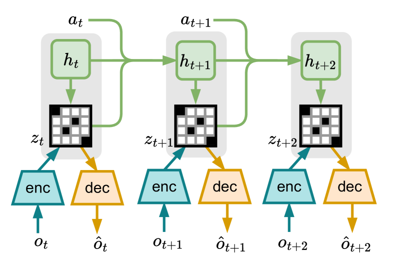
(a) World-Model Learning

(b) Actor-Critic Learning

(c) Extended Actor

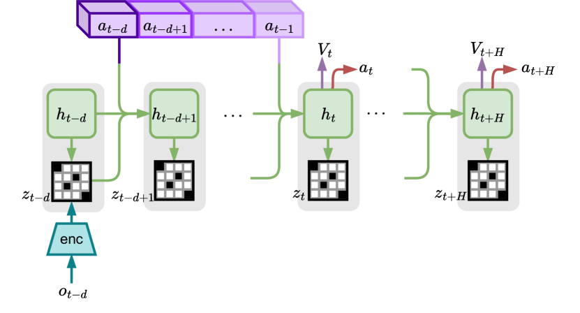
(d) Latent State Imagination

Figure 1: Panels (1(a)) and (1(b)) depict the standard Dreamer learning process, while (1(c)) and (1(d)) illustrate two strategies for adapting Dreamer model for observation delays.

3.1 Delayed POMDPs

A Partially Observable Markov Decision Process (POMDP) consists of a tuple $\langle\mathcal{S},\mathcal{A},\mathcal{T},\Omega,\mathcal{O},\gamma\rangle$, where $\mathcal{S}$ and $\mathcal{A}$ are the sets of states and actions, $\mathcal{T}(s^{\prime},r|s,a)$ is the joint probability distribution of the next state and reward, $\Omega$ is the set of observations, $\mathcal{O}(o|s^{\prime},a)$ is the conditional probability of observing $o\in\Omega$ after taking action $a$ and transitioning to state $s^{\prime}$, and $\gamma\in[0,1]$ is the discount factor. At each timestep $t$, the agent receives an observation $o_{t}$ and a reward $r_{t}$ from the environment, and the goal is to select actions $a_{t}$ to maximize the expected return $\mathbb{E}[\sum_{t\geq 0}\gamma^{t}r_{t}]$.

We formulate a Delayed POMDP (DPOMDP) as a tuple $\langle\mathcal{P}_{o},\mathcal{D}\rangle$ where $\mathcal{P}_{o}$ is a POMDP and $\mathcal{D}$ is a distribution generating the lag for receiving observations in $\mathcal{P}_{o}$. In other words, at time $t$, the agent receives observation $o_{t-d}$ and reward $r_{t-d}$, where $d\sim\mathcal{D}$. The goal is to maximize the expected return when behaving in $\mathcal{P}_{o}$ in the presence of delays. For simplicity, in this work we assume that $\mathcal{D}$ generates a constant non-negative integer delay $d$, but note that our methods are applicable to random delays as well.

In a similar fashion, delayed Markov Decision Processes (DMDPs) are defined in previous works (Wang et al., 2024; Liotet et al., 2022) as a tuple $\langle\mathcal{M},\mathcal{D}\rangle$, where $\mathcal{M}=\langle\mathcal{S},\mathcal{A},\mathcal{T},\gamma\rangle$ is an MDP. Like their undelayed counterparts, DMDPs can be considered a special case of DPOMDPs in which the (delayed) observation gives full information about the state at that time. Any DMDP can be reduced to an extended MDP $\widetilde{\mathcal{M}}$ by defining the states as a concatenation of the last observed state and the subsequent actions, which the agent needs to explicitly remember (Altman & Nain, 1992). In particular, $\widetilde{\mathcal{M}}=\langle\mathcal{X},\mathcal{A},\widetilde{\mathcal{T}},\gamma\rangle$, where $\mathcal{X}=\mathcal{S}\times\mathcal{A}^{d}$ and for $x=\left(s,a^{1},\ldots,a^{d}\right),x^{\prime}=\left(s^{\prime},a^{\prime 1},\ldots,a^{\prime d}\right)\in\mathcal{X}$,

$$\widetilde{\mathcal{T}}(x^{\prime},r|x,a)=\mathcal{T}(s^{\prime},r|s,a^{1})\mathbbm{1}([a^{\prime 1},\ldots,a^{\prime d}]=[a^{2},\ldots,a^{d},a]).$$ (1)

By definition, any DPOMDP is another POMDP with a specific structure. It can be formally constructed by defining the set of states in the new PODMP as the concatenation of the last $d+1$ states, of which only the earliest one is observable, and defining the transition probabilities accordingly. Thus, we can employ the POMDP framework to tackle the observation delays by constructing the equivalent POMDP (Varakantham & Marecki, 2012). On the other hand, one can exploit the structure introduced by delay in the process. Specifically, delays in receiving observations is equivalent to delay in inferring about the latent states. As latent space enjoys the Markov property, we can then work with the DMDP defined over latent states and induced by delay in observations. Note that there is a tradeoff between these two choices: on the one hand POMDPs are harder to learn; on the other hand, in the POMDP formulation, the world remembers the history for us, avoiding the curse of dimensionality in explicit agent context.

3.2 World models

World models (Schmidhuber, 2015; Ha & Schmidhuber, 2018) simulate aspects of the environment by learning an internal representation through an encoder and a dynamics model. The encoder compresses high-dimensional inputs, such as image observations, into a lower-dimensional embedding, while the dynamics model forecasts future states from historical information. This streamlined state representation then serves as input to an RL agent.

Dreamer (Hafner et al., 2020; 2021; 2023), a pioneering model-based RL (MBRL) approach utilizing world models, surpasses many model-free RL algorithms in data efficiency and performance. Particularly effective in visual control tasks with high-dimensional image observations, Dreamer trains agents with an imagined trajectories predicted by its world model. Dreamer’s training involves three alternating phases: 1) training the world model on past experiences; 2) learning behaviors with actor–critic algorithm through imagined sequences; and 3) collecting data in the environment.

Fig. 1(a) depicts the world model consisting of an encoder–decoder and a Recurrent State Space Model (RSSM) (Hafner et al., 2019) to model dynamics. Alongside observation reconstruction $\hat{o}_{t}$, it also has prediction heads for reward and episode continuation, which are omitted for clarity. The model state, $m_{t}=[h_{t},z_{t}]$, is composed of deterministic and stochastic components, respectively, given by

$$h_{t}=f_{\phi}(h_{t-1},z_{t-1},a_{t-1})$$ (2)

$$z_{t}\sim q_{\phi}(z_{t}|o_{t},h_{t}).$$ (3)

Dreamer also learns a dynamic predictor

$$z^{\prime}_{t}\sim p_{\phi}(z^{\prime}_{t}|h_{t})$$ (4)

for predicting imagined latent states.

As (2) and (3) suggest, the latent states are constructed to have a Markov structure, regardless of whether the observations themselves are Markov. In other words, Dreamer attempts to learn a latent-state MDP that is as nearly as possible equivalent to the observed POMDP. If it succeeds, this equivalence means that, for any policy $\pi(a|m)$, the stochastic process $\{m_{t},a_{t},r_{t}\}_{t\geq 0}$ induced by the policy in the world model (Figure 1(b)) has the same joint distribution as the embedding of real policy rollouts (Figure 1(a)). Figure 1(b) also illustrates Dreamer’s behavior learning using an actor–critic method, training policy and value heads on latent trajectories predicted by the world model.

3.3 Hardness of delayed control

Figure 2:

Before presenting our method, we provide an example to show that optimal values in DMDPs are generally incomparable for different delays. Depending on the stochasticity of the environment and the length of the delay, the optimal value function can be made arbitrary worse compared to that of the undelayed environment.

Let $V^{*}$ be the optimal value function of the MDP sketched in figure 2 and similarly $\widetilde{V}^{*}$ be the optimal value function with constant observation delays of $1$. Starting at state $s_{1}$, the agent will receive a reward of $+1$ for taking $a_{1}$ in $s_{1}$ and $0$ otherwise. Also, $0\leq\delta\leq\frac{1}{2}$ controls the stochasticity of the environment. To maximize the expected return, agent should stay in $s_{1}$ by taking $a_{1}$ in $s_{1}$ and $a_{2}$ in $s_{2}$. When there is no delay, the agent can take the appropriate action and avoid the absorbing state $s_{3}$. However, with delay, agent doesn’t observe the current state and for $0<\delta$ it eventually ends up in $s_{3}$ for any policy. The ratio between the optimal values of the delayed and undelayed case can be computed (see appendix A) as

$$\frac{\widetilde{V}^{*}(s_{1})}{V^{*}(s_{1})}=\frac{(1-\gamma)}{(1-\gamma\delta)\left(1-\gamma(1-\delta)\right)}.$$ (5)

When $\delta=0$ the ratio is 1, while the minimal ratio of $\frac{1-\gamma}{(1-\gamma/2)^{2}}$ is obtained for $\delta=\frac{1}{2}$ with the ratio approaching 0 as $\gamma\rightarrow 1$. These two extreme cases correspond to the scenarios with the least and the most stochasticity in the transitions, respectively.

In general, depending on the underlying MDP, even introducing small observation delays could downgrade the optimal policies by much. By assuming smooth transition dynamics and rewards, Liotet et al. (2022) bounded this gap as a function of smoothness parameters of the underlying MDP.

4 Delayed Control via World Models

In this section, we begin with a seemingly simple yet crucial insight into the relationship between converting POMDPs into MDPs via world models, and translating DPOMDPs into DMDPs. This insight forms the basis for combining techniques initially developed for POMDPs and DMDPs to tackle delays in partially observable environments. Next, we elaborate on the adaptations required to incorporate delays and examine two distinct methodologies within this framework.

4.1 World models reduce DPOMDPs to DMDPs

A world model $\widehat{M}$ is deemed equivalent to a POMDP $\mathcal{P}o$, if for any sequence $\{m_{t},a_{t},r_{t},o_{t}\}_{t\geq 0}$, the conditional probability $P(\{m_{t},r_{t}\}_{t\geq 0}|\{a_{t},o_{t}\}_{t\geq 0})$ remains identical when evaluated in both $\widehat{M}$ and $\mathcal{P}_{o}$.

Proposition 1.

If a world model $\widehat{M}$ is equivalent to a POMDP $\mathcal{P}_{o}$, then the $d$-step delayed world model $\widehat{M}^{d}$ is equivalent to the $d$-step delayed DPOMDP $\mathcal{P}_{o}^{d}$.

Proof.

For any action sequence $\vec{a}=\{a_{t}\}_{t\geq 0}$, consider the stochastic process $\widehat{\Xi}=\{\hat{\xi}_{t}=(m_{t},r_{t})\}_{t\geq 0}$ induced by rolling out $\vec{a}$ in $\widehat{M}$. Further consider the stochastic process $\Xi=\{\xi_{t}=(o_{t},m_{t},r_{t})\}_{t\geq 0}$ induced by rolling out $\vec{a}$ in $\mathcal{P}_{o}$, with $m_{t}$ sampled given $(o_{\leq t},a_{<t})$ by $\widehat{M}$’s stochastic encoder. Because $M$ and $\widehat{M}$ are equivalent, $\Xi$ (excluding $o_{t}$) and $\widehat{\Xi}$ have the same joint distribution. Proposition 1 then follows by noting that the delayed world model $\widehat{M}^{d}$ and the DPOMDP $\mathcal{P}_{o}^{d}$ respectively induce $\widehat{\Xi}^{d}=\{\hat{\xi_{t}}=(m_{t-d},r_{t-d})\}_{t\geq d}$ and $\Xi^{d}=\{\xi_{t}=(o_{t-d},m_{t-d},r_{t-d})\}_{t\geq d}$. Here, $m_{t-d}$ is embedded given $(o_{\leq t-d},a_{<t-d})$, despite subsequent actions being already available. It is straightforward to verify that these $d$-step delayed processes are likewise identically distributed, establishing the equivalence. ∎

Proposition 1 implies that we can use a world model with delayed observations to construct a delayed MDP in the latent space. This transition enables us to use latent extended state defined as $x_{t}=(m_{t-d},a_{t-d},...,a_{t-1})$, to tackle delays in POMDPs.

4.2 Delay-aware training

The learning of the world model itself relies on data stored in an experience replay buffer, which is accumulated by the agent throughout the training process. With delays, the storage of these data remains unaffected, as the data collection mechanism can store a transition once the subsequent observation becomes available and therefore, world model can be trained using undelayed data $\{(o_{t},a_{t},r_{t})\}_{t\geq 0}$. However, the distribution of collected samples is influenced by the fact that actions are selected without observing the current state of the environment. This discrepancy leads to a divergence in the distribution of data trajectories between the delayed and the undelayed enviornments. Nevertheless, as we will see in the experiment section, the world model can still learn successfully.

In contrast to world model learning, the actor–critic component must take delays into account, as the agent is required to select $a_{t}$ based on the available information at time $t-d$. To account for delayed observations, there are two primary design strategies: either to condition the policy directly on $x_{t}$, or predict the latent state $\hat{m}_{t}$ from $x_{t}$. In both cases, the agent needs access to the action sequences $(a_{t-d},...,a_{t-1})$. Thus, we augment the replay buffer to store subsequent actions. In the following two sections, we will explore each of these design approaches.

4.3 Delayed actor-critic

In actor–critic learning, the critic provides an estimate of the value function to aid the learning of the actor, while the actor aims to maximize the return guided by the critic’s value. For the actor, the extended state of the world model is sufficient to select $a_{t}$ given available information. The critic, in contrast, only provides feedback in training time and can therefore wait to see the true state to provide a more accurate value estimate to the actor. This idea has also been explored concurrently with this work (Wang et al., 2024). Thus, to account for observation delays, directly in the policy, we can use the extended state to design the policy network $\pi_{\theta}(a_{t}|x_{t})$ along with the same critic as in the undelayed case $V_{\psi}(m_{t})$. We refer to this method as an Extended actor. In practice, the policy can be implemented with any neural architecture, such as a Multi-Layer Perceptrons (MLP), Recurrent Neural Network (RNN), or Transformer.

Figure 1(c) illustrates the Extended actor diagram in the actor–critic learning phase of Dreamer. At time $t$, the agent retrieves $(x_{t},a_{t-d-1})$ from the replay buffer and performs actor–critic learning in imagination by updating the extended state with the next selected action. In particular, $a_{t}\sim\pi_{\theta}(a_{t}|x_{t})$ and $x_{t+1}=(m^{\prime}_{t-d+1},\{a_{i}\}_{i=t-d}^{t})$ where $m^{\prime}_{t-d+1}$ is the imagined latent state in 4. Note that critic predicts the value for the current latent state $V_{\psi}(m_{t-d})$ while the actor outputs $a_{t}$ based on the extended state. Thus, the imagination horizon will be increased for $d$ additional time steps since the critic provide feedback for actor’s action $d$ timesteps later. The estimates of the critic and the actions of the agent are then realigned to compute the policy gradient loss function.

Another variant of the extended actor involves drawing actions from the policy $\pi_{\theta}(a_{t}|m_{t-d})$ without maintaining a memory to track previously performed actions, a concept referred to as the Memoryless actor. While this design choice might appear to lack the ability to capture the necessary information, the rationale behind it is that the policy $\pi_{\theta}(a_{t}|m_{t-d})$ can theoretically represent previously performed actions within its network. This is because no new information is introduced after time $t-d$, and therefore, no additional memory is needed to store those actions.

4.4 Latent state imagination

Another approach to account for delays is to estimate the current latent state and use it in the actor. Specifically, we can use the world model’s forward dynamics in (2) and (4) (Figure 1(b)) for $d$ time steps, starting with the latest available latent state $m_{t-d}$, to sample a latent state prediction $\hat{m}_{t}$. Then, the agent uses $\hat{m}_{t}$ as the current latent state of the environment both in training and inference time. Figure 1(d) depicts this process, which we refer to as a Latent actor. After computing $\hat{m}_{t}$, the agent starts performs the actor–critic learning phase in Dreamer in training time, or uses the actor to select an action $a_{t}\sim\pi(a_{t}|\hat{m}_{t})$ during policy execution.

Note that estimation of the current state happens in the latent space, otherwise this approach will lead to sub-optimal decisions as the agent needs to form an approximate belief over the hidden state to act optimally in the presence of delays. In other words, the agent should account for uncertainty over the true state of the environment. This also implies that the latent state should have a non-stochastic part to allow the agent not to lose information by sampling.

5 Experiments

5.1 Experimental setup

Tasks.

To evaluate our proposed methods, we conducted experiments across a diverse set of environments. We have considered four continuous control tasks from MuJoCo (Todorov et al., 2012) in Gymnasium (Gym) (Towers et al., 2023): HalfCheetah-v4, HumanoidStandup-v4, Reacher-v4, and Swimmer-v4 for comparison with previous studies. Also, we extended our evaluation to six more environments from the DeepMind Control Suite (DMC) (Tunyasuvunakool et al., 2020), to further examine our methods with both proprioceptive and visual observations. The distinction between these input types is critical; vector inputs provide a fully observable state of the environment. However image-based observations introduce partial observability, necessitating approaches capable of addressing delays within the POMDP framework.

Methods.

We utilized Dreamer-V3 (Hafner et al., 2023) as our primary framework and compare with prior studies, including D-TRPO (Liotet et al., 2021) and DC-AC (Bouteiller et al., 2020). We also evaluated a Dreamer-V3 agent, similar to the Latent method, except trained in an undelayed setting and tested under delayed conditions with latent imagination. We refer to this approach as the Agnostic Dreamer, which could be thought of naively using Dreamer to address delays. Although our methods can handle both constant and random delays, we chose to focus on fixed delays for simplicity and comparability with the baselines. While we experiment in both Gym and DMC, the baselines were originally designed and tuned for Gym environments with vector inputs, and we found the task of modifying them for image observations or tuning their hyperparameters for DMC nontrivial (Cetin et al., 2022) and thus outside our scope. Also, for Gym environments, we trained Dreamer variants with a budget of $500$K interactions, while D-TRPO and DC-AC trained with $5$M and $1$M environment interactions. For DMC tasks with visual inputs, we have increased the number of interactions to $1$M.

Architectures and hyperparameters.

For D-TRPO, we adopted the hyperparameters and architecture detailed in Liotet et al. (2022). Similarly, for DC-AC, we replicated the hyperparameters and model from the original paper (Bouteiller et al., 2020). In our delayed variants of Dreamer-V3, we maintained consistency by using the same set of hyperparameters and architecture as the original implementation (Hafner et al., 2023). The only architectural adjustment was for the extended agent, where we incorporated a Multi-Layer Perceptron (MLP) for the policy network to extend the latent state with actions. Note that while we used the same set of hyperparameters provided in the original dreamer, we conjecture that the optimal horizon length should be smaller in both the Extended and Latent methods, where the effective horizon is longer due to the action buffer (Figures 1(c) and 1(d)), because accumulation of one-step errors in imagination via forward dynamics could harm the actor-critic learning part. Each experiment has been repeated with $3$ random seeds.

Note that, in all experiments, the agent will perform random actions until the first observation becomes available. While one could utilize better strategies for initial actions, using random actions is common in all existing delayed RL methods.

5.2 Results

(a) HalfCheetah-v4

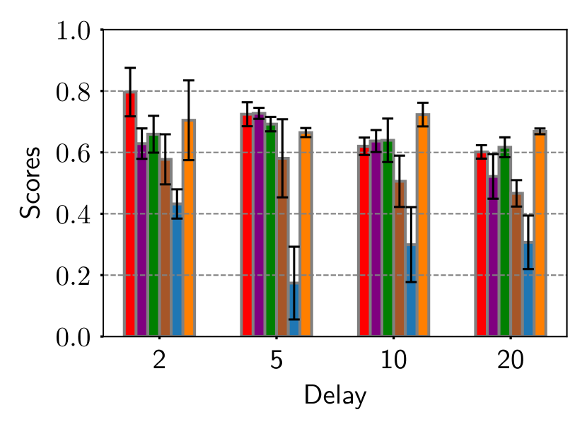
(b) HumanoidStandup-v4

(c) Reacher-v4

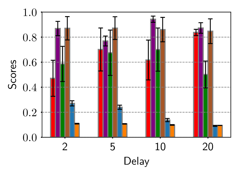
(d) Swimmer-v4

(e) DMC proprio

(f) DMC vision

Figure 3: Normalized returns across different environments for varying delays. Bars and caps represent the mean and standard error of the mean, respectively. Panels (3(e)) and (3(f)) are averaged over the selected suites in DMC, after normalizing standard Dreamer-V3 in the undelayed environment to 1 and the random policy to 0.

Figures 3(a)–3(d) depict the results obtained from the experiments conducted on the selected Gym environments. The Dreamer variants demonstrate a significant performance improvement over D-TRPO across all tasks. However, DC-AC exhibits comparable performance to our methods on HalfCheetah-v4 and HumanoidStandup-v4, outperforms them on Reacher-v4, and underperforms on Swimmer-v4. One reason that why our methods are not performing well on Reacher-v4, could be due to the perofrmance of the standard Dreamer, trained and tested on the undelayed environment itself. This is evident as DC-AC achieves comparable or superior performance to the standard Dreamer on these environments with small delays. One potential explanation for this phenomenon could be the significant portion of samples in actor–critic learning that fall outside the planning horizon. This is likely due to our use of the same imagination horizon length $H=16$ and an episode length of $50$ for this task.

Figures 3(e) and 3(f) display the performance of our methods averaged over selected suites in DMC with proprioceptive and image inputs, respectively. Remarkably, the Agnostic method performs very well across all tasks without knowing about the delay in training time. Also, the Agnostic method needs not know the delay distribution beforehand and can be deployed on any delayed environment. However, as delay increases the performance drops more rapidly than for other methods. This is because the distribution shift between the undelayed training and delayed evaluation increases for larger delays. Similarly, the Latent method does not exhibit robustness against long delays, as Dreamer employs one-step prediction to roll out the world model. The accumulation of one-step prediction errors over longer delays causes the predicted latent state to diverge significantly from the true latent state. As expected, Extended proves to be the most robust among our variants, as it utilizes next actions and avoids the accumulation of errors present in Latent and Agnostic. Notably, Extended improves by $30\%$ on average in DMC vision tasks compared to Agnostic.

Additionally, we include training curves and tables summarizing the final test performance for all tasks in Appendix B.

5.3 Degree of observability

Figure 4 illustrates the resilience of the Extended and the baselines facing with increasing level of partial observability in HalfCheetah-v4 environment. Originally, the environment’s observations encompass both the positional and velocity information for the agent’s joints. To simulate partial observability, we modified the environment to omit a $\rho$ percentage of the velocity components. The results demonstrate that both the Extended and D-TRPO were capable of inferring the missing velocity components from historical observations. Although D-TRPO is specifically designed for delays in MDPs, in this particular scenario, it was able to compute the relative velocities by utilizing a transformer used to process the extended state. In contrast, DC-AC deteriorated significantly as environments became less observable.

Figure 4: Return against the degree of observability in HalfCheeth-v4 for $d=5$.

6 Conclusion

In this paper, we have proposed using world models for delayed observation within the POMDP framework. To showcase our methods, we adapted Dreamer-V3 for delay in observations and proposed two strategies, one using a delayed actor and the other latent state imagination. We discussed another version of the delayed actor which operates without action memory and additionally introduced a delay-agnostic strategy which needs not know the delay distribution beforehand. Evaluation revealed that our methods are robust to partial observability of the environment and can outperform the baselines in overall, but show comparable or worse performance in cases where their untuned hyperparameters are inappropriate.

Our experiments revealed that for small delays, Memoryless and Latent approach work the best while keeping the original model the same. However, as delay gets larger they fall short to maintain their performance due to the lack of action memory and accumulation of one-step errors issues. But Extended method can maintain its performance with the expense of adding more complexity to the initial model.

Appendix A MDP example

The optimal policy will select $a_{1}$ in $s_{1}$ and $a_{2}$ in $s_{2}$. Then, by Bellman optimal equation for the state-value function we have

$$V^{*}(s_{1})=1+\gamma(1-\delta)V^{*}(s_{1})+\gamma\delta V^{*}(s_{2})$$ (6)

$$V^{*}(s_{2})=\gamma(1-\delta)V^{*}(s_{1})+\gamma\delta V^{*}(s_{2}),$$ (7)

which yields $V^{*}(s_{1})=\frac{1-\gamma\delta}{1-\gamma}$. In the case of observation delay with $d=1$, the optimal policy will select $a_{1}$ in every state since $\frac{1}{2}\leq\delta$ and thus,

$$\widetilde{V}^{*}(x_{1})=(1-\delta)\left(1+\gamma\widetilde{V}^{*}(x_{1})\right),$$ (8)

where $x_{1}$ is the extended state $(s_{1},a_{1})$. For the current state of the environment in $s_{1}$, we have $\widetilde{V}^{*}(s_{1})=1+\gamma\widetilde{V}^{*}(x_{1})$. Therefore, $\widetilde{V}^{*}(s_{1})=\frac{1}{1-\gamma(1-\delta)}$.

Appendix B Experiment Details

In this section, we have included the training curves and the final results of our experiments across the selected environments in Gym and DMC. In order to have a fair comparison between the methods, we have used the same random seed for generating random actions at the begining of the episode. We refer to DMC tasks with proprioceptive and image observations as DMC proprio and vision, respectively.

B.1 Gym results

Task	Delay	Extended Dreamer	Memoryless Dreamer	Latent Dreamer	Agnostic Dreamer	D-TRPO	DC-AC
HalfCheetah-v4 ($\times 10^{3}$)	2	$5.09\pm 0.443$	$4.46\pm 0.821$	$3.15\pm 0.916$	$3.38\pm 0.492$	$1.91\pm 0.189$	$\mathbf{7.82\pm 0.260}$
	5	$3.32\pm 0.853$	$3.30\pm 0.814$	$1.85\pm 0.242$	$1.29\pm 0.375$	$1.47\pm 0.018$	$\mathbf{3.48\pm 0.955}$
	10	$\mathbf{3.56\pm 0.644}$	$3.03\pm 0.178$	$1.21\pm 0.180$	$0.427\pm 0.199$	$1.50\pm 0.087$	$2.35\pm 0.413$
	20	$1.66\pm 0.261$	$\mathbf{2.41\pm 0.552}$	$0.732\pm 0.254$	$0.160\pm 0.028$	$1.45\pm 0.374$	$0.659\pm 0.347$
HumanoidStandup-v4 ($\times 10^{5}$)	2	$\mathbf{1.76\pm 0.142}$	$1.52\pm 0.108$	$1.46\pm 0.089$	$1.37\pm 0.147$	$1.11\pm 0.086$	$1.60\pm 0.234$
	5	$\mathbf{1.64\pm 0.071}$	$1.57\pm 0.042$	$1.63\pm 0.033$	$1.37\pm 0.230$	$0.640\pm 0.214$	$1.52\pm 0.027$
	10	$1.44\pm.05$	$1.47\pm 0.12$	$1.47\pm 0.06$	$1.23\pm 0.15$	$0.86\pm 0.22.0$	$\mathbf{1.63\pm 0.69}$
	20	$1.41\pm 0.039$	$1.44\pm 0.059$	$1.27\pm 0.132$	$1.17\pm 0.078$	$0.880\pm 0.157$	$\mathbf{1.53\pm 0.017}$
Reacher-v4	2	$-8.2\pm 1.1$	$-7.1\pm 0.6$	$-8.2\pm 0.8$	$-9.4\pm 0.1$	$-12.9\pm 1.1$	$\mathbf{-4.6\pm 0.0}$
	5	$-11.6\pm 0.5$	$-10.7\pm 0.1$	$-11.7\pm 1.1$	$-11.5\pm 0.4$	$-12.9\pm 0.8$	$\mathbf{-4.8\pm 0.1}$
	10	$-15.5\pm 0.2$	$-16.4\pm 1.5$	$-14.8\pm 1.5$	$-15.3\pm 0.3$	$-15.6\pm 0.9$	$\mathbf{-5.3\pm 0.1}$
	20	$-24.3\pm 0.6$	$-26.1\pm 0.5$	$-23.9\pm 0.5$	$-23.1\pm 0.2$	$-23.3\pm 0.4$	$\mathbf{-7.2\pm 0.2}$
Swimmer-v4	2	$167.5\pm 49.9$	$207.3\pm 48.6$	$\mathbf{305.2\pm 19.7}$	$305.0\pm 20.8$	$98.3\pm 7.1$	$42.1\pm 1.0$
	5	$247.2\pm 59.4$	$238.2\pm 62.7$	$270.7\pm 13.7$	$\mathbf{305.7\pm 20.0}$	$87.5\pm 5.7$	$41.5\pm 0.7$
	10	$218.1\pm 55.1$	$246.9\pm 59.7$	$\mathbf{330.9\pm 8.6}$	$302.4\pm 21.4$	$52.1\pm 4.4$	$38.6\pm 0.9$
	20	$294.4\pm 8.6$	$178.2\pm 37.1$	$\mathbf{306.7\pm 14.6}$	$297.7\pm 18.3$	$59.2\pm 6.8$	$36.9\pm 0.8$

Table 1: Final test returns on tasks in Gym. Results are presented as the mean $\pm$ standard error of the mean.

B.2 DMC proprio results

Task	Delay	Extended Dreamer	Memoryless Dreamer	Latent Dreamer	Agnostic Dreamer
Acrobot Swingup	2	$232.6\pm 13.2$	$244.3\pm 45.7$	$237.6\pm 22.6$	$\mathbf{256.6\pm 22.9}$
	5	$219.5\pm 74.6$	$228.7\pm 16.3$	$\mathbf{251.6\pm 38.5}$	$240.9\pm 13.1$
	10	$109.1\pm 19.1$	$161.0\pm 27.3$	$185.9\pm 10.9$	$\mathbf{197.0\pm 17.0}$
	20	$61.9\pm 19.5$	$85.4\pm 22.2$	$\mathbf{148.0\pm 11.4}$	$129.7\pm 11.3$
Cartpole Balance	2	$983.2\pm 6.5$	$\mathbf{993.0\pm 0.2}$	$990.2\pm 1.6$	$992.4\pm 2.4$
	5	$989.2\pm 1.2$	$984.7\pm 2.8$	$983.1\pm 6.6$	$\mathbf{990.0\pm 3.4}$
	10	$962.1\pm 5.5$	$935.9\pm 17.3$	$885.2\pm 81.5$	$\mathbf{980.4\pm 2.1}$
	20	$\mathbf{831.4\pm 23.6}$	$652.1\pm 18.0$	$738.1\pm 34.3$	$511.9\pm 32.8$
Cheetah Run	2	$604.3\pm 33.3$	$\mathbf{695.6\pm 22.3}$	$687.1\pm 34.5$	$596.1\pm 72.8$
	5	$596.4\pm 44.9$	$\mathbf{648.4\pm 11.8}$	$512.3\pm 58.9$	$373.2\pm 39.5$
	10	$444.6\pm 25.5$	$\mathbf{503.6\pm 8.0}$	$312.8\pm 79.3$	$173.6\pm 20.6$
	20	$\mathbf{418.7\pm 30.6}$	$329.0\pm 22.2$	$199.6\pm 19.8$	$119.7\pm 3.4$
Finger Spin	2	$527.6\pm 27.4$	$427.3\pm 27.9$	$247.0\pm 123.2$	$\mathbf{561.1\pm 93.5}$
	5	$283.6\pm 14.8$	$271.1\pm 11.6$	$\mathbf{361.1\pm 86.3}$	$278.3\pm 31.1$
	10	$\mathbf{287.4\pm 35.7}$	$161.9\pm 15.5$	$159.2\pm 26.6$	$111.1\pm 7.5$
	20	$\mathbf{177.8\pm 23.8}$	$116.9\pm 7.7$	$129.8\pm 12.3$	$59.5\pm 8.1$
Hopper Hop	2	$93.8\pm 33.8$	$143.0\pm 23.5$	$\mathbf{176.7\pm 34.8}$	$121.0\pm 11.9$
	5	$127.4\pm 11.4$	$\mathbf{171.4\pm 31.2}$	$58.5\pm 16.3$	$53.6\pm 6.2$
	10	$\mathbf{111.1\pm 29.8}$	$66.7\pm 27.0$	$35.5\pm 15.4$	$20.0\pm 4.7$
	20	$\mathbf{22.9\pm 22.9}$	$0.0\pm 0.0$	$5.5\pm 1.6$	$11.1\pm 3.6$
Walker Walk	2	$883.9\pm 22.1$	$\mathbf{924.0\pm 4.5}$	$917.7\pm 19.3$	$732.5\pm 39.1$
	5	$\mathbf{793.6\pm 86.2}$	$592.3\pm 69.7$	$554.2\pm 29.5$	$389.5\pm 18.0$
	10	$\mathbf{566.8\pm 6.8}$	$530.2\pm 22.2$	$328.4\pm 23.5$	$219.4\pm 5.5$
	20	$\mathbf{391.3\pm 27.5}$	$389.1\pm 19.4$	$170.6\pm 13.0$	$170.3\pm 0.2$

Table 2: Final test returns on tasks in DMC with proprioceptive inputs. Results are presented as the mean $\pm$ standard error of the mean.

B.3 DMC vision results

Task	Delay	Extended Dreamer	Memoryless Dreamer	Latent Dreamer	Agnostic Dreamer
Acrobot Swingup	2	$289.3\pm 49.3$	$355.6\pm 50.1$	$\mathbf{428.8\pm 17.9}$	$396.3\pm 67.3$
	5	$326.3\pm 12.0$	$286.1\pm 29.8$	$342.3\pm 44.3$	$\mathbf{382.6\pm 28.5}$
	10	$279.4\pm 21.1$	$191.2\pm 30.5$	$\mathbf{338.9\pm 34.5}$	$326.0\pm 49.3$
	20	$133.2\pm 12.6$	$116.0\pm 37.6$	$\mathbf{263.8\pm 27.8}$	$230.4\pm 16.5$
Cartpole Balance	2	$995.8\pm 0.3$	$996.0\pm 0.2$	$\mathbf{996.3\pm 0.1}$	$\mathbf{996.3\pm 0.1}$
	5	$994.7\pm 0.1$	$993.0\pm 0.1$	$994.6\pm 0.8$	$\mathbf{995.2\pm 0.1}$
	10	$979.2\pm 6.5$	$950.3\pm 22.3$	$\mathbf{980.2\pm 8.2}$	$926.0\pm 60.7$
	20	$928.4\pm 14.7$	$677.4\pm 4.5$	$\mathbf{933.1\pm 15.0}$	$570.8\pm 27.0$
Cheetah Run	2	$\mathbf{872.3\pm 10.6}$	$815.0\pm 44.5$	$872.0\pm 7.2$	$799.1\pm 32.0$
	5	$\mathbf{840.7\pm 10.3}$	$805.4\pm 11.3$	$751.1\pm 72.1$	$533.1\pm 37.3$
	10	$\mathbf{618.8\pm 55.2}$	$603.7\pm 28.8$	$538.5\pm 43.0$	$251.2\pm 49.5$
	20	$\mathbf{499.7\pm 31.8}$	$369.7\pm 22.0$	$254.5\pm 32.8$	$118.8\pm 11.4$
Finger Spin	2	$496.3\pm 118.3$	$403.6\pm 42.9$	$\mathbf{575.7\pm 179.0}$	$418.0\pm 211.1$
	5	$\mathbf{359.6\pm 10.8}$	$343.7\pm 11.7$	$290.7\pm 34.9$	$254.4\pm 128.8$
	10	$\mathbf{266.3\pm 34.7}$	$179.8\pm 9.5$	$88.2\pm 51.1$	$99.7\pm 50.1$
	20	$\mathbf{177.9\pm 18.6}$	$107.3\pm 6.1$	$55.5\pm 33.8$	$49.3\pm 24.2$
Hopper Hop	2	$288.6\pm 37.4$	$309.0\pm 33.0$	$\mathbf{357.5\pm 64.1}$	$64.0\pm 64.0$
	5	$\mathbf{203.7\pm 14.5}$	$195.4\pm 13.6$	$140.0\pm 35.8$	$18.0\pm 17.8$
	10	$132.9\pm 9.4$	$\mathbf{138.4\pm 20.0}$	$31.0\pm 6.4$	$3.5\pm 3.5$
	20	$\mathbf{142.6\pm 12.8}$	$22.8\pm 21.5$	$3.8\pm 2.1$	$2.3\pm 2.3$
Walker Walk	2	$938.7\pm 7.3$	$921.3\pm 18.5$	$\mathbf{951.4\pm 12.2}$	$916.0\pm 12.8$
	5	$749.4\pm 76.1$	$\mathbf{871.2\pm 20.1}$	$740.9\pm 30.8$	$524.4\pm 35.6$
	10	$\mathbf{566.8\pm 6.8}$	$530.2\pm 22.2$	$328.4\pm 23.5$	$219.4\pm 5.5$
	20	$\mathbf{477.3\pm 67.8}$	$363.5\pm 57.5$	$164.6\pm 2.8$	$147.3\pm 11.2$

Table 3: Final test returns on tasks in DMC with visual inputs. Results are presented as the mean $\pm$ standard error of the mean.

B.4 Gym training curves

Figure 5: Training curves for the set of tasks in Gym. Dreamer variants trained with 500K interactions of the environment, while D-TRPO and DC-AC used 5M and 1M interactions, respectively. For D-TRPO and DC-AC, we have plotted the final training performance.

B.5 DMC proprio training curves

Figure 6: Training curves for the set of tasks in DMC with proprioceptive inputs with 500K interactions.

B.6 DMC vision training curves

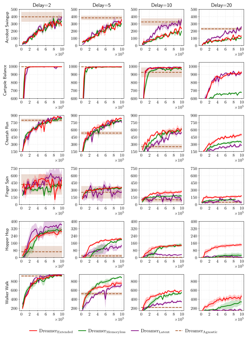
Figure 7: Training curves for the set of tasks in DMC with visual inputs with 1M interactions.

References

- Almutairi et al. (2022) Jaber Almutairi, Mohammad Aldossary, Hatem A Alharbi, Barzan A Yosuf, and Jaafar MH Elmirghani. Delay-optimal task offloading for uav-enabled edge-cloud computing systems. IEEE Access, 10:51575–51586, 2022.
- Altman & Nain (1992) Eitan Altman and Philippe Nain. Closed-loop control with delayed information. ACM sigmetrics performance evaluation review, 20(1):193–204, 1992.
- Bouteiller et al. (2020) Yann Bouteiller, Simon Ramstedt, Giovanni Beltrame, Christopher Pal, and Jonathan Binas. Reinforcement learning with random delays. In International conference on learning representations, 2020.
- Cetin et al. (2022) Edoardo Cetin, Philip J Ball, Steve Roberts, and Oya Celiktutan. Stabilizing off-policy deep reinforcement learning from pixels. In International Conference on Machine Learning, 2022.
- Chen et al. (2021) Baiming Chen, Mengdi Xu, Liang Li, and Ding Zhao. Delay-aware model-based reinforcement learning for continuous control. Neurocomputing, 450:119–128, 2021.
- Derman et al. (2020) Esther Derman, Gal Dalal, and Shie Mannor. Acting in delayed environments with non-stationary markov policies. In International Conference on Learning Representations, 2020.
- Dulac-Arnold et al. (2019) Gabriel Dulac-Arnold, Daniel Mankowitz, and Todd Hester. Challenges of real-world reinforcement learning. arXiv preprint arXiv:1904.12901, 2019.
- Ge et al. (2013) Yuan Ge, Qigong Chen, Ming Jiang, and Yiqing Huang. Modeling of random delays in networked control systems. Journal of Control Science and Engineering, 2013:8–8, 2013.
- Ha & Schmidhuber (2018) David Ha and Jürgen Schmidhuber. World models. arXiv preprint arXiv:1803.10122, 2018.
- Haarnoja et al. (2018) Tuomas Haarnoja, Aurick Zhou, Pieter Abbeel, and Sergey Levine. Soft actor-critic: Off-policy maximum entropy deep reinforcement learning with a stochastic actor. In International conference on machine learning, pp. 1861–1870. PMLR, 2018.
- Hafner et al. (2019) Danijar Hafner, Timothy Lillicrap, Ian Fischer, Ruben Villegas, David Ha, Honglak Lee, and James Davidson. Learning latent dynamics for planning from pixels. In International Conference on Machine Learning, pp. 2555–2565. PMLR, 2019.
- Hafner et al. (2020) Danijar Hafner, Timothy Lillicrap, Jimmy Ba, and Mohammad Norouzi. Dream to control: Learning behaviors by latent imagination. In International Conference on Learning Representations, 2020.
- Hafner et al. (2021) Danijar Hafner, Timothy Lillicrap, Mohammad Norouzi, and Jimmy Ba. Mastering atari with discrete world models. In International Conference on Learning Representations, 2021.
- Hafner et al. (2023) Danijar Hafner, Jurgis Pasukonis, Jimmy Ba, and Timothy Lillicrap. Mastering diverse domains through world models. arXiv preprint arXiv:2301.04104, 2023.
- Imaida et al. (2004) Takashi Imaida, Yasuyoshi Yokokohji, Toshitsugu Doi, Mitsushige Oda, and Tsuneo Yoshikawa. Ground-space bilateral teleoperation of ets-vii robot arm by direct bilateral coupling under 7-s time delay condition. IEEE Transactions on Robotics and Automation, 20(3):499–511, 2004.
- Katsikopoulos & Engelbrecht (2003) Konstantinos V Katsikopoulos and Sascha E Engelbrecht. Markov decision processes with delays and asynchronous cost collection. IEEE transactions on automatic control, 48(4):568–574, 2003.
- Kim & Jeong (1987) Soung Hie Kim and Byung Ho Jeong. A partially observable markov decision process with lagged information. Journal of the Operational Research Society, 38:439–446, 1987.
- Liotet et al. (2021) Pierre Liotet, Erick Venneri, and Marcello Restelli. Learning a belief representation for delayed reinforcement learning. In 2021 International Joint Conference on Neural Networks (IJCNN), pp. 1–8. IEEE, 2021.
- Liotet et al. (2022) Pierre Liotet, Davide Maran, Lorenzo Bisi, and Marcello Restelli. Delayed reinforcement learning by imitation. In International Conference on Machine Learning, pp. 13528–13556. PMLR, 2022.
- Mahmood et al. (2018) A Rupam Mahmood, Dmytro Korenkevych, Gautham Vasan, William Ma, and James Bergstra. Benchmarking reinforcement learning algorithms on real-world robots. In Conference on robot learning, pp. 561–591. PMLR, 2018.
- Schmidhuber (2015) Jürgen Schmidhuber. On learning to think: Algorithmic information theory for novel combinations of reinforcement learning controllers and recurrent neural world models. arXiv preprint arXiv:1511.09249, 2015.
- Schuitema et al. (2010) Erik Schuitema, Lucian Buşoniu, Robert Babuška, and Pieter Jonker. Control delay in reinforcement learning for real-time dynamic systems: A memoryless approach. In 2010 IEEE/RSJ International Conference on Intelligent Robots and Systems, pp. 3226–3231. IEEE, 2010.
- Sutton & Barto (2018) Richard S Sutton and Andrew G Barto. Reinforcement learning: An introduction. MIT press, 2018.
- Todorov et al. (2012) Emanuel Todorov, Tom Erez, and Yuval Tassa. Mujoco: A physics engine for model-based control. In 2012 IEEE/RSJ International Conference on Intelligent Robots and Systems, pp. 5026–5033. IEEE, 2012. doi: 10.1109/IROS.2012.6386109.
- Towers et al. (2023) Mark Towers, Jordan K. Terry, Ariel Kwiatkowski, John U. Balis, Gianluca de Cola, Tristan Deleu, Manuel Goulão, Andreas Kallinteris, Arjun KG, Markus Krimmel, Rodrigo Perez-Vicente, Andrea Pierré, Sander Schulhoff, Jun Jet Tai, Andrew Tan Jin Shen, and Omar G. Younis. Gymnasium, March 2023. URL https://zenodo.org/record/8127025.
- Tunyasuvunakool et al. (2020) Saran Tunyasuvunakool, Alistair Muldal, Yotam Doron, Siqi Liu, Steven Bohez, Josh Merel, Tom Erez, Timothy Lillicrap, Nicolas Heess, and Yuval Tassa. dm_control: Software and tasks for continuous control. Software Impacts, 6:100022, 2020. ISSN 2665-9638. doi: https://doi.org/10.1016/j.simpa.2020.100022. URL https://www.sciencedirect.com/science/article/pii/S2665963820300099.
- Varakantham & Marecki (2012) Pradeep Varakantham and Janusz Marecki. Delayed observation planning in partially observable domains. In Proceedings of the 11th International Conference on Autonomous Agents and Multiagent Systems-Volume 3, pp. 1235–1236, 2012.
- Walsh et al. (2007) Thomas J Walsh, Ali Nouri, Lihong Li, and Michael L Littman. Planning and learning in environments with delayed feedback. In Machine Learning: ECML 2007: 18th European Conference on Machine Learning, Warsaw, Poland, September 17-21, 2007. Proceedings 18, pp. 442–453. Springer, 2007.
- Walsh et al. (2009) Thomas J Walsh, Ali Nouri, Lihong Li, and Michael L Littman. Learning and planning in environments with delayed feedback. Autonomous Agents and Multi-Agent Systems, 18:83–105, 2009.
- Wang et al. (2024) Wei Wang, Dongqi Han, Xufang Luo, and Dongsheng Li. Addressing signal delay in deep reinforcement learning. In International Conference on Learning Representations, 2024. URL https://openreview.net/forum?id=Z8UfDs4J46.