Anomaly Induced Supernovae Cooling: New Contribution from Axions

Abstract

Compact stellar objects like supernovae and neutron stars are believed to cool by emitting axions predominantly via axion bremsstrahlung ($NN\to NNa$), pion conversion ($\pi^{-}p^{+}\to Na$) and photo-production ($\gamma N\to Na$). In this letter, we study a previously overlooked contribution to the photo-production channel, originating from the unavoidable anomaly-induced Wess-Zumino-Witten term $\propto\epsilon^{\mu\nu\alpha\beta}\,F_{\mu\nu}\,\partial_{\alpha}a\,\omega_{\beta}$. As a result, supernovae can cool up to three times faster than what was previously thought, translating into stronger bounds on the axion decay constant. Furthermore, the spectrum of axions emitted in the process is unique as it is significantly harder than those originating from bremsstrahlung. As a consequence, we find that these axions are more likely to show up in near future water Cherenkov detectors as compared to traditional ones.

Introduction.– Searches for new physics much lighter than the electroweak scale have gained a lot of attention in the recent past. Among all the possible candidates, axions or axion-like particles are perhaps the most well-motivated. Axion emerges as the pseudo-Nambu-Goldstone boson of a spontaneously broken $U(1)$ symmetry [1, 2, 3, 4] and offers a compelling solution to the long-standing strong-$CP$ problem [5] of the Standard Model (SM). Moreover, axions can also be a natural dark matter candidate [6, 7, 8], address the hierarchy problem [9, 10, 11] and play a crucial role in resolving the matter-antimatter asymmetry [12, 13] of the Universe. Naturally, axion furnishes complementary means to probe physics beyond the SM at multiple frontiers.

While the axion can have a myriad of couplings with the SM particles, the most minimal effective Lagrangian addressing the strong $CP$ problem, up to terms required for renormalization is given as:

$$\mathcal{L}=\mathcal{L}_{\text{SM}}+\frac{\alpha_{s}}{8\pi}\frac{a}{f_{a}}G\widetilde{G}+\frac{1}{2}\left(\partial_{\mu}a\right)^{2}-\frac{1}{2}m_{a_{0}}^{2}a^{2}\;,$$ (1)

where $G$ is the field strength tensor of the gluon and $a$ is the axion with decay constant $f_{a}$. For lighter axions, $m_{a}\lesssim\mathcal{O}(\text{GeV})$, it is convenient to rotate away the $aG\widetilde{G}$ coupling by a chiral transformation of the SM quark fields. The ensuing Lagrangian generates axion-quark kinetic and mass mixing terms and can be matched with an effective theory such as Chiral perturbation theory ($\chi$PT) containing mesons. This effective description provides a powerful framework to study non-perturbative effects such as axion-pion mixing and has been used to constrain large parts of axion parameter space from intensity frontier experiments such as beam dump [14, 15, 16], rare decays of pions [17, 18, 19] and kaons [20, 21, 22, 23, 24, 25, 26, 27], etc. However, for heavy QCD axions, $m_{a}\gtrsim\mathcal{O}(1)$ GeV, the power counting of $\chi$PT breaks down and one generally relies on pertubative computations to probe axions [28, 29, 30, 31], mostly from rare $B$-decays.

On the other hand, cosmic frontier provides complementary means to probe axions as it is sensitive to lighter masses, e.g., $m_{a}\lesssim\mathcal{O}(10)$ MeV. For example, nuclear reactions or thermal processes inside the stellar interior such as White Dwarf (WD), Neutron Star (NS), Supernova (SN), etc., are potentially powerful sources of axions. The emission of axions from such compact stellar objects might result in a more efficient transport of energy compared to the SM neutrinos, leading to observational changes. This lead the authors of Ref. [32, 33] to propose the following bound on the emissivity of axions

$${}\frac{Q_{a}}{\rho}\lesssim 10^{19}\;\text{erg}\;s^{-1}g^{-1}\;,$$ (2)

evaluated at a temperature $T=30-40$ MeV and around the nuclear saturation density. Traditionally, axion bremsstrahlung, i.e., $NN\to NNa$ [34, 35], where $N=(p,n)$ is a nucleon, was considered to be the most dominant channel of axion production in the core of the SN. Although previous studies assumed One Pion Exchange (OPE) approximation, large suppression was found while going beyond OPE [36]. Nevertheless, using Eq.(2), earlier bounds were drawn on the axion mass and effective axion-nucleon coupling [37, 38, 39, 40, 41, 42]. More recently, it was argued that pion conversion [43, 44] could potentially enhance the emissivity by a factor of few [45, 46], so is the existence of quark matter in the core of the SN [47]. We summarize those contributions and the relevant operators in Table 1.

Process	Coupling	Refs
$NN\to NNa$	$\left(C_{aN}/2f_{a}\right)\;\bar{N}\gamma_{5}\gamma_{\mu}N\;\partial^{\mu}a$	[34, 35]
$\pi^{-}p\to Na$	$\left(C_{aN}/2f_{a}\right)\;\bar{N}\gamma_{5}\gamma_{\mu}N\;\partial^{\mu}a$	[40, 45]
$N\gamma\to Na$	$i\;\left(C_{aN\gamma}/2\right)a\;\bar{N}\gamma_{5}\sigma_{\mu\nu}N\;F^{\mu\nu}$	[48, 49]
$N\gamma\to Na$	$\left(\kappa/f_{a}\right)\epsilon^{\mu\nu\rho\sigma}\;F_{\mu\nu}\;\partial_{\rho}a\;\omega_{\sigma}$	This work

Table 1: Interactions relevant for axion emission from a supernova. The coefficient $\kappa$ has been defined in Eq. (6).

In this minimal scenario, it is natural to ask whether there exists any other unavoidable interactions of axions or not. For example, in the SM, there exists Wess-Zumino-Witten (WZW) interactions [50, 51, 52, 53, 54, 55, 56, 57, 58, 59] which can account for certain processes including anomalies that can not be generated in $\chi$PT. This is because low-energy effective theories such as $\chi$PT can often possess more symmetries such as spurious parity than its UV counterpart QCD. Interestingly, in the presence of background gauge fields (such as $\omega$, $\rho$ mesons, etc.), the physics of WZW interactions are quite rich [57]. Recently it was shown that even in SM, such interactions open up new channels for the cooling of young neutron stars [56, 59]. In this Letter, we study the implications of WZW terms in the presence of axions leading to novel interactions.

WZW interactions.– To generate WZW interactions, one considers the 5-dimensional action [50, 51] which is invariant under chiral symmetry, where the boundary is identified with our 4-dimensional spacetime, e.g.,

$$S_{\rm WZW}(A_{\mu},U)=N_{c}\int_{D}\;d^{5}y\;\omega\;,$$

$$\omega=-\frac{i}{240\pi^{2}}\;\epsilon^{\mu\nu\rho\sigma\tau}\;\text{Tr}\left(\mathcal{U}_{\mu}\;\mathcal{U}_{\nu}\;\mathcal{U}_{\rho}\;\mathcal{U}_{\sigma}\;\mathcal{U}_{\tau}\right)\;.$$ (3)

Here $\mathcal{U}=U^{\dagger}\partial_{\mu}U$ with $U=\text{Exp}\left(2i\pi^{a}T^{a}/f_{\pi}\right)$. $\pi_{a}$ are the pion fields with decay constant $f_{\pi}$ and $A_{\mu}$’s are the gauge fields. The coefficient $N_{c}=3$ is fixed by matching with QCD. Any arbitrary subgroup of the chiral symmetry can be gauged but only in the 4-dimension using the trial and error method. The full result has been nicely tabulated in [51] (also see [50, 52, 53, 54, 55]). Meson fields such as $\omega$ can be introduced as a background vector field as prescribed in Ref. [56] by replacing $\tilde{A_{\mu}}=A_{\mu}+B_{\mu}$ in the effective action. If the fundamental gauge fields are vectorlike, i.e., $A_{L}=A_{R}$, one needs to add appropriate counter-terms to maintain gauge invariance and conservation of vector current. Finally, tracking interactions with the pion fields (see Sup. Mat. for details), we find

$$\mathcal{L}_{WZW}^{\pi_{0}} \supset\;\frac{N_{c}\;\epsilon^{\mu\nu\rho\sigma}}{24\pi^{2}}F_{\mu\nu}\left[\frac{e^{2}}{4}\frac{\pi_{0}}{f_{\pi}}\;F_{\rho\sigma}+eg_{\omega}\frac{\partial_{\rho}\pi_{0}}{f_{\pi}}\;\omega_{\sigma}\right]\;.$$ (4)

Starting from Eq. (1), axions can be incorporated in this framework by a suitable chiral transformation on the SM quark fields. This generates a mass-mixing between the axion and pion fields (shown by a cross in Fig. (1)). The mixing angle can be approximated as[60, 61, 62]

$$\theta_{\pi^{0}-a}\simeq\frac{f_{\pi}}{2f_{a}}\bigg{(}\frac{m_{d}-m_{u}}{m_{u}+m_{d}}\bigg{)}\equiv\frac{f_{\pi}}{f_{a}}C_{A}\,.$$ (5)

We then trade the the mixing angle between axion and pion fields, which generates axion-photon coupling and the desired interactions of the form

$$\mathcal{L}_{\rm WZW}^{a}\supset\frac{\kappa}{f_{a}}\;\epsilon^{\mu\nu\rho\sigma}\;F_{\mu\nu}\;\partial_{\rho}a\;\omega_{\sigma}\;,\;\kappa=\frac{C_{A}N_{c}}{24\pi^{2}}\;eg_{\omega}\;.$$ (6)

Figure 1: Cooling of supernovae and neutron stars via $N\gamma\to Na$ induced by axion-WZW interactions. The cross indicates pion-axion mixing.

On the other hand, nucleons interact with the vector meson fields $\omega$ via

$$\mathcal{L}_{0}=\bar{N}\left(i\cancel{\partial}-g_{\omega}\;\cancel{\omega}-m_{N}\right)N\;,$$ (7)

where $g_{\omega}$ is the coupling constant related to the pion-nucleon coupling as $g_{\omega}\sim\left(9\,g_{\pi}/5\right)\sqrt{m_{\omega}/m_{\pi}}$ [63]. For this work, we follow the conventions of  [34, 35] and adopt $g_{\pi}\approx 13.72$.

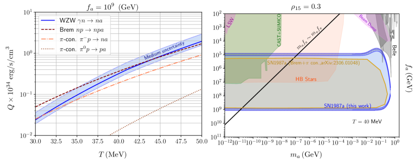
Figure 2: Left panel: Comparison of the emissivity rates from axion bremsstrahlung and pion conversion from [46, 64] with WZW photo-production (blue line) and medium uncertainties (blue shaded region). Right panel: The blue region shows the constraints drawn from WZW photo-production of axions and the hatched region represents the medium uncertainty. We recast the previous bounds [65] on axion parameter space from bremsstrahlung and pion conversion in yellow. Bounds on effective axion-photon coupling $g_{a\gamma\gamma}$ [66, 67], from HB stars [68, 69], CAST [70], Sumico [67] and light shining through wall [71] experiment is converted using Eqs. (6) and (5) onto the $m_{a}-f_{a}$ plane by identifying $f_{a}=\left(2\alpha_{em}C_{A}/\pi\right)\Lambda$ (see [66], Fig. 28). Exclusion limits from beam dump experiments [14, 15, 16], rare decays of $K$ [23, 27] and $B$-mesons [28, 29, 30] are shown in magenta and grey respectively.

Cooling via Axions.– As depicted in Fig. 1, Eq. (6) and Eq. (7) provide an efficient production channel of axions in a nucleon rich environment. The coupling $f_{a}$, dictates whether the axions can come out of the stellar object or get trapped inside it. In the former case, axions can carry a part of the internal energy of the core with them, resulting in the cooling of the star. To estimate, we compute the emissivity $Q$, defined as the emitted energy per unit volume and per unit time. We take into account both neutron degenerate (D) as well as non-degenerate (ND) scenarios, mimicking the situation inside an NS and SN respectively. The emissivity for axion photo-production $\gamma N\to Na$ is given by

$$Q^{\rm WZW}_{N\gamma\to Na}\equiv\int\frac{d^{3}\vec{p}_{\gamma}f_{\gamma}\left(p_{\gamma}\right)}{(2\pi)^{3}2E_{\gamma}}\int\frac{d^{3}\vec{p}_{N_{1}}}{(2\pi)^{3}2E_{N_{1}}}\frac{d^{3}\vec{p}_{N_{2}}}{(2\pi)^{3}2E_{N_{2}}}$$

$$g_{\gamma}\,g_{N}\int\frac{d^{3}\vec{p}_{a}}{(2\pi)^{3}2E_{a}}E_{a}\langle|\mathcal{M}|^{2}\,\rangle f_{N}(E_{N_{1}})\,(1-f_{N}(E_{N_{2}}))$$

$$\quad\times\,(2\pi)^{4}\delta(E_{N_{1}}-E_{N_{2}}-Q_{0})\,\delta^{3}(\vec{p}_{N_{1}}-\vec{p}_{N_{2}}-\vec{q})\,.$$ (8)

where $g_{\gamma(N)}=2$ are the dof. of the photon (neutron), $f_{N}$ is the neutron distribution function, $E_{i}$ and $\vec{p}_{i}$ are the energies and three-momenta of the $i^{\rm th}$ species and $Q_{0}\equiv E_{a}-E_{\gamma},\;\vec{q}\equiv\vec{p}_{a}-\vec{p}_{\gamma}$. The kinematics of the process is similar to a fixed target experiment where the initial neutron is assumed to be at rest. Due to the momentum transfer, the final neutron receives a kick and we consider them to be nearly non-relativistic, expanding in the energies $E_{N_{i}}\approx m_{N}+\mathcal{O}(\vec{p}^{2}_{N_{i}}/2m_{N})$. The spin averaged amplitude squared $\langle|\mathcal{M}|^{2}\rangle$ is

$$\langle|\mathcal{M}^{\rm WZW}_{\gamma N\to Na}|^{2}\rangle \approx\frac{8\kappa^{2}m_{N}^{2}}{f_{a}^{2}}\;\frac{g_{\omega}^{2}}{m_{\omega}^{4}}\;E_{\gamma}^{2}|\vec{p}_{a}|^{2}\;\sin^{2}\theta\;.$$ (9)

Here, $\theta$ is the angle between the axion and photon three momenta. The kinematics of the process dictates $E_{a}\sim E_{\gamma}$ when $m_{\gamma}\ll T$. This is a reasonable approximation as in the core of SN, the photons acquire a mass of the order of $m_{\gamma}\sim\mathcal{O}(10)\;\text{MeV}\times(Y_{e}\rho_{14})^{1/3}$, where $Y_{e}$ is the electron fraction. Since $T/m_{\gamma}\sim(3-4)$, we therefore do not expect the mass of the photon to play a significant role.

Non-degenerate scenario.– For ND neutrons, the absence of Pauli blocking helps us to further simplify Eq. (Anomaly Induced Supernovae Cooling: New Contribution from Axions) as $1-f_{N}(p_{N})\approx 1$. Using the thermal distribution for photons [72] and integrating the axion energy from $(m_{a},\infty)$, we find

$$Q_{N\gamma\to Na}^{\rm WZW,ND}\approx \;g_{\gamma}g_{\omega}^{2}\;\frac{\kappa^{2}n_{b}}{2\pi^{3}}\;\frac{T^{2}}{f_{a}^{2}}\;\frac{m_{a}^{4}}{m_{\omega}^{4}}\;\left[4m_{a}T\;K_{3}\left(\frac{m_{a}}{T}\right)\right.$$

$$\left.+(m_{a}^{2}+35T^{2})\;K_{4}\left(\frac{m_{a}}{T}\right)\right]\;,$$ (10)

where $K_{3,4}$ are the Bessel function of type three and four respectively. Further, the number density reads as

$$n_{b}=4.5\times 10^{-3}\rho_{15}\;\text{GeV}^{3},\quad\rho_{15}\equiv\rho/10^{15}\text{g cm}^{-3}\,.$$ (11)

In the limit of $m_{a}\to 0$, the expression in Eq.(10) further simplifies to

$$\frac{Q_{\gamma N\to Na}^{\rm WZW,ND}}{10^{34}\;\text{erg/s/cm}^{3}}\approx \;5.6\;C_{A}^{2}\;g_{40}^{4}\;T_{40}^{8}\,\rho_{15}\left(\frac{10^{9}\;\text{GeV}}{f_{a}}\right)^{2}\;,$$ (12)

here we define $T_{40}$ as $(T/40~{}\text{MeV})$ and $g_{40}\equiv(g_{\omega}/40)$. The temperature dependence in Eq. (12) can be understood as the phase space scales as $T^{3}$, the cross-section and emitted energy as $T^{4}$ and $T$ respectively. However, the cooling argument in Eq. (2) applies only when the axions can free-stream through the SN core and do not get trapped[38]. The mean free path can be deduced from $\ell=\left(n_{b}\sigma\right)^{-1}$ and can be approximated by

$$\frac{L_{a}}{10\;\text{Km}}\approx\frac{\rho_{15}^{-1}}{C_{A}^{2}}\;\frac{1}{g_{40}^{2}}\left(\frac{f_{a}}{10^{9}~{}\text{GeV}}\right)^{2}\left(\frac{1~{}\text{GeV}}{E_{a}}\right)^{4}\;.$$ (13)

This translates to an upper bound on the energy of the escaping axion. Therefore, Eq. (10) was an estimate based only on free-streaming axions. We impose this upper cut-off on the axion energy while deriving the final limits on the axion parameter space, shown in the right panel Fig. 2.

Degenerate scenario.–The derivation of the cooling rate is more involved when neutrons are degenerate inside a medium. We closely follow the derivation of Ref. [59] (see also Sup. mat.) to write the emissivity in terms of the momentum transfer and obtain,

$$\frac{Q_{\gamma N\to Na}^{\rm WZW,D}}{10^{34}\text{erg/s/cm}^{3}}\approx 1.7\;C_{A}^{2}\;g_{40}^{4}T_{40}^{9}\bigg{(}\frac{10^{9}~{}\text{GeV}}{f_{a}}\bigg{)}^{2}\,.$$ (14)

The final emissivity is given by the minimum of the degenerate and the non-degenerate expressions: $Q=\text{Min}[Q_{\rm D},Q_{\rm ND}]$. At the saturation density $\rho\sim\rho_{0}\approx 0.3\times 10^{15}\text{g cm}^{-3}$, we obtain that the rate is

$${}Q^{N\gamma\to Na}=\begin{cases}Q^{N\gamma\to Na}_{\rm D}\qquad T\lesssim 40\text{MeV}\\ Q^{N\gamma\to Na}_{\rm ND}\qquad T\gtrsim 40\text{MeV}\end{cases}$$ (15)

and we conclude that for the SN, it suffices to use the ND limit. On the left panel of Fig. 2, we show the emissivity of the photo-production and compare it with pion conversion and bremsstrahlung.

At this point, it is worth mentioning that the high densities in the SN cores lead to the modification of the masses and the couplings. The Brown-Rho scaling dictates that the variation of the mass of the vector mesons follows the neutron mass[73]:

$${}\frac{f_{\pi}^{\star}}{f_{\pi}}\approx\frac{m^{\star}_{\omega}}{m_{\omega}}\approx\frac{m^{\star}_{N}}{m_{N}}\Rightarrow\frac{g_{\omega}^{\star}}{g_{\omega}}\approx\frac{g_{\pi}^{\star}}{g_{\pi}}\approx\frac{g_{A}^{\star}}{g_{A}}\,.$$ (16)

where the $\star$ indicates that the quantity is evaluated in the dense environment of the NS [41, 72, 74]. The $m_{N}$ dependence is obtained from [75, 74]. For the $g_{A}$ dependence, we use two different scaling laws: thick line from[76, 41] and dashed line from[77, 78], $g_{A}^{\star}/g_{A}\approx 1/(1+(1/3)(m^{\star}_{N}/m_{N})(\rho/\rho_{0})^{1/3})$. In the case of the axion bremsstrahlung, such effects were lead to only moderate uncertainties in the coupling[79, 41]. For $\rho/\rho_{0}\in[0.5,1]$, the uncertainties in the WZW photo production amounts to

$${}\frac{Q^{\star}_{N\gamma\to Na}}{Q_{N\gamma\to Na}}\approx\frac{m_{\omega}^{4}}{g_{\omega}^{4}}\frac{g_{\omega\star}^{4}}{m_{\omega\star}^{4}}\in[0.8,1.5]\;.$$ (17)

Implications.– We summarize our results in fig. 2 where we show WZW photo-production with $T=40$ MeV can exclude regions with $f_{a}\lesssim 10^{9}$ GeV for $m_{a}\lesssim 100$ MeV. The previous constraints, deduced from simulations in[65], reaches $f_{a}\lesssim 0.77\times 10^{9}$ GeV for $m_{a}\lesssim 50$ MeV. We see that the combination of the two rates would bring a factor $\mathcal{O}(2-3)$ with respect to the previous bound from bremsstrahlung and pion conversion only. We note in passing that axion photo-production can also be induced via the electric dipole portal [49]. However, the constraints are far subleading, $f_{a}/\text{GeV}\gtrsim 6\times 10^{5}$ compared to WZW process. As a consequence, we also neglect the possible cross terms between the WZW and the electric dipole that could arise.

It is also important to mention that the landscape of QCD axion models is quite broad. Without going into the details of such different scenarios, we consider a minimal situation given by Eq. (1), similar to the KSVZ [80, 81] framework. However, we find that similar conclusions hold in other types of axion models such as DFSZ [82, 83] (see Sup. Mat.). This demonstrates the robustness of the WZW term as far as cooling of SN is concerned.

The emissivity is related to the number density of particles emitted via

$${}Q_{\rm a}=\int dE_{a}E_{a}\frac{d^{2}n_{a}}{dE_{a}dt}\,,$$ (18)

where the spectrum is defined as the number of axions emitted per interval of energy and time. Comparing with Eq. (Anomaly Induced Supernovae Cooling: New Contribution from Axions), it is straightforward to obtain the spectrum in the ND limit and for $m_{a}\ll T$. Furthermore, the total emitted flux is well approximated by integrating the spectrum over the radius of the star in the optically thin limit. Taking $R_{\rm PNS}\approx 10$ Km, we obtain

$$\frac{d^{2}N_{a}}{dE_{a}dt}\approx C_{f} \rho_{15}\bigg{(}\frac{C_{A}10^{9}}{f_{a}/\text{GeV}}\bigg{)}^{2}g^{4}_{40}\bigg{(}\frac{E_{a}}{\text{MeV}}\bigg{)}^{6}e^{-E_{a}/T}\;,$$

$$C_{f} =4.6\times 10^{42}\;\text{MeV}^{-1}\text{s}^{-1}\,.$$ (19)

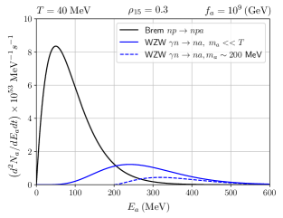
As shown in Fig. 3 by the blue curve, the total flux from the WZW photo-production is distinctively different from axion bremsstrahlung, with a comparatively harder spectrum.

Figure 3: Spectrum of axions due to WZW photo-production (blue) and bremsstrahlung [74] (black).

Axion detection prospects.– Finally, we discuss the prospect of detecting such axions in Water Cerenkov experiments [39] such as Hyper-Kamiokande with fiducial mass 374 ktons [84]. Usually, axions emitted during future galactic SN can interact with the detector via the channels $ap\to p\gamma$ and $ap^{+}\to n\pi^{+}$ [49]. Around the peak of the WZW axion spectrum, i.e., $E_{a}\sim 200-300$ MeV, the cross section for $ap^{+}\to n\pi^{+}$ is dominated by the $\Delta(1.23~{}\text{GeV})$ resonance and roughly translates to $\sigma_{ap^{+}\to N\pi^{+}}\approx 10^{-25}C_{A}^{2}(f_{\pi}/f_{a})^{2}$ cm^-2 [85]. Assuming $N_{t}$ target particles, the spectrum of produced particles ($\gamma$ or $\pi$) from axions is

$$\frac{d^{2}N_{p}}{dtdE_{p}}=\frac{N^{p}_{t}}{4\pi(d/\text{Kpc})^{2}}\times\frac{d^{2}N_{a}}{dtdE_{a}}\left(\frac{\sigma_{2\to 2}}{\text{cm}^{2}}\right),$$ (20)

$$\;N^{p}_{t}\approx 2\times 10^{9}N_{a}\bigg{(}\frac{M_{\rm detector}}{\text{kton}}\bigg{)}\bigg{(}\frac{\text{g}/\text{mol}}{m_{H_{2}O}}\bigg{)}\,.$$

where $N_{a}$ is the Avogadro number, $m_{H_{2}O}=18\text{g}/\text{mol}$ the molecular mass of water, and $d$ is the distance to the SN.

For small momentum transfer, the energy of the final state particle is roughly equal to the energy of the incoming axion, i.e., $E_{p}\simeq E_{a}$. For constant cross-sections with $100-500$ MeV axions, the produced particle will inherit the spectrum of the emitted axions. The number of pions produced during such interaction can be obtained by integrating Eq.(20) and we find

$${}\frac{dN_{\pi}}{dt}\approx 6\;\rho_{15}\;C_{A}^{4}\;\bigg{(}\frac{10^{9}}{f_{a}/\text{GeV}}\bigg{)}^{4}g^{4}_{40}\,T_{40}^{7}\bigg{(}\frac{\text{Kpc}}{d}\bigg{)}^{2}$$

$$\times\bigg{(}\frac{M_{\rm detector}}{\text{kton}}\bigg{)}\bigg{(}\frac{\text{g}/\text{mol}}{m_{H_{2}O}}\bigg{)}\,s^{-1}\,.$$ (21)

A SN at a distance of 1 Kpc with axions having $f_{a}=10^{9}$ GeV, would thus roughly produce $\sim 5$ pions in the Hyper-Kamiokande, on a timescale of 10 seconds. On the other hand, the number of photons produced via $ap\rightarrow p\gamma$ is always negligible because of a smaller cross-section.

Summary & outlook.– In summary, we point out a new channel for axion photo-production, i.e., $\gamma N\to Na$, mediated by the WZW term $\epsilon^{\mu\nu\alpha\beta}F_{\mu\nu}\;\partial_{\alpha}a\;\omega_{\beta}$. We find that for temperatures $T\gtrsim 30$ MeV, the WZW photo-production emissivity can compete and even dominate over the usual axion bremsstrahlung process $NN\to NNa$, as depicted in Fig. 2 This is because the three-body phase space suppression of the bremsstrahlung competes with the loop suppression arising from the anomaly-induced WZW term. As a result, the WZW process can increase the SN cooling rate by a factor of 2-3 and should be considered in the SN simulations [86]. Moreover, the spectrum of such axions is distinctively different compared to the prototypical SN cooling processes. As a result, WZW axions emitted from a close-by SN can leave a smoking-gun signature in the near future Water Cherenkov experiments, producing $\mathcal{O}(10)$ pions in the final state. Photo-production of axions can also be probed at GlueX[87], where the photon beam of $\sim 10$ GeV hits a fixed target and produces a plethora of mesons. As far as degenerate neutron stars are concerned, we find that the cooling rate scales as $T^{9}$ and is subdominant compared to $NN\to NNa$ for temperatures $T\lesssim 30$ MeV.

At this point, it is pertinent to ask whether there exist SM WZW interactions such as $\epsilon^{\mu\nu\rho\sigma}F_{\mu\nu}\omega_{\rho}Z_{\sigma}$ that can lead to SN cooling. Such interactions induce the process $\gamma N\to N\nu\bar{\nu}$ resulting in the emission of a pair of neutrinos from the decay of an off-shell $Z$ boson. It was found in [59], that the emissivity from such interactions can play a significant role for NS with degenerate stellar cores when $T>10-20$ MeV. For SN, WZW induced SM photo-production of neutrinos can dominate compared to other processes around $T\sim 40$ MeV. However, further investigation is required as the neutrinos at such temperatures might get trapped [88]. Finally, assuming purely non-relativistic neutrons and a large magnetic field, the axion WZW term reduces to a mixing between $a-\omega$ field or can also contribute to axion-photon oscillation in the presence of a varying neutron density. Naturally, the phenomenological implications are rich, interesting and need to be explored further.

SC thanks the Science and Engineering Research Board, Govt. of India (SRG/2023/001162) for financial support. MV is supported by the “Excellence of Science - EOS” - be.h project n.30820817, and by the Strategic Research Program High-Energy Physics of the Vrije Universiteit Brussel. AG is supported by the “Generalitat Valenciana” and CSIC through the GenT Excellence Program (CIDEIG/2022/22). MV thanks IFIC (Valencia) and CSIC for their hospitality during the completion of this project and Alberto Mariotti for comments on the draft.

I Wess-Zumino-Witten Interactions

The dynamics and interactions of Goldstones bosons associated with the spontaneous breaking of chiral symmetry is aptly described by the Chiral Lagrangian ($\chi$PT). At the leading order, the Lagrangian consists of terms

$$\mathcal{L}=\frac{f_{\pi}^{2}}{4}\text{Tr}\left(D_{\mu}U^{\dagger}D^{\mu}U+U^{\dagger}\chi+\chi^{\dagger}U\right)\;,$$ (22)

where $D_{\mu}U=\partial_{\mu}U-ir_{\mu}U+iU\ell_{\mu}$. $r_{\mu}$ and $\ell_{\mu}$ describe left and right-handed currents which can be used to construct the vector and axial vector currents. Moreover, $\chi=2B_{0}\mathcal{M}$, where $\chi$ is the isospin symmetry breaking spurion with $\mathcal{M}$ denoting the quark mass matrix. Constants $B_{0}$ and $f_{\pi}$ are fixed by experiments. However, Eq. (22) possesses more symmetries such as spurious parity and charge conjugation compared to its underlying UV theory, i.e., QCD. As a result, $\chi$PT in Eq. 22 fails to describe processes such as $K^{+}K^{-}\to\pi^{+}\pi^{-}\pi^{0}$ and $\pi^{0}\to\gamma\gamma$, which are otherwise allowed in QCD. Such interactions can be restored in the Chiral Lagrangian by the Wess-Zumino-Witten term. In the geometric representation of the WZW form, one considers a 5-dimensional action, whose boundary is identified with 4-dimensional space in the form

$$S_{WZW}(U)=\kappa\int_{D}d^{5}y\;\omega\;,\;\text{where}\;\;\omega=-\frac{i}{240\pi^{2}}\epsilon^{\mu\nu\rho\sigma\tau}\;\text{Tr}\left[\;\mathcal{U}_{\mu}\;\mathcal{U}_{\nu}\;\mathcal{U}_{\rho}\;\mathcal{U}_{\sigma}\;\mathcal{U}_{\tau}\right]\;.$$ (23)

Here, we define $\mathcal{U}_{\mu}=U^{\dagger}\partial_{\mu}U$ and $\mathcal{U}\approx\text{Exp}\left(2i\pi^{a}T^{a}/f_{\pi}\right)$ with $f_{\pi}=93$ MeV. Under chiral symmetry, $U$ transforms as $U\to RUL^{\dagger}$ with $R$ and $L$ describing the $SU(2)_{R}$ and $SU(2)_{L}$ transformation matrices. Note that Eq. (23) correctly describes the process $K^{+}K^{-}\to\pi^{+}\pi^{-}\pi^{0}$. To generate $\pi^{0}\to\gamma\gamma$ or similar processes, one has to gauge $S_{WZW}$. However, any gauging has to be done in the 4-dimension. In principle, any arbitrary subgroup of the WZW action can be gauged and the resultant terms are

$$S_{WZW}\left(U,A_{L},A_{R}\right)=S_{WZW}\left(U\right)+\frac{N_{c}}{48\pi^{2}}\int d^{4}x\;\epsilon^{\mu\nu\rho\sigma}\;Z_{\mu\nu\rho\sigma}\;,$$ (24)

where the full expression of $Z_{\mu\nu\rho\sigma}$ has been nicely tabulated in Ref. [51]. However, for our work, we only track the pion fields and therefore the relevant terms are

$$Z_{\mu\nu\rho\sigma}(U,A_{L},A_{R})\supset i\; \text{Tr}\left[\left\{\left(\partial_{\mu}A_{\nu_{L}}\right)A_{\rho_{L}}+A_{\mu_{L}}(\partial_{\nu}A_{\rho_{L}})\right\}\partial_{\sigma}U\;U^{-1}+\left\{\left(\partial_{\mu}A_{\nu_{R}}\right)A_{\rho_{R}}+A_{\mu_{R}}(\partial_{\nu}A_{\rho_{R}})\right\}U^{-1}\partial_{\sigma}U\right]$$

$$+ i\;\text{Tr}\left[\left\{(\partial_{\mu}A_{\nu_{R}})\;U^{-1}A_{\rho_{L}}\partial_{\sigma}U+A_{\mu_{L}}U^{-1}(\partial_{\nu}A_{\rho_{R}})\;\partial_{\sigma}U\right\}\right]\;.$$ (25)

Expanding in pion fields, $\partial_{\mu}U$ can be written as

$$\partial_{\mu}U=i\frac{\partial_{\mu}\pi_{0}}{f_{\pi}}\begin{pmatrix}1&0\\ 0&-1\end{pmatrix}+...\,.$$ (26)

This choice results in a canonically normalized kinetic term from $\pi_{0}$. Moreover, in the SM, the gauge fields are expressed as

$$A_{L}=g_{2}W^{a}\frac{\tau^{a}}{2}+g_{1}W^{0}\;\begin{pmatrix}\frac{1}{6}&0\\ 0&\frac{1}{6}\end{pmatrix}\;,\;\;\;A_{R}=g_{1}W^{0}\;\begin{pmatrix}\frac{2}{3}&0\\ 0&-\frac{1}{3}\end{pmatrix}\;.$$ (27)

The physical gauge fields $A$ and $Z$ are introduced after electroweak symmetry breaking and they are related with $W^{0}$ and $W^{3}$ fields via the weak rotation angle $\theta_{w}$ as

$$W^{0}=-s_{W}Z+c_{W}A,\qquad W^{3}=c_{W}Z+s_{W}A\,.$$ (28)

Using $g_{1}c_{W}=g_{2}s_{W}=e$, Eq. (27) becomes

$$A_{L}=g_{2}s_{W}\frac{A}{2}\begin{pmatrix}1&0\\ 0&-1\end{pmatrix}+g_{1}c_{W}A\begin{pmatrix}\frac{1}{6}&0\\ 0&\frac{1}{6}\end{pmatrix}=eA\begin{pmatrix}\frac{2}{3}&0\\ 0&-\frac{1}{3}\end{pmatrix}=A_{R}\,,$$ (29)

To introduce the vector mesons fields, we use the background field method presented in Ref. [56] where $\widetilde{A}_{L,R}=A_{L,R}+B_{L,R}$ (the charge as been included inside the definition of the field), including both the fundamental and background gauge fields. As a result, we make the following replacement $A_{L,R}\to\widetilde{A}_{L,R}$ in Eq. (25). The background field $\omega$ is then identified as

$$B_{V}=\frac{2g_{\omega}}{3}\;\omega\begin{pmatrix}1&0\\ 0&1\end{pmatrix}\,,\qquad B_{A}=0\,,\;\;\;\Rightarrow B_{L}=B_{R}=\frac{B_{V}}{2}=\frac{g_{\omega}}{3}\;\omega\begin{pmatrix}1&0\\ 0&1\end{pmatrix}\,.$$ (30)

Using the definition of $A_{L,R}$ and $B_{L,R}$ as well as $N_{c}=3$, fixed by matching with QCD, we find from Eq. (25)

$$\mathcal{L}_{\rm WZW}\supset\frac{N_{c}}{24\pi^{2}}eg_{\omega}\frac{\partial_{\rho}\pi_{0}}{f_{\pi}}\epsilon^{\mu\nu\rho\sigma}F_{\mu\nu}\;\omega_{\sigma}+\frac{N_{c}}{96\pi^{2}}e^{2}\;\epsilon^{\mu\nu\rho\sigma}\;\frac{\pi_{0}}{f_{\pi}}F_{\mu\nu}F_{\rho\sigma}\;.$$ (31)

The coefficient $N_{c}=3$ is fixed by matching with QCD.

II Computation of the emissivities for the axion

In this section, we present the computation of the emissivities of the WZW photo-production reaction $\gamma N\to Na$ for the non-degenerate case and then for the degenerate case.

II.1 Emissivity in the non-degenerate case

We study the $2\to 2$ interaction $\gamma N\to Na$ in the non-degenerate limit. In the centre of mass frame of the collision, $E_{CM}=E_{N_{1}}+E_{\gamma}=E_{N_{2}}+E_{a}$. The matrix element takes the form

$$\langle|\mathcal{M}|^{2}\rangle =8\frac{\kappa^{2}m_{N}^{2}g_{\omega}^{2}}{f_{a}^{2}m_{\omega}^{4}}\bigg{(}E_{\gamma}^{2}|\vec{p}_{a}|^{2}\sin^{2}\theta\bigg{)}+\mathcal{O}(p_{F}^{2}/m_{N}^{2}),\qquad\kappa\equiv C_{A}\frac{eN_{c}}{24\pi^{2}}g_{\omega}\,,$$ (32)

where we neglect $m_{\gamma}$ compared to the energy scale. $\theta$ is the angle between the incoming neutron and the outgoing axion, $p_{F}$ is the Fermi momentum of neutrons. Also, $E_{i}$ and $\vec{p_{i}}$ are the energy and three-momenta of the $i^{\rm th}$ species. In the CM frame

$$E_{\rm CM}\equiv E_{N_{1}}+E_{\gamma}=E_{N_{2}}+E_{a}\;,\qquad E_{\gamma}\approx E_{a}\;,\qquad E_{a}^{2}=p_{a}^{2}+M_{a}^{2}\,.$$ (33)

The cross-section for the $N\gamma\to Na$ process is given by

$$\frac{d\sigma_{N\gamma\to Na}}{d\Omega} =\frac{|\vec{p}_{a}|}{|\vec{p}_{\gamma}|}\frac{\langle|\mathcal{M}|^{2}\rangle}{64\pi^{2}E_{CM}^{2}}\theta\left(E_{cm}-m_{N}-m_{a}\right)\;,$$

$$=\frac{\sqrt{E_{a}^{2}-m_{a}^{2}}}{E_{\gamma}}\frac{\langle|\mathcal{M}|^{2}\rangle}{64\pi^{2}E_{CM}^{2}}\theta(E_{CM}-m_{N}-m_{a})\;,$$

$$\approx\frac{\sqrt{E_{a}^{2}-m_{a}^{2}}}{E_{\gamma}}\frac{\langle|\mathcal{M}|^{2}\rangle}{64\pi^{2}m_{N}^{2}}\theta(E_{CM}-m_{N}-m_{a})\,.$$ (34)

The emissivity rate in the non-degenerate limit is expressed as

$$Q^{\gamma N\to Na}_{\rm ND} \approx\int\frac{g_{\gamma}d^{3}\vec{p}_{\gamma}}{(2\pi)^{3}}f_{\gamma}(p_{\gamma})\int\frac{g_{N}d^{3}\vec{p}_{N}}{(2\pi)^{3}}f_{N}\int\frac{\langle|\mathcal{M}|^{2}\rangle}{4E_{N_{1}}E_{\gamma}}(2\pi)^{4}\delta^{4}\left(\sum_{i}p_{i}\right)\frac{d^{3}\vec{p_{2}}d^{3}\vec{p_{a}}}{(2\pi)^{6}4E_{a}E_{N_{2}}}E_{a}\,.$$ (35)

which can be further simplified with

$$Q^{\gamma N\to Na}_{\rm ND} \approx\int\frac{g_{\gamma}d^{3}\vec{p_{\gamma}}}{(2\pi)^{3}}f_{\gamma}(p_{\gamma})\int\frac{g_{N}d^{3}\vec{p}_{N}}{(2\pi)^{3}}f_{N}\sigma(E_{\gamma})E_{a}\;,\qquad\sigma(E_{\gamma})\approx\frac{1}{3\pi}\frac{\kappa^{2}g_{\omega}^{2}}{f_{a}^{2}m_{\omega}^{4}}\sqrt{1-\frac{M_{a}^{2}}{E_{\gamma}^{2}}}E_{\gamma}^{2}(E_{\gamma}^{2}-M_{a}^{2})\,,$$ (36)

where $\sigma(E_{\gamma})$ is the integrated cross section. The nucleon density is given by

$$n_{B}\equiv\int\frac{d^{3}p_{N}}{(2\pi)^{3}}g_{N}f_{N},\qquad n_{B}=4.5\times 10^{6}\rho_{15}\text{ MeV}^{3}\,.\\$$ (37)

Plugging Eq.(37) in the emissivity Eq.(36), we obtain

$$Q^{N\gamma\to Na}_{\rm ND} \approx\frac{g_{\gamma}n_{B}}{3\pi}\frac{\kappa^{2}g_{\omega}^{2}}{f_{a}^{2}m_{\omega}^{4}}\int^{\infty}_{m_{a}}\frac{dE_{\gamma}}{2\pi^{2}}f_{\gamma}(p_{\gamma})E_{\gamma}^{5}(E_{\gamma}^{2}-m_{a}^{2})\sqrt{1-\frac{m_{a}^{2}}{E_{\gamma}^{2}}}\,.$$ (38)

The two limiting conditions are:

1. $m_{a}/T\to 0$: In the limit $m_{a}/T\to 0$, we can approximate $\sqrt{1-\frac{m_{a}^{2}}{E_{\gamma}^{2}}}\to 1$. This results in

   $$Q^{N\gamma\to Na}_{\rm ND}\approx\frac{g_{\gamma}n_{B}}{3\pi^{3}}\frac{4\pi^{8}}{15}\frac{\kappa^{2}g_{\omega}^{2}}{f_{a}^{2}m_{\omega}^{4}}T^{8}\approx 27g_{\gamma}n_{B}\frac{\kappa^{2}}{f_{a}^{2}}T^{8}\;.$$ (39)

   Using the values and the normalization of the parameters explained in the main text along with $g_{\gamma}=2$, we get

   $$Q^{N\gamma\to Na}_{\rm ND}\approx 12\times C^{2}_{A}\bigg{(}\frac{g_{\omega}}{10}\bigg{)}^{4}\frac{n_{B}}{m_{\omega}^{4}f_{a}^{2}}T^{8}\;\Rightarrow\frac{Q^{N\gamma\to Na}_{\rm ND}}{5.6\times 10^{34}\text{erg/s/ cm}^{3}}\approx\bigg{(}\frac{C_{A}m_{N}10^{9}}{f_{a}}\bigg{)}^{2}\times g_{40}^{4}\rho_{15}T_{40}^{8}\,.$$ (40)

2. $m_{a}/T\gtrsim 1$: In the opposite limit $m_{a}/T\gtrsim 1$, the mass of the axion cannot be neglected anymore and the expression becomes

   $$\frac{Q^{N\gamma\to Na}_{\rm ND}}{1.1\times 10^{31}\text{erg/s/ cm}^{3}}\approx\bigg{(}\frac{C_{A}m_{N}10^{9}}{f_{a}}\bigg{)}^{2}g_{40}^{4}\times\rho_{15}G(m_{a},T_{40})\,,$$ (41)

   where we defined the $G$ function in terms of the Bessel functions as

   $$G(m_{a},T)\equiv 3m_{a}^{4}T^{2}\bigg{(}4m_{a}TK_{3}\bigg{(}\frac{m_{a}}{T}\bigg{)}+(m_{a}^{2}+35T^{2})K_{4}\bigg{(}\frac{m_{a}}{T}\bigg{)}\bigg{)}\,.$$ (42)

II.2 Emissivity in the degenerate case

We now evaluate the emissivity in the presence of strongly degenerate neutrons. The full expression is provided in a convenient form as

$$Q^{N\gamma\to Na}_{\rm axion}=2\frac{\kappa^{2}}{f_{a}^{2}}\int\dfrac{d^{3}\vec{p}_{\gamma}}{(2\pi)^{3}}g_{\gamma}\dfrac{f_{\gamma}}{2E_{\gamma}}\int\dfrac{d^{3}\vec{p}_{a}}{(2\pi)^{3}2E_{a}}\times\bigg{[}2E_{\gamma}E_{a}(p_{\gamma}\cdot p_{a})-(p_{\gamma}\cdot p_{a})^{2}\bigg{]}\,S(q^{\mu})E_{a}\,.$$ (43)

where we define $Q_{0}\equiv E_{2}-E_{1}=E_{\gamma}-E_{a}\;,\qquad\vec{q}=\vec{p}_{\gamma}-\vec{p}_{a}$. The response function is defined as

$$S(q^{\mu})\equiv g_{N_{1}}\int\dfrac{d^{3}\vec{p}_{N_{1}}d^{3}\vec{p}_{N_{2}}m_{N}^{2}}{(2\pi)^{6}\,E_{N_{1}}\,E_{N_{2}}}f_{N}(E_{N_{1}})(1-f_{N}(E_{N_{2}}))\times(2\pi)^{4}\times$$

$$\delta(E_{N1}+Q_{0}-E_{N_{2}})\delta^{3}(\vec{p}_{N_{1}}-\vec{p}_{N_{2}}+\vec{q})\,\Theta(E_{N_{1}}-m_{N})\,\Theta(E_{N_{2}}-m_{N})\;,$$ (44)

and can be computed while identifying $z=Q_{0}/T$ and $|\vec{q}|\equiv q$. We obtain the final form of the response function

$$S(Q_{0},q)=\dfrac{M_{N}^{2}\,Q_{0}}{\pi q}\dfrac{1}{1-e^{-z}}\Theta(\mu-E_{-}).$$ (45)

$$E^{-}=\sqrt{\bigg{(}m_{N}+\frac{Q_{0}}{2}\bigg{)}^{2}+\bigg{(}\frac{\sqrt{q^{2}-Q_{0}^{2}}}{2}-\frac{m_{N}Q_{0}}{\sqrt{q^{2}-Q_{0}^{2}}}\bigg{)}^{2}}-\left(m_{N}+\frac{Q_{0}}{2}\right)\,.$$ (46)

which can be simplified further

$$E^{-}\approx\sqrt{m_{N}^{2}+\bigg{(}\frac{m_{N}Q_{0}}{\sqrt{q^{2}-Q_{0}^{2}}}\bigg{)}^{2}}-m_{N}\,.$$ (47)

To perform the integral over $p_{a}$, we make the following change of variables

$$qdq=E_{a}E_{\gamma}d\cos\theta,\qquad dQ_{0}=dE_{a}\qquad\xrightarrow{}\quad\int\frac{d^{3}p_{a}}{(2\pi)^{3}2E_{a}}=\int\frac{dQ_{0}dqq}{(2\pi)^{2}2}\frac{1}{E_{\gamma}}\,,$$ (48)

and the integral becomes

$$Q^{N\gamma\to Na}_{\rm D}=\frac{g_{\gamma}\kappa^{2}}{f_{a}^{2}}\int\dfrac{d^{3}p_{\gamma}}{(2\pi)^{3}}\dfrac{f_{\gamma}}{E_{\gamma}}\int\frac{dQ_{0}\,dq}{(2\pi)^{2}2E_{\gamma}}\dfrac{M_{N}^{2}\,Q_{0}}{\pi}\times\bigg{[}2E_{\gamma}E_{a}(p_{\gamma}\cdot p_{a})-(p_{\gamma}\cdot p_{a})^{2}\bigg{]}\dfrac{E_{\gamma}-Q_{0}}{1-e^{-Q_{0}/T}}\Theta(\mu-E_{-})\,.$$ (49)

The expression between the parenthesis in Eq.(49) can be rewritten

$$\bigg{[}2E_{\gamma}E_{a}(p_{\gamma}\cdot p_{a})-(p_{\gamma}\cdot p_{a})^{2}\bigg{]}=\bigg{[}(E_{\gamma}E_{a})^{2}-(\vec{p}_{\gamma}\cdot\vec{p}_{a})^{2}\bigg{]}\approx\frac{(q^{2}-Q_{0}^{2})}{4}\bigg{(}-(q^{2}-Q_{0}^{2})+4E_{\gamma}(E_{\gamma}-Q_{0})\bigg{)}\,.$$ (50)

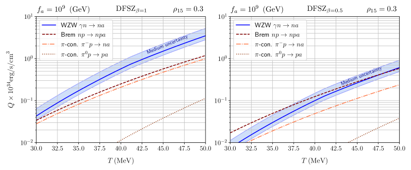
Figure 4: Comparison plots for the DFSZ model.

To perform the integral, we need to define the boundaries of integration. Kinematics impose the condition that $q$ variable varies from $q\in[Q_{0},2E_{\gamma}-Q_{0}]$. The Theta function in Eq.(49) combined with the expression for $E_{-}$ in Eq.(47) further impose the lower bound on the $q$ region of integration as $b|Q_{0}|$. In the end, we get

$$q\in\bigg{[}b|Q_{0}|,2E_{\gamma}-Q_{0}\bigg{]}\;,\qquad a\equiv(\mu_{N}/M_{N}+1)^{2}-1\,,\qquad b\equiv\sqrt{\frac{a+1}{a}}\,.$$ (51)

Taking the typical value $\mu_{N}=300$ MeV, we find $b\approx 1.56$. We will use those two values as a range of uncertainty for the degenerate density of the proto-NS. This induces that the $Q_{0}$ integral should be performed between

$$Q_{0}\in\bigg{[}-\frac{2}{b-1}E_{\gamma},\frac{2}{b+1}E_{\gamma}\bigg{]}\,.$$ (52)

We can further separate the parameter space into the region of

$$Q_{0}\in\bigg{[}-\frac{2}{b-1}E_{\gamma},0\bigg{]}\,,\qquad Q_{0}\in\bigg{[}0,\frac{2}{b+1}E_{\gamma}\bigg{]}\,.$$ (53)

The integral over $q$ can be trivially performed and by finishing the integration numerically, we obtain

$$\frac{Q_{N\gamma\to Na}^{\rm WZW,D}}{10^{34}\text{erg/s/cm}^{3}}\approx 1.7\;C_{A}^{2}\;g_{40}^{4}T_{40}^{9}\bigg{(}\frac{10^{9}~{}\text{GeV}}{f_{a}}\bigg{)}^{2}\,.$$ (54)

III Emissivity for different axion models

In generic axion and ALPs, models, the the ALP can have a myriad more couplings, namely directly to quarks and leptons, making the whole coupling structure quite model-dependent. To demonstrate the model dependence, we present the comparison between the pion conversion, the axion bremsstrahlung and the WZW photo-production in Fig.4 using the following parameterization[60]

$$C_{ap}=-0.47+0.29\cos^{2}\beta-0.13\sin^{2}\beta\,,\qquad C_{an}=-0.02+0.29\sin^{2}\beta-0.13\cos^{2}\beta\,.$$ (55)

We also find that only when $\beta\ll 1$, the WZW contribution subleading. When $\beta$ is larger, the enhancement of the emissivity is order $\mathcal{O}(2-3)$.