Are accelerated detectors sensitive to Planck scale changes?

Abstract

One of the foremost concern in the analysis of quantum gravity is whether the locations of classical horizons are stable under a full quantum analysis. In principle, any classical description, when interpolated to the microscopic level, can become prone to fluctuations. The curious question in that case is if there indeed are such fluctuations at the Planck scale, do they have any significance for physics taking place at scales much away from the Planck scale? In this work, we try to attempt the question of small scales and address whether there are definitive signatures of Planck scale shifts in the horizon structure. In a recent work Lochan and Padmanabhan (2021), it was suggested that in a nested sequence of Rindler causal wedges, the vacua of preceding Rindler frames appear thermally populated to a shifted Rindler frame. In fact, the Rindler frame $R_{n}$ attributes the vacuum states natural to the frames $R_{j}$ where $j<n$ (in addition to the inertial vacuum state) the same temperature $a_{n}/2\pi$ related to the acceleration of the frame $R_{n}$. Although the shift parameters, which give the separation between the causal domains, are at the heart of the inequivalence of these vacua, the results obtained through the Bogoliubov coefficients are insensitive to these parameters. The Bogoliubov analysis used, however, relies on the global notion of the quantum field theory and might be unable to see the local character of such horizon shifts. We investigate this system by means of the Unruh-DeWitt detector and see if this local probe of the quantum field theory is sensitive enough to the shift parameters to reveal any microscopic effects. For the case of infinite-time response, we recover the thermal spectrum, thus reaffirming that the infinite-time response probes the global properties of the field. On the other hand, the finite-time response turns out to be sensitive to the shift parameter in a peculiar way that any detector with energy gap $\Omega c/a\sim 1$ and is operational for time scale $Ta/c\sim 1$ has a measurably different response for a macroscopic and microscopic shift of the horizon, giving us direct probe to the tiniest separation between the causal domains of such Rindler wedges. Thus, this study provides an operational method to identify Planck scale effects which can be generalized to various other interesting gravitational settings. The implications of the results are also discussed.

I Introduction

The elusive quantum description of gravity has long kept us from gaining a better understanding not only of the physics near singularity but also about the effects of potential spacetime fluctuations, quantum gravity has to offer at the microscopic scales. In the discourse of quantum gravity, it is usually accepted that the spacetime described by a smooth metric, is only a macroscopic effective description arising out of some microscopic degrees of freedom. Perhaps at the microscopic level (which is traditionally believed to be the Planck scale), the degrees of freedom describing spacetime geometry would be quantum in nature. Their basic quantum character would therefore be most visible at the Planck scale itself Percival (1995). At such scales, the quantum uncertainty must prohibit a well defined geometric understanding and impart quantum fluctuations to the description.

Even much before the Planck scale, at the semiclassical level itself, since the dynamics of spacetime is essentially dictated by matter - which is fundamentally quantum in nature - it is also possible that the quantum matter imparts some uncertainty to the gravitational sector Hu and Verdaguer (2004). Thus, there may be induced fluctuations Salecker and Wigner (1958) from the matter side apart from any potential inherent uncertainty quantum gravity offers. Therefore, the macroscopic spacetime structure or the symmetries of metric that we hold dear might not hold in their truest form as we march towards probing length scales of smaller and smaller order. This may lead to distortion in the “classical metric” based analysis of modes which probe such scales, such as the dispersion relation of a free quantum field. It is worthwhile to ponder if there can be gedanken experiments that can capture and relay such effects to the macroscopic scales Husain and Louko (2016).

In that spirit, it is interesting to consider if light cones and various horizons are stable classical objects or if they also have some intrinsic quantum character, which macroscopic observations are oblivious about Ford (1995)? This particular thought becomes more pertinent in the context of black hole kinematics as well as its dynamics Ford and Svaiter (1997); Thompson and Ford (2008). If horizons do have some intrinsic quantum character, then black hole horizons may also be fuzzy and the standard analysis relying upon the availability of a definitive horizon (such as the Hawking radiation, the Unruh effect) may have some bearing Ford and Svaiter (1997).

Whatever be the origins of such randomness in the spacetime description, it is traditionally believed that by the time we arrive at the macroscopic levels, all such quantum characteristics are more or less lost, and the macroscopic physics becomes insensitive to the quantum fluctuations, the microscopic character is expected to harbor. Furthermore, since such quantum fluctuations are expected to take place on very short time scales, it is unclear how any detector operating over macroscopic time scales will not average out such fluctuations to lose their effects altogether. Moreover, even if higher moments (e.g., the variance) of such fluctuations can survive during such an averaging and a detector coupled to the higher moments can potentially capture such effects in principle, they are expected to be of the order of the Planck scale. Given the limited resolutions of experiments, one can anticipate such signatures to be of minuscule proportion to have any realistic consideration. Thus, the question of real relevance is if there are macroscopic detectors that can definitively capture Planck scale effects.

In a similar fashion, in the context of black hole dynamics, a question of interest is if the black hole horizons shift by Planck scale during their formation (or evaporation), do they leave any measurable imprint of their shift to the outside geometry at the macroscopic level? Such effects, if present, can have important implications for the information paradox as well Chakraborty and Lochan (2017). The trajectories which are to remain outside the black hole and make the judgment of the shift in the horizon are necessarily accelerated. Thus, it is more precisely a problem if detectors on accelerated trajectories can sense Planck scale shifts in a finite time duration of operation.

(a) Black hole horizon shifts with the addition of mass. The exterior observers have to adjust their accelerations to remain outside, lest they fall in

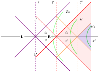
(b) Nested Rindler structure: Accelerated observers on Rindler trajectories find the vacuum state of all preceding Rindler observers thermally populated

Figure 1: Operational approach to introduce fuzziness in the Horizon structure. In the first case, it is achieved by the addition of an infinitesimal mass in the black hole and a microscopic shift in the causal domains in the second case.

In an attempt of answering these questions, as a convenient starting step, we pose the problem in the Rindler world in this work. Since in the Rindler space, there is truly no dynamical character to the horizon (at least classically), we investigate if two Rindler observers which have different horizons can distinguish each other through their detectors’ responses, particularly in the case when the horizons are microscopically separated (say by Planck scale shift). In Lochan and Padmanabhan (2021), it was demonstrated that the field theoretic particle content clearly distinguishes two Rindler frames apart if their domain of dependence are even marginally different. However, since in a strict field theoretic sense, all the characterization is done on a Cauchy surface, they are global in character (one needs to know the full spacetime a priori) and does not provide reliable estimates of local tests that try to estimate change in horizons.

In this work, we explore a local test to the study with the help of a finite time Unruh-DeWitt (UDW) detector response Unruh (1976). The UDW detector is an operational quantum device to probe quantum field configuration. It is a quantum mechanical system that is coupled to the quantum field, and when the field is in a non-vacuum state, it leads to transitions in the internal states of the detector. The UDW detector provides a local probe to the field content and is used to study the quantum effects in a non-inertial setting or gravitational setting. There are indications in the literature that low-energy response may be sensitive to the Planck scale physics - say potential Lorentz violations at the Planck scale - implemented via a modified dispersion relation Husain and Louko (2016) and a polymerized scalar field Kajuri (2016).

We are interested in seeing if an accelerated UDW detector is sensitive enough to distinguish between the Planck scale and macroscopic order shifts in their causal domains. To be precise, we do not explore the fluctuations of light cone directly or in their entirety in this work, but ask a very limited question that if two light cones are Planck scale apart, could there be detectors which meaningfully differentiate between them? If the answer happens to be in affirmative, it is likely that such detectors made to couple with the higher moments of light cone fluctuations will be able to provide robust signatures of their fluctuating characters, if any, even on the macroscopic time/length scales.

An appropriate starting point in the investigation of spacetime fluctuations is the nested system of the Rindler observer, proposed in Lochan and Padmanabhan (2021) where inside a Rindler wedge, other Rindler wedges are considered (which correspond to Rindler observers asymptoting to null rays shifted w.r.t. each other) see Fig. (1(b)). As suggested in the study, the number expectation ”turns on” to full thermal behavior even for Planck order shift and remains insensitive to the amount of the shift thereafter, one needs to check if the UDW detector also responds in a similar fashion, if it has a global dependence (always ”on” detector). More interestingly, it will be curious to learn if that really is the case, then how much of this feature survives for a finite time operation. Further, if it deviates away from a thermal description for finite time response, if the non-thermal character contains enough information to distinguish a macroscopic shift from a Planck order shift. In this light, we explore detectors in such nested configurations which operate for a finite time and estimate their response viz-a-viz a macroscopic and microscopic shift.

In the next sections, we first compute the response of a UDW detector in a nested Rindler set-up both for infinite time (always on) and finite time operation. We first establish that the infinite time detector in a nested Rindler setup also responds thermally for any non-zero change in the light cone, akin to field theoretic number operator computation. Further, we also evaluate the response for a more realistic finite time detector and show that despite the response, in this case, being non-thermal, it is more rewarding and information rich in the sense (i) it remains roughly of the similar order as an infinite time detector and (ii) develops a dependence on the amount of the shift between the nested Rindler wedges. More importantly, even for the Planck scale shift in the horizon, the finite time response remains substantially large due to its weaker than linear dependence on the shift parameter. Thus, it offers both measurability and dependence on a Planck scale effect, which can be extracted out from measuring the response of the detector.

II Nested frames and thermal response

We are considering a UDW detector on an accelerating trajectory of $R_{1}$, which is observing the vacuum of $R_{0}$. The probability of transition from the ground state $\ket{E_{0}}$ to the excited state $\ket{E_{1}}$ of the detector is Birrell and Davies (1984)

$$P_{0\rightarrow 1}=\bar{m}_{10}^{2}\int_{-\infty}^{\infty}d\tau_{1}\int_{-\infty}^{\infty}d\tau_{1}^{\prime}e^{-i\Omega(\tau_{1}-\tau_{1}^{\prime})}G(\tau_{1},\tau^{\prime}_{1}),$$ (1)

where $m_{10}$ is the transition element of the monopole moment $\braket{E_{1}}{\hat{m}(0)}{E_{0}}$, $\Omega=(E_{1}-E_{0})/\hbar$ is the energy gap, and $G(\tau_{1},\tau_{1}^{\prime})$ is the pullback of the Green’s function in the state $\ket{0}_{R_{0}}$ on the detector trajectory, given as Lochan and Padmanabhan (2021)

$$G(\tau_{1},\tau^{\prime}_{1})=\int_{0}^{\infty}\frac{d\omega}{2\pi\omega}\left(e^{a_{1}(\tau_{1}-\tau^{\prime}_{1})}\right)^{-i\frac{\omega}{a_{0}}}\left[\frac{1+a_{1}\ell_{1}e^{a_{1}\tau_{1}}}{1+a_{1}\ell_{1}e^{a_{1}\tau^{\prime}_{1}}}\right]^{i\frac{\omega}{a_{0}}}.$$ (2)

Here $a_{0}$ and $a_{1}$ are the accelerations of the Rindler observers in frames $R_{0}$ and $R_{1}$, respectively, and $\ell_{1}$ is the separation between the causal domains $R_{0}$ and $R_{1}$, as shown in Fig. (1(b)). The transition probability, in this case, can be cast in the form

$$P_{0\rightarrow 1}=\bar{m}_{10}^{2}\int_{0}^{\infty}\frac{d\omega}{2\pi\omega}|I(\omega)|^{2},$$ (3)

where

$$I(\omega)=\int_{-\infty}^{\infty}d\tau_{1}e^{-i\left(\Omega+\omega\frac{a_{1}}{a_{0}}\right)\tau_{1}}\left(1+a_{1}\ell_{1}e^{a_{1}\tau_{1}}\right)^{i\frac{\omega}{a_{0}}}.$$ (4)

Evidently, in the limit $\ell_{1}\rightarrow 0$, the integral gives a delta function with a positive definite argument causing the transition probability to vanish. Therefore, in the case of no shift in the horizons, the detector does not click. For finite $\ell_{1}$, on the other hand, the integral (4) can be expressed as Oberhettinger (1990)

$$I(\omega)=\frac{(a_{1}\ell_{1})^{i\left(\frac{\Omega}{a_{1}}+\frac{\omega}{a_{0}}\right)}\Gamma\left(i\frac{\Omega}{a_{1}}\right)\Gamma\left(-i\left(\frac{\Omega}{a_{1}}+\frac{\omega}{a_{0}}\right)\right)}{a_{1}\Gamma\left(-i\frac{\omega}{a_{0}}\right)}.$$ (5)

Using the property of the Gamma functions $\displaystyle\Gamma(i\nu)\Gamma(-i\nu)=\pi/\nu\sinh{\pi\nu}$, the transition probability can be expressed as

$$P_{0\rightarrow 1}=\frac{\bar{m}_{10}^{2}}{a_{1}\Omega\sinh{\left(\frac{\pi\Omega}{a_{1}}\right)}}\int_{0}^{\infty}\frac{d\omega}{2a_{0}}\frac{\sinh{\frac{\pi\omega}{a_{0}}}}{\left(\frac{\Omega}{a_{1}}+\frac{\omega}{a_{0}}\right)\sinh{\left(\frac{\pi\Omega}{a_{1}}+\frac{\pi\omega}{a_{0}}\right)}}.$$ (6)

Interestingly, this expression tallies well with the number expectation of $R_{1}$ in the vacuum $\ket{0}_{R_{0}}$ Lochan and Padmanabhan (2021),

$$P_{0\rightarrow 1}=\frac{\bar{m}_{10}^{2}}{a_{1}\Omega}\left[\frac{\pi\delta(0)}{e^{\frac{2\pi\Omega}{a_{1}}}-1}-\frac{\log\frac{\Omega}{a_{1}}}{e^{\frac{2\pi\Omega}{a_{1}}}-1}-\sum_{n=1}^{\infty}\Gamma\left(0,2n\frac{\pi\omega}{a_{1}}\right)\right]=\frac{2\pi\bar{m}_{10}^{2}}{\Omega}N_{\Omega}.$$ (7)

The transition rate, in this case, is obtained as

$$R_{0\rightarrow 1}=\frac{P_{0\rightarrow 1}}{2\pi\delta(0)}=\frac{\bar{m}_{10}^{2}}{2a_{1}\Omega}\frac{1}{e^{\frac{2\pi\Omega}{a_{1}}}-1}.$$ (8)

This transition rate verifies that the infinite time response is indeed thermal for any finite $\ell_{1}$ (in fact, insensitive to the magnitude of $\ell_{1}$), as suggested in Lochan and Padmanabhan (2021). Therefore, this detector will turn on to a full thermality even for a Planck scale shift between the horizons. Thus, the detector responds non-perturbatively for a microscopic shift, but such a response is not a definitive signature of Planck scale shift as the response has a degeneracy for any magnitude of the shift. Therefore, we now focus on the response of finite time detector in an attempt to break the degeneracy of scales, motivated by the observation that the shift dependence appears only as a phase in Eq. (5) for infinite time response, possibly not for finite time responses. If the finite time response remains appreciably strong and develops a dependency on the shift parameter in addition to that existing through the phase, one can hope to have distinguishable responses for different amounts of shifts. We will see next that this precisely is the case.

III Finite time response for Nested Rindler detector

In a realistic physical scenario, any detector will remain switched on only for a finite duration. With a smooth function $\chi(\tau)$ modeling the switching profile Louko and Satz (2006), the transition probability can be obtained from (1), with the modification in $I_{1}(\omega)$ as

$$I_{1}(\omega)=\int_{-\infty}^{\infty}d\tau\;e^{-i\left(\Omega+\omega\frac{a_{1}}{a_{0}}\right)\tau}\chi(\tau)\left(1+a_{1}\ell_{1}e^{a_{1}\tau}\right)^{i\frac{\omega}{a_{0}}}.$$ (9)

For illustration, we consider the window function with exponential tail $\chi(t)=e^{-|t|/T}$ Sriramkumar and Padmanabhan (1996), and for the case $a_{1}\ell_{1}<1$, we obtain

$$I_{1}(\omega)=\frac{(a_{1}\ell_{1})^{\frac{1}{a_{1}T}}\Gamma\left(i\frac{\Omega}{a_{1}}+\frac{1}{a_{1}T}\right)\Gamma\left(-i\left(\frac{\Omega}{a_{1}}+\frac{\omega}{a_{0}}\right)-\frac{1}{a_{1}T}\right)}{a_{1}\Gamma\left(-i\frac{\omega}{a_{0}}\right)}+\frac{2T}{\Gamma\left(-i\frac{\omega}{a_{0}}\right)}\sum_{n=0}^{\infty}\frac{(-1)^{n}(a_{1}\ell_{1})^{-i\left(\frac{\Omega}{a_{1}}+\frac{\omega}{a_{0}}\right)+n}\Gamma\left(-i\frac{\omega}{a_{0}}+n\right)}{\left(1-a_{1}^{2}T^{2}\left(-i\left(\frac{\Omega}{a_{1}}+\frac{\omega}{a_{0}}\right)+n\right)^{2}\right)n!},$$ (10)

(see the derivation in Appendix A).

The first term gives the thermal response in the limit $T\rightarrow\infty$, while the series vanishes for the infinite time detector, as expected. For finite $T$, the infinite series is the dominant contributor to the response in the limit $\ell_{1}\rightarrow 0$ (interestingly, its expression is exactly the same as a finite time inertial detector in the inertial vacuum, see Appendix A.2), as the thermal term drops off for vanishingly small $\ell_{1}$. It is the finite $T$ and $\ell_{1}\neq 0$ case, which is the most interesting. In this case, the leading order response can succinctly be expressed as

$$R_{0\rightarrow 1}=\frac{\bar{m}_{10}^{2}}{T}\int_{0}^{\infty}\frac{d\omega}{2\pi\omega}\left|\frac{(a_{1}\ell_{1})^{\frac{1}{a_{1}T}}\Gamma\left(i\frac{\Omega}{a_{1}}+\frac{1}{a_{1}T}\right)\Gamma\left(-i\left(\frac{\Omega}{a_{1}}+\frac{\omega}{a_{0}}\right)-\frac{1}{a_{1}T}\right)}{a_{1}\Gamma\left(-i\frac{\omega}{a_{0}}\right)}+\frac{2T(a_{1}\ell_{1})^{-i\left(\frac{\Omega}{a_{1}}+\frac{\omega}{a_{0}}\right)}}{\left(1-a_{1}^{2}T^{2}\left(-i\left(\frac{\Omega}{a_{1}}+\frac{\omega}{a_{0}}\right)\right)^{2}\right)}\right|^{2}.$$ (11)

We see that the shift dependence is appearing as a modulating factor with the (would be) thermal contribution and as a phase factor with the correction to the thermality in terms of an inertial-like contribution. The modulating effect of the shift-dependent term is most pronounced at some finite $T$, and is gradually washed away as the detector is kept on for a longer duration. One can quickly check from Eq. (11), the $\ell_{1}$ dependency is again washed out for $T\rightarrow 0$, as potential thermal term drops off in this limit and $\ell_{1}$ remains as a pure phase. Thus, $dR_{0\rightarrow 1}/d\ell_{1}\rightarrow 0$ for both $T\rightarrow 0,\;\infty$. However, between these extremes, there is a non-trivial dependence on $\ell_{1}$, i.e. $dR_{0\rightarrow 1}/d\ell_{1}\neq 0$. Therefore, it is instructive to find out for what $T$, the $\ell_{1}$ dependency is most pronounced and if it is distinguishably apart for a macroscopic shift and a microscopic shift.

It is important to note that the $\ell_{1}$ dependency is somewhat arrested by the presence of acceleration $a_{1}$ and the parameter $T$ in the modulating factor of the first term. The exponent $1/a_{1}T$ controls the suppression of the modulating factor in the limit $\ell_{1}\rightarrow\ell_{Pl}$, particularly in the case $a_{1}T>1$. If the parameter $a_{1}T$ is reasonably large, it forces the suppression (w.r.t. smaller $\ell_{1}$) appearing through the modulation to remain weaker (than the linear fall) even in the microscopic regime, and one can hope that it does not fall much even when we jump across macro to micro regime. As we have discussed above, the $\ell_{1}$ dependency in the response creeps in whenever $T$ is non-zero and finite, as the extreme limits are $\ell_{1}$ free. Thus we can choose $T$ to either be sufficiently large but not too large, or we can choose it to be sufficiently small but not too small. However, performing the computations to estimate a large enough time where the signatures are reliably different is somewhat tedious, we focus towards the small time window of operation $1/a_{1}T>1$.

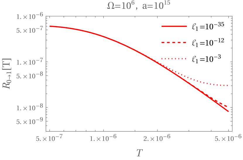
(a)

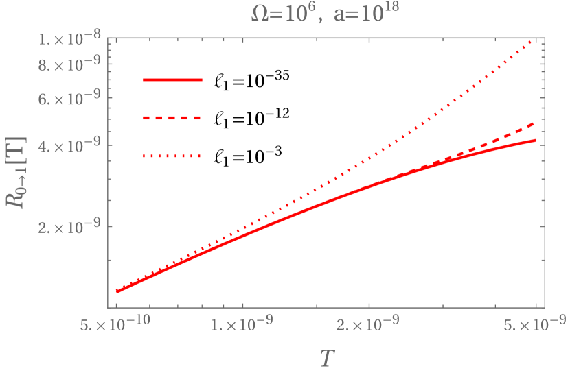
(b)

Figure 2: The transition rate as a function of the width of the window function for different accelerations in Fig. 2(a) and Fig. 2(b), for the shifts of Planck length (solid curve) and macroscopic order (dashed curve). We have used $\bar{m}_{10}^{2}/\hbar^{2}=1$ in these plots.

If the time scale of detector operation is small enough, the second term in Eq. (11) dominantly determines the response, as the first term falls rapidly through its dependency on $T$ (essentially as $\sim(a_{1}\ell_{1})^{1/a_{1}T}$ for small $a_{1}T$ and $a_{1}\ell_{1}<1$), while the fall of the second term is linear w.r.t. $T$. Yet, if the first term becomes completely irrelevant, then the $\ell_{1}$ dependency is again erased, as it survives only in the phase of the inertial-like term. Therefore, there should be a window i.e. $a_{1}T\sim 1$, where both the first and the second term in Eq.(11) are of importance for a macroscopic shift (in fact, the first few sub-leading terms in the series will contribute as well in this case). For the same $T$ if the shift is of the Planck order, then the first term, through its sharp dependence on $\ell_{1}$ in the modulating factor $(a_{1}\ell_{1})^{1/a_{1}T}$, damps down considerably. Thus, for the microscopic shift, only the second term determines the effective response, whereas for the macroscopic shifts, both terms contribute. This, therefore, would lead to a differentiable change in the response of the detector between a large and a small shift, which one can utilize to estimate the difference between the causal domain of two Rindler observers. As discussed in the introduction, a similar computation can be envisaged to estimate the shift of the black hole horizon as seen by two exterior observers before and after the introduction of a mass shell which falls into the black hole. Thus, such a UDW probe can be expected to naturally show up the shift dependency for a finite time operation $1<a_{1}T<a_{1}T_{th}$, where $T_{th}$ is the time detector takes to attain thermal rate.

To illustrate this point with clarity, we integrate the expression in Eq. (11) numerically after restoring the factors of $c$ and $\hbar$ and selecting the parameters such that the tail contribution from the UV sector in the frequency integral can be safely ignored for a suitable cutoff, i.e., $c\omega/a_{1}\rightarrow 10^{10}$. To deal with the IR divergence of the inertial response in $1\oplus 1$ dimension Louko (2014), we also have to employ an IR cutoff. With these choices, we have plotted the transition rate as a function of time for a detector of energy gap $\Omega=10^{6}s^{-1}$ in Fig. 2.

We see that the modulating effects of $\ell_{1}$ start appearing if the detector is kept on for a sufficient duration (microseconds for the acceleration of order $10^{15}ms^{-2}$ and nanoseconds for the acceleration of order $10^{18}ms^{-2}$). Though the numerical accuracy considerations compel us to keep the parameter $T<c/a_{1}$, the trends indicate that the difference in the transition rate for the Planck length shifts and macroscopic shifts keeps on increasing as the detector is kept on for a longer duration, along the expected lines. We anticipate that the difference will reach the maximum for a finite $T$, and the two expressions will merge onto the thermal response for a very large $T$. However, the numerical techniques employed here keep the integral trustworthy for a finite duration, as used in figure 2, which prevents us from locating the extrema. However, even within this allowed range, the response becomes qualitatively apart for the Planck order shifts and macroscopic shifts and the response rate for the microscopic shift is not perturbatively small.

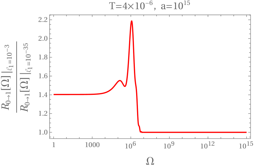
(a)

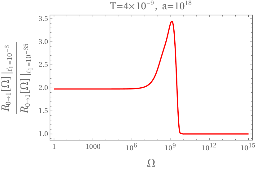
(b)

Figure 3: The ratio of transition rate for the macroscopic shift to the transition rate for Planck shift as a function of the transition frequency with detectors kept on for $T=4\times 10^{-6}s$ and acceleration $a=10^{15}ms^{-2}$ in Fig. 3(a) and detectors kept on for $T=4\times 10^{-9}s$ and with acceleration $a=10^{18}ms^{-2}$ Fig. 3(b). We have used $\bar{m}_{10}^{2}/\hbar^{2}=1$ in these plots.

III.1 Detector Energy Spacing

In order to find an optimal detector for differentiating micro and macro shifts of horizons, we need to identify the domain of the energy gap for which the response, as well as its difference between macroscopic and microscopic shifts, is appreciable for a given acceleration. As discussed earlier, the different responses for different shifts come from the interplay of thermal contribution and series (inertial-like) contribution in (11). The inertial-like contribution is independent of shift, while the thermal term has $(a_{1}\ell_{1})^{2/a_{1}T}$ as a prefactor. From the analytical expression in (11), we see the thermal limit for this detector is when it is switched on for a duration longer than the time scales of the system, i.e., when we have $a_{1}T/c\gg 1$ and $\Omega T\gg 1$. For the parameter regimes that ensure robust numerical analysis in our exploration, the exact thermality is not visible since $a_{1}T/c\leq 1$. However, for large $\Omega$, the inertial-like contribution dominates over the thermal part, which is exponentially suppressed, and thus the response is expected to be independent of the shift. On the other hand, we expect the thermal contribution to increase as $\Omega$ decreases, and at some point, it should become comparable to the inertial-like term and hence of relevance for the total response, thereby making response shift dependent. Thus it indicates that it would be the low energy gap detectors for which the difference between micro and microscopic response gets most pronounced for a given acceleration and switch-on time.

In Fig. 3, we plot the ratio of the transition rate for the macroscopic shift to the microscopic Planck scale shift as a function of the detector energy gap $\Omega$. Regardless of the acceleration of the detector, we see that the ratio is qualitatively different from unity for small $\Omega$ and settles to one for large $\Omega$, as expected. As argued, for $\Omega T\gg 1$, the thermal contribution to the response is negligible for both micro and macroscopic shifts, and the inertial-like term determines the response for both the cases, giving unit value to the ratio. On the other hand, for $\Omega T\leq 1$, the thermal contribution is of the same order as the inertial-like term for the macroscopic shift. In this limit, the thermal contribution for the microscopic shift will be suppressed by a factor $(\ell_{Pl}/\ell_{macro})^{2/a_{1}T}$ compared to the macroscopic shift, hence will become insignificant in total response. Thus, we can see that in the limit $\Omega T\leq 1$, the macroscopic shift response comprises of both the thermal and inertial-like term, both roughly of the similar order, while the microscopic shift response is essentially determined only by the inertial-like term. Therefore, we can expect the macroscopic shift response to be $1-2$ times larger than the microscopic shift case, as indeed can be seen from Fig. 3.

The ratio further attains a maximum near $\Omega T\sim O(1)$, while it settles to a constant value greater than one for $\Omega T\ll 1$. Thus, we find that the Planck order effects become quickly irrelevant for a large transition frequency detectors, i.e., $\Omega T\gg 1$, while the microscopic shifts can be efficiently and distinguishably picked up by detectors with smaller transition frequency with the strongest imprints being in the regime $\Omega T\sim 1$. Therefore, an optimal detector could be one with $a_{1}T\sim c$, which translates to the condition $\Omega c/a_{1}\sim 1$ with the time scale of operation $1/\Omega$. For such detectors, the contrast between a microscopic shift in the causal domain and a macroscopic shift will be most pronounced.

IV Discussion

The problem of quantum fluctuations in spacetime is riddled with problems of small time and small scales. These fluctuations take place over very short time scales and very tiny length scales. Any probe which is expected to capture the imprints of such fluctuations should be sensitive enough to respond to such tiny effects. The issue of short time scales can presumably be taken care of by tuning a probe to the higher moments of fluctuations which survive under macroscopic time averaging. Still, one is left with the issue of designing a sensitive enough probe which can respond to/capture microscopic parameters.

In this work, we attempt to analyze if an Unruh-DeWitt probe on an accelerated trajectory can sense the definitive shift in the causal domain they live in, as compared to that of another Rindler observer. The analysis is motivated by the field theoretic considerations which suggest the global operators, such as number expectations, turn on to a full thermality whenever the Rindler wedges do not completely overlap and mismatch even by the tiniest microscopic shift possible - i.e., the Planck scale Lochan and Padmanabhan (2021). However, such computations require the full spacetime geometry to be completely known beforehand. Thus, it is not very clear if there can be realistic detectors operating in finite regions of spacetime which can respond in the above-mentioned fashion. In this manuscript, we employ a realistic Unruh De Witt detector to analyze the nested system of Rindler frames. We see that the UDW detector, which operates for infinite time responds in a fashion exactly in tune with the number operator expectation. Thus such detectors will respond with a thermal character whenever two accelerated observers do not asymptote to the same null ray in flat space. Though an infinite time detector robustly signals any mismatch in the causal domain of two Rindler observers, it also loses the information about the amount of shift. Thus such detectors can not tell with definiteness if the shift is of Planck scale or macroscopic.

In order to relate with a more realistic experimental set-up, we also compute the response of a finite time detector in this setting. It turns out that a finite time detector on an accelerated trajectory is naturally tuned to capture the tiniest shift in the perceived Rindler horizon compared to any other Rindler wedge. Unlike an infinite time detector, a finite time detector carries a shift dependency in its response which becomes prominent for a detector with energy gap $\Omega c/a\sim 1$ and which operates for time scale $Tc/a\sim 1$ and beyond. For such detectors, the response for a macroscopic shift and microscopic shift are clearly robust and differentiable. It is interesting to note that the response for the Planck shift in both the finite and infinite time detector is of a similar order to that of the Unruh thermality. Therefore, the accelerated detector and fields in the Fock space of any Rindler wedge provide a combination well suited for observing Planck scale shift in the Rindler causal wedges.

It is recently argued that the thermal effect in the UDW detector can be made observationally strong even for moderately small accelerations by employing appropriate boundary conditions Stargen and Lochan (2022). In addition, there are many proposals that try to bring the Unruh effect in the realm of observational verification Crispino et al. (2008). Thus if the Unruh thermality can be efficiently captured in any set-up, it is likely that even the definite Planck scale signatures can also be put to test in those set-ups.

This problem has a potential correspondence with accelerated observers in black hole exterior geometry. Since the analysis really scrutinizes if two accelerated observers will asymptotically approach the same null ray or not, it can be employed between two exterior observers in the exterior of a black hole geometry in which one of the observers asymptotically approaches the event horizon while the other just crosses over due to the growth of the horizon caused by an in-fall of some microscopic mass. Thus one needs to generalize these computations to a curvature-full and more realistic $3\oplus 1$ dimensional spacetime. Moreover, even the field theoretic computations should be generalized for such finite time operations to gain insights if the emission from the black hole also contains rich information of its horizon shift. In the context of cosmology, similar analysis may potentially address the effects revealing shifts in cosmological horizons due to the expansion of the universe. These analyses will hopefully be performed in subsequent studies.

V Acknowledgemnt

Research of KL is partially supported by SERB, Govt. of India through a MATRICS research grant no. MTR/2022/000900. HSS would like to acknowledge the financial support from the University Grants Commission, Government of India, in the form of Junior Research Fellowship (UGC-CSIR JRF/Dec-2016/503905).

Appendix A Derivation of finite time detector response

In this section, we derive the expression for the transition probability for the detector that is switched on for a finite time and check the robustness of the result for different physical scenarios. The integral of interest is Eq. (9)

$$I_{1}(\omega)=\int_{-\infty}^{\infty}dk\;\tilde{\chi}(k)\int_{-\infty}^{\infty}d\tau\;e^{-i\left(\Omega+\omega\frac{a_{1}}{a_{0}}-k\right)\tau}\left(1+a_{1}\ell_{1}e^{a_{1}\tau}\right)^{i\frac{\omega}{a_{0}}},$$ (12)

where $\tilde{\chi}(k)$ is the Fourier transform of the window function. For the case of a window function with exponential cutoff $\chi(t)=e^{-|t|/T}$, we have

$$\tilde{\chi}(k)=\frac{T}{\pi(1+k^{2}T^{2})}.$$ (13)

The time integral in Eq. (12) can be solved using the result Oberhettinger (1990)

$$\int_{-\infty}^{\infty}dx\;e^{(\epsilon+ip)x}(1+Ae^{x})^{-\epsilon_{2}-iq} =\frac{A^{-\epsilon-ip}\Gamma(\epsilon_{1}+i(q-p))\Gamma(\epsilon+ip)}{\Gamma(\epsilon_{2}+iq)},$$ (14)

where $p\;\&\;q\;\in\;\mathbb{R}$ and the regulators behave as $0<\epsilon_{1}<\epsilon_{2}$ and $\epsilon_{2}-\epsilon_{1}=\epsilon>0$. The regulators in this analysis are of particular importance, and by retaining these, we arrive at

$$I_{1}(\omega)=\frac{T}{\pi}\int_{-\infty}^{\infty}dk\;\frac{(a_{1}\ell_{1})^{-\epsilon_{1}+i\left(\frac{\Omega-k}{a_{1}}+\frac{\omega}{a_{0}}\right)}\Gamma\left(\epsilon_{2}-\epsilon_{1}+i\frac{\Omega-k}{a_{1}}\right)\Gamma\left(\epsilon_{1}-i\left(\frac{\Omega-k}{a_{1}}+\frac{\omega}{a_{0}}\right)\right)}{a_{1}(1+k^{2}T^{2})\Gamma\left(\epsilon_{2}-i\frac{\omega}{a_{0}}\right)}.$$ (15)

This integration can be solved by using the residue theorem, in which the regulators determine the location of the poles. It is convenient to work with

$$I_{1}(\omega) =-\frac{i\;T(a_{1}\ell_{1})^{i\left(\frac{\Omega}{a_{1}}+\frac{\omega}{a_{0}}\right)}}{\pi\Gamma\left(\epsilon_{2}-i\frac{\omega}{a_{0}}\right)}\int_{-i\infty}^{i\infty}dx(a_{1}\ell_{1})^{-x}\frac{1}{1-a_{1}^{2}x^{2}T^{2}}\Gamma\left(\epsilon_{2}-\epsilon_{1}+i\frac{\Omega}{a_{1}}-x\right)\Gamma\left(\epsilon_{1}-i\left(\frac{\Omega}{a_{1}}+\frac{\omega}{a_{0}}\right)+x\right)$$ (16)

$$=-\frac{i\;T(a_{1}\ell_{1})^{i\left(\frac{\Omega}{a_{1}}+\frac{\omega}{a_{0}}\right)}}{\pi\Gamma\left(\epsilon_{2}-i\frac{\omega}{a_{0}}\right)}\int_{-i\infty}^{i\infty}dx(a_{1}\ell_{1})^{-x}\frac{1}{1-a_{1}^{2}x^{2}T^{2}}\Gamma\left(\beta-x\right)\Gamma\left(\alpha+x\right).$$ (17)

The direction of the closure of the contour is determined by whether $a_{1}\ell_{1}>1$ or $a_{1}\ell_{1}<1$ in order to satisfy Jordan’s lemma. In the first case, the contour is closed from $Re(x)>0$, and in the second case, from $Re(x)<0$. In this analysis, we are interested in the shifts of extremely small magnitude; therefore, the second case is preferred. We can arrive at the expression for the first case following the same derivation. The poles of the integrand are at

$$\Gamma(\alpha+x) :\qquad\alpha+\alpha_{n}=-n\implies\alpha_{n}=-n-\alpha;\qquad\forall\;n\;\in\mathbb{N}_{0},$$ (18)

$$\Gamma(\beta-x) :\qquad\beta-\beta_{n}=-n\implies\beta_{n}=n+\beta,$$ (19)

$$\frac{1}{1-a_{1}^{2}x^{2}T^{2}} :\qquad x_{\pm}=\pm\frac{1}{a_{1}T}.$$ (20)

Residues at respective poles are

$$\alpha_{n}: \qquad Res_{\alpha_{n}}=\frac{(-1)^{n}(a_{1}\ell_{1})^{\alpha+n}\Gamma(\alpha+\beta+n)}{(1-a_{1}^{2}T^{2}(\alpha+n)^{2})n!},$$ (21)

$$\beta_{n}: \qquad Res_{\beta_{n}}=\frac{(-1)^{n+1}(a_{1}\ell_{1})^{-\beta-n}\Gamma(\alpha+\beta+n)}{(1-a_{1}^{2}T^{2}(\beta+n)^{2})n!},$$ (22)

$$x_{\pm}: \qquad Res_{\pm}=\mp(a_{1}\ell_{1})^{\mp\frac{1}{a_{1}T}}\frac{\Gamma\left(\beta\mp\frac{1}{a_{1}T}\right)\Gamma\left(\alpha\pm\frac{1}{a_{1}T}\right)}{2a_{1}T}.$$ (23)

Figure 4: Contour relevant for the case when $a_{1}\ell_{1}<1$. The residues of poles at red points contribute in this case, whereas the residues of poles at blue points contribute in the case of $a_{1}\ell_{1}>1$

In the case of $a_{1}\ell_{1}<1$, the relevant contour is a closed loop consisting of the imaginary axis and the semicircular arc of infinite radius on the left side, $C_{\infty}\cup\mathbb{R}$. The poles that are enclosed in the contour are $\alpha_{n}$ and $x_{-}$, and the contour integral is given by

$$\oint dx(a_{1}\ell_{1})^{-x}\frac{1}{1-a_{1}^{2}x^{2}T^{2}}\Gamma\left(\beta-x\right)\Gamma\left(\alpha+x\right)=2\pi i\left(\sum_{n=0}^{\infty}Res_{\alpha_{n}}+Res_{x_{-}}\right).$$ (24)

The integral along the semicircular arc $C_{\infty}$ vanishes following Jordan’s lemma, and therefore the integral of interest takes the form

$$I_{1}(\omega)=\frac{2T(a_{1}\ell_{1})^{i\left(\frac{\Omega}{a_{1}}+\frac{\omega}{a_{0}}\right)}}{\Gamma\left(\epsilon_{2}-i\frac{\omega}{a_{0}}\right)}\left[\sum_{n=0}^{\infty}\left(\frac{(-1)^{n}(a_{1}\ell_{1})^{\alpha+n}\Gamma(\alpha+\beta+n)}{(1-a_{1}^{2}T^{2}(\alpha+n)^{2})n!}\right)+\frac{(a_{1}\ell_{1})^{\frac{1}{a_{1}T}}\Gamma\left(\beta+\frac{1}{a_{1}T}\right)\Gamma\left(\alpha-\frac{1}{a_{1}T}\right)}{2a_{1}T}\right].$$ (25)

Since $|I_{1}(\omega)|^{2}$ appears in the expression of transition probability, we omitted the outside phase factor in the main text. At this point, we can take the limit $\epsilon_{1/2}\rightarrow 0$ in the expressions. The first thing we will check is the convergence of infinite series.

$$\lim_{n\rightarrow\infty}\left|\frac{Res_{\alpha_{n+1}}}{Res_{\alpha_{n}}}\right| =\lim_{n\rightarrow\infty}\left|\frac{(-1)^{n+1}(a_{1}\ell_{1})^{\alpha+n+1}\Gamma(\alpha+\beta+n+1)}{(1-a_{1}^{2}T^{2}(\alpha+n+1)^{2})(n+1)!}\frac{(1-a_{1}^{2}T^{2}(\alpha+n)^{2})n!}{(-1)^{n}(a_{1}\ell_{1})^{\alpha+n}\Gamma(\alpha+\beta+n)}\right|$$ (26)

$$=\lim_{n\rightarrow\infty}\left|-\frac{a_{1}\ell_{1}(\alpha+\beta+n)(1-a_{1}^{2}T^{2}(\alpha+n)^{2})}{(1-a_{1}^{2}T^{2}(\alpha+n+1)^{2})(n+1)}\right|=|a_{1}\ell_{1}|<1.$$ (27)

Therefore, the series converges according to Cauchy’s ratio test. Next, we check the consistency of the result obtained under different physical limits.

A.1 Eternal and instantaneous switching limit

In the $T\rightarrow\infty$ limit, the window function becomes unity, representing the case of eternal switching, and one expects to recover the infinite-time result. For this limit, each term in the infinite series in Eq. (25) behaves as $T^{-1}$ and thus vanishes. The last term in the Eq. (25)

$$\lim_{T\rightarrow\infty}I_{1}(\omega)=\lim_{T\rightarrow\infty}\frac{(a_{1}\ell_{1})^{\frac{1}{a_{1}T}}\Gamma\left(i\frac{\Omega}{a_{1}}+\frac{1}{a_{1}T}\right)\Gamma\left(-i\left(\frac{\Omega}{a_{1}}+\frac{\omega}{a_{0}}\right)-\frac{1}{a_{1}T}\right)}{a_{1}\Gamma\left(-i\frac{\omega}{a_{0}}\right)}=\frac{\Gamma\left(i\frac{\Omega}{a_{1}}\right)\Gamma\left(-i\left(\frac{\Omega}{a_{1}}+\frac{\omega}{a_{0}}\right)\right)}{a_{1}\Gamma\left(-i\frac{\omega}{a_{0}}\right)}$$ (28)

which will give us the thermal response. At the other asymptotic limit $T\rightarrow 0$, the window function is sharply peaked at the origin, and we expect the transition probability to vanish. Again, the infinite series is proportional to $T$ in this limit and therefore vanishes. The relevant asymptotic expressions are

$$\left|\Gamma\left(i\frac{\Omega}{a_{1}}+\frac{1}{a_{1}T}\right)\Gamma\left(-i\left(\frac{\Omega}{a_{1}}+\frac{\omega}{a_{0}}\right)-\frac{1}{a_{1}T}\right)\right|^{2}\xrightarrow{T\rightarrow 0}\left|\pi a_{1}T\csc\left[\pi\left(-\frac{1}{a_{1}T}-i\left(\frac{\omega}{a_{0}}+\frac{\Omega}{a_{1}}\right)\right)\right]\right|^{2}.$$ (29)

For the last term in Eq. (25), we have

$$\lim_{T\rightarrow 0}|I(\omega)|^{2} =\lim_{T\rightarrow 0}\left|\frac{(a_{1}\ell_{1})^{\frac{1}{a_{1}T}}\Gamma\left(i\frac{\Omega}{a_{1}}+\frac{1}{a_{1}T}\right)\Gamma\left(-i\left(\frac{\Omega}{a_{1}}+\frac{\omega}{a_{0}}\right)-\frac{1}{a_{1}T}\right)}{a_{1}\Gamma\left(-i\frac{\omega}{a_{0}}\right)}\right|^{2}$$ (30)

$$=\lim_{T\rightarrow 0}\left|\frac{\pi T(a_{1}\ell_{1})^{\frac{1}{a_{1}T}}\csc\left[\pi\left(-\frac{1}{a_{1}T}-i\left(\frac{\omega}{a_{0}}+\frac{\Omega}{a_{1}}\right)\right)\right]}{\Gamma\left(-i\frac{\omega}{a_{0}}\right)}\right|^{2}$$ (31)

Since $a_{1}\ell_{1}<1$, the term $(a_{1}\ell_{1})^{1/T}$ is decaying exponentially whereas the $\csc$ term is highly oscillating but with finite amplitude as $T\rightarrow 0$. Therefore, the transition probability vanishes in this case.

A.2 Vanishing shift limit

In the limit of the vanishing shift, the thermal equivalence is lost, and we expect the inertial response in this case. With the window function under consideration, the response of a detector on the inertial trajectory for the same window function is given by

$$P_{0\rightarrow 1}=\frac{\bar{m}_{10}^{2}}{2\pi}\int^{\infty}_{0}\frac{d\omega}{\omega}\frac{4T^{2}}{(1+(\Omega+\omega(1-v)\gamma)^{2}T^{2})^{2}}.$$ (32)

Here, $v$ is the velocity of the detector, and $\gamma$ is the Lorentz factor. On the other hand, all terms in Eq. (25) vanish except for the leading-order term in infinite series in the limit of $\ell_{1}\rightarrow 0$.

$$I_{1}(\omega)=\lim_{\ell_{1}\rightarrow 0}\frac{2T(a_{1}\ell_{1})^{i\left(\frac{\Omega}{a_{1}}+\frac{\omega}{a_{0}}\right)}}{\Gamma\left(\epsilon_{2}-i\frac{\omega}{a_{0}}\right)}\left(\frac{(a_{1}\ell_{1})^{\alpha}\Gamma(\alpha+\beta)}{(1-a_{1}^{2}T^{2}\alpha^{2})}\right).$$ (33)

With $\alpha=-i(\Omega/a_{1}+\omega/a_{0})$ and $\beta=i\Omega/a_{1}$, the above expression reduces to

$$I_{1}(\omega)=\frac{2T}{1+a_{1}^{2}T^{2}\left(\frac{\Omega}{a_{1}}+\frac{\omega}{a_{0}}\right)^{2}}.$$ (34)

Using this, the transition probability is given by

$$P_{0\rightarrow 1}=\bar{m}_{10}^{2}\int^{\infty}_{0}\frac{d\omega}{2\pi\omega}\frac{4T^{2}}{\left(1+T^{2}\left(\Omega+\frac{a_{1}\omega}{a_{0}}\right)^{2}\right)^{2}}.$$ (35)

The transition probability, in this case, has qualitative features of the inertial case, with the ratio of accelerations of different Rindler frames $a_{1}/a_{0}$ playing the role of factor $(1-v)\gamma=\sqrt{(1-v)/(1+v)}$. Since the system is $1\oplus 1$ dimensional scalar field, the transition probability has IR divergence, related to the IR ambiguity in the Wightman function of a scalar field in $1\oplus 1$ dimensions Louko (2014). In our analysis, we introduce an arbitrary IR cutoff to deal with the divergence. Thus, we see that the infinite series contributes to the inertial part of the response, and the second term in Eq. (25) contributes to the thermal part of the response.

Appendix B Convergence of the finite time response

In this section, we discuss the convergence of the integral appearing in the finite time response in Eq. (11). First, the inertial response has IR divergence as seen in the integral in Eq. (35), which is related to the IR ambiguity in the Wightman function of the scalar field in $1\oplus 1$ dimension Louko (2014). To numerically integrate, we are introducing an IR cutoff which leads to a finite inertial response. For the thermal part of the response, the integral of interest is

$$I(T,\Omega,a_{1})=\left|\Gamma\left(i\frac{\Omega}{a_{1}}+\frac{1}{a_{1}T}\right)\right|^{2}\int_{0}^{\infty}\frac{d\tilde{\omega}}{2\pi\tilde{\omega}}\left|\frac{\Gamma\left(-i\left(\frac{\Omega}{a_{1}}+\tilde{\omega}\right)-\frac{1}{a_{1}T}\right)}{a_{1}\Gamma\left(-i\tilde{\omega}\right)}\right|^{2},$$ (36)

where we have rescaled the integration variable $\omega$. The asymptotic behavior of the integrand at the limits of integration is

$$\lim_{\tilde{\omega}\rightarrow 0}\frac{1}{\tilde{\omega}}\left|\frac{\Gamma\left(-i\left(\frac{\Omega}{a_{1}}+\tilde{\omega}\right)-\frac{1}{a_{1}T}\right)}{\Gamma\left(-i\tilde{\omega}\right)}\right|^{2} =\left|\Gamma\left(-i\frac{\Omega}{a_{1}}-\frac{1}{a_{1}T}\right)\right|^{2}\tilde{\omega}(1+O(\tilde{\omega})),$$ (37)

$$\lim_{\tilde{\omega}\rightarrow\infty}\frac{1}{\tilde{\omega}}\left|\frac{\Gamma\left(-i\left(\frac{\Omega}{a_{1}}+\tilde{\omega}\right)-\frac{1}{a_{1}T}\right)}{\Gamma\left(-i\tilde{\omega}\right)}\right|^{2} =\tilde{\omega}^{-1-1/2a_{1}T}\left(e^{-\pi\Omega/a_{1}}+O(\tilde{\omega}^{-1})\right).$$ (38)

For the case at hand, the integrand has the appropriate behavior at both limits for the integral to converge. The integral is logarithmically divergent at the limit of $T\rightarrow\infty$, as explicitly shown in Lochan and Padmanabhan (2021). Although the falloff of the tail of the integrand for finite $T$ and large $\omega$ is faster than $\omega^{-1}$, one still has to be careful when numerically integrating it.

Ideally, for an improper integral with the upper limit as infinite, one needs to identify a cutoff beyond which the contribution of the area under the tail can be neglected. For the behavior of the integrand under consideration, such a universal cutoff $\omega_{o}$ does not exist. In fact, the cutoff in this case is highly sensitive to $a_{1}$ and $T$, as these parameters appear in the exponent in Eq. (38). The strategy we will employ here is, to identify the window of the parameter $T$ for a particular acceleration, for which we can trust the numerical results with an appropriate cutoff.

Appendix C Ambiguity in defining finite time response

The transition rate can be defined by either dividing the transition probability by the time detector is swiched on or by taking the time derivative of transition probability. In the limit $T\rightarrow\infty$, these two notions are expected to agree. In this appendix, we estimate the difference in two prescriptions for the finite $T$ case. For simplicity, we consider the case of thermal contribution to the response only and restoring the factors of $c$ and $\hbar$, the two notions of transition rate are given by

$$R^{1}_{0\rightarrow 1}(\Omega,a_{1},T) =\frac{\bar{m}_{10}^{2}}{\hbar^{2}T}\left(\frac{a_{1}\ell_{1}}{c^{2}}\right)^{\frac{2c}{a_{1}T}}\int_{0}^{\infty}\frac{d\omega}{2\pi\omega}\left|\frac{c\Gamma\left(i\frac{\Omega c}{a_{1}}+\frac{c}{a_{1}T}\right)\Gamma\left(-i\left(\frac{\Omega c}{a_{1}}+\frac{\omega c}{a_{0}}\right)-\frac{c}{a_{1}T}\right)}{a_{1}\Gamma\left(-i\frac{\omega c}{a_{0}}\right)}\right|^{2},$$ (39)

$$R^{2}_{0\rightarrow 1}(\Omega,a_{1},T) =\frac{\bar{m}_{10}^{2}}{\hbar^{2}}\frac{d}{dT}\left[\left(\frac{a_{1}\ell_{1}}{c^{2}}\right)^{\frac{2c}{a_{1}T}}\int_{0}^{\infty}\frac{d\omega}{2\pi\omega}\left|\frac{c\Gamma\left(i\frac{\Omega c}{a_{1}}+\frac{c}{a_{1}T}\right)\Gamma\left(-i\left(\frac{\Omega c}{a_{1}}+\frac{\omega c}{a_{0}}\right)-\frac{c}{a_{1}T}\right)}{a_{1}\Gamma\left(-i\frac{\omega c}{a_{0}}\right)}\right|^{2}\right].$$ (40)

We have plotted the transition rate as a function of the width of the window function and the transition frequency in Fig. 5. For both definitions of transition rate, the functional dependence is the same, although the magnitude is larger for the case of (40).

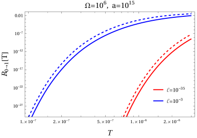
Figure 5: The thermal contribution to the transition rate as a function of the width of the window function for the shifts of Planck length (red curves) and macroscopic order (blue curves). Here, the solid profiles correspond to the response rate defined in Eq. (39), and the dashed profiles correspond to the response rate defined in Eq. (40). We have used $\bar{m}_{10}^{2}/\hbar^{2}=10^{6}$ in these plots.

References

- Lochan and Padmanabhan (2021) K. Lochan and T. Padmanabhan, (2021), arXiv:2107.03406 [gr-qc] .
- Percival (1995) I. C. Percival, Proc. Roy. Soc. Lond. A 451, 503 (1995), arXiv:quant-ph/9508021 .
- Hu and Verdaguer (2004) B. L. Hu and E. Verdaguer, Living Rev. Rel. 7, 3 (2004), arXiv:gr-qc/0307032 .
- Salecker and Wigner (1958) H. Salecker and E. P. Wigner, Phys. Rev. 109, 571 (1958).
- Husain and Louko (2016) V. Husain and J. Louko, Phys. Rev. Lett. 116, 061301 (2016), arXiv:1508.05338 [gr-qc] .
- Ford (1995) L. H. Ford, Phys. Rev. D 51, 1692 (1995), arXiv:gr-qc/9410047 .
- Ford and Svaiter (1997) L. H. Ford and N. F. Svaiter, Phys. Rev. D 56, 2226 (1997), arXiv:gr-qc/9704050 .
- Thompson and Ford (2008) R. T. Thompson and L. H. Ford, Phys. Rev. D 78, 024014 (2008), arXiv:0803.1980 [gr-qc] .
- Mathur (2005) S. D. Mathur, Fortsch. Phys. 53, 793 (2005), arXiv:hep-th/0502050 .
- Chakraborty and Lochan (2017) S. Chakraborty and K. Lochan, Universe 3, 55 (2017), arXiv:1702.07487 [gr-qc] .
- Unruh (1976) W. G. Unruh, Phys. Rev. D 14, 870 (1976).
- Kajuri (2016) N. Kajuri, Class. Quant. Grav. 33, 055007 (2016), arXiv:1508.00659 [gr-qc] .
- Birrell and Davies (1984) N. D. Birrell and P. C. W. Davies, Quantum Fields in Curved Space, Cambridge Monographs on Mathematical Physics (Cambridge Univ. Press, Cambridge, UK, 1984).
- Oberhettinger (1990) F. Oberhettinger, Tables of Fourier Transforms and Fourier Transforms of Distributions (Springer Berlin Heidelberg, 1990) pp. 204, Chapter 3.
- Svaiter and Svaiter (1992) B. F. Svaiter and N. F. Svaiter, Phys. Rev. D 46, 5267 (1992), [Erratum: Phys.Rev.D 47, 4802 (1993)].
- Sriramkumar and Padmanabhan (2002) L. Sriramkumar and T. Padmanabhan, Int. J. Mod. Phys. D 11, 1 (2002), arXiv:gr-qc/9903054 .
- Louko and Satz (2006) J. Louko and A. Satz, Class. Quant. Grav. 23, 6321 (2006), arXiv:gr-qc/0606067 .
- Sriramkumar and Padmanabhan (1996) L. Sriramkumar and T. Padmanabhan, Class. Quant. Grav. 13, 2061 (1996), arXiv:gr-qc/9408037 .
- Louko (2014) J. Louko, JHEP 09, 142 (2014), arXiv:1407.6299 [hep-th] .
- Stargen and Lochan (2022) D. J. Stargen and K. Lochan, Phys. Rev. Lett. 129, 111303 (2022), arXiv:2107.00049 [gr-qc] .
- Crispino et al. (2008) L. C. B. Crispino, A. Higuchi, and G. E. A. Matsas, Rev. Mod. Phys. 80, 787 (2008), arXiv:0710.5373 [gr-qc] .