Rotation at the Fully Convective Boundary: Insights from Wide WD + MS Binary Systems

Abstract

Gyrochronology, a valuable tool for determining ages of low-mass stars where other techniques fail, relies on accurate calibration. We present a sample of 327 wide ($>$$100$ au) white dwarf + main sequence (WD + MS) binary systems. Total ages of WDs are computed using all-sky survey photometry, Gaia parallaxes, and current hydrogen atmosphere WD models. Using a magnetic braking law calibrated against open clusters, along with assumptions about initial conditions and angular momentum transport, we construct gyrochrones to predict the rotation periods of the MS stars. Both data and models show that, near the fully convective boundary, MS stars with WD ages up to 7.5 Gyr experience a rotation period increase by up to a factor of $\approx$$3$ within a $<50\,\mathrm{K}$ effective temperature range. We suggest that rapid braking at this boundary is driven by a sharp rise in the convective overturn timescale ($\tau_{\mathrm{cz}}$) caused by structural changes between partially and fully convective stars and the ${}^{3}\textrm{He}$ instability occurring at this boundary. While the specific location in mass (or temperature) of this feature varies with model physics, we argue that its existence remains consistent. Stars along this feature exhibit rotation periods that can be mapped, within 1$\sigma$, to a range of gyrochrones spanning $\approx 6$  Gyr. Due to current temperature errors ($\simeq$$50\,\mathrm{K}$), this implies that a measured rotation period cannot be uniquely associated to a single gyrochrone, implying that gyrochronology may not be feasible for M dwarfs very close to the fully convective boundary.

1 Introduction

Ages of stars are critical to our understanding of the evolution of astrophysical systems and yet are one of the most difficult stellar properties to measure. The only star for which we have a precise and accurate age is the Sun; for any other star, age can only be estimated or inferred. There are many techniques to estimate stellar ages, but there is no single method that is applicable to all spectral types (Soderblom, 2010).

K and M dwarfs are the most numerous stars in the Galaxy and have lifetimes longer than the age of the Milky Way disk, meaning that they preserve a record of the history of star formation and chemical evolution of the Galaxy. They are, however, resistant to standard age-dating techniques. Isochrone fitting fails to provide constraints on stellar ages when used on low-mass stars, due to their slow nuclear evolution (Takeda et al., 2017). Similarly, asteroseismology, which provides precise ages for Sun-like stars, cannot be used to date low-mass stars like K and M dwarfs due to their low oscillation amplitudes (Chaplin et al., 2011).

A promising tool in this low mass regime is gyrochronology (Barnes, 2007), which derives ages for cool MS stars by exploiting the fact that they spin down with time (Skumanich, 1972) due to magnetic braking. Magnetic braking is the mechanism by which a star loses angular momentum to magnetized stellar winds over time as the result of the interaction between mass loss and dynamo-driven stellar magnetic fields. Epstein & Pinsonneault (2014) showed that under Skumanich-type spin down, rotation-based age dating is potentially among the most precise methods available.

Calibration of period-age relations for low mass stars requires a large sample of old, well-dated low mass stars. However, only a handful of stars below 0.8 $M_{\odot}$ are currently available, and most of them are in young clusters (4 Gyr at the oldest, Dungee et al., 2022). Furthermore, observations of these clusters have shown that standard braking models fail to reproduce the observed rotational sequences, suggesting that stellar spin-down may not be as simple as it once appeared.

Recent measurements of the rotation period ($P_{\mathrm{rot}}$) of stars in the benchmark open clusters Praesepe ($\approx$700 Myr, Douglas et al., 2019) and NGC 6811 (1Gyr, Meibom et al., 2011; Janes et al., 2013) show that a simple power law with a braking index $n$ ($n=0.5$ in the Skumanich law) fails at predicting the observed rotational sequences in these clusters (Curtis et al., 2020). While solar-type stars in NGC 6811 have longer periods compared to their counterparts in the younger cluster Praesepe, the two sequences merge at $M<0.8$ $M_{\odot}$ (K0 to M0-type stars, Curtis et al., 2019; Douglas et al., 2019). In other words, the spin-down appears to “stall” (or reduce) for low-mass stars in NGC 6811. Spada & Lanzafame (2020) demonstrated that this phenomenon can be explained by relaxing the assumption of solid-body rotation and allowing for angular momentum (AM) transport between the core and the envelope (i.e. radial differential rotation). The spin-down stalling observed in K and early M-type stars in NGC 6811 is putatively an epoch when AM transport from the core to the envelope balances the AM loss at the surface due to winds. The lack of a radiative core in fully convective stars that can support such core-envelope interaction may be responsible for the closure of the intermediate period gap discovered with Kepler by McQuillan et al. (2013) at the fully convective boundary (Lu et al., 2021).

Near the fully convective boundary, another relevant feature is the underdensity of stars observed near $M_{G}=10.2$ in the main sequence on the Hertzsprung-Russell diagram found by Jao et al. (2018) using Gaia DR2 measurements. It has been proposed that this Gaia M-dwarf gap is a manifestation of the location where stars transition from partially to fully convective, which is predicted to occur at a mass of $\sim 0.35$ $M_{\odot}$. Earlier theoretical work by van Saders & Pinsonneault (2012a) demonstrated that stars slightly above this threshold undergo a structural instability due to non-equilibrium ³He burning during the first few billion years on the main sequence. This results in the development of a convective core, separated from a deep convective envelope by a thin radiative layer. The continuous accumulation of central ³He causes the radiative zone separating them to thin even further, initiating fully convective episodes. Using stellar models and stellar population synthesis, Feiden et al. (2021) confirmed that the ³He instability is responsible for the appearance of the M-dwarf gap.

With the distinct structural changes across the fully convective boundary, there have been attempts to comprehend whether there are any consequences for the magnetic properties, activity levels, and rotation rates of stars. For instance, Donati et al. (2008) and Reiners & Basri (2009) demonstrated that $0.34-0.36$ $M_{\odot}$ stars are prone to undergo sudden alterations in their large-scale magnetic topologies, which could lead to observable surface activity signatures. More recently, Jao et al. (2023) conducted a high-resolution spectroscopic H$\alpha$ emission survey of M dwarfs spanning the Gaia M-dwarf gap and argued that stars above the top gap edge exhibit H$\alpha$ emission while stars within the gap or below do not display any emission. Thus, stars near the fully convective boundary provide a powerful laboratory for testing the physics of M-dwarf stars, including those affected by the ³He instability. Moreover, having a reliable spin-down model that can predict the rotational evolution of these stars is crucial for determining a precise period-age relation for old, low-mass stars.

A primary limitation is the lack of empirical anchors of known age for old K and M-type stars. Open clusters have been the major contributors of calibrators to date; however, due to their short dissipation timescales ($\sim$200 Myr; Wielen, 1971), old clusters are rare and tend to be more distant and challenging to observe. The standard gyrochronology calibrators and the recent observations of late K- and early M- dwarfs in M67 (Dungee et al., 2022) do not extend beyond 4 Gyr for stars below 0.8 $M_{\odot}$. Likewise, the asteroseismic calibrator sample that has been important for understanding braking in solar-mass stars (van Saders et al., 2016; Hall et al., 2021) does not extend beyond $\approx 0.8$ $M_{\odot}$.

Wide binaries that contain a white dwarf (WD) companion provide a distinctive opportunity to determine the ages of field stars. WDs are the end product of stars with initial masses less than $8-10$ $M_{\odot}$ and, as they no longer undergo nuclear fusion in their core, they gradually cool with time becoming dimmer and colder. Because their effective temperature and mass uniquely correspond to a single cooling age (given a composition), WDs have been utilized as stellar clocks for decades (Fontaine et al., 2001). The advancement of robust cooling models (Bergeron et al., 1995) allows WDs to serve as precise and dependable age indicators. However, to determine the complete age of a WD, one needs to consider the time from its zero-age main sequence (ZAMS) to its present state as a WD. This involves using a semi-empirical initial-final mass relation (IFMR) in conjunction with stellar evolution model grids to ascertain the progenitor lifetimes from the ZAMS to the WD phase. Using photometry only, Heintz et al. (2022) found that WD ages are precise at the 25% level for WDs with masses $>0.63\,M_{\odot}$.

Wide, coeval binaries are sufficiently distant ($>100$ au) that the two stars can be expected to evolve as single stars without any interaction between them (White & Ghez, 2001). Therefore, the WD companion offers an independent age estimate of the entire system, making it possible to extend period-age relationships to the age of the galactic disk for the most common stars in our galaxy.

The number of wide coeval binary systems has significantly increased since the launch of the Gaia spacecraft. From Gaia DR2, El-Badry & Rix (2018) constructed a catalog of over $\sim$$53{,}000$ binaries, $\sim$$3000$ of which contained a WD and a main sequence star, which represented a tenfold increase in the number of known coeval binaries (Holberg et al., 2013). With the release of Gaia eDR3, El-Badry et al. (2021) published an extensive catalog of 1.3 million spatially resolved binary stars within $\approx$$1$ kpc of the Sun, including more than $16{,}000$ WD + MS binaries, which increased the sample by another order of magnitude. This increase presents an opportunity to infer precision ages for cool, old stars, which are the focus of this work.

In Section 2 we describe the physics of the rotational evolution models, their calibration and the technique used to determine WD ages. In Section 3, we present the sample selection of WD + MS systems. The ages of these systems as revealed by our models and WDs are discussed in Section 4, where we also compare our sample to other datasets. Finally, the conclusions of our results are presented in Section 5.

2 Methods

2.1 Gyrochronology Models

We use the rotation code rotevol (van Saders & Pinsonneault, 2013; Somers et al., 2017) to model the AM evolution of a star. We use as input non-rotating tracks with stellar masses between 0.18 and 1.15 M_⊙, generated using the Yale Rotating Evolution Code (YREC, see van Saders & Pinsonneault, 2012b; Pinsonneault et al., 1989; Bahcall & Pinsonneault, 1992). The models include helium and heavy element diffusion following Thoul et al. (1994), but with the diffusion coefficients multiplied by a factor of 0.753 to match the helioseismically determined helium abundance (Basu & Antia, 1995) in the Sun at solar age. We adopt boundary conditions using the Allard et al. (1997) atmospheric tables, OPAL opacities (Iglesias & Rogers, 1996) with low-temperature opacities from Ferguson et al. (2005) for a Grevesse & Sauval (1998) solar mixture. We adopt nuclear reaction rates from Adelberger et al. (2011) with weak screening (Salpeter, 1954) and the equation of state from the OPAL project (Rogers et al., 1996; Rogers & Nayfonov, 2002). We assume no overshooting, and a mixing length theory of convection (Cox & Giuli, 1968; Vitense, 1953). Our solar-calibrated model at 4.57 Gyr (Bahcall et al., 1995) has $Z=0.01709$, $X=0.71642$ and mixing length parameter $\alpha_{ml}=1.94243$. We run models at a range of surface spot covering fractions in YREC (0%, 25% and 50%) following the prescription of Somers & Pinsonneault (2015) and Somers et al. (2020) with $x_{spot}=0.8$ but retain otherwise identical physical ingredients in the spotted models.

We run YREC in the non-rotating configuration and compute the rotational evolution post hoc using the tracer code rotevol (van Saders & Pinsonneault, 2013; Somers et al., 2017). The benefit of this approach is that we can rapidly search parameter space when fitting the magnetic braking law to the observations; the downside is that rotation cannot influence the structure. While this is a reasonable assumption for all but the most rapid rotators, ideally one would actively couple the starspot filling fraction to the rotation rate (e.g. Cao & Pinsonneault, 2022; Cao et al., 2023). We leave this exercise to future work, and instead examine the behavior of a range of fixed spot covering fractions.

To model the rotation period evolution of a star as a function of time, one must choose appropriate initial starting conditions as well as to specify prescriptions for three processes that drive the angular momentum (AM) evolution, early disk interactions, AM loss at the stellar surface through magnetized winds (“braking law”), and internal AM transport. In this section, we describe the ingredients and assumptions of the stellar evolutionary models.

2.1.1 Initial conditions

The rotation period $(P_{\mathrm{rot}})$ of a star approaching the MS is determined largely by two factors: the initial rotation period $(P_{\mathrm{init}})$ and the protostellar disk lifetime $(\tau_{\mathrm{disk}})$. Observations of stars in young clusters indicate both that there is a strong mass-rotation correlation in the $P_{\mathrm{init}}$ distribution for low-mass stars and that stars at a fixed mass can have a wide range of initial rotation rates (e.g. Somers et al., 2017). This variation in initial rotation conditions results in a range of rotation periods (approximately $\approx$ 0.1 to 10 days) when stars reach the zero age main-sequence (ZAMS). Although initial conditions become less significant for older stars (van Saders & Pinsonneault, 2013; Epstein & Pinsonneault, 2014; Bouvier, 2013), there are certain combinations of stellar ages and masses, namely the K and M dwarfs of interest, where this initial variability is important (Bouvier, 2013; Gallet & Bouvier, 2015).

The models start on the pre-MS, where the distribution of initial rotation conditions is set up by the young cluster Upper Sco at 10 Myr. By this age massive accretion disks are nearly absent (Williams & Cieza, 2011) and significant AM loss has not occurred yet (Somers et al., 2017; Rebull et al., 2018). Initial conditions are chosen based on the observed rotation period distribution in Upper Sco at $\sim$$10$ Myr, as shown in Fig. 1. We adopt a 1-D smoothing spline fit to the $10^{\mathrm{th}}$ and $50^{\mathrm{th}}$ percentile rotation periods in mass bins spanning the $10^{\mathrm{th}}$ to the $90^{\mathrm{th}}$ percentile masses, with a 10% increment. This approach enables us to encompass the entire spectrum of initial rotation periods, while also mitigating the influence of rare tidally locked binaries and background sources on our fitting process.

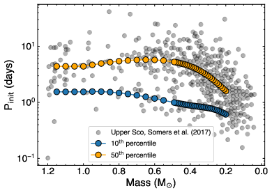
Figure 1: The Upper Sco rotation distribution at 10 Myr (Somers et al., 2017) from which we adopt the initial rotation periods for the model tracks. The solid blue and yellow lines show a 1-D smoothing spline fit to the 10^th and 50^th period percentiles in each mass bin, respectively.

2.1.2 Magnetic braking

We adopt the van Saders & Pinsonneault (2013) formulation of the classic wind braking law proposed by Kawaler (1988)

$$\frac{dJ}{dt}=\left\{\begin{array}[]{ll}f_{K}K_{M}\omega\left(\frac{\omega_{\mathrm{sat}}}{\omega_{\odot}}\right)^{2}&\omega_{\mathrm{sat}}\leqslant\omega\frac{\tau_{cz}}{\tau_{cz,\odot}}\\ f_{K}K_{M}\omega\left(\frac{\omega\tau_{cz}}{\omega_{\odot}\tau_{cz,\odot}}\right)^{2}&\omega_{\mathrm{sat}}>\omega\frac{\tau_{cz}}{\tau_{cz,\odot}}\end{array},\right.$$ (1)

where $f_{K}$ is a normalization constant tuned to reproduce the observed rotation at known age; $\omega$ is the rotation rate; $\omega_{\odot}$ is the rotation rate of the Sun ($2.86\times 10^{-6}\,\mathrm{rad\,s}^{-1}$); $\omega_{\mathrm{sat}}$ is the saturation threshold; $\tau_{cz}$ is the convective overturn timescale; $K_{M}$ is the product

with luminosity $L$, mass $M$, radius $R$, photospheric pressure $P_{\mathrm{ph}}$; $c(\omega)$ is the centrifugal correction from Matt et al. (2012). As in van Saders & Pinsonneault (2013), we assume that the magnetic field scales as

$$\frac{\dot{B}}{\dot{B_{\odot}}}=\left(\frac{P_{\mathrm{phot}}}{{P_{\mathrm{phot},\odot}}}\right)^{0.5}\left\{\begin{array}[]{ll}\frac{\omega_{sat}}{\omega_{\odot}}&\omega_{\mathrm{sat}}\leqslant\omega\frac{\tau_{cz}}{\tau_{cz,\odot}}\\ \frac{\omega\tau_{cz}}{\omega_{\odot}\tau_{cz,\odot}}&\omega_{\mathrm{sat}}>\omega\frac{\tau_{cz}}{\tau_{cz,\odot}}\end{array},\right.$$ (3)

and tie the mass loss rate to the empirical scaling of $\dot{M}$ with X-ray luminosity from Wood et al. (2005), with X-ray luminosity given by the Pizzolato et al. (2003) scaling with Rossby number ($\mathrm{Ro}=P_{\mathrm{rot}}/\tau_{cz}$)

$$\frac{\dot{M}}{\dot{M_{\odot}}}=\left(\frac{L_{bol}}{L_{bol,\odot}}\right)\left\{\begin{array}[]{ll}\left(\frac{\omega_{sat}}{\omega_{\odot}}\right)^{2}&\omega_{\mathrm{sat}}\leqslant\omega\frac{\tau_{cz}}{\tau_{cz,\odot}}\\ \left(\frac{\omega\tau_{cz}}{\omega_{\odot}\tau_{cz,\odot}}\right)^{2}&\omega_{\mathrm{sat}}>\omega\frac{\tau_{cz}}{\tau_{cz,\odot}}\end{array},\right.$$ (4)

We do not include weakened magnetic braking (van Saders et al., 2016) as the low-mass stars in our sample are not expected to reach the relevant Ro within the age of the galactic disk (van Saders et al., 2019).

2.2 AM Redistribution

For the internal AM transport, we adopt the prescription for core-envelope coupling as described in Denissenkov et al. (2010). The basic assumption of this model, which was originally proposed by MacGregor & Brenner (1991) as the double-zone model, is that the core and the envelope rotate rigidly but not necessarily at the same rate. This assumption is roughly consistent with the current rotational state of the solar interior (Denissenkov et al., 2010). The rate at which the two zones are allowed to exchange angular momentum is defined by the core-envelope coupling timescale $\tau_{c}$, which is assumed to be constant along the evolution and a function of stellar mass as in Spada & Lanzafame (2020)

$$\tau_{c}=\tau_{c,\odot}\left(\frac{M_{*}}{M_{\odot}}\right)^{-\alpha}$$ (5)

where $\tau_{c,\odot}$ is the solar rotational coupling timescale ($\approx 22$ Myr, Spada & Lanzafame 2020) and $\alpha$ is a power-law exponent of this mass-dependent timescale for transport. This scaling was found to remain consistent regardless of the choice of wind braking law and in good agreement with the separate analysis of core-envelope re-coupling by Somers & Pinsonneault (2016). Lanzafame & Spada (2015) found $\alpha=7.28$ and Spada & Lanzafame (2020) refined this estimate to $\alpha=5.6$ using new data of the clusters Praesepe and NGC 6811 that extended to lower mass stars. More recently, Cao et al. (2023) found $\alpha=11.8$ by using spotted models to fit the rotational sequences in the Pleiades and Praesepe. We leave it as a free parameter in our calibration fits.

Thus, our model has six parameters, of which three are set as follows: $P_{\mathrm{init}}$ is given by the Upper Sco rotational distribution shown in Fig. 1; the disk-locking timescale $\tau_{\mathrm{disk}}$ is set to the age of Upper Sco, 10 Myr; the solar rotational coupling timescale is fixed at 22 Myr. We fit for the remaining three parameters: the normalization constant $f_{K}$ and the saturation threshold $\omega_{\mathrm{sat}}$ in the braking law, and the exponent $\alpha$ in the core-envelope coupling timescale mass dependence.

To constrain $f_{K}$, $\omega_{\mathrm{sat}}$ and $\alpha$, we calibrate the models such that they can reproduce the rotational distributions in the Pleiades, Praesepe, M67 and the rotation period of the Sun at solar age.

2.2.1 Model Calibration

We split the cluster data into temperature bins with an equal number of points; for each temperature bin, we divide the observed rotation periods into two percentile groups, the 0-20^th and the 20-80^th groups. We initialize non-spotted ($f_{\mathrm{spot}}=0\%$) tracks with masses between 0.18 $M_{\odot}$ and 0.6 $M_{\odot}$ with a 0.01 $M_{\odot}$ step and between 0.6 $M_{\odot}$ and 1.15 $M_{\odot}$ with a 0.5 $M_{\odot}$ step. We match the tracks metallicity to that of the clusters: solar metallicity tracks are used for the Pleiades and M67; $[\mathrm{Fe/H}]=+0.2$ tracks are used for Praesepe.

We evolve each track using values of $P_{\mathrm{init}}$ drawn from a 1-D smoothing spline fit to the 10^th and 50^th percentiles in Upper Sco (Fig. 1) at the stellar mass of the track and assume that the fast rotators behave as solid body rotators (Denissenkov et al., 2010; Somers & Pinsonneault, 2016), while median rotators are allowed to undergo core-envelope decoupling. Furthermore, we treat fully convective stars as rigid rotators, since their core is no longer distinct. For each $P_{\mathrm{init}}$ percentile, we separately interpolate $T_{\mathrm{eff}}$ and $P_{\mathrm{rot}}$ as a function of age and evaluate them at the age of the clusters. We obtain a gyrochrone by further interpolating $P_{\mathrm{rot}}$ and $T_{\mathrm{eff}}$ across the full stellar mass range.

We quantify agreement between the model and observed $P_{\mathrm{rot}}$ by computing the $\chi^{2}=\Sigma(P_{\mathrm{obs}}-P_{\mathrm{mod}})^{2}/\sigma^{2}_{P}$, where $\sigma_{P}$ is the error on $P_{\mathrm{obs}}$ and is assumed to be 10% of $P_{\mathrm{obs}}$ (Epstein & Pinsonneault, 2014). Since the models are also calibrated to reproduce the solar rotation period ($P_{\odot}=25.4$ days, Denissenkov et al. 2010) at solar age ($t_{\odot}=4.57$ Gyr, Bahcall et al. 1995), we normalize the $\chi^{2}$ computed for each temperature-period percentile group in a cluster by the number of data points in the group such that each cluster’s $\chi^{2}$ has an equal contribution to the total $\chi_{\mathrm{tot}}^{2}=\chi_{\mathrm{Pleiades}}^{2}+\chi_{\mathrm{Praesepe}}^{2}+\chi_{\mathrm{M67}}^{2}+\chi_{\odot}^{2}$.

Thus, the fit includes 405 data points and three free parameters, $f_{k},\,\omega_{\mathrm{sat}},\,\alpha$. The best-fitting values of the parameters ($f_{K}=6.81$, $\omega_{\mathrm{sat}}=3.90\times 10^{-5}$ and $\alpha=10.97$; $\chi^{2}_{\mathrm{tot}}=158$) are obtained by minimizing $\chi^{2}_{\mathrm{tot}}$ through the differential evolution (DE) function from the Python library yabox (Mier, 2017). The calibrated gyrochrones evaluated at the clusters ages are shown in Fig. 2.

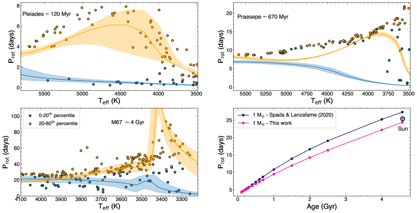
Figure 2: Two sets of gyrochrones launched from the Upper Sco rotation distribution, corresponding to the 10^th and 50^th percentiles (colored blue and orange, respectively) are shown in each plot against observed cluster member rotational sequences. These gyrochrones are fitted to the cluster’s observed periods according to matching bins (0-20^th percentiles in blue, 20-80^th percentiles in orange). Shaded regions around each gyrochrone account for the uncertainty in the cluster’s age at which the models are being evaluated. The bottom right panel shows the rotational evolution of the Sun up to its current age (indicated as a black marker) as predicted by our model and the Spada & Lanzafame (2020) model.

2.3 White Dwarf Cosmochronology

White dwarfs are the final evolutionary stage of stars with initial masses of less than roughly 8-10 $M_{\odot}$. Because they no longer undergo nuclear fusion in their cores, their evolution consists of a cooling phase dominated by the leaking of residual thermal heat from the non-degenerate ions in the electron-degenerate core. The key idea behind using WDs as cosmochronometers is that their effective temperature and mass map uniquely onto a single cooling age. The effective temperature and surface gravity of the WD, which yields its mass, can be derived from either spectroscopy or photometry coupled with model atmospheres. Once the cooling age has been determined using the WD atmospheric parameters, the next step is to estimate its progenitor MS and post-MS lifetimes. This is done by using IFMRs (e.g., Cummings et al. 2018) to correlate the final WD mass to initial ZAMS masses, from which the progenitor lifetimes are estimated. The total age of the WD is given by the sum of the cooling age and progenitor MS and post-MS lifetimes.

Due to the lack of spectroscopic observations for all the WDs in the sample, we use spectral energy distribution (SED) fitting of the mean fluxes in different bands from all-sky surveys including Gaia, the Sloan Digital Sky Survey (SDSS), the Panoramic Survey Telescope and Rapid Response System (PanSTARRS) and the SkyMapper Southern Survey. We compute total ages of the WDs following the methods outlined in Heintz et al. (2022), which we summarize below for completeness.

2.3.1 Fitting Routine

We convert model DA white dwarf spectra, spanning effective temperatures of 3000 K to $40{,}000$ K and surface gravities of 6.25 to 9.5 dex, from Koester (2010) to synthetic fluxes by using the sensitivity of each band-pass and the appropriate AB magnitude zeropoints. The assumption that all WDs are DAs can introduce systematic mass errors of $10-15$% (Giammichele et al., 2012) however, due to the lack of spectral information for the majority of the WDs, this is the simplest assumption that we can adopt. The observed magnitudes are also converted to absolute fluxes at 10 pc using AB zeropoints and the weighted mean parallax of the binary from Gaia. For SDSS $u$ and $z$, the magnitudes are shifted $0.04$ and $0.02$ mag, respectively, to account for the shift relative to the AB mag system (Eisenstein et al., 2006). The weighted mean parallax of the binary system is dominated by the brighter MS star and is on average six times more precise than the individual WD parallax which in turn allows for a more precise age determination. The observed fluxes are de-reddened using extinction values from Gentile Fusillo et al. (2021), which are obtained using the 3D extinction maps from Lallement et al. (2022). These observed de-reddened fluxes are related to the model synthetic fluxes through the radius of the WD through the following relation

$$F_{X}=\frac{R^{2}}{(3.08568\times 10^{19}\mathrm{cm})^{2}}F_{X,\mathrm{mod}}(\mathrm{T_{eff},log\ g})$$ (6)

where $F_{X}$ is the observed flux at 10 pc in bandpass $X$, $R$ is the radius of the WD in cm, and $F_{X,mod}$ is the synthetic flux in bandpass $X$ that is a function of effective temperature and surface gravity.

We use a Markov Chain Monte Carlo approach and make use of the python package emcee (Foreman-Mackey et al., 2013) to get best-fit temperatures and radii, which are represented by the 50^th percentiles of the MCMC posterior distributions. These are converted to surface gravities, masses, and cooling ages using the cooling models from Bédard et al. (2020), which assume that the WD inherits a “thick” hydrogen layer from its progenitor and thus retains its DA spectral type throughout its life. We use flat priors for the temperatures and surface gravities that cover the full range of the models. A lower limit on the magnitude uncertainties of 0.03 mag is set to account for systematics in the conversion of magnitudes to average fluxes. We also impose a lower limit on the uncertainty on the surface gravities of 0.03 dex and a lower uncertainty of 1.2% on the effective temperatures to account for any unknown systematics in the models (e.g., Liebert et al. 2005).

2.3.2 Photometric Cleaning

There is often a large luminosity contrast between the WD and the MS star in the binary, therefore an added measure of cleaning of the photometry is needed to obtain reliable parameters. We first remove photometry that is flagged for several issues in SDSS, PanSTARRS, and SkyMapper. We remove photometry from SDSS with EDGE, PEAKCENTER, SATUR, and NOTCHECKED flags. We only use photometry from PanSTARRS with rank detections of 0 or 1. We also remove any photometry from SkyMapper that has any raised flags.

Going beyond our method in Heintz et al. (2022), we also systematically remove photometry that is not consistent with the Gaia fluxes. To do this, we run the fitting routine described in Section 2.3.1. Then, we fit a line to the residuals of the resulting SED fit to account for an incorrect temperature estimate. We compare the residuals of this linear fit to the largest absolute percent deviation between Gaia $\mathrm{G,G_{BP},\ and\ G_{RP}}$. Any photometric bands that are more than $3\sigma$ away from this absolute percent deviation are removed, where $\sigma$ is the uncertainty for the individual photometric band. A new linear fit to the SED residuals is performed with these bands removed. Then, a new comparison to the largest absolute percent deviation of the Gaia bands is performed, including the previously removed bands. This iterative process continues until a consistent list of photometric bands are removed, and a final SED fit is performed. SDSS $u$-band is not subjected to this stage of photometric cleaning since it can be a strong indicator of whether the WD is a DA or non-DA due to the presence of the Balmer jump in DA WDs. The larger residual of SDSS $u$ can be indicative of a non-DA and not because the photometry is suspect (e.g. Bergeron et al. 2019). We find that $~{}30$ WDs show anomalously discrepant SDSS $u$-band photometry that suggests there may be some non-DA in the sample. However, since $>65$% of WDs in the Gaia magnitude-limited samples are DAs (Kleinman et al., 2013), adopting a DA model is a reasonable assumption.

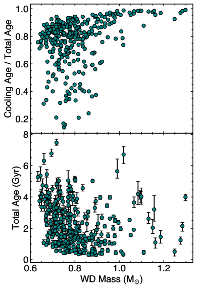
Figure 3: Top: Contribution of the cooling age to the total age of the WD as a function of mass. Bottom: WD total age as a function of mass; the uncertainties on the WD ages have been inflated by empirically determined factors (Heintz et al., 2022) to compensate for systematics on the total ages.

Moreover, Heintz et al. (2022) found that, when assuming DA spectral types for all the WD in their sample, the ages are good to 25% and provided error inflation factors to account for inaccuracies in the WD ages, including the assumption of an incorrect spectral type.

2.3.3 Progenitor Lifetimes

To get the progenitor lifetimes of the WDs, we use an IFMR from Heintz et al. (2022) which uses a theoretically motivated shape to the IFMR from Fields et al. (2016), fit to WDs in solar metallicity clusters (Cummings et al., 2015, 2016), in conjunction with the stellar evolutionary tracks from Modules for Experiments in Stellar Astrophysics (MESA, Paxton et al. 2011, Paxton et al. 2013, Paxton et al. 2015). The errors on these values are determined by using the $1\sigma$ uncertainties on the WD mass to determine an upper and lower MS mass. The difference between the central value and the upper and lower MS mass are quoted as upper and lower errors, respectively. The same process is carried out for the progenitor lifetimes as well.

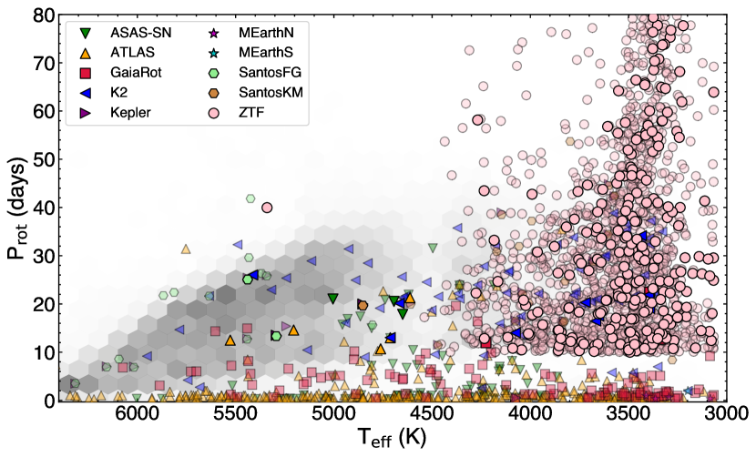
Figure 4: MS stars in the full wide WD+MS sample in a T${}_{\mathrm{eff}}-$P_rot space. 1985 rotation periods are retrieved from ZTF; 384 periods are from ATLAS; 102 periods are from Gaia DR3; K2 provides 82 periods; 78 periods are from ASAS-SN; 23 periods are retrieved from Kepler; 15 periods are from Santos et al. (2021); 20 periods are from Santos et al. (2020); 9 periods are from MEarth North and 3 periods are from MEarth South. The most opaque markers represent the MS stars in the WD + MS binaries that made it into the final selection (327 systems) described in Sec. 3. The McQuillan Kepler field (McQuillan et al., 2014a) of 34,030 MS stars below $6500\,\mathrm{K}$ is shown in the background, together with the additional detection of $15{,}640$ M and K-type Kepler stars by Santos et al. (2019).

2.3.4 Precision of Total Ages

The total age of the WDs in the sample is primarily determined by their mass, and therefore uncertainties in the WD mass have a significant impact on the accuracy of the estimated total ages. Heintz et al. (2022) found that the total ages derived from WDs with $M<0.63$ $M_{\odot}$ become very noisy. Moreover, accurately determining the ages of low-mass WDs poses a challenge due to the lack of well-defined constraints at the lower end of the IFMR. WDs with masses below $0.575$ $M_{\odot}$ may not provide reliable age estimates since they might not have formed through the evolution of a single star. While their cooling ages can offer a minimum estimate of their total age, it is essential to consider the possibility that their low mass is a result of contamination in the photometry, especially if they are formed through binary interactions.

Thus, we adopt the following: we ignore total ages obtained from WDs with $M<0.575$ $M_{\odot}$; for WDs with $M>0.575$ $M_{\odot}$, we adopt the total ages computed as the sum of the cooling age and progenitor lifetimes. To avoid contamination from the MS companion, we filter sources with a Gaia BP-RP corrected excess factor $<0.1$ (Riello et al., 2021). Because formal age uncertainties are often underestimated for higher-mass WDs, we inflate the age uncertainties by a factor computed following the comparison to wide WD+WD described in Heintz et al. (2022).

Our final sample predominantly comprises of massive WDs (with masses greater than $0.67$ $M_{\odot}$), in which the total ages are primarily influenced by cooling rather than the IFMR, as illustrated in Fig. 3. This results in an average age uncertainty of 10% prior to inflation and 20% post-inflation.

3 Sample Selection

We construct the wide binary sample using the El-Badry et al. (2021) catalog, which contains 1.3 (1.1) million binaries with a $>$ 90% ($>$ 99%) probability of being bound. Stars are classified as MS or WD based on their location on the Gaia color-absolute magnitude diagram (CMD). The absolute magnitude is defined as $M_{G}=G+5\,\mathrm{log}(\omega)-10$, where $G$ is the $G$-band mean magnitude and $\omega$ is the parallax in mas; stars with $M_{G}>3.25(G_{\mathrm{BP}}-G_{\mathrm{RP}})+9.625$ are classified as WDs; all other stars with measured $G_{\mathrm{BP}}-G_{\mathrm{RP}}$ are classified as MS stars (El-Badry & Rix, 2018). We only select systems containing a WD and an MS star and find $22{,}563$ such systems.

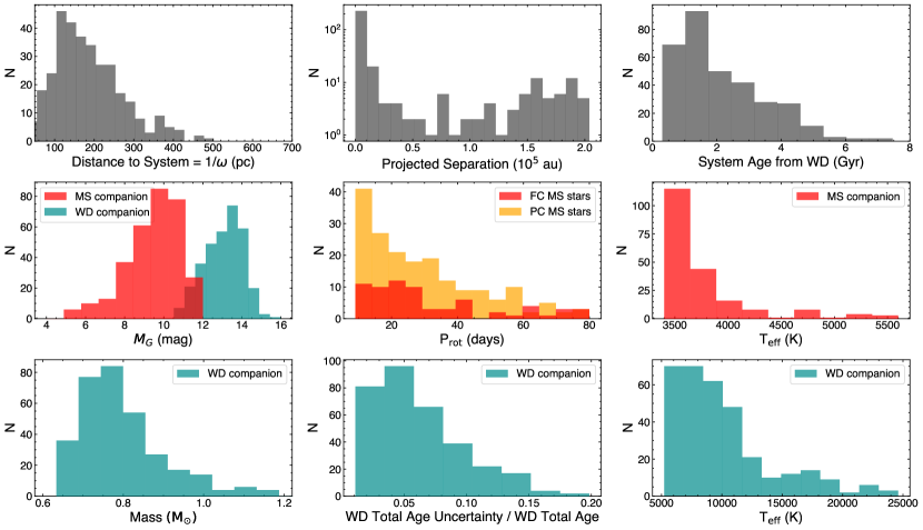
Figure 5: Properties of the 327 binaries with precise WD ages in the sample. We distinguish fully convective (FC) MS stars from partially convective (PC) MS stars based on their absolute Gaia magnitude, $M_{G}$, and Gaia BP-RP color measurements using Jao’s gap (Jao et al., 2018).

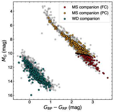
Figure 6: Gaia color-magnitude diagram showing the full data sample (2701 systems, grey markers) of WD + MS binaries for which we estimated ages from the WD companions. We highlight the 327 binaries with the most precise WD total ages (average uncertainty $<10\%$). The Jao et al. (2018) gap is shown as a solid black line.

We search for rotation periods of these MS stars in several rotation surveys, including the Asteroid Terrestrial-impact Last Alert System (ATLAS) variable stars database (Heinze et al., 2018), the All-Sky Automated Survey for SuperNovae (ASAS-SN) variable star database (Shappee et al., 2014; Jayasinghe et al., 2018), the Calar Alto high-Resolution search for M dwarfs with Exoearths with Near-infrared and optical Echelle Spectrographs (CARMENES) catalog (Díez Alonso et al., 2019), the Gaia third Data Release (DR3, Gaia Collaboration (2022)), the Hungarian-made Automated Telescope Network (HATNet) Exoplanet survey (Hartman et al., 2010), the Kilodegree Extremely Little Telescope (KELT) database (Oelkers et al., 2018), the Kepler (McQuillan et al., 2014b; Santos et al., 2020, 2021) space mission, the K2 space mission (Reinhold & Hekker, 2020), the MEarth Observatory (Newton et al., 2016, 2018) and the Zwicky Transient Facility (ZTF, Chen et al., 2020; Lu et al., 2022). We find 5005 binaries that feature an MS star with a measured rotation period, with approximately 85% of the rotation periods sourced from the ZTF catalog. Lu et al. (2022) found that nearly 50% of stars with ZTF periods $<$ 10 days are likely to be incorrect, therefore we exclude all binaries with such ZTF fast rotators. This reduces the number of WD + MS with measured rotation periods to 2701.

We cross-match these MS stars with various spectroscopic catalogs, including the Galactic Archaeology with HERMES (GALAH) survey (Buder et al., 2018), the Large Sky Area Multi-Object Fibre Spectroscopic Telescope (LAMOST) (Zhong et al., 2020), the Apache Point Observatory Galactic Evolution Experiment (APOGEE) survey (Abdurro’uf et al., 2022), and Gaia DR3 (Recio-Blanco et al., 2022). We retrieve spectroscopic properties for 430 MS stars. We use spectroscopic data when available, but do not require spectroscopy to be included in the sample.

We obtain WD ages for these 2701 binaries and select 1065 binaries with WD mass $>0.575$ $M_{\odot}$ and Gaia BP-RP excess factor $<0.1$ (see Sec. 2.3.4 for more details). Finally, we require WD ages to have the average of the uninflated low and upper uncertainties less than 20%. The final sample contains 327 binaries with precise WD ages, which we report in Table LABEL:samp in the Appendix. The distribution of rotation periods across the different catalogs used to create the sample is presented in Fig. 4. Effective temperatures of the MS stars were computed from G_BP-G_RP measurements using a polynomial fit taken from Curtis et al. (2020), assuming no extinction. Their color-temperature relation was constructed using nearby benchmark stars, including a sample of low mass stars with 3056 K $<$ $T_{\mathrm{eff}}$ $<$ 4131 K and $-0.54$ dex $<~{}\mathrm{[Fe/H]}~{}<$ +0.53 dex from Mann et al. (2015). The basic properties and CMD of the sample are shown in Fig. 5 and 6, respectively.

4 Results and Discussion

4.1 Model Assessment

In general, our gyrochrones reasonably match the rotation sequences observed in the clusters, with the exception of K-dwarfs in Praesepe. Specifically, for K-dwarfs with effective temperatures between $4250\,\mathrm{K}$ and $5000\,\mathrm{K}$, our models predict rotation periods that are a few days shorter than those observed. We note that there are no super-solar metallicity atmospheric tables available from Allard et al. (1997), therefore we have approximated the metal rich case with the solar atmosphere. However, we do not get very different best-fit parameters if we use solar metallicity tracks for all clusters, including Praesepe. At $\sim 670$ Myr, these K-dwarfs experience core-envelope decoupling. The fitted coupling timescale in this work has a strong mass dependence, therefore, these low-mass stars take an extended period before resuming their spin-down. Here we adopt a constant, rotation-rate independent coupling timescale, although we expect this timescale to change with time. We suspect that this coupling timescale prescription is contributing to the morphology mismatch between the cluster and the model, which appears to be a more significant concern than differences in atmosphere or metallicity. Exploring more nuanced prescriptions that depend on evolutionary state and rotation rate are well-motivated, but beyond the scope of this work.

The bottom right panel in Fig. 2 shows that our models predict the rotation of the Sun at solar age within $\sim 1$ day. Our models reproduce the 4 Gyr M67 cluster sequence in the cool stars Dungee et al. (2022) (Fig 2, lower left panel).

Another assessment of our models is presented in Fig. 7, where we show a set of gyrochrones against the ZTF rotation period catalog from Lu et al. (2022). The ZTF distribution shows an overdensity of fully convective stars rotating slowly ($P_{\mathrm{rot}}>40$ days) past the closing of the intermediate period gap, a period dearth in the T${}_{\mathrm{eff}}-\mathrm{P}_{\mathrm{rot}}$ space for low-mass stars that was first detected with Kepler by McQuillan et al. (2013). This increase in rotation period for such stars is also predicted by gyrochrones older than 2 Gyr. We note that while the apparent agreement with the ZTF is good, the earlier McQuillan et al. (2014a) sample contains lower amplitude, more slowly rotating stars at these temperatures that are not fit by our gyrochrones. These stars are presumably older than 4 Gyr, and suggest that our core-envelope coupling prescription may be overly simplistic. Even if this is the case, it does not fundamentally alter the conclusions of this paper.

The best-fit parameters obtained from the clusters fit are in agreement with those from Cao et al. (2023) ($f_{k}=9.79\pm 0.37$,  $\omega_{\mathrm{sat}}=(3.466\pm 0.085)\times 10^{5}\,\mathrm{rad\,s^{-1}}$ and $\alpha=11.8\pm 1.0$), who calibrated spotted models (Somers et al., 2020) to the Pleiades and Praesepe. We find a higher value of $\alpha$ compared to the value reported in Spada & Lanzafame (2020) ($\alpha\approx 5.6$), although their models did not include stellar spots (which alter the mass-temperature relation and therefore apparent mass-dependece of $\alpha$) and assumed a fixed initial rotation period of 8 days for all stellar masses rather than a distribution of $P_{init}$. Moreover, their two-zone model has been calibrated for stellar masses down to $\approx 0.4M_{\odot}$.

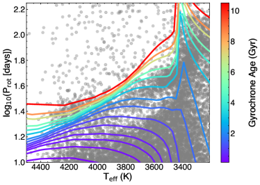
Figure 7: ZTF stars from Lu et al. (2022) are plotted as grey circles. Our gyrochrones are shown as solid lines and color-coded by their age. The gyrochrones are constructed using a non-spotted solar-metallicity grid and launched from the median $P_{\mathrm{init}}$ percentile in Upper Sco.

4.2 A spike in $P_{\mathrm{rot}}$ at the fully convective boundary

Using the best-fit parameters, we construct gyrochrones to predict the rotation period of the stars in our sample at the age inferred from their WD companions. To make a direct comparison between model and observed rotation periods, we create a grid of $f_{\mathrm{spot}}=0\%$, solar-metallicity tracks for stellar masses between 0.18 and 1.15 $M_{\odot}$. For each stellar mass, we launch a track with $P_{\mathrm{init}}$ values between the $5^{\mathrm{th}}$ and the $95^{\mathrm{th}}$ percentiles of the Upper Sco period distribution (Fig. 1). For each star in our data sample, the model rotation period $\overline{P_{w}}$ is computed as the likelihood weighted average of the rotation periods in the grid

$$\overline{P_{w}}=\frac{\sum_{i=1}^{n}\Delta t\Delta m\mathcal{L}_{i}P_{i}}{\sum_{i=1}^{n}\Delta t\Delta m\mathcal{L}_{i}},$$ (7)

where $\Delta t$ and $\Delta m$ are the time and mass increments between each point on our non-uniformly sampled model grid, respectively; $P_{i}$ is the $i^{\mathrm{th}}$ model rotation period in the grid; $\mathcal{L}_{i}$ is its corresponding likelihood. The likelihood function accounts for the uncertainty on the WD age, taken as the average of the inflated (as per Heintz et al. 2022) lower and upper uncertainties, and the effective temperature of the MS star, computed as the root sum of the squares of the typical temperature precision ($\pm 50$ K) and the uncertainty obtained from propagation of the Gaia $G_{\mathrm{BP}}-G_{\mathrm{RP}}$ uncertainties involved in the color-$T_{\mathrm{eff}}$ relation (Curtis et al., 2020). The discrepancy between the observed and model rotation periods is quantified as the difference between $P_{\mathrm{rot}}$ and $\overline{P_{w}}$, i.e. $\lvert\Delta P_{\mathrm{rot}}\rvert$, divided by the likelihood weighted standard deviation $\sigma_{w}$ of the model periods, defined as

$$\sigma_{w}=\sqrt{\frac{\sum_{\mathrm{i}=1}^{\mathrm{n}}\Delta t\Delta m\mathcal{L}_{\mathrm{i}}\left(\mathrm{P}_{\mathrm{rot}}-\overline{P_{w}}\right)^{2}}{\sum_{\mathrm{i}=1}^{\mathrm{n}}\Delta t\Delta m\mathcal{L}_{\mathrm{i}}}}$$ (8)

The lower the ratio $\lvert\Delta P_{\mathrm{rot}}/\sigma_{w}\rvert$, the smaller the discrepancy is. The results are presented in Fig. 8. 65% of the rotation periods predicted by non-spotted, solar-metallicity models are within $3\sigma_{w}$ from the observed rotation periods and fall in the region bounded by the gyrochrones computed at the lower and upper WD age bounds in each bin.

At the fully convective boundary, our sample shows a rapid increase in the rotation period of MS stars with WD ages up to 7.5 Gyr. The same trend is confirmed by the gyrochrones ([Fe/H]$=+0.0$, $f_{\mathrm{spot}}=0\%$), which span periods between 30 and 80 days across a narrow temperature range ($\sim 50$ K) for ages up to 2.5 Gyr. Similarly, between 2.5 and 5 Gyr, the models show a sharp rise in rotation period from 50 to 170 days and up to 200 days between 5 and 7.5 Gyr. Thus, both the models and data suggest that, at the fully convective boundary, stars with relatively long rotation periods are not necessarily old, in contrast to the standard picture of stellar spin-down. In addition, at this boundary, a measured rotation period cannot be uniquely associated (within reasonable observed errors in $\mathrm{T_{eff}}$ of $\simeq$50 K) to a single gyrochrone – rather, gyrochrones spanning several billions of years all provide reasonable matches to the observed ($P_{\mathrm{rot}},\,T_{\mathrm{eff}}$) combination. This significantly inflates the age uncertainties on rotation-based ages in this $T_{\mathrm{eff}}$ range as the rotation period of a star along this vertical incline is predicted, within 1$\sigma$, by gyrochrones between 2 Gyr and 8 Gyr.

Beyond the fully convective boundary, our models return to a reasonable behavior without distinct features. This suggests the feasibility of applying gyrochronology to the coolest fully convective stars, at least from a model standpoint.

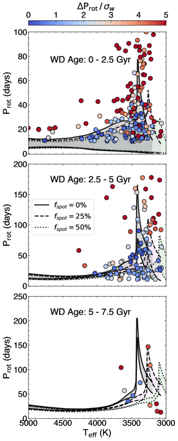
Figure 8: MS stars binned by their companion WDs ages. The grey shaded regions show the range of rotation periods spanned by $f_{\mathrm{spot}}=0$, solar-metallicity gyrochrones launched from the median percentile of Upper Sco at the WD age bounds, which are plotted as black solid line. Gyrochrones with $f_{\mathrm{spot}}=25\%$ and $f_{\mathrm{spot}}=50\%$ launched with the same $P_{\mathrm{init}}$ at the same ages are plotted as black dashed and dotted lines, respectively, and the corresponding region of allowed rotation periods is shown in light pink and green. Stars are color coded by $|\Delta P_{\mathrm{rot}}/\sigma_{w}|$ (see Sec. 4.2). Blue points show good agreement, while the redder points show worse agreement between the observed and the predicted rotation periods.

4.3 Model description of the spike

Stellar interior theory predicts that as the stellar mass decreases, the convection zone (CZ) deepens in the interior of the star until the star becomes fully convective at $\sim 0.35\,\mathrm{M}_{\odot}$. The convective overturn timescale refers to the characteristic timescale of convective motions. In this work, we compute the characteristic convective overturn timescale as the local $\tau_{cz}=H_{P}/v$, where $H_{P}$ is the pressure scale height at the base of the convective zone and $v$ is the convective velocity (from a mixing length theory of convection) one pressure scale height above the convective zone boundary. As we approach the fully convective boundary, the convective envelope gets deeper, occupying a larger part of the total stellar mass, the pressure scale height increases and the convective velocity decreases, as predicted by the mixing-length theory (Böhm-Vitense, 1958). This leads to an increase in $\tau_{cz}$.

However, it has been shown that the behavior of models near the transition to the fully convective regime is not smooth. The van Saders & Pinsonneault (2012a) instability predicts that low-mass stars at the boundary undergo non-equilibrium ³He burning, which gives rise to a small convective core separated from the convective envelope by a thin radiative zone. As the amount of central ³He increases, the convective regions grow in mass and the convective envelope deepens, until they merge, leading to a fully convective episode. This process repeats until the total ³He concentration is high enough that the star remains fully convective.

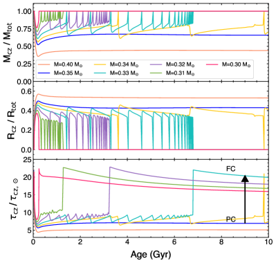
Figure 9: The sizes of the convective zone relative to the total size of the star in mass and radius coordinates as a function of time are plotted in the top and middle panels, respectively. The bottom panel shows the convective overturn timescale normalized by the solar value as a function of time. The black arrow shows the jump between partially convective (PC) and fully convective (FC) stars. In all panels, the saw-toothed curves represent stars undergoing fully convective episodes driven by non-equilibrium ³He burning (van Saders & Pinsonneault, 2012a). All tracks have solar-metallicity and a 25% spot covering fraction.

In the models used in this work, the van Saders & Pinsonneault (2012a) instability occurs for masses between 0.30 $M_{\odot}$ and 0.37 $M_{\odot}$, depending on the metallicity and spot covering fraction. For instance, in a solar-metallicity, $f_{\mathrm{spot}}=25\%$ model grid, the van Saders & Pinsonneault (2012a) instability affects models in the $0.31-0.34$ $M_{\odot}$ range and the fully convective boundary is at $0.31$ $M_{\odot}$. This is shown in Fig. 9. In the top panel, we see that as we move from a $0.4\,M_{\odot}$ partially convective star to $0.31\,M_{\odot}$, the contribution of the mass of the convective zone to the total stellar mass increases, until the star is fully convective and $M_{cz}/M_{tot}=1$. Similarly, the middle panel shows that the base of the convective zone is eating downward in mass and deepening in the interior as we approach the fully convective boundary, which makes $\tau_{\mathrm{cz}}$ longer. Furthermore, due to fully convective episodes initiated by non-equilibrium ³He burning, the convective zone base of stars in the range $0.34-0.31$ $M_{\odot}$ suddenly moves from a fractional depth $R_{cz}/R_{tot}=0.4-0.3$ to the center of the star $R_{cz}=0$, which results in discontinuous jumps in $\tau_{\mathrm{cz}}$, as seen in the bottom panel. The convective overturn timescale maxima are in phase with drops in $R_{cz}/R_{tot}$ and peaks in $M_{cz}/M_{tot}$ and correspond to fully convective episodes.

We suggest that it is the rise in $\tau_{\mathrm{cz}}$ due to differences in the structure of partially and fully convective stars that causes the vertical feature in $P_{\mathrm{rot}}$ for low-mass stars older than 1 Gyr, and that its sharpness is caused by the fact that the CZ boundary does not smoothly move towards the core (as a function of mass) until the star is fully convective, but rather jumps from a partially convective configuration in stars undergoing the van Saders & Pinsonneault (2012a) instability.

To show how $\tau_{\mathrm{cz}}$ affects stellar spin down at the fully convective boundary, we consider the relative contribution of all terms involved in the braking law. We evaluate the weight of the factors affecting $dJ/dt$ as a function of stellar mass at the median age of the data sample ($\sim 2$ Gyr). Since the majority of the stars in the sample are M dwarfs that slowly evolve on the main sequence and the structure is very stable after the fully convective episodes, the contribution of the structural terms in the braking law do not significantly depend on the age at which they are evaluated. The results are shown in Fig. 10: while the stellar mass, radius, luminosity and pressure factors vary smoothly for stars with masses between $1.15M_{\odot}$ and $0.2M_{\odot}$, the convective overturn timescale factor changes abruptly at the fully convective boundary, between $0.33M_{\odot}$ and $0.31M_{\odot}$. In this narrow mass range, $\tau_{\mathrm{cz}}$ rapidly increases as we approach $0.33\,M_{\odot}$, reaches a peak at $0.31\,M_{\odot}$, and then drops modestly. No other stellar property exhibits such a distinct feature at this boundary.

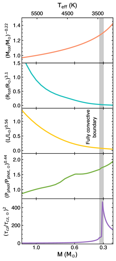
Figure 10: Contributions of the stellar mass $M$, radius $R$, luminosity $L$, photospheric pressure $P_{\mathrm{phot}}$ and convective overturn timescale $\tau_{cz}$ factors to the total $dJ/dt$ using solar-metallicity models with 25% spot covering fraction. The fully convective boundary is at $M=0.31M_{\odot}$.

The peak in the $\tau_{\mathrm{cz}}$ curve in the bottom panel of Fig. 10 is reached by the model with the largest mass — and thus largest $H_{P}$ — that becomes fully convective, which is the $0.31\,M_{\odot}$ model in the solar-metallicity, $f_{\mathrm{spot}}=25\%$ model grid. Below this point, stars are fully convective since they never have a radiative core. However, they are also smaller in radius and mass of the CZ, therefore $\tau_{\mathrm{cz}}$ drops.

4.3.1 Calibrations for $\tau_{cz}$ across the fully convective boundary

Literature sources do not agree on a single method for computing the convective overturn timescale from a stellar model, but we argue here that the sharp increase in the convective overturn timescale that drives rapid braking is a ubiquitous feature across common prescriptions for inferring the timescale.

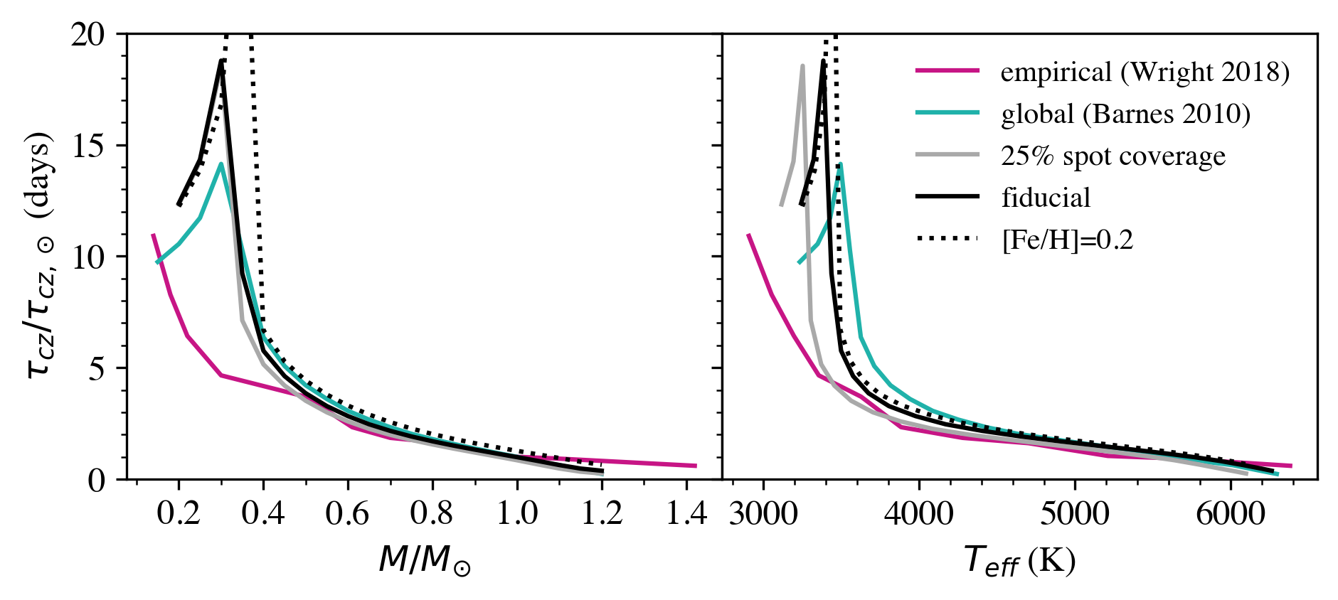
Figure 11: Comparisons of $\tau_{cz}$ values as a function of mass (left panel) and effective temperature (right panel). We show our fiducial, solar metallicity unspotted stellar models as a solid black curve. Models with identical physics but a 25% spot covering fraction are shown in gray. The Wright et al. (2018) empirical calibration is shown in purple, and the Barnes & Kim (2010) “global” model-based $\tau_{cz}$ are shown in turquoise. Metal-rich ($\textrm{[Fe/H]}=+0.2$) models are shown as the dotted curve.

When using models to compute convective overturn timescales, there are two primary approaches: the “local” prescription (used here) and a “global” prescription, where one instead computes some suitable average $\tau_{cz}$ over the entire convection zone. Both approaches yield fundamentally the same behavior modulo a scale factor, since the deep portions of the CZ probed by the local approach are also the most heavily weighted in the global average (Kim & Demarque, 1996). We show in Fig. 11 that our fiducial model, which uses a local approach, displays fundamentally the same behavior as that in Barnes & Kim (2010), which utilizes a global approach. Once normalized by their respective solar convective overturn timescales, both methods show the same behavior as a function of mass and a rapid increase in $\tau_{cz}$ near the fully convective boundary as the $\tau_{cz}$ computation begins to probe the structure of the near core.

While the location in mass (or temperature) of the sharp rise in $\tau_{cz}$ depends on properties like the metallicity and spot covering fraction, both produce only modest shifts in the precise location of the rise in $\tau_{cz}$, also shown in Fig. 11. In the case of metallicity, stars are more convective at higher metallicity but fixed mass, shifting the rise in $\tau_{cz}$ and onset of full convection to slightly higher masses in metal-rich stars, although this vertical feature does not significantly move in temperature, as shown in Fig. 12.

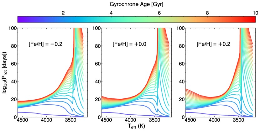
Figure 12: Gyrochrones constructed using a metal-poor (left), a solar metallicity (center) and a metal-rich (right) non-spotted model grid. We show gyrochrones for ages between 0.1 and 10 Gyr, with a step of 0.5 Gyr. While the location of the steep rise in $P_{\mathrm{rot}}$ is shifted to slightly higher masses in metal-rich stars, the feature does not vary significantly in temperature and occurs at $\approx$$3500$ K across all model grids.

Adding spots to the surface of the model — which may be an important component in modeling young, low-mass stars (Cao et al., 2023) — decreases the observed effective temperature, with only modest impacts on the structure of the deep interior (see Somers & Pinsonneault, 2015), which shifts the onset of deep convection and large $\tau_{cz}$ values to lower effective temperatures but not significantly lower stellar masses. We find that the maximum stellar mass undergoing fully convective episodes decreases with increasing spot covering fraction: 0.34 $M_{\odot}$ for 0% spot covering fraction; 0.33 $M_{\odot}$ for 25% spot covering fraction; 0.32 $M_{\odot}$ for 50% spot covering fraction. Furthermore, a higher spot covering fraction leads to a lower peak rotation period, which is a direct consequence of the onset of the ³He instability shifting to lower masses and therefore lower convective overturn timescales, as shown in Fig. 13. While the precise location of the steep rise in $\tau_{cz}$ depends on the model physics, the existence of a steep rise does not.

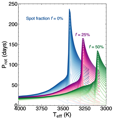
Figure 13: Solar-metallicity gyrochrones up to 10 Gyr constructed using three model grids with different spot covering fractions $f_{\mathrm{spot}}$. The sharp rise in rotation period occurs for the same 0.30-0.34 $M_{\odot}$ mass range across the three model grids, however the location of this feature varies across a $\sim$$350$ K temperature window between the three model grids with different spot-covering fractions.

Finally, attempts to develop purely empirical calibrations of $\tau_{cz}$ also predict an increase in overturn timescale across the fully convective boundary. Wright et al. (2018) made the assumption that fully convective M dwarfs obeyed the same Ro-activity relation as partially convective stars, and then found the values of $\tau_{cz}$ as a function of color (mass) that minimized scatter in the Ro$-$X-ray luminosity relation. Although the resulting relation does not trace the model predictions exactly (Fig. 11), it does indicate a reasonably steeply rising $\tau_{cz}$ across the fully convective boundary.

4.4 A Few Complications

We find that 46% of the MS stars shown in Fig. 8 have $\Delta P_{\mathrm{rot}}/\sigma_{w}>3\sigma_{w}$, i.e. their rotation rate as predicted by our spin-down model is at odds with the apparent system age given by the WD. This percentage goes down to 26% if we exclude MS stars with an effective temperature within 200 K from the fully convective boundary. We argue that these discrepancies may have multiple potential sources.

4.4.1 Stellar Spots

The model rotation periods of M dwarfs in our sample shown in Fig. 8 were obtained using a model grid with solar metallicity and $f_{\mathrm{spot}}=0\%$. However, by adopting a model grid with a non-zero spot covering fraction, we can extend the region probed by our models to cooler temperatures, as shown in Fig. 13. For instance, Fig. 8 shows that MS stars cooler than 3200 K that fall outside of the grey region bounded by the $f_{\mathrm{spot}}=0\%$ gyrochrones, are found within the region bounded by the $f_{\mathrm{spot}}=25\%$ and $f_{\mathrm{spot}}=50\%$ gyrochrones. Therefore, knowing the $f_{\mathrm{spot}}$ of these stars would be helpful to choose the most appropriate tracks to model their spin-down and improve the comparison between the predicted and observed rotation periods.

4.4.2 Metallicity

Metallicity may also be responsible for some of the discrepancies observed in our data. In the absence of spectroscopic data, we have assumed a solar-metallicity for our sample. Modern braking laws, including the van Saders & Pinsonneault (2013) prescription used in this work, suggest that metallicity can have a strong impact on the rotational evolution of low-mass stars (Claytor et al., 2020; Amard & Matt, 2020). The convective overturn timescale is a direct consequence of the stellar structure and therefore is affected by the chemical composition of the star. Stars with a high abundance of elements heavier than He have a higher opacity, which steepens radiative temperature gradients, leading to deeper convective envelopes (van Saders & Pinsonneault, 2012a; Amard et al., 2019), higher pressure scale height and, therefore, a longer $\tau_{\mathrm{cz}}$ and more efficient braking. We find that 94% of the stars with $\lvert\Delta P_{\mathrm{rot}}\rvert/\sigma_{w}>3$ have observed rotation periods that are longer than the model periods (i.e. a positive $\Delta P_{\mathrm{rot}}$). This percentage does not significantly change when not accounting for stars within 200 K from the fully convective boundary (91%).

Since higher metallicity leads to stronger braking, by adopting a metal-rich model grid we expect to recover longer model rotation period that may provide a better match to the measured rotation periods. Fig. 14 shows the difference between computing $\Delta\mathrm{P}_{\mathrm{rot}}/\sigma_{w}$ using a solar-metallicity model grid, like the one used in Fig. 8, versus a higher-metallicity model grid. By adopting an [Fe/H] = +0.2 grid, we obtain an improvement in the predictions of rotation periods for only a handful of stars with $\Delta P_{\mathrm{rot}}/\sigma_{w}>3$ when computed with a solar-metallicity grid, as shown in Fig. 14. Nevertheless, marginalizing over metallicity when constructing a model grid may improve the predictions of the rotation periods for systems with known metallicities.

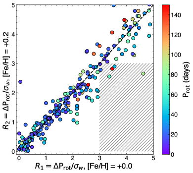
Figure 14: Comparison between $\Delta\mathrm{P}_{\mathrm{rot}}/\sigma_{w}$ computed for the MS stars in our sample using a [Fe/H] = +0.0 and a [Fe/H] = +0.2 model grids. Stars are color-coded by their observed rotation period. A 1:1 line is plotted as a black dashed line. The hatched region in the bottom right corner highlights stars for which $\Delta\mathrm{P}_{\mathrm{rot}}/\sigma_{w}$ decreases to $3\sigma_{w}$ or lower if a higher metallicity model grid is adopted instead of a solar metallicity one. Only a handful stars show improved values of $\Delta\mathrm{P}_{\mathrm{rot}}/\sigma_{w}$ when using an [Fe/H] = +0.2 model grid.

Of the full sample, only 28 MS stars have measured metallicities. We find no evident trend with metallicity in those stars where measurements are available.

4.4.3 WD Age Resets in Triple Systems

We have neglected the possibility of triple systems where the inner WD binary merges and resets the apparent system age. Modeling the evolution of single star and binary populations has shown that the age of a merger remnant can be underestimated by a factor of three to five if single star evolution is assumed for a WD (Temmink et al., 2020). The same study found that WDs from binary mergers make up about 10-30% of all observable single WDs and 30-50% of massive ($>$0.9 $M_{\odot}$) WDs. Similarly, Heintz et al. (2022) estimated that $21-36$% of WD+WD pairs likely started as a triple system. These values are consistent with the fraction of binaries in our sample ($\approx$30%) for which the models are unable to predict the rotation periods of the MS companions.

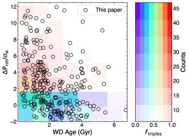
Figure 15: In the background, a 2D histogram shows the distribution of $\Delta P_{\mathrm{rot}}/\sigma_{w}$ relative to the ages of WDs in a sample drawn from a synthetic population. Each bin is color-coded based on the fraction of triples (i.e. the number of WDs in the bin that have had their age reset), while the transparency reflects the total count of WDs in the bin. Warmer colors signify a higher proportion of WDs merger products, and greater opacity indicates a larger overall WD count in the bin. The black circles represent the distribution of the observed sample. At young WDs ages, the observed sample exhibits an increased occurrence of systems with $\Delta P_{\mathrm{rot}}/\sigma_{w}>2$ in a region prone to triple contamination, as indicated by the synthetic population.

To test whether the discrepant systems in our sample may be reasonably accounted for by binary mergers, we randomly draw values of age and mass from a uniform distribution of ages up to 10 Gyr and a uniform distribution of masses between 0.18 and 1.15 $M_{\odot}$, respectively. We find the point in our model grid that is closest to each age-mass combination and construct a synthetic population of 500 MS stars with an age, mass, rotation period and effective temperature. We reset the age of 30% of the stars in this synthetic population to a number randomly drawn from a uniform distribution between 0 and the true model age to simulate an apparent age that has been reset by a merger event. From this synthetic population, we draw a sample of 400 stars that matches the observed distribution of WD ages and compute $\Delta P_{\mathrm{rot}}/\sigma_{w}$ for each star in the sample.

We find that 42% of the MS stars in our data sample have a positive $\Delta P_{\mathrm{rot}}/\sigma_{w}>3$, i.e the age that we would infer from the rotation period of the MS star is older than what we estimate from their WD companions. The synthetic population reveals that 20% of the stars have a positive $\Delta P_{\mathrm{rot}}/\sigma_{w}>3$. The 2D histogram in the background of Fig. 15 shows the distribution of $\Delta P_{\mathrm{rot}}/\sigma_{w}$ as a function of the WD age after reset in the synthetic population and highlights a tail of discrepant $\Delta P_{\mathrm{rot}}/\sigma_{w}$ values at $t<$ 3 Gyr in a region with a high fraction of triples per bin. Such a distribution is well matched by the distribution of $\Delta P_{\mathrm{rot}}/\sigma_{w}$ of our sample, as shown by the higher concentration of stars with $\Delta P_{\mathrm{rot}}/\sigma_{w}>3$ at $t<3$ Gyr and the decrease of the number of stars with $\Delta P_{\mathrm{rot}}/\sigma_{w}>3$ with age.

While we cannot identify with certainty which WDs in our sample may be the products of binary mergers, our findings suggest that a fraction of the systems showing $\Delta P_{\mathrm{rot}}/\sigma_{w}>3$ may have been triple systems that experienced merger events. Consequently, the ages we estimate for the WDs in such systems may underestimate the true system age, leading our models to predict shorter rotation periods for the companion MS stars than what is observed. We suspect, in particular, that the top panel of Fig. 8 is subject to this bias, and that some significant portion of the long period outliers may be these former triple systems.

4.5 Comparison to other datasets

4.5.1 Gyro-kinematic ages of Kepler stars

We compare the WD ages with the empirical gyro-kinematic ages from Lu et al. (2021). Gyro-kinematic ages leverage on the idea that the velocity dispersion of a stellar population at a given age increases with time due to gravitational interactions between the star and gas clouds (Spitzer & Schwarzschild, 1951). By making this assumption, Lu et al. (2021) used the rotation periods of around $30{,}000$ Kepler stars to determine their coeval nature (i.e. they assigned the same age to stars showing similar rotation periods and temperatures) and applied age-velocity-dispersion relations to estimate average stellar ages for groups of coeval stars.

We restricted our analysis to gyro-kinematic ages of stars with $3500\,\mathrm{K}<T_{\mathrm{eff}}<5000\,\mathrm{K}$, where the gyro-kinematic ages should not be impacted by weakened braking (van Saders et al., 2019). To compare this sample to our WD + MS sample, for each MS star in our sample, we created a bin centered at its $P_{\mathrm{rot}}$ and $T_{\mathrm{eff}}$ and selected gyro-kinematic stars with a $P_{\mathrm{rot}}$ and a $T_{\mathrm{eff}}$ within 5 days and 100 K from the $P_{\mathrm{rot}}$ and $T_{\mathrm{eff}}$ of the MS star, respectively. If the bin did not contain a minimum number of data points, we increased the size of the bin in the $P_{\mathrm{rot}}$ and $T_{\mathrm{eff}}$ directions by 10%; we repeated this process up to three times and until the bin contained a sufficient number of data points to obtain a median age representative of the gyro-kinematic age of the bin. We computed the gyro-kinematic age associated to the MS star in our sample as the median of the gyro-kinematic ages of the stars within the bin.

Fig. 16 shows that there is a general disagreement between WD and gyro-kinematic ages. In particular, we identify two bands in the plot: a lower band, where the age predicted by the WD companion varies between 0.1 and 4 Gyr while the gyro-kinematic age is roughly constant at 1.5 Gyr, and an upper band, where the age inferred from the WD companions is younger than the gyro-kinematic age. Our hypothesis is that the elongation in the lower band may be due to core-envelope decoupling, which would cause these stars to have a similar rotation period but different ages. WDs more accurately track the true system age, while the gyro-kinematic age is confused by groups of stars with different ages having similar rotation periods. The discrepancies in the stars populating the upper band are likely caused by a combination of two factors: 1) some fraction of the WDs in our sample are WD merger products, therefore the age inferred from the WD age is an underestimate of the true age of the system; 2) at the fully convective boundary, the gyrochrones are compressed, therefore stars at the same rotation period along this boundary are not necessarily coeval.

We find that 50% of the stars located in this upper band show a $\Delta P_{\mathrm{rot}}/\sigma_{w}>3\sigma_{w}$ and a positive $\Delta P_{\mathrm{rot}}$, which supports the WD merger hypothesis for these systems, as discussed in Section 4.4.3. Furthermore, the MS stars populating the upper band of Fig. 16 are distributed along the sharp rise in rotation period at the fully convective boundary and the disagreement between the WD and gyro-kinematic ages increases as we move toward longer periods, as shown in Fig. 17. Therefore, gyro-kinematic ages, which assume that stars at similar periods and temperatures have the same ages, are likely not reliable for stars at the fully convective boundary.

Other factors that affect the precision of WD total ages are their mass and the IFMR. Precise mass measurements and well-constrained IFMRs are required to obtain precise ages of low-mass WDs ($M<0.63\,M_{\odot}$) since their progenitor lifetimes represent a major part of their total age. However, the WD companions of the MS stars in the upper band of Fig. 17 are all high-mass WDs ($M>0.67\,M_{\odot}$), which have short ZAMS progenitor lifetimes, thus their age precision is not significantly affected by their mass and choice of IFMR. Furthermore, because formal age uncertainties of higher-mass WDs are often underestimated, we have applied inflation factors (Heintz et al., 2022). Lastly, the distribution of WD ages in our sample (grey histogram along the $x$-axis in Fig. 16) more closely resembles that of the Kepler-APOGEE Cool Dwarfs sample (Claytor et al., 2020) and Kepler field stars (Silva Aguirre et al., 2018). These age distributions peak at around 1-2 Gyr and do not exhibit the double peak observed in the gyro-kinematic age distribution (grey histogram along the $y$-axis in Fig. 16).

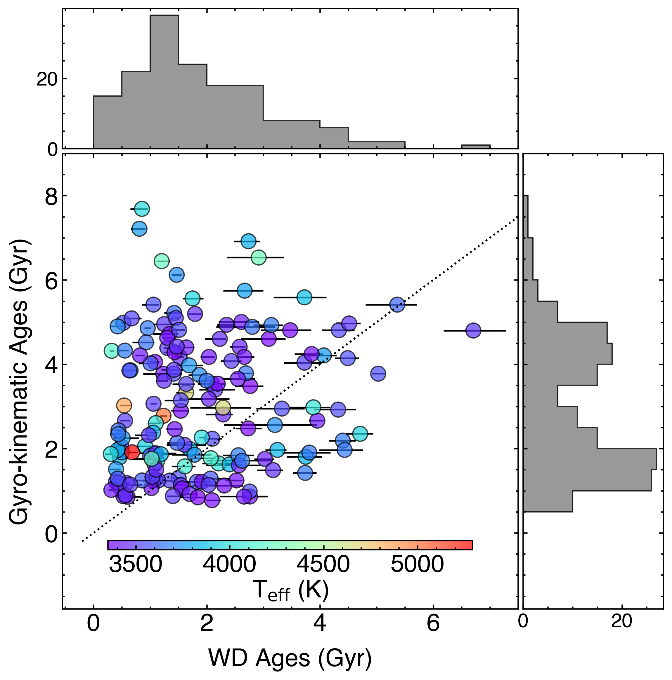
Figure 16: Comparison between the WD ages from this work and the median gyro-kinematic ages (Lu et al., 2021) computed for bins of Kepler stars around the MS stars in the sample. The data points are color-coded by the effective temperature of the MS stars. The uncertainties represent the upper and lower uncertainties on the WD ages (inflated as prescribed by Heintz et al. 2022). The histograms show the distributions of WD and gyro-kinematic ages.

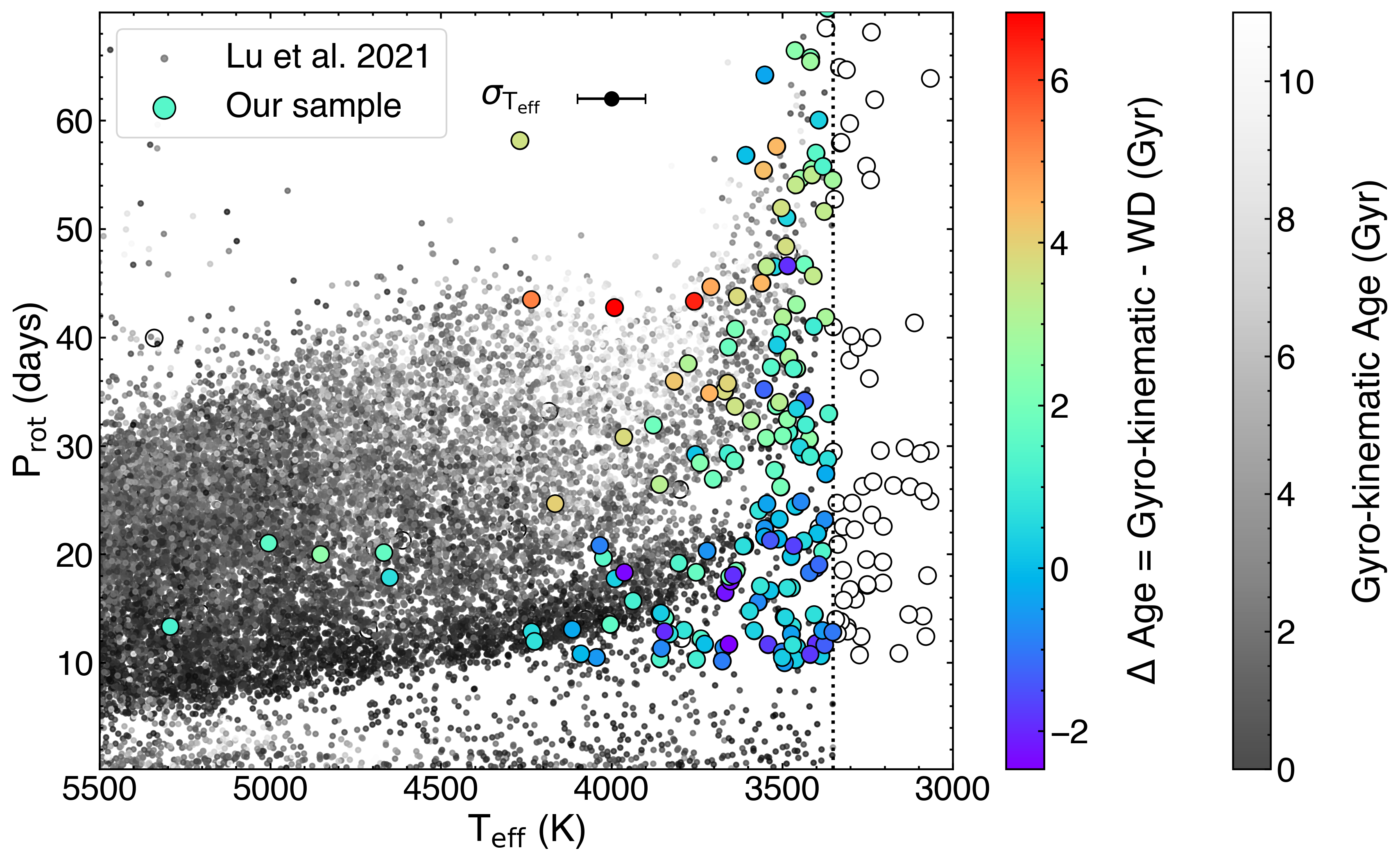
Figure 17: Kepler stars are color-coded by their gyro-kinematic ages (Lu et al., 2021) in greys. The MS stars in our sample are plotted as larger circles and color-coded by the difference between the median of the gyro-kinematic ages of the neighboring binned Kepler stars and the age inferred from the WD companions. The dashed vertical line shows the $T_{\mathrm{eff}}$ of the coolest star in the Kepler sample. Beyond this line, the cooler MS stars in our sample are plotted as white circles since there are not enough Kepler stars in the surroundings to make an age comparison. The typical uncertainty in $T_{\mathrm{eff}}$ is shown at the top.

The sharp increase of rotation periods at the fully convective boundary also challenges the hypothesis that the closing of the intermediate period gap detected in the Kepler distribution (McQuillan et al., 2013) is caused by the disappearance of the convective core, as proposed by Lu et al. (2022). We argue that perhaps it is not a lack of core-envelope decoupling, but rather the scatter of ages along the steep incline responsible for the period gap closure. Since we see a scatter of ages at the fully convective boundary, any feature that is a function of time, such as the intermediate period gap, gets “spread” across the boundary. The fact that we can have a range of ages at the fully convective boundary implies that we cannot interpret the closing of the intermediate period gap at this location as strong evidence for core-envelope decoupling, although the feature is still fundamentally tied to the loss of a radiative core.

4.5.2 Gyro-kinematic ages from Lu et al. (2023b)

The shearing flows of the solar tachocline, the transition region between the convective zone and the underlying radiative core (Schou et al., 1998), are considered to play a key role in the process of magnetic field generation. Fully convective stars do not have a tachocline and therefore are expected to have a different dynamo mechanism. Recent observations of X-ray emissions from fully convective stars reveal that these stars host a dynamo with a rotation-activity relationship that closely resembles that of solar-like stars (Wright et al., 2018), implying that the presence of the tachocline may not be a critical factor in the creation of the stellar magnetic field. However, a recent work by Lu et al. (2023b) suggested that the dynamos of partially and fully convective stars may be fundamentally different.

Using gyro-kinematic ages of a dataset that combines the Kepler stars from Lu et al. (2021) and stars with ZTF rotation periods from Lu et al. (2022) and Lu et al. (2023a), they found that fully convective stars exhibit a $\sim 2.25\times$ higher AM loss rate than partially convective stars. To account for this, they suggest that fully convective stars necessitate a dipole field strength approximately 2.5 times greater, or an approximately fourfold increase in the rate of mass loss, or a blend of both factors.

We use solar-metallicity tracks with $f_{\mathrm{spot}}=0\%$ to compute the ratio of AM loss rate of a 0.28 $M_{\odot}$ star and a 0.40 $M_{\odot}$ star at the same rotation period. We chose these masses to represent fully and partially convective stars, respectively, while also avoiding stars along the vertical feature in rotation period that we find at the fully convective boundary. For a range of rotation periods between 10 and 90 days, we find that the fully convective star always shows a higher AM loss rate than the partially convective star by at least a factor of 2, except when its rotation period is shorter than 16 days. Therefore, we suggest that invoking a modification to the stellar dynamo mechanism is not necessary to explain the stronger magnetic braking at the fully convective boundary. By scaling the torque with Rossby number, our models naturally reproduce the sharp rise in rotation period at the fully convective boundary.

4.6 Activity signatures

Because we are invoking changes in rotation period, Rossby number, and convective overturn timescales to explain the observed behavior, it is natural to ask whether there are observable activity signatures of such a physical transition.

Although the rotation periods increase across the fully-convective boundary, the convective overturn timescales also increase, meaning that we expect very modest values of the Rossby number. Stars near the “spike” in the gyrochrones achieve Rossby numbers less than solar ($\sim 2$) but greater than saturation ($\sim 0.1$) despite the extremes they represent in both rotation period and convective overturn timescale. Rotation-activity correlations have emerged from a variety of activity signatures such as X-rays (Wright et al., 2011, 2018), H$\alpha$ emission (Newton et al., 2017), UV (France et al., 2018), and show that the activity level decreases with increasing rotation period and increases with decreasing Rossby number. If magnetic activity levels truly do track Rossby number, we expect these stars to be active, but neither unusually active nor unusually quiet compared to field stars of mixed ages at slightly hotter or slightly cooler temperatures.

Stars “on the spike” do have Rossby numbers that are $\sim 0.2-0.7$ lower than stars immediately hotter or cooler than the feature, depending on the age. If we assume, for example, that magnetic activity scales as $\textrm{Ro}^{-2}$, then this corresponds to a factor of $\sim 2-20$ enhancement in activity for stars in a narrow mass range at the fully convective boundary. Observational $L_{X}/L_{bol}-\textrm{Ro}$ relations display an order of magnitude of spread in the X-ray luminosities at fixed Rossby number, making the predicted activity signature at the fully convective boundary relatively subtle in comparison. Precision activity measurements in controlled environments like open clusters may represent the best hope of detecting an activity feature at the fully convective boundary.

There have been observational efforts to examine the activity of stars in the vicinity of the fully convective boundary. Jao et al. (2023) claims that stars above the observed M dwarf luminosity gap (higher mass) are more active. In contrast, our models do not predict a lower Rossby number and higher activity rates just above the gap; instead, they predict that fully convective stars coolward (less massive) than the gap have lower Rossby numbers, and would thus appear more active (their long rotation periods are balanced by a larger $\tau_{cz}$). Because existing field samples are relatively small and challenging to control for binarity, it is not yet obvious if this apparent tension is robust.

Boudreaux et al. (2024) similarly studied the activity of gap stars, finding that there was a larger scatter in both the observed rotation rates and activity levels on the cool (lower mass) side of the gap. We create a simple stellar population where ages are drawn from a Gaussian centered on 3 Gyr with a width of 2 Gyr, truncated at 0 Gyr and 14 Gyr or the main sequence turnoff age, whichever is younger for each mass in our model grid. In this toy model the dispersion in rotation periods does indeed increase across the fully convective boundary (by about a factor of 3), as does the dispersion in predicted activity levels (again a factor $\sim 3$, assuming a $\textrm{Ro}^{-2}$ scaling for activity proxies).

5 Conclusions

In this work, we constructed a sample of 327 wide, coeval WD + MS binaries with a measured rotation period for the MS companions, which are mostly K and M dwarfs. We infer effective temperatures, surface gravities, and masses of the WD companions by using hydrogen-dominated atmosphere models and fitting photometry from a variety of all-sky surveys. Using these atmospheric parameters, we computed the total age of each WD using WD cooling models, a theoretically motivated and observationally calibrated IFMR, and stellar evolution model grids. Our sample is dominated by massive ($M>0.67\,M_{\odot}$) WDs for which the total age is primarily governed by cooling processes. This allowed us to achieve an average uncertainty of 10% on the WD total age.

To model the rotational evolution of the MS stars, we adopted an angular momentum loss prescription for magnetized winds from van Saders & Pinsonneault (2013) and modelled the internal angular momentum transport as in the standard two-zone model from Denissenkov et al. (2010). We calibrated gyrochronology models to reproduce the rotational sequences of the open clusters Pleiades, Praesepe, M67 and the rotation period of the Sun at solar age. We used the calibrated gyrochrones to predict the rotation periods of the MS stars in the sample given their effective temperature and the age from their WD companions.

We find that the rotation period steeply increases across a narrow temperature range for stars near the fully convective boundary and up to $\sim 8$ Gyr. This sharp rise in rotation period is evident in both the models and the data and suggests that stars rotating slowly at the fully convective boundary are not necessarily old.

We propose that the rise in rotation period at this boundary is driven by an increase in convective overturn timescale due to structural differences between partially and fully convective stars. As the convective envelope extends deeper into the star, encompassing a larger fraction of the overall stellar mass, it results in a rise in the pressure scale height and a reduction in convective velocity, leading to an increase in $\tau_{cz}$. Furthermore, we argue that the sharpness of such rise in $\tau_{cz}$ is induced by non-equilibrium ³He burning occurring for stars just short of the fully convective boundary (van Saders & Pinsonneault, 2012a). Although the exact location of this vertical feature in $\tau_{cz}$, and consequently $P_{\mathrm{rot}}$, depends on properties like metallicity, spot covering fraction and $\tau_{cz}$ prescriptions, the existence of this feature does not.

Due to the current uncertainties in temperature measurements, the rotation periods of stars situated along this distinct feature can be associated to a broad spectrum of gyrochrones, spanning a range of $\sim 6$ Gyr. Consequently, despite gyrochronology being regarded as a promising approach for determining the ages of low-mass stars, our findings suggest that age estimation via this method might pose greater challenges when applied to stars located at the fully convective boundary.

Future work is planned to obtain spot covering fractions for the MS stars in our sample to allow for a better comparison between the observed and the model rotation periods. Furthermore, as discussed in Sec. 4, metallicity has a non-negligible impact on stellar spin-down, therefore more robust predictions of rotation period will be achieved by taking into account the inherent variability and uncertainty associated with this parameter in our models. Having metallicity values for more stars in our sample would also allow for more accurate comparison between the observed and model rotation periods as well as better WD age estimates, since the IMFR is likely to be sensitive to the metallicity of the progenitor stars (Cummings et al., 2019). Knowing the metallicity of some of the WDs in the sample will be useful to refine the IFMRs and obtain even more precise WD ages (Raddi et al., 2022). Thus, these systems represent optimal targets for wide field spectroscopic surveys. For example, the Milky Way Mapper of the Sloan Digital Sky Survey V (Kollmeier et al., 2017) is collecting APOGEE infrared spectra for 6 million stars across the entire Milky Way and will provide metallicities for all these stars.

Having kinematic ages that remain unaffected by the rotation of main sequence stars would be advantageous. Such ages could serve as a supplementary assessment for the rapid increase in rotation period observed at the fully convective boundary. Furthermore, they have the potential to offer insights into the underlying causes of the discordance observed between the gyro-kinematic ages detailed in Lu et al. (2021) and the ages deduced from our WD sample.

Finally, our sample represents a subset drawn from a pool of 5005 WD + MS binary systems with measured rotation periods. It is worth noting that there exists a total of $22{,}563$ such systems (El-Badry et al., 2021). Access to a greater number of rotation periods would prove invaluable in expanding our sample size, probing even older age ranges, and enhancing our understanding of the rotational evolution of low-mass stars. While the count of TESS-derived rotation periods for cool, MS stars through machine learning techniques is on the rise (Claytor et al., 2023), there is also promise in forthcoming space missions like the Nancy Grace Roman Space Telescope (Spergel et al., 2015) which will enable many new rotation period measurements.

We would like to thank Dhvanil Desai, Zachary Claytor, Lyra Cao and Nicholas Saunders for helpful discussions. We acknowledge support from the National Science Foundation under Grants No. AST-1908119 and AST-1908723. JMJO acknowledges support from NASA through the NASA Hubble Fellowship grant HST-HF2-51517.001, awarded by STScI, which is operated by the Association of Universities for Research in Astronomy, Incorporated, under NASA contract NAS5-26555.

Appendix A Data Sample

Table 1: Sample of 327 MS + WD wide binaries. The reported values of $\mathrm{T_{eff}}$ and $\mathrm{P_{rot}}$ refer to the MS stars in the sample. $\sigma_{L}$ and $\sigma_{U}$ are the computed lower and upper uncertainties on the WD total age, respectively.

MS Gaia DR3 ID	WD Gaia DR3 ID	$\mathrm{T_{eff}}$ (K)	$\mathrm{P_{rot}}$ (days)	WD Total Age (Gyr)	$\sigma_{L}$ (Gyr)	$\sigma_{U}$ (Gyr)
1016412914066913792	1016427924977024768	3532	37.2	2.09	0.10	0.18
1018436324699616000	1018436320403748480	3551	22.4	1.83	0.05	0.06
1028188821038873344	1028188816743640064	3702	26.9	1.87	0.08	0.13
1033502588937866368	1033495266017587712	4165	24.7	0.32	0.02	0.02
1036217489305134848	1036217489305134976	3286	15.9	1.63	0.08	0.10
1053864376052875648	1053864371756927232	3400	11.8	2.76	0.17	0.17
1056274986577005312	1056274608619883392	3669	35.0	0.55	0.05	0.08
1059690653808481152	1059690649512906368	3551	21.6	1.50	0.04	0.05
1068143974080812160	1068340988524781952	3541	11.7	2.76	0.03	0.04
1089162891193023488	1089159966319435904	3461	24.4	1.05	0.05	0.09
1102405649756361472	1101648597344318464	3511	21.4	1.35	0.05	0.09
115344202888681216	115344095513403520	3550	64.2	4.49	0.10	0.11
1175151533777264256	1175151538072196992	3416	65.8	2.04	0.07	0.10
1202830540713288064	1202830540713287936	3372	41.8	1.09	0.04	0.05
1215379026400365568	1215379026400366080	3318	85.0	1.99	0.06	0.06
1233273646861764480	1233273646861782656	3352	77.8	1.90	0.11	0.13
1237798377728024320	1237600053318254848	3339	24.7	2.49	0.05	0.06
1246229948286292096	1246230047071154944	3534	16.7	2.10	0.08	0.07
1246239294135248512	1246239294135248384	3659	35.8	0.96	0.03	0.03
1252651160616571136	1252618213922867584	3066	63.9	4.12	0.12	0.13
1291263917336163456	1291263913040087936	3401	18.7	2.52	0.10	0.20
1322796261553157760	1322796261553165824	3787	13.0	1.06	0.05	0.11
1340289109302083584	1340289113593902080	3245	36.2	1.62	0.04	0.04
1341558083155952512	1341557984372129536	3253	55.8	2.77	0.12	0.11
1342071937339096192	1342071933043493120	3260	89.3	3.92	0.12	0.16
2187901837176956800	2187901832880159488	3480	31.3	2.15	0.17	0.13
2187942828344053888	2187942789690550272	3376	76.4	1.63	0.17	0.12
1369864498912398208	1369861200377513088	3066	128.5	1.01	0.05	0.05
2217771234476476672	2217771135693888256	3420	30.6	1.23	0.15	0.16
2221182095642372480	2221184019786046336	3413	55.5	2.61	0.14	0.18
2185748271854641024	2233787511119888000	3978	119.0	1.46	0.18	0.19
1464104190284155392	1464104190283536000	3609	20.8	0.94	0.03	0.03
2254761455631944448	2254761593070911360	3858	10.4	0.46	0.07	0.06
1481817597487494144	1481817593190278272	3422	116.8	0.97	0.05	0.06
1495234113246413440	1495233387395677952	3173	26.3	1.24	0.04	0.05
2275852459474001664	2275852455177465088	3366	28.8	2.77	0.11	0.13
2299189284536000256	2299190006090503808	3494	14.2	0.49	0.02	0.02
1557284811442449408	1557284807145814912	3243	82.9	1.09	0.05	0.08
2508478574102156544	2508478569806892928	3322	13.4	2.79	0.13	0.16
2512689428758531456	2512689424463488256	3658	29.3	2.69	0.06	0.10
1681875731024076160	1681875726730147968	3424	102.0	1.63	0.05	0.06
2539792321663876736	2539792317371533440	3310	13.3	1.46	0.10	0.20
2559242888517624320	2559255150648826112	3489	48.4	1.25	0.12	0.09
1718710573146454400	1718710568850372864	3385	84.8	1.19	0.07	0.11
2576762025758278656	2576762266276447104	4076	14.0	0.69	0.03	0.03
1766826194114207360	1766826194114406656	4612	21.3	0.77	0.03	0.03
265001616763644928	265001612467640448	3709	44.7	1.47	0.04	0.05
2656915701868610944	2656915697573351680	3458	43.0	1.52	0.04	0.04
266049206532575232	266049206532585472	3473	19.8	1.09	0.05	0.06
267776887192982784	267777604451603328	3421	29.2	3.95	0.05	0.07
268123027195914368	268123332136902016	3119	200.0	1.53	0.04	0.04
2719749527220933120	2719749527220932992	3469	102.0	0.61	0.04	0.04
2724335723363858944	2724335723364297344	3268	12.4	1.55	0.05	0.07
2736527898566892672	2736128947644568832	3078	12.4	5.14	0.08	0.09
2739560214200407168	2739560218493488512	3638	33.6	0.93	0.09	0.15
2742785532774608896	2742785322319919232	3387	88.1	0.96	0.03	0.05
1857669979411064576	1857670009471539968	3737	12.2	0.50	0.06	0.10
1874965739686844032	1874965499168713600	3858	14.5	3.25	0.08	0.10
2774575643747747968	2774583920149511040	3936	15.7	0.91	0.05	0.07
2781085405419253504	2781085401124115328	3448	159.7	3.38	0.12	0.14
2805156498090147968	2805486793959872512	3559	45.0	0.53	0.02	0.02
2824510273561942272	2824510239202203392	3364	33.0	2.20	0.08	0.11
1911106416309693952	1911106416309735552	3087	14.3	1.02	0.05	0.04
2828957042181061376	2828959305628252672	4283	170.1	0.88	0.05	0.05
2837635727977879168	2837615520155969792	3330	57.9	3.30	0.12	0.15
2840176317097371008	2840368456753528704	3546	30.7	1.42	0.07	0.08
2857544378863193472	2857547329505058176	3297	159.0	3.94	0.15	0.17
286958004978753536	287038990881256448	3303	170.1	0.60	0.06	0.06
292660381515098880	292656528929179008	3640	28.6	2.00	0.06	0.09
296479462139576576	296425242472999808	3417	65.4	1.64	0.09	0.18
2065535813733429888	2065535916813680256	3498	41.9	1.30	0.03	0.03
3063799218201750272	3063800661311469312	4761	10.7	2.15	0.15	0.10
208556331928147840	208541312424592896	3516	57.6	0.67	0.08	0.07
3094667942729601408	3094662853191563392	3718	89.0	0.35	0.06	0.03
3096007732007670144	3096007762070816128	3843	14.1	0.43	0.05	0.06
3137340435682881920	3137340435679753728	3752	18.3	0.52	0.13	0.08
3143591601666495360	3143596966081381120	3386	10.6	0.60	0.11	0.09
3145894292546764544	3145894288249489152	3375	23.2	1.92	0.10	0.19
3160143344767586176	3160143344767585536	3204	22.6	1.92	0.13	0.10
3163784102643971328	3163784441944402176	4003	13.5	0.31	0.05	0.05
3165392310198209664	3165392305902629504	3407	106.7	2.62	0.03	0.04
3266435259830726016	3266393448324042752	3295	24.7	4.56	0.09	0.11
3276414466021403008	3276414466021403264	3186	111.1	3.06	0.05	0.05
3283182338046329472	3283182265031074560	3206	17.4	1.50	0.14	0.10
3290811230756139008	3290811226460959360	3522	46.5	4.33	0.17	0.19
2238010155466716544	2238010185526881792	3372	27.4	2.73	0.16	0.15
3317635947223274752	3317636703137518208	3315	125.4	3.99	0.10	0.08
3330006857484987008	3330030565704492800	3069	138.5	0.64	0.08	0.07
3361149463489086720	3361149527909420928	3350	41.0	2.13	0.05	0.06
3369278874508583424	3369278767129521792	3667	16.5	4.40	0.14	0.14
3380358618818995328	3380357205774532480	3754	29.2	4.07	0.11	0.14
3387417517828617088	3387417513531897984	3377	51.6	1.34	0.09	0.17
340111386361933056	340111420721666048	3554	55.4	1.06	0.09	0.20
3423222461152705536	3423222559935120000	3990	17.7	1.91	0.02	0.02
3457932320957284992	3457949260309952512	3508	23.2	1.14	0.07	0.14
348345663302119936	348345659004467840	3213	144.9	3.27	0.16	0.17
3604099511263969408	3508014250968880256	3651	17.5	3.74	0.09	0.10
3610422562117192192	3610422798340344704	3434	34.2	3.03	0.09	0.11
3630646463602449664	3630648387747801088	3396	21.9	1.02	0.01	0.02
3724362340763265536	3724362336470991488	3067	24.9	1.91	0.05	0.05
3726944921778222080	3726944951843168768	3457	37.1	1.25	0.07	0.13
3727701042180797952	3727701007821059072	3237	40.0	1.64	0.05	0.06
3733304978070296320	3733305179932909312	3094	173.7	4.73	0.11	0.11
2434159727027561728	2434159727027564032	4666	20.2	1.64	0.08	0.13
374254624016996352	374254619721557504	4233	12.8	1.12	0.03	0.05
2519281859960487424	2519281855665451008	3288	75.3	3.16	0.11	0.14
3831257784633494016	3831257823288140544	3302	37.9	1.42	0.03	0.03
2567879174396642944	2567879174396643072	3437	29.2	0.58	0.04	0.05
2618616409043165824	2618616409043298688	5004	21.0	1.24	0.03	0.03
3870805121940366720	3870804537824812800	3458	129.3	1.22	0.09	0.17
3897698321657960832	3897698317362400384	3568	24.0	1.00	0.03	0.05
390689402277884544	390689397980291072	3520	89.1	2.94	0.13	0.13
3907936385524737792	3907943330487532928	3126	26.2	3.96	0.05	0.06
3912311376651443968	3912311376651444224	3221	77.7	1.30	0.04	0.03
3931756484602030976	3931756484602030848	3290	100.1	2.40	0.05	0.06
3941959093514800128	3941964964734084864	3855	14.6	1.70	0.03	0.04
3944167939359417088	3944167939360964480	3582	13.0	0.86	0.07	0.08
395377200164554368	395377513698597888	3130	14.5	5.09	0.07	0.08
3956995877097644416	3956995666643307008	4235	43.5	1.20	0.07	0.04
2743171942392459008	2743171938097183616	3470	13.3	0.45	0.07	0.06
3995728682445851648	3995728953028752768	3233	108.7	5.03	0.13	0.13
4016142868162417792	4016142868162408576	3333	87.3	2.65	0.07	0.07
411948871922982528	411951822555835648	3570	15.6	2.07	0.17	0.13
2806310641702070016	2806310603047483904	3589	84.5	0.83	0.05	0.07
2816359731303136384	2816359727009816960	3141	29.8	7.46	0.10	0.15
2828203292601777536	2828203288307357952	3333	157.9	1.25	0.02	0.03
424458153152543616	424459076562158464	3804	19.1	3.02	0.11	0.13
427169926782173056	427169583175190144	3740	28.4	1.69	0.12	0.11
2836648190441772160	2836648190441773056	3542	90.6	1.16	0.02	0.03
4283721804641828480	4283721800317089920	3319	138.5	3.75	0.07	0.09
4310991582806231296	4310991685885480064	3329	126.7	1.57	0.08	0.13
2858833212649253504	2858833208354052096	3486	51.0	4.52	0.15	0.18
434845926690890496	434857952593321088	4276	22.3	1.20	0.03	0.03
2867316941290457856	2867316975650195968	4023	19.7	1.10	0.05	0.09
2874159648826704896	2874159644531724288	3457	11.4	0.53	0.04	0.04
3074742111972735488	3074742107676979584	3498	30.9	0.56	0.04	0.05
4419026537287781632	4418831438398101376	3788	193.7	0.54	0.03	0.04
4424520144057157248	4424527561464289664	3962	18.3	4.71	0.12	0.13
4447660805076826880	4447663760014329344	3351	54.5	1.43	0.07	0.09
3129688040911585152	3129692434664991104	3277	39.1	2.37	0.05	0.06
4532268744537179904	4532250327717123968	3317	73.8	1.62	0.10	0.18
4563562151123622656	4563562426001533696	3446	54.6	2.35	0.09	0.11
4565593739374133504	4565593735079515904	3215	178.0	4.06	0.15	0.16
4590962805523660672	4590962766864961024	3373	190.7	1.92	0.06	0.06
4603527229834516096	4603528020108454528	3308	12.9	1.09	0.06	0.08
470826482637310080	470826482637310848	3233	87.1	2.63	0.03	0.03
508627314444951680	508627344501773952	3595	14.8	1.08	0.04	0.04
544555471783803136	544555467486553984	4044	10.5	2.21	0.17	0.16
564321564114510080	564509271364217344	3417	93.2	1.85	0.09	0.08
584616487177143424	584616482882438400	4112	134.5	0.53	0.03	0.05
594439627139102720	594439519764767232	4713	13.0	0.44	0.04	0.04
615513794709603200	621567804516385792	3590	32.3	1.01	0.09	0.16
6222883046075139968	6222882251504782720	3262	274.2	0.61	0.02	0.01
3839256319408219008	3839256319408293248	5527	12.5	1.94	0.10	0.18
634350314384284032	634367395469443840	3237	23.6	3.44	0.05	0.06
642718770397533568	642715055250964608	3332	64.9	0.35	0.04	0.05
642837139695905024	642837135401004672	3434	46.7	2.58	0.10	0.18
666745023612674816	666640707447423616	3553	35.2	5.03	0.06	0.05
3907622513610306432	3907622479250567808	3401	57.0	2.66	0.12	0.10
3919287679146000640	3919287674850641792	5204	14.6	1.12	0.03	0.06
678153006506212480	678153006506212608	3374	79.4	0.60	0.04	0.06
3941164971241835776	3941164966946431360	3631	43.8	1.43	0.07	0.10
70802299655353344	70802226637418496	3329	13.8	1.24	0.07	0.09
714403252037918464	714403247741604992	3853	11.3	2.40	0.11	0.10
4024591309351630848	4024591305056699136	3241	54.5	3.02	0.16	0.16
719440149164429824	719439423313644672	3375	11.6	2.09	0.08	0.06
720018767158643072	720018767158642944	3757	43.3	0.81	0.05	0.08
739321307963291136	739321312258441216	3300	16.8	1.35	0.08	0.05
748521441443836288	748521544523051136	3229	61.9	0.95	0.08	0.16
750669371768362752	750669367473333760	3412	109.1	3.00	0.16	0.15
779970154057928320	779970154057955840	3539	110.5	2.44	0.11	0.15
793941132918315392	793917660919464960	3801	26.0	1.68	0.06	0.06
794265282689661056	794265278392449664	3500	11.0	2.03	0.05	0.06
821363846267866368	821363807610959104	3347	52.7	3.03	0.12	0.15
847233808680375424	847233804386021248	3473	12.6	1.54	0.06	0.09
85649623637225856	85649413183595392	3112	41.4	3.70	0.14	0.19
4413351854700039168	4413351919121477632	3859	26.4	0.66	0.06	0.08
4434749725365419648	4434749725365419520	3440	88.2	1.03	0.02	0.02
1345042955196670208	1345041748308955648	3250	17.1	4.14	0.16	0.18
1355692412505713152	1355692408211800704	3634	18.5	0.44	0.03	0.04
1356340054918762240	1356303083840138368	3671	11.4	2.56	0.16	0.16
1357831271859374080	1357826525919678208	3381	13.0	1.56	0.04	0.04
1363780969795550336	1363761827125936128	4184	33.2	3.96	0.15	0.18
1365015515194773632	1365015545259769600	3157	93.6	3.99	0.12	0.14
4460569316402173184	4460569312107772672	3412	55.0	1.30	0.06	0.04
1397652112683641984	1397649806285796352	3750	10.3	0.40	0.04	0.06
1399620238497200896	1399620268561690240	4089	10.8	1.61	0.09	0.10
1410448641324559744	1410448259071414528	3201	130.4	1.79	0.05	0.03
1412158789927363328	1412158789927364224	3460	10.3	0.57	0.06	0.09
1428806289324715392	1428804262100101632	3473	16.9	0.40	0.08	0.05
4466814817325615360	4466814881747732480	3327	58.0	0.53	0.04	0.04
143817499599533440	143817499597885824	3288	129.2	1.84	0.08	0.13
1444622768385439232	1444622768385439104	3315	81.3	1.67	0.04	0.03
1519088739564567936	1519088735269074688	3460	54.1	1.79	0.06	0.07
1526498829461895936	1526498863822158592	3339	12.7	2.37	0.07	0.07
1541323338581798144	1541323334283923200	3163	103.6	3.12	0.13	0.13
1541905598706074880	1541905560050370816	3485	16.9	0.45	0.06	0.05
1549715047545373056	1549715047547083136	3244	88.8	0.79	0.03	0.04
4611559819405628672	4611559815111559552	3517	33.7	1.64	0.09	0.14
1588270938897733888	1588270934604149632	3964	30.8	1.75	0.09	0.08
1625475663602558208	1625661648570402304	3492	10.0	1.40	0.09	0.05
545940409758573824	545940164944375296	3502	40.4	2.44	0.11	0.11
1640003991777199872	1640200215946705024	3346	70.8	1.67	0.06	0.07
546388323308593280	546388319012071040	3253	19.5	3.85	0.18	0.20
1656963645101470336	1656967459032459520	3448	29.9	1.61	0.17	0.15
1664401914278345472	1664401914277704192	3372	68.5	2.99	0.09	0.14
166587938734739456	166587938734739328	3212	29.6	1.52	0.05	0.05
1684035206221069824	1684011837303097856	3803	19.2	1.05	0.04	0.05
865042323638265472	865042319342035328	3405	157.6	2.22	0.07	0.08
873994719110827136	873994719110827264	3322	18.6	2.36	0.06	0.06
907150801482530944	907156397824275328	3499	10.5	1.04	0.03	0.04
909162529804018688	909162525508848000	3250	17.2	1.26	0.02	0.02
936641902362276736	936641833642799744	3702	176.8	1.50	0.03	0.03
9500918630942208	9500914335389952	3425	131.0	1.10	0.05	0.06
642134100794299776	642134135154038528	3074	18.0	1.22	0.03	0.02
6527346680622426880	6527346680622426752	3392	22.5	0.48	0.05	0.06
657819944131129472	657820012850606080	3480	38.1	1.47	0.03	0.04
990883830321907456	990883830322597376	3403	120.0	1.21	0.02	0.03
991811169597579520	991811165304213760	3327	73.7	1.73	0.10	0.17
995300431092665856	995312903678079232	3865	144.7	2.54	0.03	0.04
1737075642850176000	1737075642850176128	3480	47.8	1.74	0.04	0.04
1759287667517352960	1759334156243365248	3381	20.3	1.54	0.06	0.08
1765702257007857024	1765700912683411456	3417	29.0	2.55	0.16	0.14
1791515487198244736	1791505454155264128	3469	11.6	1.10	0.16	0.13
1791860218454403968	1791857435315484032	4009	13.9	0.38	0.04	0.06
1812554680855696896	1812554676560349568	3465	292.4	0.56	0.03	0.03
1819001289330307200	1819001289323819520	3484	32.4	1.42	0.08	0.11
1822194099312577024	1822193996219126784	3302	59.7	3.26	0.15	0.16
1830600484179388416	1830600484161582464	3654	17.9	0.44	0.05	0.07
184735996626896000	184735992329821312	3409	45.7	0.82	0.06	0.06
18493721155296640	18493721155296768	3312	64.7	1.09	0.12	0.18
719562332394139776	719562332394140032	3343	14.0	0.54	0.03	0.05
741037684269171072	741037679973569408	3504	26.2	1.06	0.02	0.03
844085460212939392	844085490277157376	3713	34.8	0.43	0.05	0.06
1937074166540526976	1937827194563435648	3502	51.9	1.45	0.04	0.05
855594185859622272	855594181563866880	3508	34.0	0.63	0.03	0.03
856837802230613504	856837729215097984	3991	42.7	0.86	0.07	0.14
1969985710668480256	1969985710668477184	3252	143.5	1.96	0.05	0.06
197048465274295936	197048460976343168	3068	29.6	4.27	0.12	0.12
2010645375776770304	2010692306878145280	3406	14.4	0.32	0.04	0.02
2018812170226865664	2018818045723591680	3830	12.7	1.19	0.09	0.07
860411043221913984	860411038927355264	3614	20.8	1.48	0.07	0.10
2020837264488052864	2020837157077399552	4694	20.5	1.33	0.03	0.02
2022271027643702528	2022271027609714304	3350	29.4	1.54	0.04	0.05
2048599211506044160	2048599314570668544	3816	36.0	2.74	0.09	0.12
2053240524958351360	2053240524960871680	3407	41.0	1.43	0.08	0.11
2053585565450552960	2053584770878226304	5293	13.3	0.68	0.04	0.03
2063157913677426304	2063157260843901952	3444	24.8	1.70	0.07	0.09
2069622492291282176	2069622487994113408	3563	17.1	0.43	0.02	0.02
896972484905743872	898473932456801024	3298	40.1	1.39	0.03	0.02
2097547922975807488	2097543451912361984	3545	46.5	1.51	0.05	0.07
2099643935736477696	2099656953779008000	4852	20.0	0.54	0.06	0.04
2111700802286462848	2111335107294795520	3457	33.4	1.11	0.05	0.09
2137699338842695552	2137699712500128256	3466	37.1	0.98	0.09	0.15
2145132896436922496	2145132892139909632	3321	22.6	1.76	0.06	0.06
2157583383856242304	2157582872757579136	3490	14.2	0.65	0.10	0.08
2163324969169731072	2163324969157050112	3687	86.5	0.50	0.09	0.10
2167838052078071552	2167861618555210368	3425	153.5	3.65	0.15	0.16
1055800238072103296	1055800165056700416	3229	100.5	4.00	0.21	0.27
1214994506568260608	1214994502274335360	3483	46.6	6.71	0.26	0.24
1222565537480885376	1222565533185185024	3343	177.6	4.06	0.22	0.35
1299293685113944448	1299293680818146176	3284	76.8	3.60	0.18	0.22
1332138536976820096	1332138532682327552	3436	21.2	2.29	0.13	0.25
2272112333234818944	2224073910005362688	3184	97.9	2.01	0.11	0.21
2255996069750790528	2255996069748606976	3534	21.3	4.32	0.19	0.25
2579247712310922240	2579247708016296448	3420	18.3	2.57	0.26	0.40
2700089675200729216	2700089675200402048	3198	108.4	4.83	0.21	0.25
2709850830194329856	2709858217538113920	3656	11.7	4.44	0.17	0.23
271639471546035584	271639432884899712	3380	55.8	3.47	0.19	0.27
2745741638504666112	2745741634209187072	3775	37.6	2.67	0.23	0.27
286792799059592192	286739236524151040	3430	31.9	2.04	0.17	0.24
196589900204859392	196589861548739584	4034	20.8	3.88	0.14	0.20
293717390146554624	293717454571113984	4001	169.2	2.06	0.14	0.24
3047076750159238016	3047076750150944512	3591	270.4	5.05	0.20	0.33
3235085949939746304	3235085949939746176	3075	92.1	4.69	0.27	0.60
3238194445407460864	3238194372390557312	4268	58.1	2.92	0.22	0.28
3278241888706974336	3278241888707395584	3108	117.5	3.33	0.28	0.39
3309178916095700224	3309188669965291264	3727	11.7	1.78	0.15	0.20
3323096740440611712	3323096740438265728	3291	92.9	3.36	0.26	0.54
3389371380055187968	3389371384349749376	3095	29.3	3.03	0.22	0.50
3413008990266533376	3413009093345760768	3367	70.4	3.10	0.25	0.41
3435597013551204736	3435597013551206784	3273	10.7	2.73	0.25	0.28
3593826155650669568	3785887605544154624	3720	20.3	3.20	0.34	0.41
395932320399086464	395932247377032320	4225	12.0	1.03	0.10	0.20
4461916252508018176	4461908070590901376	4114	13.1	2.07	0.12	0.28
44769884397015296	44767955954797312	3392	19.0	2.31	0.15	0.26
4517946196857223808	4517946192529261824	4649	17.9	2.29	0.23	0.27
498275652982958848	498275652982959104	3351	12.8	1.84	0.10	0.21
506944889856368256	506944889847883008	3637	40.8	2.80	0.28	0.45
52639226555782656	52639153540042496	3877	31.9	3.73	0.20	0.28
549835601498785536	549788563014393728	3514	39.3	3.73	0.20	0.24
569795207875481344	569795203578976128	3377	72.9	5.45	0.18	0.31
583948877461123584	583949251122623232	3462	66.4	2.23	0.10	0.25
594439627139102720	594439519764767232	4713	13.0	0.44	0.04	0.04
6033508695270898432	6033508690936569344	3472	239.8	0.40	0.02	0.02
6236729088627705216	6236729329145889792	5412	26.0	6.78	0.15	0.22
3961323073827903360	3961323069532233984	3844	12.9	3.75	0.28	0.34
692919207148481920	692919202851887104	3307	130.4	4.18	0.31	0.55
748247452595214336	748247456890075136	3086	25.8	3.38	0.17	0.21
765964300065414144	765965051684223360	3392	60.0	3.85	0.20	0.30
77783305135054720	77782544925602432	3239	68.2	3.49	0.20	0.25
790463549441746944	790463545141273984	3600	112.4	2.80	0.14	0.31
4371782034475387776	4371782030179914624	3263	26.3	3.67	0.22	0.32
823582763810855168	823582759515662592	3544	24.6	3.33	0.26	0.30
851088662087300992	851088662087301120	3606	56.8	5.37	0.35	0.56
855190699452263040	855190695156439680	3204	19.3	4.28	0.18	0.23
861184515292492288	861184515291473536	3234	26.7	6.31	0.23	0.47
861951493372439424	861951489076842880	3337	20.9	2.52	0.16	0.45
4465117102652542336	4465117098356736000	3657	39.1	3.14	0.18	0.27
1604198258179547264	1604200899583092992	3400	90.4	4.75	0.24	0.42
909192835093328896	909192830801295104	3320	15.8	3.36	0.26	0.40
1748817160020646784	1748816983925915776	5340	40.0	4.06	0.20	0.27
1787683727830825856	1787683723535019776	3466	20.8	3.17	0.16	0.25
181306276262296192	181306168886213120	3675	10.2	2.63	0.31	0.36
1855910211052222592	1855910275463661440	3522	27.7	1.54	0.10	0.27
1868011126788924672	1867262393723489536	3262	146.7	5.64	0.20	0.36
192725009459729152	192701576117862400	3159	10.9	4.19	0.31	0.37
19693185261940096	19693180966870656	3469	128.4	4.00	0.28	0.47
1988383701288404992	1985376365185555200	3794	12.2	4.03	0.22	0.25
1996725077535282944	1996725077535283200	3654	104.1	5.27	0.27	0.36
2053585565450552960	2053584770878226304	5293	13.5	0.68	0.05	0.03
889041879334169344	889041668879549696	3643	18.1	3.81	0.18	0.24
2067604574919660416	2067604574919660544	3288	22.3	1.18	0.08	0.16
2080422720138489344	2080422720133121152	3779	163.1	2.60	0.23	0.28
2099643935736477696	2099656953779008000	4852	19.7	0.54	0.06	0.04
2101241457413709568	2101241281314863872	5438	25.1	2.09	0.11	0.23
2142368311889141248	2142368346248880896	3418	10.8	2.66	0.22	0.22

Appendix B Rotational Isochrones

Table 2: Rotational isochrones constructed using a solar-metallicity, $f_{\mathrm{spots}}=0\%$ model grid. Surface rotation periods are reported in days. Effective temperature are given as computed from a 2.0 Gyr gyrochrone.

$M(M_{\odot})$	$T_{\mathrm{eff}}$ (K)	Ages (Gyr)
		0.5	1.0	2.0	3.0	4.0	5.0	6.0	7.0	8.0	9.0	10.0
0.18	3200	0.48	1.13	6.36	20.15	39.02	51.46	61.47	70.09	77.79	84.83	91.35
0.19	3221	0.54	1.29	7.48	24.15	42.19	54.6	64.71	73.48	81.34	88.54	95.23
0.20	3241	0.6	1.46	8.77	27.93	45.38	57.83	68.08	77.02	85.06	92.45	99.31
0.21	3259	0.67	1.65	10.25	31.49	48.61	61.16	71.6	80.74	88.98	96.56	103.6
0.22	3276	0.74	1.86	11.95	34.96	51.95	64.67	75.32	84.68	93.13	100.91	108.14
0.23	3292	0.82	2.09	13.83	38.37	55.39	68.34	79.25	88.85	97.54	105.52	112.95
0.24	3307	0.9	2.34	16.0	41.89	59.07	72.31	83.5	93.37	102.29	110.49	118.12
0.25	3321	0.99	2.62	18.45	45.54	63.01	76.6	88.11	98.27	107.45	115.89	123.73
0.26	3335	1.09	2.92	21.2	49.43	67.33	81.33	93.2	103.68	113.14	121.84	129.91
0.27	3348	1.2	3.24	24.27	53.66	72.13	86.62	98.91	109.74	119.52	128.49	136.82
0.28	3360	1.3	3.59	27.67	58.38	77.61	92.7	105.46	116.7	126.83	136.12	144.73
0.29	3372	1.42	3.96	31.48	63.92	84.13	99.93	113.26	124.96	135.49	145.14	154.07
0.30	3383	1.54	4.35	35.71	70.69	92.19	108.86	122.86	135.11	146.1	156.15	165.45
0.31	3394	1.66	4.78	40.4	79.62	102.9	120.68	135.48	148.37	159.91	170.43	180.15
0.32	3405	1.8	5.24	45.64	93.25	119.18	138.4	154.18	167.82	179.97	191.02	201.21
0.33	3416	1.95	5.82	37.21	109.37	143.24	165.55	183.09	197.93	210.99	222.78	233.61
0.34	3426	2.16	6.53	31.0	43.21	69.29	140.69	172.77	195.51	213.87	229.62	243.6
0.35	3437	2.33	7.61	31.78	43.93	51.94	59.44	66.68	73.45	79.84	91.44	153.94
0.36	3446	1.92	4.52	19.78	32.97	43.15	51.13	57.94	64.0	68.91	73.57	78.31
0.37	3458	2.13	5.28	21.2	32.87	41.58	48.64	52.94	58.46	63.63	68.31	72.61
0.38	3470	2.36	6.18	22.09	32.71	40.01	44.45	50.4	55.81	60.57	64.94	68.85
0.39	3484	2.62	7.3	22.78	31.99	37.19	43.13	48.98	53.96	58.42	62.35	65.97
0.40	3497	2.92	8.7	23.29	30.87	36.24	42.56	47.97	52.64	56.72	60.26	63.48
0.41	3512	3.25	10.55	23.75	30.19	36.27	42.32	47.35	51.64	55.34	58.58	61.35
0.42	3526	3.65	12.1	23.81	29.86	36.12	41.82	46.46	50.34	53.63	56.45	58.79
0.43	3542	4.13	13.27	23.7	29.88	35.96	41.26	45.49	48.94	51.79	54.1	56.1
0.44	3558	4.7	14.19	23.55	29.94	35.69	40.57	44.34	47.33	49.73	51.6	53.19
0.45	3575	5.41	14.95	23.54	29.91	35.33	39.75	43.04	45.56	47.51	48.97	50.18
0.46	3592	6.27	15.57	23.66	29.79	34.88	38.73	41.51	43.56	45.09	46.26	47.08
0.47	3611	7.34	16.05	23.79	29.61	34.23	37.62	39.9	41.5	42.65	43.5	44.08
0.48	3631	8.52	16.37	23.89	29.31	33.47	36.25	38.06	39.28	40.14	40.76	41.18
0.49	3651	9.4	16.47	23.7	28.72	32.29	34.56	35.92	36.8	37.33	37.79	38.16
0.50	3673	10.12	16.71	23.77	28.28	31.3	33.12	34.14	34.8	35.26	35.56	35.89
0.51	3697	10.75	16.83	23.59	27.59	30.11	31.49	32.23	32.72	33.09	33.35	33.66
0.52	3721	11.33	17.03	23.39	26.94	28.94	29.97	30.55	30.96	31.3	31.56	31.88
0.53	3747	11.73	17.16	23.06	26.02	27.6	28.38	28.84	29.2	29.53	29.8	30.13
0.54	3774	11.99	17.16	22.43	24.86	26.08	26.65	27.04	27.39	27.73	28.06	28.35
0.55	3803	12.29	17.23	21.93	23.94	24.9	25.38	25.76	26.11	26.47	26.83	27.15
0.56	3834	12.48	17.19	21.32	22.93	23.65	24.13	24.52	24.85	25.24	25.63	26.03
0.57	3866	12.56	17.04	20.52	21.81	22.44	22.89	23.29	23.69	24.1	24.48	24.91
0.58	3900	12.65	16.8	19.73	20.77	21.35	21.81	22.24	22.68	23.12	23.53	24.01
0.59	3935	12.82	16.68	19.14	20.04	20.58	21.08	21.56	22.04	22.53	22.99	23.51
0.60	3972	12.78	16.18	18.21	18.98	19.54	20.04	20.55	21.08	21.61	22.12	22.7
0.65	4164	12.17	13.7	14.66	15.42	16.18	16.96	17.75	18.58	19.46	20.4	21.37
0.70	4395	10.35	11.09	12.2	13.34	14.55	15.84	17.23	18.7	20.23	21.85	23.6
0.75	4638	8.47	9.26	10.86	12.66	14.63	16.76	19.07	21.49	23.98	26.56	29.18
0.80	4885	7.06	8.15	10.58	13.34	16.31	19.39	22.51	25.63	28.71	31.75	34.75
0.85	5124	6.25	7.79	11.3	15.02	18.72	22.26	25.7	29.02	32.33	35.6	38.95
0.90	5347	5.79	7.89	12.34	16.58	20.5	24.18	27.76	31.3	34.9	38.66	42.72
0.95	5554	5.63	8.23	13.18	17.52	21.47	25.25	29.03	32.92	37.15	42.08	***
1.00	5742	5.58	8.46	13.46	17.73	21.67	25.55	29.66	34.37	***	***	***
1.05	5912	5.57	8.44	13.16	17.19	21.03	25.13	***	***	***	***	***
1.10	6067	5.24	7.83	12.01	15.63	19.41	***	***	***	***	***	***
1.15	6206	4.59	6.69	10.09	13.3	17.63	***	***	***	***	***	***

Notes. Models corresponding to masses greater than 0.6 $M_{\odot}$ are core-envelope decoupling models whose cores are rotating too fast, therefore the surface rotation periods reported here are an underestimate. Missing entries in a gyrochrone (indicated with ‘***’) correspond to stars that have already left the main sequence by that age and that have surpassed the critical Rossby number (Ro${}_{\mathrm{crit}}=2.08$, van Saders et al. 2019).

References

- Abdurro’uf et al. (2022) Abdurro’uf, Accetta, K., Aerts, C., et al. 2022, ApJS, 259, 35
- Adelberger et al. (2011) Adelberger, E. G., García, A., Robertson, R. G. H., et al. 2011, Reviews of Modern Physics, 83, 195
- Allard et al. (1997) Allard, F., Hauschildt, P. H., Alexander, D. R., & Starrfield, S. 1997, ARA&A, 35, 137
- Amard & Matt (2020) Amard, L., & Matt, S. P. 2020, ApJ, 889, 108
- Amard et al. (2019) Amard, L., Palacios, A., Charbonnel, C., et al. 2019, A&A, 631, A77
- Bahcall & Pinsonneault (1992) Bahcall, J. N., & Pinsonneault, M. H. 1992, Reviews of Modern Physics, 64, 885
- Bahcall et al. (1995) Bahcall, J. N., Pinsonneault, M. H., & Wasserburg, G. J. 1995, Reviews of Modern Physics, 67, 781
- Barnes (2007) Barnes, S. A. 2007, ApJ, 669, 1167
- Barnes & Kim (2010) Barnes, S. A., & Kim, Y.-C. 2010, ApJ, 721, 675
- Basu & Antia (1995) Basu, S., & Antia, H. M. 1995, MNRAS, 276, 1402
- Bédard et al. (2020) Bédard, A., Bergeron, P., Brassard, P., & Fontaine, G. 2020, ApJ, 901, 93
- Bergeron et al. (2019) Bergeron, P., Dufour, P., Fontaine, G., et al. 2019, ApJ, 876, 67
- Bergeron et al. (1995) Bergeron, P., Wesemael, F., & Beauchamp, A. 1995, PASP, 107, 1047
- Böhm-Vitense (1958) Böhm-Vitense, E. 1958, ZAp, 46, 108
- Boudreaux et al. (2024) Boudreaux, E. M., Garcia Soto, A., & Chaboyer, B. C. 2024, arXiv e-prints, arXiv:2402.14984
- Bouvier (2013) Bouvier, J. 2013, in EAS Publications Series, Vol. 62, EAS Publications Series, ed. P. Hennebelle & C. Charbonnel, 143–168
- Buder et al. (2018) Buder, S., Asplund, M., Duong, L., et al. 2018, MNRAS, 478, 4513
- Cao & Pinsonneault (2022) Cao, L., & Pinsonneault, M. H. 2022, MNRAS, 517, 2165
- Cao et al. (2023) Cao, L., Pinsonneault, M. H., & van Saders, J. L. 2023, ApJ, 951, L49
- Chaplin et al. (2011) Chaplin, W. J., Kjeldsen, H., Bedding, T. R., et al. 2011, ApJ, 732, 54
- Chen et al. (2020) Chen, X., Wang, S., Deng, L., et al. 2020, ApJS, 249, 18
- Claytor et al. (2023) Claytor, Z. R., van Saders, J. L., Cao, L., et al. 2023, arXiv e-prints, arXiv:2307.05664
- Claytor et al. (2020) Claytor, Z. R., van Saders, J. L., Santos, Â. R. G., et al. 2020, ApJ, 888, 43
- Cox & Giuli (1968) Cox, J. P., & Giuli, R. T. 1968, Principles of stellar structure
- Cummings et al. (2019) Cummings, J. D., Kalirai, J. S., Choi, J., et al. 2019, ApJ, 871, L18
- Cummings et al. (2015) Cummings, J. D., Kalirai, J. S., Tremblay, P. E., & Ramirez-Ruiz, E. 2015, ApJ, 807, 90
- Cummings et al. (2016) —. 2016, ApJ, 818, 84
- Cummings et al. (2018) Cummings, J. D., Kalirai, J. S., Tremblay, P. E., Ramirez-Ruiz, E., & Choi, J. 2018, ApJ, 866, 21
- Curtis et al. (2019) Curtis, J. L., Agüeros, M. A., Douglas, S. T., & Meibom, S. 2019, ApJ, 879, 49
- Curtis et al. (2020) Curtis, J. L., Agüeros, M. A., Matt, S. P., et al. 2020, ApJ, 904, 140
- Denissenkov et al. (2010) Denissenkov, P. A., Pinsonneault, M., Terndrup, D. M., & Newsham, G. 2010, ApJ, 716, 1269
- Díez Alonso et al. (2019) Díez Alonso, E., Caballero, J. A., Montes, D., et al. 2019, A&A, 621, A126
- Donati et al. (2008) Donati, J. F., Morin, J., Petit, P., et al. 2008, MNRAS, 390, 545
- Douglas et al. (2019) Douglas, S. T., Curtis, J. L., Agüeros, M. A., et al. 2019, ApJ, 879, 100
- Dungee et al. (2022) Dungee, R., van Saders, J., Gaidos, E., et al. 2022, ApJ, 938, 118
- Eisenstein et al. (2006) Eisenstein, D. J., Liebert, J., Koester, D., et al. 2006, AJ, 132, 676
- El-Badry & Rix (2018) El-Badry, K., & Rix, H.-W. 2018, MNRAS, 480, 4884
- El-Badry et al. (2021) El-Badry, K., Rix, H.-W., & Heintz, T. M. 2021, MNRAS, 506, 2269
- Epstein & Pinsonneault (2014) Epstein, C. R., & Pinsonneault, M. H. 2014, ApJ, 780, 159
- Feiden et al. (2021) Feiden, G. A., Skidmore, K., & Jao, W.-C. 2021, ApJ, 907, 53
- Ferguson et al. (2005) Ferguson, J. W., Alexander, D. R., Allard, F., et al. 2005, ApJ, 623, 585
- Fields et al. (2016) Fields, C. E., Farmer, R., Petermann, I., Iliadis, C., & Timmes, F. X. 2016, ApJ, 823, 46
- Fontaine et al. (2001) Fontaine, G., Brassard, P., & Bergeron, P. 2001, PASP, 113, 409
- Foreman-Mackey et al. (2013) Foreman-Mackey, D., Hogg, D. W., Lang, D., & Goodman, J. 2013, PASP, 125, 306
- France et al. (2018) France, K., Arulanantham, N., Fossati, L., et al. 2018, ApJS, 239, 16
- Gaia Collaboration (2022) Gaia Collaboration. 2022, VizieR Online Data Catalog, I/357
- Gallet & Bouvier (2015) Gallet, F., & Bouvier, J. 2015, A&A, 577, A98
- Gentile Fusillo et al. (2021) Gentile Fusillo, N. P., Tremblay, P. E., Cukanovaite, E., et al. 2021, MNRAS, 508, 3877
- Giammichele et al. (2012) Giammichele, N., Bergeron, P., & Dufour, P. 2012, ApJS, 199, 29
- Grevesse & Sauval (1998) Grevesse, N., & Sauval, A. J. 1998, Space Sci. Rev., 85, 161
- Hall et al. (2021) Hall, O. J., Davies, G. R., van Saders, J., et al. 2021, Nature Astronomy, 5, 707
- Hartman et al. (2010) Hartman, J. D., Bakos, G. Á., Kovács, G., & Noyes, R. W. 2010, MNRAS, 408, 475
- Heintz et al. (2022) Heintz, T. M., Hermes, J. J., El-Badry, K., et al. 2022, ApJ, 934, 148
- Heinze et al. (2018) Heinze, A. N., Tonry, J. L., Denneau, L., et al. 2018, AJ, 156, 241
- Holberg et al. (2013) Holberg, J. B., Oswalt, T. D., Sion, E. M., Barstow, M. A., & Burleigh, M. R. 2013, MNRAS, 435, 2077
- Iglesias & Rogers (1996) Iglesias, C. A., & Rogers, F. J. 1996, ApJ, 464, 943
- Janes et al. (2013) Janes, K., Barnes, S. A., Meibom, S., & Hoq, S. 2013, AJ, 145, 7
- Jao et al. (2018) Jao, W.-C., Henry, T. J., Gies, D. R., & Hambly, N. C. 2018, ApJ, 861, L11
- Jao et al. (2023) Jao, W.-C., Henry, T. J., White, R. J., et al. 2023, AJ, 166, 63
- Jayasinghe et al. (2018) Jayasinghe, T., Kochanek, C. S., Stanek, K. Z., et al. 2018, MNRAS, 477, 3145
- Kawaler (1988) Kawaler, S. D. 1988, ApJ, 333, 236
- Kim & Demarque (1996) Kim, Y.-C., & Demarque, P. 1996, ApJ, 457, 340
- Kleinman et al. (2013) Kleinman, S. J., Kepler, S. O., Koester, D., et al. 2013, ApJS, 204, 5
- Koester (2010) Koester, D. 2010, Mem. Soc. Astron. Italiana, 81, 921
- Kollmeier et al. (2017) Kollmeier, J. A., Zasowski, G., Rix, H.-W., et al. 2017, arXiv e-prints, arXiv:1711.03234
- Lallement et al. (2022) Lallement, R., Vergely, J. L., Babusiaux, C., & Cox, N. L. J. 2022, A&A, 661, A147
- Lanzafame & Spada (2015) Lanzafame, A. C., & Spada, F. 2015, A&A, 584, A30
- Liebert et al. (2005) Liebert, J., Bergeron, P., & Holberg, J. B. 2005, ApJS, 156, 47
- Lu et al. (2023a) Lu, Y., Angus, R., Foreman-Mackey, D., & Hattori, S. 2023a, arXiv e-prints, arXiv:2310.14990
- Lu et al. (2023b) Lu, Y., See, V., Amard, L., Angus, R., & Matt, S. P. 2023b, arXiv e-prints, arXiv:2306.09119
- Lu et al. (2021) Lu, Y. L., Angus, R., Curtis, J. L., David, T. J., & Kiman, R. 2021, AJ, 161, 189
- Lu et al. (2022) Lu, Y. L., Curtis, J. L., Angus, R., David, T. J., & Hattori, S. 2022, AJ, 164, 251
- MacGregor & Brenner (1991) MacGregor, K. B., & Brenner, M. 1991, ApJ, 376, 204
- Mann et al. (2015) Mann, A. W., Feiden, G. A., Gaidos, E., Boyajian, T., & von Braun, K. 2015, ApJ, 804, 64
- Matt et al. (2012) Matt, S. P., MacGregor, K. B., Pinsonneault, M. H., & Greene, T. P. 2012, ApJ, 754, L26
- McQuillan et al. (2013) McQuillan, A., Aigrain, S., & Mazeh, T. 2013, MNRAS, 432, 1203
- McQuillan et al. (2014a) McQuillan, A., Mazeh, T., & Aigrain, S. 2014a, ApJS, 211, 24
- McQuillan et al. (2014b) —. 2014b, VizieR Online Data Catalog, J/ApJS/211/24
- Meibom et al. (2011) Meibom, S., Barnes, S. A., Latham, D. W., et al. 2011, ApJ, 733, L9
- Mier (2017) Mier, P. R. 2017, Pablormier/Yabox: V1.0.3, v1.0.3, Zenodo, Zenodo, doi: 10.5281/zenodo.848679
- Newton et al. (2017) Newton, E. R., Irwin, J., Charbonneau, D., et al. 2017, ApJ, 834, 85
- Newton et al. (2016) —. 2016, VizieR Online Data Catalog, J/ApJ/821/93
- Newton et al. (2018) Newton, E. R., Mondrik, N., Irwin, J., Winters, J. G., & Charbonneau, D. 2018, AJ, 156, 217
- Oelkers et al. (2018) Oelkers, R. J., Rodriguez, J. E., Stassun, K. G., et al. 2018, AJ, 155, 39
- Paxton et al. (2011) Paxton, B., Bildsten, L., Dotter, A., et al. 2011, ApJS, 192, 3
- Paxton et al. (2013) Paxton, B., Cantiello, M., Arras, P., et al. 2013, ApJS, 208, 4
- Paxton et al. (2015) Paxton, B., Marchant, P., Schwab, J., et al. 2015, ApJS, 220, 15
- Pinsonneault et al. (1989) Pinsonneault, M. H., Kawaler, S. D., Sofia, S., & Demarque, P. 1989, ApJ, 338, 424
- Pizzolato et al. (2003) Pizzolato, N., Maggio, A., Micela, G., Sciortino, S., & Ventura, P. 2003, A&A, 397, 147
- Raddi et al. (2022) Raddi, R., Torres, S., Rebassa-Mansergas, A., et al. 2022, A&A, 658, A22
- Rebull et al. (2018) Rebull, L. M., Stauffer, J. R., Cody, A. M., et al. 2018, AJ, 155, 196
- Recio-Blanco et al. (2022) Recio-Blanco, A., de Laverny, P., Palicio, P. A., et al. 2022, arXiv e-prints, arXiv:2206.05541
- Reiners & Basri (2009) Reiners, A., & Basri, G. 2009, A&A, 496, 787
- Reinhold & Hekker (2020) Reinhold, T., & Hekker, S. 2020, A&A, 635, A43
- Riello et al. (2021) Riello, M., De Angeli, F., Evans, D. W., et al. 2021, A&A, 649, A3
- Rogers & Nayfonov (2002) Rogers, F. J., & Nayfonov, A. 2002, ApJ, 576, 1064
- Rogers et al. (1996) Rogers, F. J., Swenson, F. J., & Iglesias, C. A. 1996, ApJ, 456, 902
- Salpeter (1954) Salpeter, E. E. 1954, Australian Journal of Physics, 7, 373
- Santos et al. (2021) Santos, A. R. G., Breton, S. N., Mathur, S., & Garcia, R. A. 2021, VizieR Online Data Catalog, J/ApJS/255/17
- Santos et al. (2019) Santos, A. R. G., García, R. A., Mathur, S., et al. 2019, ApJS, 244, 21
- Santos et al. (2020) Santos, A. R. G., Garcia, R. A., Mathur, S., et al. 2020, VizieR Online Data Catalog, J/ApJS/244/21
- Schou et al. (1998) Schou, J., Antia, H. M., Basu, S., et al. 1998, ApJ, 505, 390
- Shappee et al. (2014) Shappee, B. J., Prieto, J. L., Grupe, D., et al. 2014, ApJ, 788, 48
- Silva Aguirre et al. (2018) Silva Aguirre, V., Bojsen-Hansen, M., Slumstrup, D., et al. 2018, MNRAS, 475, 5487
- Skumanich (1972) Skumanich, A. 1972, ApJ, 171, 565
- Soderblom (2010) Soderblom, D. R. 2010, ARA&A, 48, 581
- Somers et al. (2020) Somers, G., Cao, L., & Pinsonneault, M. H. 2020, ApJ, 891, 29
- Somers & Pinsonneault (2015) Somers, G., & Pinsonneault, M. H. 2015, ApJ, 807, 174
- Somers & Pinsonneault (2016) —. 2016, ApJ, 829, 32
- Somers et al. (2017) Somers, G., Stauffer, J., Rebull, L., Cody, A. M., & Pinsonneault, M. 2017, ApJ, 850, 134
- Spada & Lanzafame (2020) Spada, F., & Lanzafame, A. C. 2020, A&A, 636, A76
- Spergel et al. (2015) Spergel, D., Gehrels, N., Baltay, C., et al. 2015, arXiv e-prints, arXiv:1503.03757
- Spitzer & Schwarzschild (1951) Spitzer, Lyman, J., & Schwarzschild, M. 1951, ApJ, 114, 385
- Takeda et al. (2017) Takeda, Y., Hashimoto, O., & Honda, S. 2017, PASJ, 69, 1
- Temmink et al. (2020) Temmink, K. D., Toonen, S., Zapartas, E., Justham, S., & Gänsicke, B. T. 2020, A&A, 636, A31
- Thoul et al. (1994) Thoul, A. A., Bahcall, J. N., & Loeb, A. 1994, ApJ, 421, 828
- van Saders et al. (2016) van Saders, J. L., Ceillier, T., Metcalfe, T. S., et al. 2016, Nature, 529, 181
- van Saders & Pinsonneault (2012a) van Saders, J. L., & Pinsonneault, M. H. 2012a, ApJ, 751, 98
- van Saders & Pinsonneault (2012b) —. 2012b, ApJ, 746, 16
- van Saders & Pinsonneault (2013) —. 2013, ApJ, 776, 67
- van Saders et al. (2019) van Saders, J. L., Pinsonneault, M. H., & Barbieri, M. 2019, ApJ, 872, 128
- Vitense (1953) Vitense, E. 1953, ZAp, 32, 135
- White & Ghez (2001) White, R. J., & Ghez, A. M. 2001, ApJ, 556, 265
- Wielen (1971) Wielen, R. 1971, A&A, 13, 309
- Williams & Cieza (2011) Williams, J. P., & Cieza, L. A. 2011, ARA&A, 49, 67
- Wood et al. (2005) Wood, B. E., Redfield, S., Linsky, J. L., Müller, H.-R., & Zank, G. P. 2005, ApJS, 159, 118
- Wright et al. (2011) Wright, N. J., Drake, J. J., & Mamajek, E. E. 2011, in AAS/High Energy Astrophysics Division, Vol. 12, AAS/High Energy Astrophysics Division #12, 10.06
- Wright et al. (2018) Wright, N. J., Newton, E. R., Williams, P. K. G., Drake, J. J., & Yadav, R. K. 2018, MNRAS, 479, 2351
- Zhong et al. (2020) Zhong, J., Li, J., Carlin, J. L., et al. 2020, VizieR Online Data Catalog, J/ApJS/244/8