Current and efficiency of bosonic systems interacting with two thermal reservoirs

Abstract

This paper investigates the dynamics of current and efficiency in a bosonic system consisting of a central system interacting with two reservoirs at different temperatures. We derive a master equation describing the time evolution of the density matrix of the system, accounting for the interactions and energy transfer between the components. We quantify the current, representing the flow of bosons through the system and analyse its dependence on the system’s parameters and temperatures of the thermal reservoirs. In the steady state regime, we derived an expression for the efficiency of the energy transfer process. Our analysis show that quantum effects, such as the dependence on temperature and the quantum correction factor, can significantly impact energy transfer efficiency. In particular, we observe that at high temperatures, the efficiency of the quantum system is greater than the Carnot efficiency. The insights gained from this analysis may have implications in various fields, including quantum computing and energy harvesting, where optimising energy utilisation is crucial.

I Introduction

The relentless pursuit of advancing energy efficiency has emerged as a theme of paramount importance in the realms of classical and quantum thermodynamics [1, 2, 3, 4], captivating the scientific community with its promise of transformative technological strides. The profound insights garnered from understanding the fundamental limits of energy conversion processes, especially within the intricate domain of quantum systems, have paved the way for groundbreaking possibilities. This paper delves deep into an extensive analysis of current and efficiency within a bosonic system, casting a spotlight on the intricate dance of bosons within a central system and their dynamic interactions with reservoirs operating at different temperatures. The motivation behind this exploration is deeply rooted in the desire to harness quantum mechanical effects, with the aim of optimising energy transfer and utilisation, thus unlocking novel prospects in quantum computing and energy harvesting [5, 6, 7, 8, 9].
In quantum optics, the open quantum systems has been studied rigorously in [10, 11, 12]. A system in attached thermal bath has always been a point of interest [13] for the physicists. In this paper, the central system under our microscope is a captivating ensemble of bosons engaged in interactions with two distinct reservoirs, an emitter resonating at temperature $T_{e}$ and a collector pulsating at temperature $T_{c}$. The compelling feature here lies in the dual presence of bosons both within the central system and the reservoirs, creating a rich tapestry of energy exchange processes. The journey to unraveling this complex problem begins with the formulation of the Hamiltonian for the entire system, elegantly encompassing both the central system and the reservoirs [14]. Subsequently, we meticulously derive the master equation that governs the density matrix of the central system, intricately accounting for the dynamic interactions and energy transfer mechanisms operating between the constituent elements.
At the core of our inquiry stands the primary objective to unravel the quantum mechanical behaviour of current and efficiency within the bosonic system. The quantification of current, representing the flow of bosons through the system, is subjected to a thorough analysis, keenly observing its intricate dependence on a myriad of system parameters and temperatures. We scrutinize the role of quantum mechanical effects in shaping the current dynamics, exploring how the quantum nature of bosons influences the flow within the system.
Going beyond, our exploration extends to a meticulous scrutiny of the efficiency characterising the energy transfer process, particularly in the regime where the system settles into a steady state. Efficiency, being an invaluable metric, not only offers insights but also serves as a guiding beacon, shedding light on the system’s prowess in converting and utilising energy optimally. Our analysis involves a detailed examination of the efficiency landscape, considering the interplay of temperature differentials, quantum coherence, and other crucial parameters. This comprehensive approach provides a holistic understanding of the factors influencing the efficiency of the energy-transfer process in the bosonic system. It would also be interesting to look at these problems in the light of entropic force [15, 16, 17] to get more insight about the steady state condition in non-equilibrium thermodynamic systems.
In the subsequent sections, we unfold the mathematical formalism that acts as the bedrock for calculating both the current and efficiency within the bosonic system. We go further by defining efficiency for a thermocoherent state of the system. For a bosonic thermocoherent state, the density operator can be found as [18, 19, 20]

$$\rho^{TC}_{nn} =\frac{\left(\bar{n}^{T}\right)^{n}}{\left(1+\bar{n}^{T}\right)^{1+n}}\exp\left(-\frac{\bar{n}^{C}}{1+\bar{n}^{T}}\right)$$

$$\hskip 19.91692pt\times L_{n}\left(-\frac{\bar{n}^{C}}{\bar{n}^{T}\left(\bar{n}^{T}+1\right)}\right)$$ (1)

where $\bar{n}^{T}=\frac{1}{e^{\frac{\hbar\omega}{k_{B}T}}-1}$ is thermal average state and $\bar{n}^{C}$ is the coherent-average photon number for the Poisson distribution of the coherent state. It can further be shown that

$$\bar{n}^{TC} =\bar{n}^{T}+\bar{n}^{C}~{}.$$ (2)

Furthermore, our journey delves into the far reaching implications of our findings, emphasizing their significance in the broader canvas of quantum thermodynamics. These insights not only contribute to the theoretical foundations of quantum mechanics but also hold promise for practical applications, potentially influencing the development of quantum technologies with enhanced energy utilisation capabilities. The tapestry we weave in this exploration promises not just theoretical advancements but offers a glimpse into the practical applications that might emerge from the profound understanding of energy dynamics within quantum systems.

II Current for Bosons

In this study, we delve into the intricate dynamics of a system of bosons interacting with two distinct reservoirs, an emitter and a collector, each possessing its own temperature, denoted as $T_{e}$ and $T_{c}$, respectively. It is noteworthy that these reservoirs are also bosonic in nature. We can represent this system through the following Hamiltonian.

$$\hat{H_{s}} =\hbar\omega_{s}\hat{a}^{\dagger}\hat{a}$$ (3a)

$$\hat{H_{e}} =\hbar\sum\limits_{j}\omega^{e}_{j}\hat{b_{j}}^{\dagger}\hat{b_{j}}$$ (3b)

$$\hat{H_{c}} =\hbar\sum\limits_{j}\omega^{c}_{j}\hat{d_{j}}^{\dagger}\hat{d_{j}}$$ (3c)

$$\hat{H_{i}} =\hbar\sum\limits_{j}\left(\Gamma_{ej}\hat{a}^{\dagger}\hat{b_{j}}+\Gamma_{ej}^{*}\hat{a}\hat{b}^{\dagger}_{j}+\Gamma_{cj}\hat{a}^{\dagger}\hat{d_{j}}+\Gamma_{cj}^{*}\hat{a}\hat{d_{j}}^{\dagger}\right)$$ (3d)

where $\hat{a}$, $\hat{b_{j}}$, and $\hat{d_{j}}$ are operators obeying the bosonic commutation relation $\left[\hat{b_{j}},\hat{b_{k}}^{\dagger}\right]=\delta_{jk}$.
To proceed with our investigation, we adopt the density matrix formalism in the interaction picture. The time evolution of the density matrix $\hat{\rho_{s}}$ can be described by the following differential equation[7, 9, 8]

$$\frac{d\hat{\rho_{s}}}{dt} =-\int_{0}^{t^{\prime}}dt^{\prime}~{}~{}\text{Tr}_{e,c}\left[\hat{H_{i}}(t),\left[\hat{H_{i}}(t^{\prime}),\hat{\rho}(t^{\prime})\right]\right]~{}.$$ (4)

where, $\hat{\rho}(t^{\prime})=\hat{\rho_{s}}(t^{\prime})\otimes\hat{\rho_{e}}(0)\otimes\hat{\rho_{c}}(0)$.
This equation accounts for the intricate interplay between the system and its environment, where $\hat{H_{i}}(t)$ is the interaction Hamiltonian. It is instrumental in unraveling the dynamics of our bosonic system.
Following the prescription in [7], one can write the master equation of the system as

$$\frac{d\hat{\rho}_{s}}{dt} =-i\Delta\left[\hat{a}^{\dagger}\hat{a},\hat{\rho}_{s}\right]-\frac{\gamma_{e}+\gamma_{c}}{2}\left(\hat{a}^{\dagger}\hat{a}\hat{\rho}_{s}+\hat{\rho}_{s}\hat{a}^{\dagger}\hat{a}-2\hat{a}\hat{\rho}_{s}\hat{a}^{\dagger}\right)$$

$$\hskip 17.07164pt+\left(\gamma_{e}\bar{n}_{e}+\gamma_{c}\bar{n}_{c}\right)\left(\hat{a}\hat{\rho}_{s}\hat{a}^{\dagger}+\hat{a}^{\dagger}\hat{\rho}_{s}\hat{a}-\hat{\rho}_{s}\hat{a}\hat{a}^{\dagger}-\hat{a}^{\dagger}\hat{a}\hat{\rho}_{s}\right)~{}.$$ (5)

In this equation, $\Delta$ represents the frequency shift while $\gamma_{e}$ and $\gamma_{c}$ represent the damping coefficients, which are defined as

$$\Delta =P\int_{0}^{\infty}d\omega\frac{g(\omega)\left(\left|\Gamma_{e}(\omega)\right|^{2}+\left|\Gamma_{c}(\omega)\right|^{2}\right)}{\omega_{s}-\omega}$$ (6a)

$$\gamma_{e} =2\pi g(\omega_{s})\left|\Gamma_{e}(\omega_{s})\right|^{2}$$ (6b)

$$\gamma_{c} =2\pi g(\omega_{s})\left|\Gamma_{c}(\omega_{s})\right|^{2}~{}.$$ (6c)

Then the master equation governing the time evolution of the density matrix $\hat{\rho}$ can be derived and reads,

$$\frac{d\hat{\rho}}{dt} =-i\omega_{s}\left[\hat{H}_{s},\hat{\rho}\right]-e^{-i/\hbar\hat{H}_{s}t}\hat{\rho}_{s}e^{i/\hbar\hat{H}_{s}t}$$

$$=-i\omega\left[\hat{a}^{\dagger}\hat{a},\hat{\rho}\right]-\frac{\gamma_{e}+\gamma_{c}}{2}\left(\hat{a}^{\dagger}\hat{a}\hat{\rho}+\hat{\rho}\hat{a}^{\dagger}\hat{a}-2\hat{a}\hat{\rho}\hat{a}^{\dagger}\right)$$

$$\hskip 17.07164pt+\left(\gamma_{e}\bar{n}_{e}+\gamma_{c}\bar{n}_{c}\right)\left(\hat{a}\hat{\rho}\hat{a}^{\dagger}+\hat{a}^{\dagger}\hat{\rho}\hat{a}-\hat{\rho}\hat{a}\hat{a}^{\dagger}-\hat{a}^{\dagger}\hat{a}\hat{\rho}\right)$$ (7)

where, $\omega=\omega_{s}+\Delta$.
These coefficients play a pivotal role in quantifying the dissipative processes within the system. Furthermore, $\bar{n}_{e}$ and $\bar{n}_{c}$ denote the number densities, defined as

$$\bar{n}_{e} =\frac{1}{e^{\frac{\hbar\omega_{s}}{k_{B}T_{e}}}-1}$$ (8a)

$$\bar{n}_{c} =\frac{1}{e^{\frac{\hbar\omega_{s}}{k_{B}T_{c}}}-1}~{}.$$ (8b)

These number densities reflect the equilibrium distributions of bosons within the emitter and collector reservoirs.
In our pursuit of understanding the dynamics of this bosonic system, it is imperative to delve into the average number of bosons within the system. This quantity, denoted as $\left<\hat{n}(t)\right>$, can be derived by examining the time evolution of the density matrix of the system. This gives,

$$\left<\dot{\hat{n}}\right>(t) =\left<\hat{a}^{\dagger}\hat{a}\dot{\hat{\rho}}(t)\right>$$

$$=-\left(\gamma_{e}+\gamma_{c}\right)\left(\left<\hat{n}\right>(t)-\frac{\gamma_{e}\bar{n}_{e}+\gamma_{c}\bar{n}_{c}}{\gamma_{e}+\gamma_{c}}\right)$$ (9)

Solving this differential equation gives

$$\left<\hat{n}\right>(t) =\frac{\gamma_{e}\bar{n}_{e}+\gamma_{c}\bar{n}_{c}}{\gamma_{e}+\gamma_{c}}+$$

$$~{}~{}\left(\left<\hat{n}(0)\right>-\frac{\gamma_{e}\bar{n}_{e}+\gamma_{c}\bar{n}_{c}}{\gamma_{e}+\gamma_{c}}\right)e^{-(\gamma_{e}+\gamma_{c})t}~{}.$$ (10)

This elegant expression reveals how the average number of bosons evolves over time, taking into account the damping effects caused by $\gamma_{e}$ and $\gamma_{c}$. It also incorporates the initial state of the system, as represented by $\left<\hat{n}(0)\right>$.
Moving forward, let us consider the steady state number density, denoted as $\bar{n}_{s}$. This quantity provides valuable insights into the long-term behavior of the system. The steady state number can be obtained by setting $\left<\dot{\hat{n}}\right>(t)=0$ in eq. (II). This gives

$$\bar{n}_{s}=\frac{\gamma_{e}\bar{n}_{e}+\gamma_{c}\bar{n}_{c}}{\gamma_{e}+\gamma_{c}}~{}.$$ (11)

It is interesting to note that the above result can be recast in the form

$$\gamma_{e}(\bar{n}_{e}-n_{s})=\gamma_{c}(n_{s}-\bar{n}_{c})~{}.$$ (13)

Eq. (11) gives an expression for the steady state number density, showcasing how the system reaches equilibrium. Eq. (13) further underscores the balance achieved in the system between the emitter and collector reservoirs, with $\gamma_{e}$ and $\gamma_{c}$ playing pivotal roles. Eq. (13) can be interpreted as the flux balance in the steady state condition.
Again, in the steady state, that is, when $\dot{\hat{\rho}}=0$, from eq.(7) and eq.(11), we can write,

$$n\rho_{nn}-(n+1)\rho_{n+1,n+1}$$

$$\hskip 22.76219pt=\bar{n}_{s}\left\{(n+1)\rho_{n+1,n+1}+n\rho_{n-1,n-1}-(2n+1)\rho_{nn}\right\}$$

$$\text{or,}\hskip 5.69054pt(\bar{n}_{s}+1)(n+1)\rho_{n+1,n+1}+n\bar{n}_{s}\rho_{n-1,n-1}$$

$$\hskip 85.35826pt=\{n+\bar{n}_{s}(2n+1)\}\rho_{nn}$$ (14)

where $\rho_{nn}=\left<n\right|\hat{\rho}\left|n\right>$. This equation clearly gives the diagonal density matrix to be

$$\rho_{nn} =\left(\frac{\bar{n}_{s}}{\bar{n}_{s}+1}\right)^{n}\rho_{00}$$

$$=\frac{1}{\bar{n}_{s}+1}\left(\frac{\bar{n}_{s}}{\bar{n}_{s}+1}\right)^{n}$$ (15)

where we used $Tr(\hat{\rho})=1$ in the above result.
This result resembles the bosonic distribution with average number density given in eq.(11).
Now, let us delve into the concept of current within this system. The left-hand side of eq. (13), that is $\gamma_{e}(\bar{n}_{e}-\bar{n}_{s})$ can be expressed as $\frac{\gamma_{e}\gamma_{c}}{\gamma_{e}+\gamma_{c}}(\bar{n}_{e}-\bar{n}_{c})$.
This term reveals a fundamental relationship between the imbalance in the emitter and collector reservoirs and the quantum current. In particular, the factor $\frac{\gamma_{e}\gamma_{c}}{\gamma_{e}+\gamma_{c}}$ is a well-established result in the literature, as found in references [18, 21]. The above relation can be interpreted as the steady state current. This leads us to define the current for this system as follows,

$$i(t) =\frac{1}{2}\left[\gamma_{e}\left({\bar{n}_{e}}-\left<\hat{n}\right>(t)\right)+\gamma_{c}\left(\left<\hat{n}\right>(t)-{\bar{n}_{c}}\right)\right]~{}.$$ (16)

The current given by the eq. (16), embodies the interaction between the emitter and the collector, reflecting how bosons flow within the system. The time derivative of the current, $\frac{di}{dt}$, is given by,

$$\frac{di}{dt} =\frac{\left(\gamma_{e}-\gamma_{c}\right)\left(\gamma_{e}+\gamma_{c}\right)}{2}\left(\left<\hat{n}\right>(t)-\frac{\gamma_{e}\bar{n}_{e}+\gamma_{c}\bar{n}_{c}}{\gamma_{e}+\gamma_{c}}\right)$$

$$=-\left(\gamma_{e}+\gamma_{c}\right)\left(i(t)-\frac{\gamma_{e}\gamma_{c}}{\gamma_{e}+\gamma_{c}}(\bar{n}_{e}-\bar{n}_{c})\right)~{}.$$ (17)

This equation elucidates how the current changes over time and underscores the intricate interplay between various parameters that govern the system’s behavior. Setting $\frac{di}{dt}=0$ gives the current at the steady state to be

$$i_{s} =\frac{\gamma_{e}\gamma_{c}}{\gamma_{e}+\gamma_{c}}(\bar{n}_{e}-\bar{n}_{c})~{}.$$ (18)

This matches exactly with the balanced flux derived earlier.
This expression quantifies the equilibrium flow of bosons within the system, reflecting the balance between the emitter and collector reservoirs.

III Efficiency

We now explore the concept of steady state energy loss per unit time, represented as $E_{s}$. This energy loss is a crucial parameter that characterizes the system’s behavior. It is given by,

$$E_{s} =\hbar\omega_{s}i_{s}$$

$$=\hbar\omega_{s}\frac{\gamma_{e}\gamma_{c}}{\gamma_{e}+\gamma_{c}}(\bar{n}_{e}-\bar{n}_{c})$$ (19)

$E_{s}$ represents the energy lost from the system to the environment in equilibrium. It is proportional to both the boson energy and the steady state current.
Moving on, let us consider the amount of energy the system recieves from the emitter at unit time, denoted as $Q$. This quantity can be expressed as

$$Q=f(\gamma_{e},\gamma_{c})\hbar\omega_{s}\bar{n}_{e}$$ (20)

Here, $f(\gamma_{e},\gamma_{c})$ is a dimensionless factor with units of $T^{-1}$. $Q$ represents the energy loss per unit time from the emitter due to the physical processes within the system. It is proportional to the energy of the bosons in the emitter reservoir.
The efficiency parameter $\eta_{s}$ provides valuable insights into how effectively the system performs. It is defined as

$$\eta_{s} =\frac{E_{s}}{Q}$$

$$=\frac{1}{f(\gamma_{e},\gamma_{c})}\frac{\gamma_{e}\gamma_{c}}{\gamma_{e}+\gamma_{c}}\left(1-\frac{\bar{n}_{c}}{\bar{n}_{e}}\right)~{}.$$ (21)

$\eta_{s}$ reflects the balance between energy loss and energy input into the system. In particular, $\eta_{s}$ is bounded by 1, indicating that no system can be 100% efficient. The role of $\gamma_{e}$ and $\gamma_{c}$ is evident in determining the system’s efficiency.
Now, we look at the high-temperature limit of the system. From equations (8) and (21), we can express the efficiency at high temperatures as

$$\eta_{s} =\frac{1}{f(\gamma_{e},\gamma_{c})}\frac{\gamma_{e}\gamma_{c}}{\gamma_{e}+\gamma_{c}}\left(1-\frac{e^{\frac{\hbar\omega_{s}}{k_{B}T_{e}}}-1}{e^{\frac{\hbar\omega_{s}}{k_{B}T_{c}}}-1}\right)$$

$$\approx\frac{1}{f(\gamma_{e},\gamma_{c})}\frac{\gamma_{e}\gamma_{c}}{\gamma_{e}+\gamma_{c}}\left(1-\frac{T_{c}}{T_{e}}\right)$$ (22)

$$=\frac{1}{f(\gamma_{e},\gamma_{c})}\frac{\gamma_{e}\gamma_{c}}{\gamma_{e}+\gamma_{c}}\eta_{c}~{}.$$ (23)

Here, $\eta_{c}=1-\frac{T_{c}}{T_{e}}$ represents the well-known Carnot engine efficiency. Interestingly, without any loss of generality, we can calibrate the high temperature limit of the quantum result to match the known result from thermodynamics. This leads us to a simplified expression where $f(\gamma_{e},\gamma_{c})=\frac{\gamma_{e}\gamma_{c}}{\gamma_{e}+\gamma_{c}}$. Consequently, the general result of efficiency can be written as

$$\eta(t) =\frac{i(t)}{\frac{\gamma_{e}\gamma_{c}}{\gamma_{e}+\gamma_{c}}\bar{n}_{e}}$$

$$=1-\frac{\bar{n}_{c}}{\bar{n}_{e}}+\left(\frac{\gamma_{e}+\gamma_{c}}{\gamma_{e}\gamma_{c}}i_{0}-\bar{n}_{e}+\bar{n}_{c}\right)e^{-(\gamma_{e}+\gamma_{c})t}~{}.$$ (24)

At the steady state that is, $t\to\infty$ and high temperature limit, the efficiency as a function of temperature is as follows

$$\eta_{s} =1-\frac{e^{\frac{\hbar\omega_{s}}{k_{B}T_{e}}}-1}{e^{\frac{\hbar\omega_{s}}{k_{B}T_{c}}}-1}$$

$$=1-\frac{\sum_{n=1}^{\infty}\left(\frac{\hbar\omega_{s}}{k_{B}T_{e}}\right)^{n}}{\sum_{n=1}^{\infty}\left(\frac{\hbar\omega_{s}}{k_{B}T_{c}}\right)^{n}}$$

$$=1-\frac{T_{c}}{T_{e}}\left(\sum_{n=1}^{\infty}\frac{1}{n!}\left(\frac{\hbar\omega_{s}}{k_{B}T_{e}}\right)^{n-1}\right)\cdot$$

$$\hskip 51.21495pt\left(\sum_{n=1}^{\infty}\frac{1}{n!}\left(\frac{\hbar\omega_{s}}{k_{B}T_{c}}\right)^{n-1}\right)^{-1}$$

$$=1-\frac{T_{c}}{T_{e}}\left[1+\sum_{n=1}^{\infty}\frac{1}{(n+1)!}\left(\frac{\hbar\omega_{s}}{k_{B}T_{c}}\right)^{n}\right]\cdot$$

$$\hskip 28.45274pt\left[1+\sum_{r=1}^{\infty}(-1)^{r}\left\{\sum_{m=1}^{\infty}\frac{1}{(m+1)!}\left(\frac{\hbar\omega_{s}}{k_{B}T_{c}}\right)^{m}\right\}^{r}\right]$$

$$=\eta_{c}+\frac{\hbar\omega_{s}}{2k_{B}T_{c}}\eta_{c}(1-\eta_{c})+\cdots~{}.$$ (25)

This equation beautifully captures how the efficiency of the system varies with temperature, demonstrating the impact of quantum corrections on efficiency, which is evident as the temperature-dependent term in the summation. Remarkably, it can be seen from the above expression that the efficiency of the quantum system is greater than the Carnot efficiency. In Fig. 1, it is shown how efficiency increases for quantum systems. It is worth noting that in our analysis $T_{c}<T_{e}$.

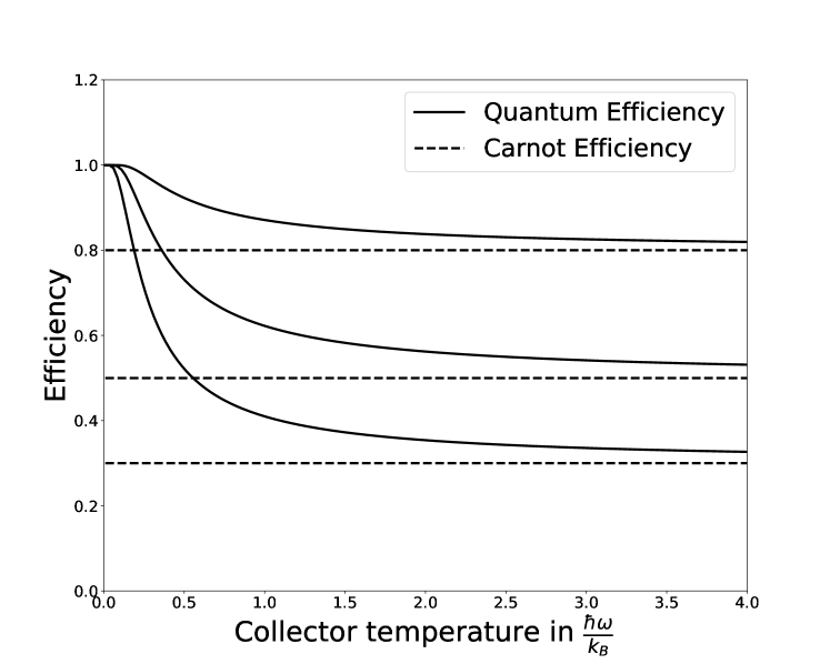
Figure 1: Steady state efficiency is plotted against collector temperature measured in $\frac{\hbar\omega_{s}}{k_{B}}$ unit at different temperatures.

The graph (Fig. 2) illustrates the relationship between the collector temperature ($T_{c}$) and the efficiency. The half efficiency is then defined as $\frac{1}{2}(1-\eta_{c})$ because the maximum value of $\eta_{s}$ is $1$. The corresponding collector temperature is then shown in Fig. 2.

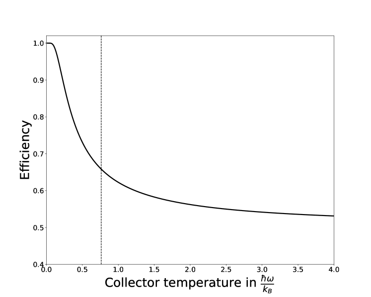
Figure 2: Half efficiency plotted for quantum efficiency vs. collector temperature as $(T_{e}=2T_{c})$.

The graph (Fig. 2) illustrates the relationship between the collector temperature ($T_{c}$) and emitter temperature ($T_{e}$) for a half-efficiency solution. As the emitter temperature (in units of $h\omega/k_{B}$) increases, the collector temperature (in units of $h\omega/k_{B}$) for which, the efficiency becomes half of its original value increases and gradually gets saturated. It is clearly shown in Fig. 3.

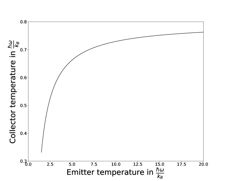
Figure 3: Solution of quantum half efficiency at different $T_{e}$ is plotted against corresponding solution of $T_{c}$.

Next we define the efficiency for thermocoherent state. Thermocoherence has been widely discussed in [19, 20, 18]. In those articles, it has been shown that the thermocoherent number density $\bar{n}_{TC}$ can be written as

$$\bar{n}^{TC} =\bar{n}^{T}+\bar{n}^{C}$$ (26)

where $\bar{n}^{T}$ is the usual thermal number density defined earlier and $\bar{n}^{C}=|\alpha|^{2}$ is the coherence number density as $\hat{a}\left|\alpha\right>=\alpha\left|\alpha\right>$ denotes the coherence state related to the system. Then the steady state efficiency for thermocoherent state can be defined as

$$\eta^{TC}_{s} =1-\frac{\bar{n}^{TC}_{c}}{\bar{n}^{TC}_{e}}~{}.$$ (27)

Using eq. (26) in the above equation, we can write

$$\eta^{TC}_{s} =1-\frac{\bar{n}_{c}^{T}+\bar{n}_{c}^{C}}{\bar{n}_{e}^{T}+\bar{n}_{e}^{C}}~{}.$$ (28)

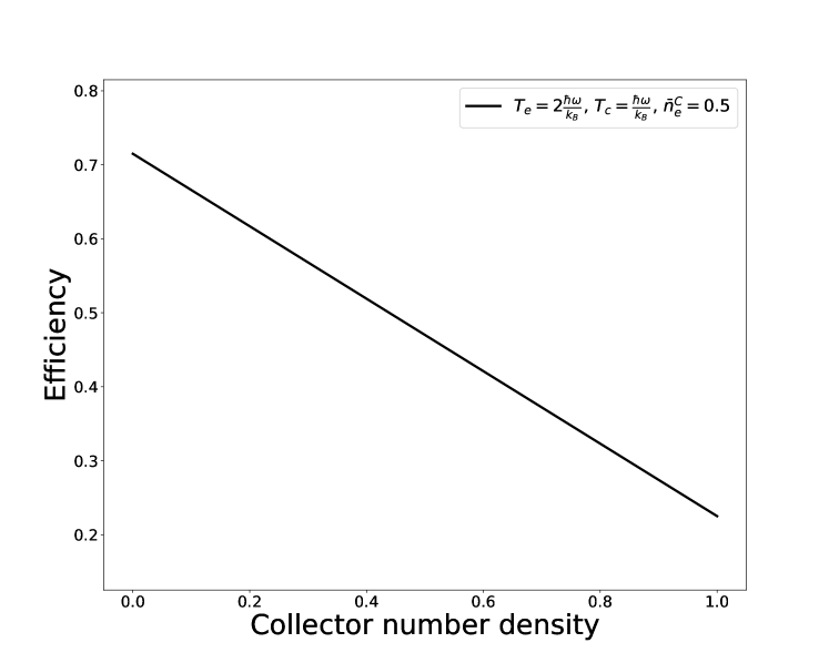
Figure 4: Steady state efficiency is plotted against collector coherence number density $\bar{n}_{c}^{C}$.

Clearly the efficiency has a negative linear relationship with collector coherence number density while other parameters are kept constant as $T_{e}=2\frac{\hbar\omega}{k_{B}T},T_{c}=\frac{\hbar\omega}{k_{B}T}$ and $\bar{n}_{e}^{C}=0.5$, indicating that as the collector number density due to coherence increases, the efficiency decreases upto a minimum value as shown in Fig. 4. The thermal densities are fixed through eq. (8).
It is clear that the efficiency can get a minimum value for certain emitter coherence number density when temperatures are kept constant. So we plot the minimum efficiency value against different value of emitter parameter in Fig. 5.

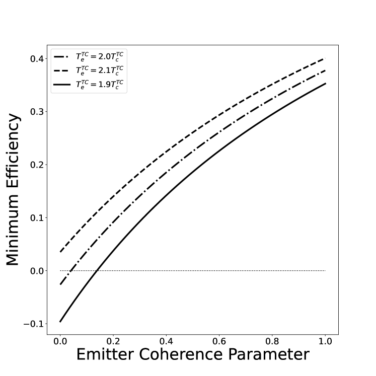
Figure 5: Minimum efficiency vs. emitter coherence number density at different emitter temperature is plotted.

Fig. 5 depicts the quantum coherence efficiency as a function of the emitter coherence number density at three different emitter temperatures for which the efficiency gets the minimum value. The graph is labeled with the condition $T^{TC}_{c}=\frac{\hbar\omega}{k_{B}}$ and $T^{TC}_{e}$ takes three different values as shown in the figure, providing additional parameters for the scenario being modeled. It is clear that the efficiency gets negative for some particular coherence number density, which is unphysical. It is shown from the graph that for $\bar{n}^{C}_{e}>0.0405$ when $T^{TC}_{e}=2\frac{\hbar\omega}{k_{B}}$ and $\bar{n}^{C}_{e}>0.138$ when $T^{TC}_{e}=1.9\frac{\hbar\omega}{k_{B}}$. Otherwise the efficiency is negative. Thus, we can conclude that the minimum value for emitter number density for the provided temperatures taken as $T^{TC}_{e}=2\frac{\hbar\omega}{k_{B}}$ and $T^{TC}_{c}=\frac{\hbar\omega}{k_{B}}$ is $0.0405$ whereas for $T^{TC}_{e}=1.9\frac{\hbar\omega}{k_{B}}$ and $T^{TC}_{c}=\frac{\hbar\omega}{k_{B}}$ is $0.138$.

IV Conclusion

The research presented here delves into the intricate dynamics governing current and efficiency within a bosonic system comprising a central unit and two reservoirs operating at distinct temperatures. Through a comprehensive formulation of the Hamiltonian for the entire system, we meticulously incorporate bosonic interactions between the central system and the reservoirs. Subsequently, by deriving a master equation, we conduct a detailed exploration of the time evolution of the density matrix of the central system, enabling a nuanced analysis of current and efficiency.
Our investigation reveals that the behavior of the current, reflecting the flow of bosons through the system, is significantly influenced by the interplay of damping coefficients and initial conditions. Within the regime of steady state, we meticulously derive an expression characterizing the efficiency of the energy transfer process. Notably, quantum effects, including the influence of temperature and the quantum correction factor, exert a pronounced impact on the overall efficiency of the system.
We make definite strides in our findings. Firstly, by utilizing the concept of flux balance, we calculate the current, which faithfully reproduces previous results. Moreover, we introduce the notion of quantum efficiency, determined through flux ratio, which remarkably gives Carnot’s efficiency as the leading term at high temperatures. Additionally, we define thermocoherence efficiency, unveiling a cut-off for certain coherence parameters. Our result also shows that the quantum efficiency can be greater than the Carnot efficiency at steady state in the high temperature limit. This result is very important for quantum technological advancement.
This research significantly contributes to our understanding of quantum thermodynamics and energy transfer processes in bosonic systems. The insights garnered hold far-reaching implications across diverse fields such as quantum computing and energy harvesting, where optimizing energy utilization is of paramount importance. Future investigations along this trajectory promise to unlock further advancements in quantum technologies, ultimately leading to systems characterized by unparalleled energy efficiency.

References

- [1] S. Çakmak, M. Çandır, and F. Altintas, “Construction of a quantum carnot heat engine cycle,” 2020.
- [2] H. T. Quan, Y.-x. Liu, C. P. Sun, and F. Nori, “Quantum thermodynamic cycles and quantum heat engines,” Phys. Rev. E, vol. 76, p. 031105, Sep 2007.
- [3] M. Y. Abd-Rabbou, A. u. Rahman, M. A. Yurischev, and S. Haddadi, “Comparative study of quantum otto and carnot engines powered by a spin,” 2023.
- [4] A. Mukherjee, S. Gangopadhyay, and A. S. Majumdar, “Unruh quantum Otto engine in the presence of a reflecting boundary,” JHEP, vol. 09, p. 105, 2022.
- [5] R. J. Glauber, “Coherent and incoherent states of the radiation field,” Physical Review, vol. 131, no. 6, p. 2766–2788, 1963.
- [6] E. Sudarshan, “Equivalence of semiclassical and quantum mechanical descriptions of statistical light beams,” Physical Review Letters, vol. 10, no. 7, p. 277, 1963.
- [7] H. J. Carmichael, Statistical Methods in Quantum Optics 1: Master Equations and Fokker-Planck Equations. Springer-Verlag Berlin Heidelberg, 2007.
- [8] W. H. Louisell, Quantum Statistical Properties of Radiation. John Wiley & Sons, Inc., 1973.
- [9] M. S. Zubairy, Quantum Optics. Cambridge University Press, 2006.
- [10] J. Weinbub and R. Kosik, “Computational perspective on recent advances in quantum electronics: From electron quantum optics to nanoelectronic devices and systems,” 2023.
- [11] D. Bhattacharyya and J. Guha, “Quantum optics and quantum computation,” 2023.
- [12] L. M. Shaker, A. Al-Amiery, W. N. R. Isahak, and W. K. Al-Azzawi, “Advancements in quantum optics: Harnessing the power of photons for next-generation technologies,” 2023.
- [13] A. Mukherjee, S. Gangopadhyay, and A. S. Majumdar, “Single and entangled atomic systems in thermal bath and the Fulling-Davies-Unruh effect,” 1 2024.
- [14] K. E. Cahill and R. J. Glauber, “Ordered expansions in boson amplitude operators,” Physical Review, vol. 177, no. 5, p. 1857–1881, 1969.
- [15] E. Verlinde, “On the origin of gravity and the laws of newton,” Journal of High Energy Physics, vol. 2011, no. 4, pp. 1–27, 2011.
- [16] N. Roos, “Entropic forces in brownian motion,” American Journal of Physics, vol. 82, no. 12, pp. 1161–1166, 2014.
- [17] J. Bhattacharya, G. Gangopadhyay, and S. Gangopadhyay, “Entropic force for quantum particles,” Physica Scripta, vol. 98, no. 8, p. 085305, 2023.
- [18] A. Karmakar and G. Gangopadhyay, “Fermionic thermocoherent state: Efficiency of electron transport,” Physical Review E, vol. 93, no. 2, p. 022141, 2016.
- [19] G. Lachs, “Theoretical aspects of mixtures of thermal and coherent radiation,” 1965.
- [20] S. Banerjee and G. Gangopadhyay, “On the quantum theory of electron transfer: Effect of potential surfaces of the reactants and products,” The Journal of chemical physics, vol. 126, no. 3, 2007.
- [21] H. B. Sun and G. J. Milburn, “Quantum open-systems approach to current noise in resonant tunneling junctions,” Physical Review B, vol. 59, no. 16, p. 10748, 1999.