Learning Macroeconomic Policies based on Microfoundations:
A Stackelberg Mean Field Game Approach

Abstract

Effective macroeconomic policies play a crucial role in promoting economic growth and social stability. This paper models the optimal macroeconomic policy problem based on the Stackelberg Mean Field Game (SMFG), where the government acts as the leader in policy-making, and large-scale households dynamically respond as followers. This modeling method captures the asymmetric dynamic game between the government and large-scale households, and interpretably evaluates the effects of macroeconomic policies based on microfoundations, which is difficult for existing methods to achieve. We also propose a solution for SMFGs, incorporating pre-training on real data and a model-free Stackelberg mean-field reinforcement learning (SMFRL) algorithm, which operates independently of prior environmental knowledge and transitions. Our experimental results showcase the superiority of the SMFG method over other economic policies in terms of performance, efficiency-equity tradeoff, and SMFG assumption analysis. This paper significantly contributes to the domain of AI for economics by providing a powerful tool for modeling and solving optimal macroeconomic policies.

1 Introduction

The formulation of macroeconomic policies is crucial for the sustained development of an economy (Schneider & Frey, 1988; Persson & Tabellini, 1999). Governments can adjust economic production, wealth distribution, social stability, and welfare through economic policies such as interest rates, taxation, and fiscal spending. Thus, how to effectively model and solve optimal macroeconomic policies, and simulate the effect of policy implementation is a very important issue. Existing research methods in economic policy primarily rely on simulations based on macroeconomic models like the Dynamic Stochastic General Equilibrium (DSGE) model (An & Schorfheide, 2007) and the Solow growth model (Brock & Taylor, 2010), or on empirical analysis (Robnik-Šikonja & Kononenko, 2003) assessing policy impacts through posterior analysis of historical data. However, these methods have limitations: (1) Difficulty in modeling dynamic interactions between the government and large-scale households, including feedback from households to policy and governmental adjustments in response to this feedback. (2) Challenge in solving the behavioral strategies of large-scale micro-agents. (3) The real economic and social world is highly complex, making it challenging for macroeconomic models to satisfy assumptions such as state transition and complete information.

Addressing these challenges, this paper employs the Stackelberg Mean Field Game (SMFG) to model optimal macroeconomic policy problems. In this framework, the government, acting as the leader, initially sets policies, while a vast number of households, as followers, respond to these policies. However, considering the large scale of the followers, it is impractical for the leader to consider each follower’s dynamic response. Consequently, followers’ action-state distribution, analogous to the overall market information in economics, is introduced as a bridge between macro-level policy and micro-level individual decisions. The optimal decisions of the leader and followers depend on the followers’ overall distribution rather than on a specific agent. This assumption is crucial for modeling optimal macroeconomic policies as SMFGs and is easily comprehensible in the real world. For example, the government lowers property taxes to stimulate a sluggish housing market. This policy alters the market’s overall state, including housing prices and market demand. Households should consider both the government’s tax policy and the overall market information when making their purchasing decisions.

Furthermore, this paper proposes a solution method for the optimal macroeconomic policy issues based on SMFG: Firstly, behavior cloning of households (followers) based on real data serves as the initialization for the policy network. This pre-training enhances the stability and performance of training and prevents ineffective solutions. Subsequently, a model-free algorithm, Stackelberg Mean-Field Reinforcement Learning (SMFRL), is introduced to solve SMFGs. This method does not rely on prior knowledge of the environment or transition information, offering advantages in solving complex economic issues. We conduct experiments on TaxAI (Mi et al., 2023), an environment for studying optimal tax policies, first to validate the performance of SMFRL against other model-free algorithms such as independent learning, MADDPG, and mean field MARL in solving SMFGs. Secondly, the paper compares the SMFG method with AI Economist, the Saez tax, the 2022 U.S. Federal tax, and free market policy, demonstrating the superiority of SMFG solutions and exploring the efficiency-equity tradeoff of these economic policies. Lastly, our tests on SMFG modeling assumptions reveal that our approach remains effective even if some households’ optimal decisions do not depend on market information. In summary, the contributions of this paper are threefold:

1. This paper is the first to model optimal macroeconomic policy problems using Stackelberg mean field games, linking macro-policies (the leader) with microfoundations (large-scale followers) through the followers’ overall distribution or average actions. It overcomes limitations such as dynamic interactions and feedback, and the dimensionality curse of large-scale households.

2. This paper employs real data for pre-training and proposes a model-free Stackelberg mean field reinforcement learning algorithm to solve SMFGs, with experimental validation of its effectiveness.

3. The paper empirically showcases the superiority of modeling and solving optimal macroeconomic policy problems by SMFGs. We also explore the efficiency-equity tradeoff in various economic policies and SMFG assumptions.

Our code is shown in an anonymous GitHub repository .

2 Related work

2.1 Economic Methods

In the field of economics, research on economic policy typically relies on theoretical model studies, empirical analysis, and econometric methods. Classic theoretical models, such as the IS-LM model (Hicks, 1980; Gali, 1992), are applicable for analyzing short-term policy effects but overlook long-term factors and price fluctuations. The aggregate demand-aggregate supply (AD-AS) model (Dutt, 2006; Lee et al., 1997) focuses on the relationship between aggregate demand and supply, integrating short-term and long-term factors, but simplifies macroeconomic dynamics. The Solow growth model (Brock & Taylor, 2010) provides a framework for economic growth but does not consider market imperfections and externalities. New Keynesian models (Blanchard & Galí, 2007; Gabaix, 2020) emphasize the stickiness of prices and wages, suitable for explaining economic fluctuations and policy interventions, but are based on strong assumptions. DSGE models (An & Schorfheide, 2007; Smets & Wouters, 2007), built on micro-foundations for macroeconomic forecasting, offer a consistent framework for policy analysis but are limited in handling nonlinearities and market imperfections. Empirical analysis (Ramesh et al., 2010; Vedung, 2017) primarily evaluates policy effects through historical data but faces limitations in data timeliness and accuracy. Econometric methods (Johnston & DiNardo, 1963; Davidson et al., 2004), such as regression and time series analysis, can quantify policy effects but are constrained by model settings and data quality.

2.2 AI for Economics

Artificial intelligence (AI), such as reinforcement learning, may offer new perspectives for solving complex economic problems (Tilbury, 2022). In terms of macroeconomics, AI Economist (Zheng et al., ) employs curriculum learning on tax policy design, Trott et al. studies the collaboration between central and local governments under COVID-19, as well as monetary policy (Hinterlang & Tänzer, ; Chen et al., 2023), international trade (Sch, 2021), market pricing (Danassis et al., 2023). However, these studies consider the government as a single agent, neglecting the dynamic response of the households to policies. Koster et al. studies democratic AI by human voting models, Yaman et al. examines the impact of social sanction rules on labor division. However, these works are based on simplified settings and remain a gap in real-world economic policy. In terms of microeconomics, Shi (2021); Rui & Shi (2022); Atashbar & Aruhan Shi (2023) study the optimal saving and consumption problems of micro-agents, and other researchers explore rational expectation equilibrium (Kuriksha, 2021; Hill et al., ), multiple equilibria under real-business-cycle (Curry et al., 2022), the emergence of barter behavior (Johanson et al., 2022), optimal asset allocation and savings strategies (Ozhamaratli & Barucca, 2022). In summary, research on macroeconomic problems still lacks a bridge framework of macro policy and microfoundations, which has drawn our attention to the Stackelberg mean field game.

2.3 Stackelberg Mean Field Game

The Stackelberg Mean Field Game models one leader and a large number of homogeneous followers, and current research can be divided into model-based methods and model-free methods. Model-based approaches typically involve complex theoretical analysis and precise mathematical modeling. For instance, Guo et al. (2022) reconceptualizes SMFGs as minimax optimization problems, while Dayanikli & Lauriere (2023); Bergault et al. (2023); Bensoussan et al. (2015); Fu & Horst (2020) initially resolve the followers’ mean field equilibrium using forward-backward stochastic functional differential equations, subsequently deriving the leader’s optimal control. Huang & Yang (2020); Bensoussan et al. (2015) explore linear-quadratic Stackelberg games. These methods provide a theoretically robust foundation but may require simplified assumptions for practical applications, particularly in complex real-world scenarios. Notably, Aurell et al. (2022) extends the mean field game model to capture epidemic dynamics, demonstrating potential applications in public health management. In contrast, model-free methods offer a way to handle complex situations that traditional numerical methods struggle with, especially in data-rich environments. Campbell et al. (2021) employs a modified deep backward stochastic differential equation (BSDE) method for solving the followers’ equilibrium, yet the leader’s choices are limited. In conclusion, we plan to use SMFGs to model macroeconomic policy issues and propose a model-free algorithm to solve this complex task.

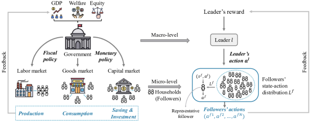
Figure 1: The mapping from optimal macroeconomic policy problems (left) to the Stackelberg Mean Field Games (right). The left represents the reality where the macro-level government implements fiscal or monetary policies to optimize GDP, welfare, or equity, and the micro-level consists of large-scale households engaging in economic activities and forming the market. In SMFGs, the government corresponds to the leader, households to the followers, and market information to the followers’ state-action distribution.

3 Macroeconomic Policy Formulation

3.1 Economic Modeling

In reality, an economy comprises at least one government and large-scale households. The diverse economic activities of households, such as production, trade, and consumption, aggregate to form the market. The government can maintain economic growth and social stability (Figure 1 left) via economic policies. The following is a mathematical model for optimizing tax policy:

Households

At timestep $t$, a household holds assets $a_{t}$. Its income $i_{t}$ consists of labor income $W_{t}e_{t}h_{t}$, and capital income $r_{t}a_{t}$. Here, $W_{t}$ and $r_{t}$ are the wage and interest rates determined by the labor and capital markets, respectively, while $e_{t}$ indicates the private education level. Households are obligated to pay taxes as per the government’s tax policy $T_{t}(i_{t},a_{t})$. Each household decides on its consumption $c_{t}\in R^{+}$, working hours $h_{t}\in R^{+}$, and next savings $a_{t+1}\in R^{+}$ to maximize long-term utility until $T_{max}$, subject to the budget constraint:

$$\max_{a_{t+1},h_{t}} \quad\mathbb{E}_{0}\sum_{t=0}^{T_{max}}u(c_{t},h_{t})$$

$$\text{s.t. }c_{t}+a_{t+1}= W_{t}e_{t}h_{t}+(1+r_{t})a_{t}-T_{t}(i_{t},a_{t}).$$

Government

The government aims to foster economic growth, maintain social equity, and enhance societal welfare through three fiscal tools: debt $B_{t}\in R^{+}$, taxation policy $T_{t}(i_{t},a_{t}):R^{+}\times R^{+}\rightarrow R^{+}$, and spending $G_{t}\in R^{+}$.

$$\max_{B_{t},T_{t},G_{t}}\quad\mathbb{E}_{0}\sum_{t=0}^{T_{max}}\left[\alpha_{1}Y_{t}+\alpha_{2}S(\mathcal{I}_{t},\mathcal{W}_{t})+\alpha_{3}\sum_{i}^{N}u_{t}^{i}\right],$$

where $\alpha_{1},\alpha_{2},\alpha_{3}$ are weight parameters reflecting the government’s preference for different objectives. Economic output (e.g., GDP) can be modeled using the Cobb–Douglas production function $Y_{t}=F(K_{t},\mathcal{L}_{t})$, with production capital $K_{t}$ and labor $\mathcal{L}_{t}$. $S(\mathcal{I}_{t},\mathcal{W}_{t})$ denotes the social equity function, where $\mathcal{I}_{t},\mathcal{W}_{t}$ are the income and wealth distributions among households. The sum of households’ utilities $\sum_{i}^{N}u_{t}^{i}$ represents the overall societal welfare.

3.2 Stackelberg Mean Field Game Modeling

In the aforementioned issue, the government (as the leader) formulates policies to guide the decisions of households (as followers), thereby collectively achieving macroeconomic objectives, such as economic growth. Households provide feedback to government policies, creating an asymmetric game with leader-follower dynamics. However, the dynamic interactions among large-scale households extend beyond the standard Stackelberg games. Therefore, this study proposes modeling the problem as a Stackelberg Mean Field Game (Figure 1), based on the following assumptions:

1. Stackelberg assumption: the government (leader) sets policies first, and households (followers) adjust their behavior based on these policies. Both the leader and followers dynamically optimize their strategies, gradually reaching equilibrium.

2. Mean field assumption: households (followers) are assumed to be homogeneous agents. The optimal policies of the leader and followers depend on the overall distribution or average behavior of the followers, rather than a specific one. For example, both governments and households should consider overall market information when making decisions in reality.

Following this, the optimal macroeconomic policy issues can be rewritten as the following game proceeding: For any given time $t\in\{0,\ldots,T_{max}\}$, the leader selects an action $a_{t}^{l}\in\mathcal{A}^{l}$ based on the leader policy $\pi_{t}^{l}(\cdot|s_{t}^{l})$, given the state $s_{t}^{l}$. Subsequently, the representative follower, located in state $s_{t}^{f}\in\mathcal{S}^{f}$, chooses an action $a_{t}^{f}\in\mathcal{A}^{f}$ according to the policy $\pi_{t}^{f}(\cdot|s_{t}^{f},a^{l}_{t})$. The sequences $\{\pi_{t}^{l}\}_{t=0}^{T-1}$ and $\{\pi_{t}^{f}\}_{t=0}^{T-1}$ are denoted as $\pi^{l}$ and $\pi^{f}$, respectively.

Followers’ Mean Field Game

Given the leader’s policy $\pi^{l}$, the SMFG is simplified into a mean field game for the followers. At time $t$, given the leader’s action $a^{l}_{t}$, the representative follower’s state $s_{t}^{f}$ and action $a_{t}^{f}$ determine the followers’ state-action distribution as $L^{f}_{t}(s_{t}^{f},a_{t}^{f})=\mathbb{P}(s_{t}^{f},a_{t}^{f})$. The representative follower then receives a reward $r^{f}(s_{t}^{f},a_{t}^{f},a_{t}^{l},L^{f}_{t})$ and transitions to the next state $s_{t+1}^{f}\sim P(\cdot|s_{t}^{f},a_{t}^{f},a_{t}^{l},L^{f}_{t})$. Each follower aims to find the optimal policy $\pi^{f}$ that maximizes his cumulative reward over the time horizon:

$$J^{f}(\pi^{l},\pi^{f},L^{f}) =\mathbb{E}^{f}\left[\sum_{t=1}^{T}r^{f}(s_{t}^{f},a_{t}^{f},a_{t}^{l},L^{f}_{t})\right]$$

$$=\mathbb{E}^{f}\left[\sum_{t=1}^{T}u(c_{t},h_{t})\right],$$

$$\text{where }c_{t} =W_{t}e_{t}h_{t}+r_{t}a_{t}-T_{t}(i_{t},a_{t})-a_{t+1},$$

where $\mathbb{E}^{f}$ denotes the expectation with respect to initial state $s_{0}^{f}\sim\mu_{0}^{f}$, $s_{t+1}^{f}\sim P(\cdot\mid s_{t}^{f},a_{t}^{f},a_{t}^{l},L^{f}_{t})$ and $a^{f}_{t}\sim\pi^{f}(\cdot\mid s_{t}^{f},a^{l}_{t})$ for each $t$. For households in economic problems, the follower’s state $s^{f}_{t}$ incorporates asset $a_{t}$ and education level $e_{t}$, and the follower’s actions $a^{f}_{t}$ include next savings $a_{t+1}$ and working hours $h_{t}$. The leader’s action $a^{l}_{t}$ denotes tax function $T_{t}(i_{t},a_{t})$, and followers’ distribution $L^{f}_{t}$ includes wage rate $W_{t}$ and interest rate $r_{t}$. Given the leader’s policy $\pi^{l}$, the best response operator of followers is defined as

$${\pi^{f}}^{*}\in\mathrm{BR}^{f}(\pi^{l},L^{f})=\arg\max_{\pi^{\prime}}J^{f}(\pi^{l},\pi^{\prime},L^{f}).$$

Stackelberg Leader’s Game

At time $t$, given the leader’s state $s^{l}_{t}$, action $a^{l}_{t}$, and the followers’ state-action distribution $L_{t}^{f}$, the leader will receive a reward $r^{l}(s_{t}^{l},a_{t}^{l},L^{f}_{t})$, and transition to a new state $s_{t+1}^{l}$ according to the transition probabilities $P(\cdot|s_{t}^{l},a_{t}^{l},L^{f}_{t})$. The leader aims to find the best policy $\pi^{l}$ to maximize the total expected rewards:

$$J^{l}(\pi^{l},\pi^{f},L^{f})=\mathbb{E}^{l}[\sum_{t=1}^{T}r^{l}(s_{t}^{l},a_{t}^{l},L^{f}_{t})],$$

$$r^{l}(s_{t}^{l},a_{t}^{l},L^{f}_{t})=\alpha_{1}Y_{t}+\alpha_{2}S(\mathcal{I}_{t},\mathcal{W}_{t})+\alpha_{3}\sum_{i}^{N}u_{t}^{i}$$

$$=\alpha_{1}F(K_{t},\mathcal{L}_{t})+\alpha_{2}S(\mathcal{I}_{t},\mathcal{W}_{t})+\alpha_{3}U(T_{t},W_{t},r_{t})$$

where $\mathbb{E}^{l}$ denotes the expectation under this probability distribution for the leader when $s_{0}^{l}\sim\mu_{0}^{l},s_{t+1}^{l}\sim P(\cdot|s_{t}^{l},a_{t}^{l},L^{f}_{t})$ and $a_{t}^{l}\sim\pi_{t}^{l}(\cdot\mid s_{t}^{l})$ for $t\in\{0,...,T-1\}$. For the government in economic problems, the leader’s state $s^{l}_{t}$ is characterized by production capital $K_{t}$, and the leader’s actions $a^{l}_{t}$ encompass government spending $G_{t}$ and a taxation policy $T_{t}(\cdot)$. The followers’ state-action distribution $L^{f}_{t}$ includes aggregate labor $\mathcal{L}_{t}$, income distribution $\mathcal{I}_{t}$, wealth distribution $\mathcal{W}_{t}$, wage rate $W_{t}$, and interest rate $r_{t}$, these all belong to market information. $U(\cdot)$ represents a measurable function for $T_{t},W_{t},r_{t}$. Therefore, we can define the leader’s best response operator given $\pi^{f},L^{f}$:

$${\pi^{l}}^{*}\in\text{BR}^{l}(\pi^{f},L^{f}):=\mathop{\arg\max}_{\pi^{l}}J^{l}(\pi^{l},\pi^{f},L^{f}).$$

We then define the transition operator $\mathcal{F}$ as $L^{f}=\mathcal{F}(\pi^{l},\pi^{f},L^{f}_{0},\mu_{0})$ if the evolution of population distribution $L$ satisfies the Mckean-Vlasov equation (1).

$$L^{f}_{t+1}(s_{t+1}^{f},a_{t+1}^{f})= \sum_{s_{t}^{l},a_{t}^{l},s_{t}^{f},a_{t}^{f}}L^{f}_{t}(s_{t}^{f},a_{t}^{f})\pi_{t}^{l}(a_{t}^{l}|s_{t}^{l})\mu_{t}^{l}(s_{t}^{l})$$ (1)

$$\quad P(s_{t+1}^{f}|s_{t}^{f},a_{t}^{f},a_{t}^{l})\pi_{t+1}^{f}(a_{t+1}^{f}|s_{t+1}^{f}).$$

$$\mu_{t+1}^{l}(s_{t+1}^{l})= \sum_{s_{t}^{l},a_{t}^{l}}\mu_{t}^{l}(s_{t}^{l})\pi_{t}^{l}(a_{t}^{l}|s_{t}^{l})P(s_{t+1}^{l}|s_{t}^{l},a_{t}^{l}).$$

Definition 3.1.

The Stackelberg mean field equilibrium is a tuple $({\pi^{l}}^{*},{\pi^{f}}^{*},{L^{f}}^{*})$, which satisfies the following conditions:

$${\pi^{l}}^{*}\in\mathrm{BR}^{l}({\pi^{f}}^{*},{L^{f}}^{*}),{\pi^{f}}^{*}\in\mathrm{BR}^{f}({\pi^{l}}^{*},{L^{f}}^{*}),$$

$${L^{f}}^{*}=\mathcal{F}({\pi^{l}}^{*},{\pi^{f}}^{*},L^{f}_{0},\mu_{0}).$$

4 Methods

Solving the optimal macroeconomic policy is very complex in the real world. Reliance solely on mathematical models for simulation and problem-solving inevitably creates a gap with actual scenarios, thus incorporating real historical data is essential. Nonetheless, a singular focus on historical data for the empirical analysis of economic policies inadequately captures the complex and asymmetric dynamics of interactions between the government and households. Therefore, our solution method is divided into two steps: firstly, we pre-train the follower’s policy based on real data using behavior cloning (BC). Secondly, this paper proposes a model-free Stackelberg Mean Field Reinforcement Learning (SMFRL) algorithm to solve the Stackelberg Mean Field Games (SMFGs) between the government and large-scale households.

4.1 Pretain by Behavior Cloning

Based on real historical data, we fetch a large number of followers’ state-action pairs $\{s^{f},a^{f}\}$ from a real-data buffer $\mathcal{D}_{real}$ for behavior cloning. For different settings of network structures, we have chosen two types of loss: when the neural network outputs a probability distribution of actions, we use the negative log-likelihood loss (NLL loss); when the neural network outputs action values, we employ the mean square error loss (MSE loss). Our goal is to find the optimal parameters $\theta$ as the follower’s policy network $\pi_{\theta}$ initialization, thereby minimizing the loss to its lowest convergence.

$$\min_{\theta}\mathcal{L}_{NLL} =-\mathbb{E}_{s^{f},a^{f}\sim\mathcal{D}}\log{\pi_{\theta}(a^{f}\mid s^{f})},$$

$$\min_{\theta}\mathcal{L}_{MSE} =\mathbb{E}_{s^{f},a^{f}\sim\mathcal{D}}\left(a^{f}-a\right)^{2}|_{a=\pi_{\theta}(s^{f})}.$$

4.2 Stackelberg Mean Field Reinforcement Learning

To solve SMFGs in sequential decision-making, we design a Stackelberg mean field reinforcement learning algorithm based on centralized training with decentralized execution. Consider a game with a leader and $N$ homogeneous follower agents. The leader makes decisions first, and all followers make simultaneous decisions after observing the leader’s actions. The leader aims to find a policy $\pi^{l}:\mathcal{S}^{l}\rightarrow\mathcal{A}^{l}$ to optimize his long-term objective, which is often challenging and requires the cooperation of all followers. Each follower agent seeks to find a policy $\pi^{f}:\mathcal{S}^{f}\times\mathcal{A}^{l}\rightarrow\mathcal{A}^{f}$ to optimize long-term utility after observing the current leader’s action $a^{l}_{t}=\pi^{l}(s^{l}_{t})$. The joint action of the leader and follower agents $\mathbf{a}_{t}=\{a^{l}_{t},a^{f1}_{t},...,a^{fN}_{t}\},a^{fi}_{t}=\pi^{f}(s^{fi}_{t})$ impacts the environment and results in a reward $\mathbf{r}_{t}=\{r^{l}_{t},r^{f1}_{t},...,r^{fN}_{t}\}$ and the next observation $\mathbf{s}_{t+1}=\{s^{l}_{t+1},s^{f1}_{t+1},...,s^{fN}_{t+1}\}$. Here the experience replay buffer $\mathcal{D}$ contains the tuples $(\mathbf{s}_{t},\mathbf{s}_{t+1},\mathbf{a}_{t},\mathbf{r}_{t},L^{f}_{t})$, recording experiences of all agents. $Q_{i}(\mathbf{s}_{t},\mathbf{a}_{t})$ is a standard centralized action-value function that takes as input the joint state $\mathbf{s}_{t}$ and joint action $\mathbf{a}_{t}$ and outputs the Q-value for agent $i$. However, due to numerous follower agents, the dimensions of both the joint state and joint action increase significantly with $N$, making the Q-function infeasible to learn. We equate the centralized action-value function $Q_{i}(\mathbf{s}_{t},\mathbf{a}_{t})$ to $\tilde{Q}_{t}(s_{t}^{l},a_{t}^{l},L_{t}^{f})$ based on mean field theory. The specific theoretical description is shown in the Appendix D.

4.3 Implementation

Furthermore, we consider deterministic policies for both a leader and its followers in a multi-agent system. Specifically, we define the leader’s policy as $\pi_{\theta^{l}}$ parameterized by $\theta^{l}$ (abbreviated as $\pi^{l}$), and a shared policy for the followers denoted as $\pi_{\theta^{f}}$ with parameters $\theta^{f}$ (abbreviated as $\pi^{f}$).

For the leader agent

The policy network $\pi_{\theta^{l}}$ of the leader agent, i.e. the actor, is trained by the sampled policy gradient (Silver et al., 2014):

$$\nabla_{\theta^{l}}J\approx\mathbb{E}_{\mathbf{s}_{t}\sim\mathcal{D}}\left[\nabla_{\theta^{l}}\pi_{\theta^{l}}(s^{l}_{t})\nabla_{a^{l}_{-}}\tilde{Q}_{\phi^{l}}(s^{l}_{t},a^{l}_{-},L^{f}_{t})|_{a^{l}_{-}=\pi_{\theta^{l}}(s^{l}_{t})}\right]$$

In the subsequent step, we employ a neural network with parameters $\phi^{l}$ to approximate the leader agent’s action-value function, denoted as $\tilde{Q}_{\phi^{l}}(s^{l}_{t},a^{l}_{t},L^{f}_{t})$ or $\tilde{Q}^{l}$ for brevity. It is updated by minimizing a loss function:

$$\mathcal{L}(\phi^{l})=\mathbb{E}_{s^{l}_{t},a^{l}_{t},L^{f}_{t},s^{l}_{t+1}\sim\mathcal{D}}\left[\left(y^{l}_{t}-\tilde{Q}_{\phi^{l}}(s^{l}_{t},a^{l}_{t},L^{f}_{t})\right)^{2}\right],$$

$$y^{l}_{t}=r_{t}^{l}+\gamma\tilde{Q}_{\phi^{l}_{-}}(s^{l}_{t+1},a^{l}_{t+1},L^{f}_{t+1})|_{a^{l}_{t+1}=\pi_{\theta^{l}_{-}}(s^{l}_{t+1})},$$ (2)

where $y^{l}_{t}$ represents the target Q value, computed using the parameters $\phi^{l}_{-}$, the next population distribution $L^{f}_{t+1}$ is based on the Mckean-Vlasov equation (1), and $\gamma$ is discount factor. Differentiating the loss function $\mathcal{L}(\phi^{l})$ yields the gradient utilized for training:

$$\nabla_{\phi^{l}}\mathcal{L}(\phi^{l})=$$

$$\mathbb{E}_{s^{l}_{t},a^{l}_{t},L^{f}_{t},s^{l}_{t+1}\sim\mathcal{D}}\left[\left(y^{l}_{t}-\tilde{Q}_{\phi^{l}}(s^{l}_{t},a^{l}_{t},L^{f}_{t})\right)\nabla_{\phi^{l}}\tilde{Q}_{\phi^{l}}(s^{l}_{t},a^{l}_{t},L^{f}_{t})\right]$$

For the representative follower agent

The policy network $\pi_{\theta^{f}}$ is trained by the policy gradient:

$$\nabla_{\theta^{f}}J\approx\mathbb{E}_{\mathbf{s}_{t},a^{l}_{t},L^{f}_{t}\sim\mathcal{D}}\Big{[}$$

$$\nabla_{\theta^{f}}\pi_{\theta^{f}}(s^{f}_{t},a^{l}_{t})\nabla_{a^{f}_{-}}\tilde{Q}_{\phi^{f}}(s^{f}_{t},a^{f}_{-},a^{l}_{t},L^{f})|_{a^{f}_{-}=\pi_{\theta^{f}}(s^{f}_{t},a^{l}_{t})}\Big{]},$$

Similar to Mean Field Approximation (Yang et al., 2018), the standard centralized action-value function $Q(\mathbf{s}_{t},\mathbf{a}_{t})$ is approximated as $\tilde{Q}_{\phi^{f}}(s^{f}_{t},a^{f}_{t},a^{l}_{t},L^{f}_{t})$ with parameters $\phi^{f}$, which is updated by minimizing the MSE loss function:

$$\mathcal{L}(\phi^{f})= \mathbb{E}_{{s}_{t}^{f},{a}_{t}^{f},a^{l}_{t},L^{f}_{t},s_{t+1}^{f}\sim\mathcal{D}}\left(y^{f}_{t}-\tilde{Q}_{\phi^{f}}(s^{f}_{t},a^{f}_{t},a^{l}_{t},L^{f}_{t})\right)^{2}$$

$$y^{f}_{t}= r^{f}_{t}+\gamma\tilde{Q}_{\phi^{f}_{-}}(s^{f}_{t+1},a^{f}_{t+1},a^{l}_{t+1},L^{f}_{t+1}),$$

where the next leader’s action $a^{l}_{t+1}=\mu_{\phi^{l}_{-}}(s^{l}_{t+1})$, the next population distribution $L^{f}_{t+1}=L(\mathbf{s}_{t+1}^{f},\mathbf{a}_{t+1}^{f})$, the next joint followers’ action $\mathbf{a}_{t+1}^{f}=\{a^{f1}_{t+1},...,a^{fN}_{t+1}\}$, $a^{fi}_{t+1}=\mu(s^{fi}_{t+1},a^{l}_{t+1})$. Differentiating the loss function $\mathcal{L}(\phi^{f})$ yields the gradient utilized for training:

$$\nabla_{\phi^{f}}\mathcal{L}(\phi^{f})=\mathbb{E}_{\mathcal{D}}\Big{[}\left(y^{f}_{t}-\tilde{Q}_{\phi^{f}}(s^{f}_{t},a^{f}_{t},a^{l}_{t},L^{f}_{t})\right)$$

$$\nabla_{\phi^{f}}\tilde{Q}_{\phi^{f}}(s^{f}_{t},a^{f}_{t},a^{l}_{t},L^{f}_{t})\Big{]}$$

The full algorithm (1) is described in the Appendix.

5 Experiment

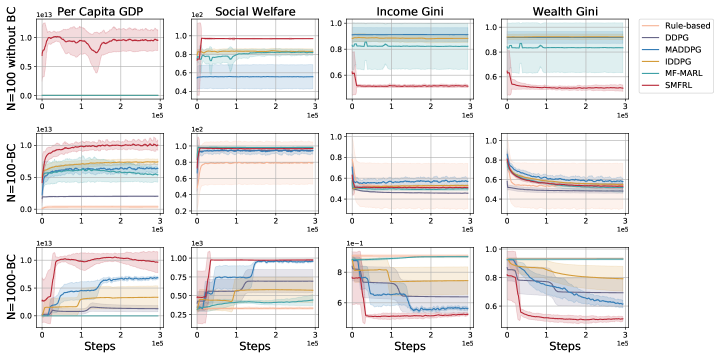
Figure 2: The training curves for 6 algorithms on 4 macroeconomic indicators, comparing settings without behavior cloning as pre-train (N=100 without BC) and with behavior cloning (N=100-BC & N=1000-BC).

Table 1: Test results for 6 algorithms on 5 indicators under 3 settings (N=100 without BC / N=100-BC / N=1000-BC).

Algorithms	Per Capita GDP	Social Welfare	Income Gini	Wealth Gini	Years
Rule-based	1.41e+05 / 3.66e+11 / 1.41e+05	69.27 / 79.23 / 334.79	0.89 / 0.52 / 0.90	0.92 / 0.53 / 0.93	1.00 / 217.45 / 1.00
DDPG	1.41e+05 / 2.03e+12 / 4.92e+11	70.91 / 94.50 / 527.09	0.88 / 0.46 / 0.75	0.92 / 0.48 / 0.79	1.00 / 299.85 / 100.68
MADDPG	4.93e+04 / 6.38e+12 / 6.82e+12	55.74 / 93.89 / 954.88	0.91 / 0.57 / 0.56	0.92 / 0.58 / 0.62	1.00 / 268.53 / 278.50
IDDPG	1.21e+05 / 7.41e+12 / 2.79e+12	83.09 / 98.16 / 512.19	0.88 / 0.53 / 0.77	0.92 / 0.55 / 0.81	1.00 / 300.00 / 100.68
MF-MARL	8.66e+07 / 5.44e+12 / 1.13e+05	82.02 / 98.21/ 440.00	0.82 / 0.50 / 0.90	0.83 / 0.52 / 0.93	75.75 / 300.00 / 1.00
SMFRL	9.59e+12 / 1.01e+13 / 9.68e+12	96.87 / 96.90 / 975.15	0.52 / 0.51 / 0.52	0.51 / 0.53 / 0.51	300.00 / 299.89 / 300.00

In this section, we conduct two important experiments in the TaxAI environment: (1) We compare the performance of the SMFRL algorithm with 5 baselines in solving SMFGs; (2) We compare the effects of the SMFG method with 5 economic policies, and discuss the efficiency-equity tradeoff and SMFG assumptions.

5.1 Environment

TaxAI (Mi et al., 2023) is a reinforcement learning simulator used for studying optimal tax policy. The environmental settings include the government promoting economic growth (i.e., GDP) through adjusting tax policy and government spending, and households optimizing labor supply and savings ratio for long-term personal utility. It is one of the few simulators for researching optimal macroeconomic policies, hence we conduct experiments on it.

5.2 Algorithmic Analysis for SMFGs

Baselines

We compare popular reinforcement learning algorithms including DDPG (Lillicrap et al., 2015) (only for leader), IDDPG (de Witt et al., 2020), MADDPG (Lowe et al., 2017), Mean Field MARL (Yang et al., 2018), and rule-based policy with our algorithm SMFRL. For more details see Appendix B.1 and Table 2.

Results

We compared SMFRL with 5 baselines in three different experimental setups: without behavior cloning as pre-training and with 100 followers (marked as N=100 without BC); with BC-based pre-training for follower agents at N=100 and N=1000 (N=100-BC; N=1000-BC). Figure 2 illustrates the training curves of 4 key macroeconomic indicators under these three settings. Each row corresponds to one setting, and each column to a macroeconomic indicator, including per capita GDP, social welfare, income Gini, and wealth Gini. A rise in per capita GDP indicates economic growth, an increase in social welfare implies happier households and a lower Gini index indicates a fairer society. Each subplot’s Y-axis represents the indicators’ values, and the X-axis represents the training steps. Table 1 displays the test results of the 6 algorithms across 5 indicators, with each column corresponding to an experimental setting.

Figure 2 and Table 1 present two experimental findings: (1) Using BC as a pre-training method for the follower’s policy enhances the algorithms’ stability and performance. Comparing settings with and without BC (the first two rows), our method, SMFRL, shows similar convergence outcomes; however, the performance of other algorithms significantly improves across all four indicators with BC-based pre-training. Furthermore, the training curves of each algorithm are more stable. (2) The SMFRL algorithm substantially outperforms other algorithms in solving SMFGs, both in large-scale followers and without pre-training scenarios. In the setting of N=100-BC, SMFRL achieved a significantly higher per capita GDP compared to other algorithms, while its social welfare and Gini index are similar to others, essentially reaching the upper limit. Besides, in N=100 without BC and N=1000-BC, SMFRL consistently obtains the most optimal solutions across all indicators.

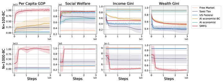
Figure 3: The training curves for 6 tax policies on 5 macroeconomic indicators (N=100 & N=1000 with BC)

5.3 Comparison of Macroeconomic Policies

Baselines

We compare free market policy, Saez tax (Saez, 2001), U.S. Federal tax , AI Economist (Zheng et al., ), and AI Economist-BC. Saez tax will provide suggestions for real-world tax reform. For more details see Appendix B.1.

Policies Results

We compare the performance of 6 policies across four economic indicators under two settings: with N=100 and N=1000 households. Figure 3 displays the training curves and Table 3 shows the test results in Appendix. Both Figure 3 and Table 3 indicate that the SMFG method significantly surpasses other policies in the task of optimizing GDP, and achieves the highest social welfare. When N=100, the Saez tax achieves the lowest income and wealth Gini coefficients, suggesting greater fairness. However, at N=1000, SMFG performs optimally across all economic indicators, while the effectiveness of other policies noticeably diminishes as the number of households increases. The Saez tax also reduces the Gini index, but not as effectively or stably as the SMFG.

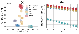
Figure 4: Comparative performance of various policies under multi-objective assessment (Efficiency-Equity).

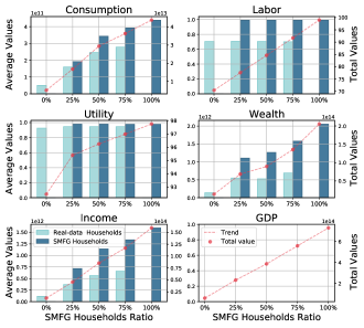
Figure 5: Comparison of micro and macroeconomic indicators at varying proportions of SMFG households, demonstrating the positive impact on the individual and overall economy of SMFG households.

Efficiency-Equity Tradeoff

In economics, the Efficiency-Equity Tradeoff is a highly debated issue. We find that our SMFG method is optimal in balancing efficiency-equity, except in cases of extreme concern for social fairness. In our study, we depict the economic efficiency (Per capita GDP) on the Y-axis and equity (wealth Gini) on the X-axis of Figure 3(a) for various policies. Different policies are represented by circles of different colors, with their sizes proportional to social welfare. Different circles of the same color correspond to different seeds. Figure 3 (a) shows that the wealth Gini indices for SMFG and AI Economist-BC are similar, but SMFG has a higher GDP, suggesting its superiority over AI Economist-BC. SMFG significantly outperforms the free market policy and AI Economist due to its higher GDPs and lower wealth Ginis. However, comparing SMFG with the Saez tax and the U.S. Federal tax policy in terms of both economic efficiency (GDP) and social equity (Gini) is challenging. Therefore, we introduce Figure 3 (b) to demonstrate the performance of different policies under various weights in a multi-objective assessment.

In Figure 3 (b), the Y-axis shows the weighted values of the multi-objective function $Y=log(\text{per capita GDP})+\alpha(\text{wealth Gini})$, and the X-axis represents the weight of the wealth Gini index. For each weight $\alpha$, we compute the multi-objective weighted values for those policies, represented as circles of different colors. Due to the logarithmic treatment of GDP in (b), when $\alpha=10$, the overall objective focuses solely on social fairness; when $\alpha=0$, the overall objective is concerned only with efficiency. Our findings in (b) reveal that only when $\alpha\geq 8$, which indicates a substantial emphasis on social equity, does the Saez tax outperform SMFG. However, SMFG consistently proves to be the most effective policy under a wide range of preference settings.

SMFG Assumption Analysis

The above experiments have already demonstrated the superiority of the SMFG method. However, the modeling and solving of SMFG rely on an important assumption: the optimal decisions of governments and households depend on the overall state information. In reality, it is natural for the government to focus on market information in decision-making, but it cannot be guaranteed that all households will consider market information in their decisions. To discuss the applicability of the SMFG method, we introduce two types of households within the same economy: those based on real data (Real-data Households) and those that focus on market information (SMFG households). We simulate the economic operations at various proportions of SMFG households: 0%, 25%, 50%, 75%, and 100%. Figure 5 displays the microeconomic indicators and macroeconomic GDP, with each subplot illustrating the average values of different economic indicators for different households (bars in left Y-axis) and their aggregate values (dots in right Y-axis). GDP, being a macroeconomic indicator, did not have corresponding values plotted for households.

The results indicate that, across all proportions, the microeconomic indicators of SMFG households, such as utility, wealth, and income, are consistently higher than Real-data households. As the proportion of SMFG households increases, there is an upward trend in economic indicators. This suggests that the presence of SMFG households positively impacts both individual and overall economic development, and our SMFG method also works when some households do not meet the assumption of focusing on market information. Therefore, governments should encourage households to pay more attention to market information in decision-making.

6 Conclusion

This paper innovatively models the optimal macroeconomic policy problem based on the Stackelberg mean field game, and proposes a solution method involving pre-training based on real data and a model-free Stackelberg mean field reinforcement learning algorithm. Our method addresses the limitations of existing approaches, including dynamic interactions and feedback between governments and households, interactions among large populations of households, and solving complex tasks without relying on environmental transitions. Experimental results have showcased the performance of the SMFG method. In conclusion, this paper contributes an effective approach to modeling and solving optimal macroeconomic policies in the field of AI for economics and AI for social good.

Impact Statements

This paper presents work whose goal is to advance the fields of AI for social good and AI for economics. Our work aims to offer suggestions and references for governments and the people, yet it must not be rashly applied to the real world. There are many potential societal consequences of our work, none of which we feel must be specifically highlighted here.

Appendix A Economic Model Details

Economic activities among households aggregate into labor markets, capital markets, goods markets, etc. In the labor market, households are the providers of labor, with the aggregate supply $S(W_{t})=\sum_{i}^{N}e_{t}^{i}h_{t}^{i}$, and firms are the demanders of labor, with the aggregate demand $D(W_{t})=\mathcal{L}_{t}$. When supply equals demand in the labor market, there exists an equilibrium price $W_{t}^{*}$ that satisfies:

$$S(W^{*}_{t})=D(W^{*}_{t}),\mathcal{L}_{t}=\sum^{N}_{i}e_{t}^{i}h_{t}^{i}.$$

In the capital market, financial intermediaries play a crucial role, lending the total deposits of households $A_{t+1}=\sum_{i}^{N}a_{t+1}$ to firms as production capital $K_{t+1}$, and purchasing government bonds $B_{t+1}$ at the interest rate $r_{t}$. The capital market clears when supply equals demand:

$$K_{t+1}+B_{t+1}-A_{t+1}=\left(r_{t}+1\right)(K_{t}+B_{t}-A_{t})$$

In the goods market, firms produce and supply goods, while all households, the government, and physical capital investments $X_{t}$ demand them. The goods market clears when:

$$Y_{t}=C_{t}+G_{t}+X_{t}$$

where $C_{t}=\sum_{i}^{N}c^{i}_{t}$ represents the total consumption of consumers, and $G_{t}$ is government spending. The supply, demand, and price represent the states of the market.

Algorithm 1 Stackelberg Mean Field Reinforcement Learning (SMFRL)

  Initialize $\tilde{Q}_{\phi^{l}},\tilde{Q}_{\phi^{l}_{-}},\tilde{Q}_{\phi^{f}},\tilde{Q}_{\phi^{f}_{-}},\pi_{\theta^{l}},\pi_{\theta^{l}_{-}},\pi_{\theta^{f}},\pi_{\theta^{f}_{-}}$.

  for epoch = 1 to M do

     Recieve initial observation $\mathbf{s}_{t}=\{s^{l}_{t},s^{f1}_{t},...,s^{fN}_{t}\}$.

     for  $t=1$ to max-epoch-length do

        For leader agent, select action $a^{l}_{t}=\pi_{\theta^{l}}(s^{l}_{t})+\mathcal{N}_{t}$; for each follower agent $i$, select action $a^{fi}=\pi_{\theta^{f}}(s^{fi}_{t},a^{l}_{t})+\mathcal{N}_{t}$ w.r.t. the current policy and exploration.

        Execute actions $\mathbf{a}_{t}=\{a^{l}_{t},a^{f1}_{t},...,a^{fN}_{t}\}$ and observe reward $\mathbf{r}_{t}=\{r_{t}^{l},r^{f1}_{t},...,r^{fN}_{t}\}$ and next observation $\mathbf{s}_{t+1}$.

        Store $(\mathbf{s}_{t},\mathbf{s}_{t+1},\mathbf{a}_{t},\mathbf{r}_{t},L^{f}_{t})$ in the replay buffer $\mathcal{D}$.

        $\mathbf{s}_{t}\leftarrow\mathbf{s}_{t+1}$.

        for j =1 to update-cycles do

           Sample a random minibatch of $N_{b}$ samples from $\mathcal{D}$.

           For the leader agent, set

$$y^{l}_{t}=r_{t}^{l}+\gamma\tilde{Q}_{\phi^{l}_{-}}(s^{l}_{t+1},a^{l}_{t+1},L^{f}_{t+1})|_{a^{l}_{t+1}=\pi_{\theta^{l}_{-}}(s^{l}_{t+1})}.$$

           Update leader’s critic net by minimizing the loss:

$$\nabla_{\phi^{l}}\mathcal{L}(\phi^{l})=\mathbb{E}_{s^{l}_{t},a^{l}_{t},L^{f}_{t},s^{l}_{t+1}\sim\mathcal{D}}\left[\left(y^{l}_{t}-\tilde{Q}_{\phi^{l}}(s^{l}_{t},a^{l}_{t},L^{f}_{t})\right)\nabla_{\phi^{l}}\tilde{Q}_{\phi^{l}}(s^{l}_{t},a^{l}_{t},L^{f}_{t})\right]$$

           Update leader’s actor by sampled policy gradient:

$$\nabla_{\theta^{l}}J\approx\mathbb{E}_{\mathbf{s}_{t}\sim\mathcal{D}}\left[\nabla_{\theta^{l}}\pi_{\theta^{l}}(s^{l}_{t})\nabla_{a^{l}_{-}}\tilde{Q}_{\phi^{l}}(s^{l}_{t},a^{l}_{-},L^{f}_{t})|_{a^{l}_{-}=\pi_{\theta^{l}}(s^{l}_{t})}\right].$$

           For the representative follower agent, set

$$y^{f}_{t}=r^{f}_{t}+\gamma\tilde{Q}_{\phi^{f}_{-}}(s^{f}_{t+1},a^{f}_{t+1},a^{l}_{t+1},L^{f}_{t+1}).$$

           Update follower’s critic by minimizing the loss:

$$\nabla_{\phi^{f}}\mathcal{L}(\phi^{f})=\mathbb{E}_{\mathcal{D}}\Big{[}\left(y^{f}_{t}-\tilde{Q}_{\phi^{f}}(s^{f}_{t},a^{f}_{t},a^{l}_{t},L^{f}_{t})\right)\nabla_{\phi^{f}}\tilde{Q}_{\phi^{f}}(s^{f}_{t},a^{f}_{t},a^{l}_{t},L^{f}_{t})\Big{]}.$$

           Update follower’s actor by policy gradient:

$$\nabla_{\theta^{f}}J\approx\mathbb{E}_{\mathbf{s}_{t},a^{l}_{t},L^{f}_{t}\sim\mathcal{D}}\Big{[}\nabla_{\theta^{f}}\pi_{\theta^{f}}(s^{f}_{t},a^{l}_{t})\nabla_{a^{f}_{-}}\tilde{Q}_{\phi^{f}}(s^{f}_{t},a^{f}_{-},a^{l}_{t},L^{f})|_{a^{f}_{-}=\pi_{\theta^{f}}(s^{f}_{t},a^{l}_{t})}\Big{]}.$$

        end for

        Update target network parameters for each agent with learning rates $\tau_{\phi}$ and $\tau_{\theta}$:

$$\begin{gathered}\phi_{-}^{l}\leftarrow\tau_{\phi}\phi^{l}+\left(1-\tau_{\phi}\right)\phi_{-}^{l}\\ \theta_{-}^{l}\leftarrow\tau_{\theta}\theta^{l}+\left(1-\tau_{\theta}\right)\theta_{-}^{l}\\ \phi_{-}^{f}\leftarrow\tau_{\phi}\phi^{f}+\left(1-\tau_{\phi}\right)\phi_{-}^{f}\\ \theta_{-}^{f}\leftarrow\tau_{\theta}\theta^{f}+\left(1-\tau_{\theta}\right)\theta_{-}^{f}\end{gathered}$$

     end for

  end for

Appendix B Additional Results

B.1 Baselines

Baselines for solving SMFGs

Current research on model-based methods for SMFG is limited by strong assumptions and simplifications, rendering them ineffective for complex problem-solving. However, there is a lack of model-free algorithms for solving SMFG in continuous decision spaces. Therefore, this study opts to compare with popular reinforcement learning algorithms, including DDPG, MADDPG, IDDPG, and mean field MARL. Table 2 provides detailed information on the algorithms used by the leader and follower agent in these baselines.

Table 2: The details of the algorithms used by the leader and follower agents in the baselines for solving SMFG.

Baselines	Follower’s Algorithm	Leader’s Algorithm
Rule-based	Random/Behavior cloning	Rule-based/Free market
DDPG	Random/Behavior cloning	DDPG
MADDPG	MADDPG	MADDPG
IDDPG	IDDPG	IDDPG
MF-MARL	Mean Field MARL	DDPG
SMFRL	SMFRL	SMFRL

Baselines for economic policies

We compare 5 economic policies with our method SMFG:

(1) Free Market: A market without policy intervention.

(2) Saez Tax (Saez, 2001): The Saex tax policy is often considered a suggestion for specific tax reforms in the real world. Details are shown in Appendix C.

(3) U.S. Federal Tax: Real data from OECD  in 2022 for this policy.

(4) AI Economist (Zheng et al., ): This is a two-level MARL method based on Proximal Policy Optimization (PPO). In the first phase, households’ policies are trained from scratch in a free-market (no-tax) environment. In the second phase, households continue to learn under an RL social planner.

(5) AI Economist-BC: For fairness in comparison, we evaluated the AI Economist method with behavior cloning as pre-training to determine its effectiveness.

B.2 Efficiency-Equity Tradeoff

In Figure 6, we also present the efficiency (per capita GDP) and equity (wealth Gini) corresponding to various algorithms for solving SMFGs. These methods result in similar Gini indices, with SMFRL achieving the highest per capita GDP. Apart from a strong emphasis on societal fairness, SMFRL emerges as the algorithm that can best strike a balance between efficiency and equity.

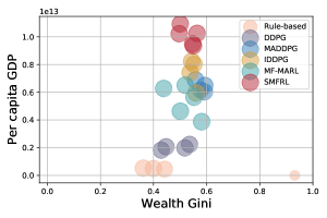
Figure 6: Comparison of macroeconomic indicators under different algorithms for solving SMFGs.

Table 3: Test results for 6 tax policies on 5 macroeconomic indicators ($N=100$ & $N=1000$).

Algorithms	$N=100$					$N=1000$
	Per Capita	Social	Income	Wealth	Years	Per Capita	Social	Income	Wealth	Years
	GDP	Welfare	Gini	Gini		GDP	Welfare	Gini	Gini
Free Market	1.37e+05	32.97	0.89	0.92	1.10	1.41e+05	334.79	0.90	0.93	1.00
Saez Tax	2.34e+12	73.82	0.21	0.38	300.00	6.35e+11	498.88	0.68	0.73	100.578
US Federal Tax	4.88e+11	94.19	0.40	0.40	289.55	1.41e+05	351.17	0.89	0.93	1.00
AI Economist-BC	4.24e+12	97.24	0.54	0.52	299.55	N/A	N/A	N/A	N/A	N/A
AI Economist	1.26e+05	72.81	0.88	0.91	1.00	N/A	N/A	N/A	N/A	N/A
SMFG	1.01e+13	96.90	0.51	0.53	299.89	9.68e+12	975.15	0.52	0.51	300.00

B.3 Behavior Cloning Experiments

This experiment conducts behavior cloning on networks for four different household policies: Multilayer Perceptron (MLP), AI economist’s network (MLP+LSTM+MLP), MF-MARL, and MADDPG network. The first two, as their network outputs are probability distributions, use negative log-likelihood loss (Figure 7 left); the latter two’s networks employ deterministic policies, hence they use mean square error loss against real data (Figure 7 right). The loss convergence curve of behavior cloning is shown in Figure 7. It can be observed that the AI economist’s network, due to its complexity, struggles to converge to near -1 like MLP. The losses corresponding to MFRL and MADDPG can converge to below 0.1.

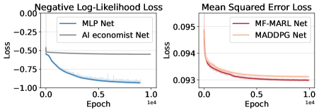
Figure 7: The behavior cloning loss for 4 networks in two loss types.

Appendix C Saez tax

The Saex tax policy is often considered a suggestion for specific tax reforms in the real world. The specific calculation method is as follows (Saez, 2001). The Saez tax utilizes income distribution $f(z)$ and cumulative distribution $F(z)$ to get the tax rates. The marginal tax rates denoted as $\tau(z)$, are expressed as a function of pretax income $z$, incorporating elements such as the income-dependent social welfare weight $G(z)$ and the local Pareto parameter $\alpha(z)$.

$$\tau(z)=\frac{1-G(z)}{1-G(z)+\alpha(z)e(z)}$$

To further elaborate, the marginal average income at a given income level $z$, normalized by the fraction of incomes above $z$, is denoted as $\alpha(z)$.

$$\alpha(z)=\frac{zf(z)}{1-F(z)}$$

The reverse cumulative Pareto weight over incomes above $z$ is represented by $G(z)$.

$$G(z)=\frac{1}{1-F(z)}\int_{z^{\prime}=z}^{\infty}p\left(z^{\prime}\right)g\left(z^{\prime}\right)\mathrm{d}z^{\prime}$$

From the above calculation formula, we can calculate $G(z)$ and $\alpha(z)$ by income distribution. We obtain the data of income and marginal tax rate through the interaction between the agent and environment and store them in the buffer. It is worth noting that the amount of buffer is fixed.

To simplify the environment, we discretize the continuous income distribution, by dividing income into several brackets and calculating a marginal tax rate $\tau(z)$ for each income range. Within each tax bracket, we determine the tax rate for that bracket by averaging the income ranges in that bracket. In other words, income levels falling within the income range are calculated as the average of that range. In particular, when calculating the top bracket rate, it is not convenient to calculate the average because its upper limit is infinite. So here $G(z)$ represents the total social welfare weight of incomes in the top bracket, when calculating $\alpha(z)$, we take the average income of the top income bracket as the average of the interval.

Elasticity $e(z)$ shows the sensitivity of the agent’s income z to changes in tax rates. Estimating elasticity is very difficult in the process of calculating tax rates, here we estimate the elasticity $e(z)$ using a regression method through income and marginal tax rates under varying fixed flat-tax systems, which produces an estimate equal to approximately 1.

$$e(z)=\frac{1-\tau(z)}{z}\frac{dz}{d(1-\tau(z))}$$

$$\log(Z)=\hat{e}\cdot\log(1-\tau)+\log\left(\widehat{Z}^{0}\right)$$

where $Z=\sum_{i}z_{i}$ when tax rates is $\tau$.

Appendix D Theoretical Proof

Proposition D.1.

The action value functions $Q_{i}$ and $\tilde{Q}_{t}$ are equivalent, i.e. $Q_{i}(\mathbf{s}_{t},\mathbf{a}_{t})=\tilde{Q}_{t}(s_{t}^{l},a_{t}^{l},L_{t}^{f})$, $\forall\mathbf{s}_{t}\in\mathcal{S}^{l}\times\{\mathcal{S}^{f}\}^{N}$, $\forall\mathbf{a}_{t}\in\mathcal{A}^{l}\times\{\mathcal{A}^{f}\}^{N}$, $\forall L_{t}^{f}\in\mathbb{P}(\mathcal{S}^{f}\times\mathcal{A}^{f})$.

Proof.

We commence by defining a partial order relation $\prec$ on $\mathcal{S}^{f}\times\mathcal{A}^{f}$. For any given vector $\mathbf{v}$, we construct a sorted counterpart $\tilde{\mathbf{v}}$, which maintains the same elements as $\mathbf{v}$ but orders them in ascending sequence based on $\prec$. For example, if $\mathbf{v}=\{(s_{1},a_{1}),(s_{2},a_{2}),(s_{3},a_{3})\}$, then $\tilde{\mathbf{v}}$ is arranged as $\{(s_{(1)},a_{(1)}),(s_{(2)},a_{(2)}),(s_{(3)},a_{(3)})\}$, where $(s_{(1)},a_{(1)})\prec(s_{(2)},a_{(2)})\prec(s_{(3)},a_{(3)})$). Exploiting the homogeneity of the follower agents, we can equate $Q(\mathbf{s}_{t},\mathbf{a}_{t})$ with $Q(s^{l}_{t},a^{l}_{t},\tilde{\mathbf{v}})$, where $\mathbf{v}$ encapsulates the joint state-action pairs of the followers, and $\tilde{\mathbf{v}}$ represents its sorted form. We further define $\mathcal{\mathbf{v}}$ as the collection of all such sorted vectors, and $\mathcal{L}$ as the ensemble of mean-field distributions. The empirical distribution of the followers’ state-action pairs, denoted as $L:\mathcal{V}\rightarrow\Delta(\mathcal{V})$, is expressed as $L^{f}_{t}(s,a)=\frac{1}{N}\sum_{i=1}^{N}\mathbb{I}_{\{(\tilde{s}_{i},\tilde{a}_{i})=(\tilde{s},\tilde{a})\}}$. The bijectiveness of the mapping $L$, ensured by the sorting process, leads to the conclusion that $Q_{t}(\mathbf{s}_{t},\mathbf{a}_{t})=Q_{t}(s^{l}_{t},a^{l}_{t},\mathbf{v})=Q_{t}(s^{l}_{t},a^{l}_{t},\tilde{\mathbf{v}})=\tilde{Q}_{t}(s^{l}_{t},a^{l}_{t},L^{f}_{t})$. ∎

References

- An & Schorfheide (2007) An, S. and Schorfheide, F. Bayesian analysis of dsge models. Econometric reviews, 26(2-4):113–172, 2007.
- Atashbar & Aruhan Shi (2023) Atashbar, T. and Aruhan Shi, R. AI and Macroeconomic Modeling: Deep Reinforcement Learning in an RBC Model, March 2023.
- Aurell et al. (2022) Aurell, A., Carmona, R., Dayanikli, G., and Lauriere, M. Optimal incentives to mitigate epidemics: a stackelberg mean field game approach. SIAM Journal on Control and Optimization, 60(2):S294–S322, 2022.
- Bensoussan et al. (2015) Bensoussan, A., Chau, M. H., and Yam, S. C. P. Mean field stackelberg games: Aggregation of delayed instructions. SIAM Journal on Control and Optimization, 53(4):2237–2266, 2015.
- Bergault et al. (2023) Bergault, P., Cardaliaguet, P., and Rainer, C. Mean field games in a stackelberg problem with an informed major player. arXiv preprint arXiv:2311.05229, 2023.
- Blanchard & Galí (2007) Blanchard, O. and Galí, J. Real wage rigidities and the new keynesian model. Journal of money, credit and banking, 39:35–65, 2007.
- Brock & Taylor (2010) Brock, W. A. and Taylor, M. S. The green solow model. Journal of Economic Growth, 15:127–153, 2010.
- Campbell et al. (2021) Campbell, S., Chen, Y., Shrivats, A., and Jaimungal, S. Deep learning for principal-agent mean field games. arXiv preprint arXiv:2110.01127, 2021.
- Chen et al. (2023) Chen, M., Joseph, A., Kumhof, M., Pan, X., and Zhou, X. Deep Reinforcement Learning in a Monetary Model, January 2023.
- Curry et al. (2022) Curry, M., Trott, A., Phade, S., Bai, Y., and Zheng, S. Analyzing Micro-Founded General Equilibrium Models with Many Agents using Deep Reinforcement Learning, February 2022.
- Danassis et al. (2023) Danassis, P., Filos-Ratsikas, A., Chen, H., Tambe, M., and Faltings, B. AI-driven Prices for Externalities and Sustainability in Production Markets, January 2023.
- Davidson et al. (2004) Davidson, R., MacKinnon, J. G., et al. Econometric theory and methods, volume 5. Oxford University Press New York, 2004.
- Dayanikli & Lauriere (2023) Dayanikli, G. and Lauriere, M. A machine learning method for stackelberg mean field games. arXiv preprint arXiv:2302.10440, 2023.
- de Witt et al. (2020) de Witt, C. S., Gupta, T., Makoviichuk, D., Makoviychuk, V., Torr, P. H., Sun, M., and Whiteson, S. Is independent learning all you need in the starcraft multi-agent challenge? arXiv preprint arXiv:2011.09533, 2020.
- Dutt (2006) Dutt, A. K. Aggregate demand, aggregate supply and economic growth. International review of applied economics, 20(3):319–336, 2006.
- Fu & Horst (2020) Fu, G. and Horst, U. Mean-field leader-follower games with terminal state constraint. SIAM Journal on Control and Optimization, 58(4):2078–2113, 2020.
- Gabaix (2020) Gabaix, X. A behavioral new keynesian model. American Economic Review, 110(8):2271–2327, 2020.
- Gali (1992) Gali, J. How well does the is-lm model fit postwar us data? The Quarterly Journal of Economics, 107(2):709–738, 1992.
- Guo et al. (2022) Guo, X., Hu, A., and Zhang, J. Optimization frameworks and sensitivity analysis of stackelberg mean-field games. arXiv preprint arXiv:2210.04110, 2022.
- Hicks (1980) Hicks, J. Is-lm: an explanation. Journal of post Keynesian economics, 3(2):139–154, 1980.
- (21) Hill, E., Bardoscia, M., and Turrell, A. Solving Heterogeneous General Equilibrium Economic Models with Deep Reinforcement Learning. URL http://arxiv.org/abs/2103.16977.
- (22) Hinterlang, N. and Tänzer, A. Optimal Monetary Policy Using Reinforcement Learning. URL https://papers.ssrn.com/abstract=4025682.
- Huang & Yang (2020) Huang, M. and Yang, X. Mean field stackelberg games: State feedback equilibrium. IFAC-PapersOnLine, 53(2):2237–2242, 2020.
- Johanson et al. (2022) Johanson, M. B., Hughes, E., Timbers, F., and Leibo, J. Z. Emergent Bartering Behaviour in Multi-Agent Reinforcement Learning, May 2022.
- Johnston & DiNardo (1963) Johnston, J. and DiNardo, J. Econometric methods. 1963.
- (26) Koster, R., Balaguer, J., Tacchetti, A., Weinstein, A., Zhu, T., Hauser, O., Williams, D., Campbell-Gillingham, L., Thacker, P., Botvinick, M., and Summerfield, C. Human-centred mechanism design with Democratic AI. 6(10):1398–1407. ISSN 2397-3374. doi: 10.1038/s41562-022-01383-x. URL https://www.nature.com/articles/s41562-022-01383-x.
- Kuriksha (2021) Kuriksha, A. An Economy of Neural Networks: Learning from Heterogeneous Experiences, October 2021.
- Lee et al. (1997) Lee, K., Pesaran, M. H., and Smith, R. Growth and convergence in a multi-country empirical stochastic solow model. Journal of applied Econometrics, 12(4):357–392, 1997.
- Lillicrap et al. (2015) Lillicrap, T. P., Hunt, J. J., Pritzel, A., Heess, N., Erez, T., Tassa, Y., Silver, D., and Wierstra, D. Continuous control with deep reinforcement learning. arXiv preprint arXiv:1509.02971, 2015.
- Lowe et al. (2017) Lowe, R., Wu, Y. I., Tamar, A., Harb, J., Pieter Abbeel, O., and Mordatch, I. Multi-agent actor-critic for mixed cooperative-competitive environments. Advances in neural information processing systems, 30, 2017.
- Mi et al. (2023) Mi, Q., Xia, S., Song, Y., Zhang, H., Zhu, S., and Wang, J. Taxai: A dynamic economic simulator and benchmark for multi-agent reinforcement learning. arXiv preprint arXiv:2309.16307, 2023.
- Ozhamaratli & Barucca (2022) Ozhamaratli, F. and Barucca, P. Deep Reinforcement Learning for Optimal Investment and Saving Strategy Selection in Heterogeneous Profiles: Intelligent Agents working towards retirement, June 2022.
- Persson & Tabellini (1999) Persson, T. and Tabellini, G. Political economics and macroeconomic policy. Handbook of macroeconomics, 1:1397–1482, 1999.
- Ramesh et al. (2010) Ramesh, M., Wu, X., Howlett, M., and Fritzen, S. The public policy primer: Managing the policy process. 2010.
- Robnik-Šikonja & Kononenko (2003) Robnik-Šikonja, M. and Kononenko, I. Theoretical and empirical analysis of relieff and rrelieff. Machine learning, 53:23–69, 2003.
- Rui & Shi (2022) Rui and Shi. Learning from zero: How to make consumption-saving decisions in a stochastic environment with an AI algorithm, February 2022.
- Saez (2001) Saez, E. Using elasticities to derive optimal income tax rates. The review of economic studies, 68(1):205–229, 2001.
- Sch (2021) Sch, A. A. O. Intelligence in the economy: Emergent behaviour in international trade modelling with reinforcement learning. 2021.
- Schneider & Frey (1988) Schneider, F. and Frey, B. S. Politico-economic models of macroeconomic policy: A review of the empirical evidence. Political business cycles, pp. 239–275, 1988.
- Shi (2021) Shi, R. A. Can an AI agent hit a moving target. arXiv preprint arXiv, 2110, 2021.
- Silver et al. (2014) Silver, D., Lever, G., Heess, N., Degris, T., Wierstra, D., and Riedmiller, M. Deterministic policy gradient algorithms. In International conference on machine learning, pp. 387–395. Pmlr, 2014.
- Smets & Wouters (2007) Smets, F. and Wouters, R. Shocks and frictions in us business cycles: A bayesian dsge approach. American economic review, 97(3):586–606, 2007.
- Tilbury (2022) Tilbury, C. Reinforcement learning in macroeconomic policy design: A new frontier? arXiv preprint arXiv:2206.08781, 2022.
- (44) Trott, A., Srinivasa, S., Haneuse, S., and Zheng, S. Building a Foundation for Data-Driven, Interpretable, and Robust Policy Design using the AI Economist. URL http://arxiv.org/abs/2108.02904.
- Vedung (2017) Vedung, E. Public policy and program evaluation. Routledge, 2017.
- (46) Yaman, A., Leibo, J. Z., Iacca, G., and Lee, S. W. The emergence of division of labor through decentralized social sanctioning. URL http://arxiv.org/abs/2208.05568.
- Yang et al. (2018) Yang, Y., Luo, R., Li, M., Zhou, M., Zhang, W., and Wang, J. Mean field multi-agent reinforcement learning. In International conference on machine learning, pp. 5571–5580. PMLR, 2018.
- (48) Zheng, S., Trott, A., Srinivasa, S., Parkes, D. C., and Socher, R. The AI Economist: Taxation policy design via two-level deep multiagent reinforcement learning. 8(18):eabk2607. doi: 10.1126/sciadv.abk2607. URL https://www.science.org/doi/10.1126/sciadv.abk2607.