Align and Distill: Unifying and Improving Domain Adaptive Object Detection

Abstract

Object detectors often perform poorly on data that differs from their training set. Domain adaptive object detection (DAOD) methods have recently demonstrated strong results on addressing this challenge. Unfortunately, we identify systemic benchmarking pitfalls that call past results into question and hamper further progress: (a) Overestimation of performance due to underpowered baselines, (b) Inconsistent implementation practices preventing transparent comparisons of methods, and (c) Lack of generality due to outdated backbones and lack of diversity in benchmarks. We address these problems by introducing: (1) A unified benchmarking and implementation framework, Align and Distill (ALDI), enabling comparison of DAOD methods and supporting future development, (2) A fair and modern training and evaluation protocol for DAOD that addresses benchmarking pitfalls, (3) A new DAOD benchmark dataset, CFC-DAOD, enabling evaluation on diverse real-world data, and (4) A new method, ALDI++, that achieves state-of-the-art results by a large margin. ALDI++ outperforms the previous state-of-the-art by +3.5 AP50 on Cityscapes $\rightarrow$ Foggy Cityscapes, +5.7 AP50 on Sim10k $\rightarrow$ Cityscapes (where ours is the only method to outperform a fair baseline), and +2.0 AP50 on CFC Kenai $\rightarrow$ Channel. Our framework, dataset, and state-of-the-art method offer a critical reset for DAOD and provide a strong foundation for future research.

1 Introduction

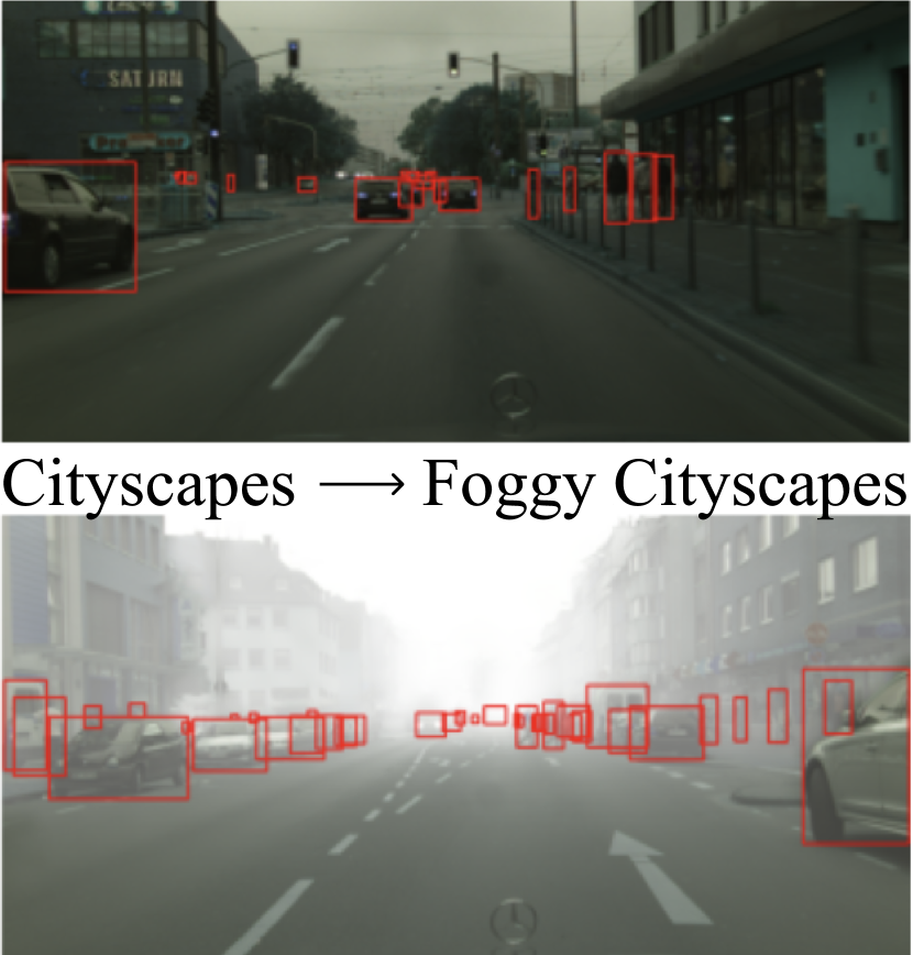
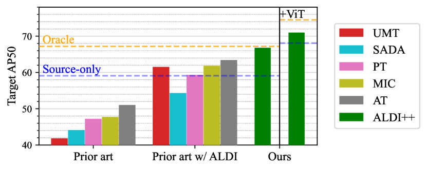
Figure 1: ALDI achieves state-of-the-art performance in domain adaptive object detection (DAOD) and provides a unified framework for fair comparison. We show: (1) Inconsistent implementation practices give the appearance of steady progress in DAOD (left bars [12, 10, 8, 26, 34]); reimplementation and fair comparison with ALDI shows less difference between methods than previously reported (middle bars); (2) A fairly constructed source-only model (blue line) outperforms many existing DAOD methods, indicating less progress has been made than previously reported; and a proper oracle (orange line) outperforms all existing methods, in contrast to previously-published results; and (3) Our proposed method ALDI++ (green bars) achieves state-of-the-art performance on DAOD benchmarks such as Cityscapes $\rightarrow$ Foggy Cityscapes and is complementary to ongoing advances in object detection like VitDet [33].

The challenge of DAOD. Modern object detector performance, though excellent across many benchmarks [36, 53, 52, 3, 49, 46], often severely degrades when test data exhibits a distribution shift with respect to training data [41]. For instance, detectors do not generalize well when deployed in new environments in environmental monitoring applications [30, 53]. Similarly, models in medical applications perform poorly when deployed in different hospitals or on different hardware than they were trained [55, 19]. Unfortunately, in real-world applications it is often difficult, expensive, or time-consuming to collect the additional annotations needed to address such distribution shifts in a supervised manner. An appealing option in these scenarios is unsupervised domain adaptive object detection (DAOD), which attempts to improve detection performance when moving from a “source” domain (used for training) to a “target” domain (used for testing) [32, 29] without the use of target-domain supervision.

The current paradigm. The research community has established a set of standard benchmark datasets and methodologies that capture the deployment challenges motivating DAOD. Benchmarks consist of labeled data that is divided into two sets: a source and a target, each originating from different domains. DAOD methods are trained with source-domain images and labels, as in traditional supervised learning, and have access to unlabeled target domain images. The target-domain labels are not available for training.

To measure DAOD methods’ performance, researchers use source-only models and oracle models as points of reference. Source-only models—sometimes also referred to as baselines—are trained with source-domain data only, representing a lower bound for performance without domain adaptation. Oracle models are trained with supervised target-domain data, representing a fully-supervised upper bound. The goal in DAOD is to close the gap between source-only and oracle performance without target-domain supervision.

Impediments to progress. Recently-published results indicate DAOD is exceptionally effective, doubling the performance of source-only models and even outperforming fully-supervised oracles [34, 8, 5]. However, upon close examination we discover problems with current benchmarking practices that call these results into question:

P1: Improperly constructed source-only and oracle models, leading to overestimation of performance gains. We find that source-only and oracle models are consistently constructed in a way that does not properly isolate domain-adaptation-specific components, leading to misattribution of performance improvements. We show that when source-only and oracle models are fairly constructed—i.e. use the same architecture and training settings as DAOD methods—no existing methods outperform oracles and many methods do not even outperform source-only models (Fig. 1), in stark contrast to claims made by recent work. These results mean we do not have an accurate measure of the efficacy of DAOD.

P2: Inconsistent implementation practices preventing transparent comparisons of methods. We find existing DAOD methods are built using a variety of different object detection libraries with inconsistent training settings, making it difficult to determine whether performance improvements come from new DAOD methods or simply improved hyperparameters. We find that tweaking these hyperparameters—whose values often differ between methods yet are not reported in papers—can lead to a larger change in performance than the proposed methods themselves (see Sec. 6.3), thus we cannot take reported advancements at face value. Without the ability to make fair comparisons we cannot transparently evaluate contributions nor make principled methodological progress.

P3: (a) Lack of diverse benchmarks and (b) outdated model architectures, leading to overestimation of methods’ generality. DAOD benchmarks have focused largely on urban driving scenarios with synthetic distribution shifts [48, 28], and methods continue to use outdated detector architectures for comparison with prior work [9]. The underlying assumption is that methods will perform equivalently across application domains and backbone architectures. We show that in fact the ranking of methods changes across benchmarks and architectures, revealing that published results may be uninformative for practitioners using modern architectures and real-world data.

A critical reset for DAOD research. DAOD has the potential for impact in a range of real-world applications, but these systemic benchmarking pitfalls impede progress. We aim to address these problems and lay a solid foundation for future progress in DAOD with the following contributions:

1. Align and Distill (ALDI), a unified benchmarking and implementation framework for DAOD. In order to enable fair comparisons, we first identify key themes in prior work (Sec. 2) and unify common components into a single state-of-the-art framework, ALDI (Sec. 3). ALDI facilitates detailed study of prior art and streamlined implementation of new methods, supporting future research.

2. A fair and modern training protocol for DAOD methods, enabled by ALDI. We provide quantitative evidence of the benchmarking pitfalls we identify and propose an updated training and evaluation protocol to address them (Sec. 6.1). This enables us to set more realistic and challenging targets for the DAOD community and perform the first fair comparison of prior work in DAOD (Sec. 6.2).

3. A new benchmark dataset, CFC-DAOD, sourced from a real-world adaptation challenge in environmental monitoring (Sec. 5). CFC-DAOD increases the diversity of DAOD benchmarks and is notably larger than existing options. We show that the ranking of methods changes across different benchmarks (Sec. 6.2), thus the community will benefit from an additional point of comparison.

4. A new method, ALDI++, that achieves state-of-the-art results by a large margin. Using the same model settings across all benchmarks, ALDI++ outperforms the previous state-of-the-art by +3.5 AP50 on Cityscapes $\rightarrow$ Foggy Cityscapes, +5.7 AP50 on Sim10k $\rightarrow$ Cityscapes (where ours is the only method to outperform a fair source-only model), and +2.0 AP50 on CFC Kenai $\rightarrow$ Channel.

2 Related Work

Two methodological themes have dominated recent DAOD research: feature alignment and self-training/self-distillation. We first give an overview of these themes and previous efforts to combine them, and then use commonalities to motivate our unified framework, Align and Distill, in Sec. 3.

Feature alignment in DAOD. Feature alignment methods aim to make target-domain data “look like” source-domain data, reducing the magnitude of the distribution shift. The most common approach utilizes an adversarial learning objective to align the feature spaces of source and target data [16, 10, 9, 57]. Faster R-CNN in the Wild [9] utilizes adversarial networks at the image and instance level. SADA [10] extends this to multiple adversarial networks at different feature levels. Other approaches propose mining for discriminative regions [57], weighting local and global features differently [47], incorporating uncertainty [40], and using attention networks [51]. Alignment at the pixel level has also been proposed using image-to-image translation techniques to modify input images directly [12].

Self-training/self-distillation in DAOD. Self-training methods use a “teacher” model to predict pseudo-labels on target-domain data that are then used as training targets for a “student” model. Self-training can be seen as a type of self-distillation [43, 6], which is a special case of knowledge distillation [25, 7] where the teacher and student models share the same architecture. Most recent self-training approaches in DAOD are based on the Mean Teacher [50] framework, in which the teacher model is updated as an exponential moving average (EMA) of the student model’s parameters. Extensions to Mean Teacher for DAOD include: MTOR, which utilizes graph structure to enforce student-teacher feature consistency [4], Probabilistic Teacher (PT), which uses probabilistic localization prediction and soft distillation losses [8], and Contrastive Mean Teacher (CMT), which uses MoCo [21] to enforce student-teacher feature consistency [5].

Combining feature alignment and self-training. Several approaches utilize both feature alignment and self-training/self-distillation, motivating our unified framework. Unbiased Mean Teacher (UMT) [12] uses mean teacher in combination with image-to-image translation to align source and target data at the pixel level. Adaptive Teacher (AT) [55] uses mean teacher with an image-level discriminator network. Masked Image Consistency (MIC) [26] uses mean teacher, SADA, and a masking augmentation to enforce teacher-student consistency. Because these methods were implemented in different codebases using different training recipes and hyparameter settings, it is unclear which contributions are most effective and to what extent feature alignment and self-training are complementary. We address these issues by reimplementing these approaches in the ALDI framework and perform fair comparisons and ablation studies in Sec. 6.

DAOD datasets. Cityscapes (CS) $\rightarrow$ Foggy Cityscapes (FCS) [11, 48] is a popular DAOD benchmark that emulates domain shift caused by changes in weather in urban driving scenarios. The dataset contains eight vehicle and person classes. Sim10k $\rightarrow$ CS [28] poses a Sim2Real challenge, adapting from video game imagery to real-world imagery. The benchmark focuses on a single class, “car”. Other common tasks include adapting from real imagery in PascalVOC [15] to clip art and watercolor imagery [27]. We report results on CS $\rightarrow$ FCS and Sim10k $\rightarrow$ CS due to their widespread popularity in the DAOD literature and focus on real applications. We note that existing benchmarks reflect a relatively narrow set of potential DAOD applications. To study whether methods generalize outside of urban driving scenarios, in Sec. 5 we introduce a novel dataset sourced from a real-world adaptation challenge in environmental monitoring, where imagery is much different from existing benchmarks.

3 Align and Distill (ALDI): Unifying DAOD

We first introduce Align and Distill (ALDI), a new benchmarking and implementation framework for DAOD. ALDI unifies existing approaches in a common framework, enabling fair comparisons and addressing P2. Inconsistent implementation practices, while also providing the foundation for development of a new method ALDI++ that achieves state-the-art performance (Sec. 4, Sec. 6.2). The framework is visualized in Fig. 2. All components are ablated in Sec. 6.3.

Data. DAOD involves two datasets: a labeled source dataset $X_{src}$ and an unlabeled target dataset $X_{tgt}$. Each training step, a minibatch of size $B$ is constructed containing both $B_{src}$ source images and $B_{tgt}$ target images.

Models. A student model $\theta_{stu}$ and a teacher model $\theta_{tch}$ are initialized with the same weights, typically obtained through supervised pretraining on ImageNet, COCO, or $X_{src}$. Pretraining on $X_{src}$ is often referred to as “burn-in.” The student is trained through backpropagation. The teacher’s weights are not updated by backpropagation, rather they are updated to be the EMA of student weights [50].

Training involves three objectives:

1. Supervised training with source data. Each labeled source sample $x_{src,i}$ is transformed by some $t\sim T_{src}$, the set of possible source-domain transformations, then passed through the student model to obtain a supervised loss $L_{sup}$ given ground truth targets $y_{src,i}$. In our case $L_{sup}$ are Faster R-CNN losses [44].

2. Self-distillation with target data. Each unlabeled target sample $x_{tgt,i}$ passes through both the teacher and student models. The teacher’s predictions $\hat{p}_{tgt,i}$ act as distillation targets for the student’s predictions $p_{tgt,i}$, resulting in distillation losses $L_{distill}$ that are backpropagated through the student. Before computing $L_{distill}$ the teacher’s outputs are postprocessed to be either soft (e.g. logits or softmax outputs) or hard (e.g. thresholded pseudo-label) targets.

Before passing through the teacher, $x_{tgt,i}$ is transformed by some $\hat{t}\sim\hat{T}_{weak}$, a set of “weak” transformations—e.g. random horizontal flipping—that allow the teacher to provide high quality predictions $\hat{p}_{tgt}$. The same image is also passed to the student, this time transformed by $t\sim T_{tgt}$ which typically contains “stronger” augmentations such as color jitter or random erasing.

Table 1: ALDI unifies and extends existing work. We show settings to reproduce five prior works and our method ALDI++. See Fig. 2 and Sec. 3 for more details. Burn-in: fixed duration (Fixed), our approach (Ours, Sec. 4). Augs. $T_{src},T_{tgt}$: Random flip (F), multi-scale (M), crop & pad (CP), color jitter (J), cutout [13] (C), MIC [26]. ${\frac{1}{2}}$: augs used on half the images in the batch. $\frac{B_{tgt}}{B}$: Target-domain portion of minibatch of size $B$. Postprocess: Processing of teacher preds before distillation: sigmoid/softmax (Sharpen), sum class preds for pseudo-objectness (Sum), conf. thresholding (Thresh), NMS. $L_{distill}$: Distillation losses: hard pseudo-labels (Hard), continuous targets (Soft). $L_{align}$: Feature alignment losses: image-level adversarial (Img), instance-level adversarial (Inst), image-to-image translation (Img2Img). ^†: settings used in ALDI implementation (last column) but not in the original implementation (second-to-last column). ^at: source-only and oracle results sourced from [34].

Method	$\theta_{stu},\theta_{tch}$				Post-			AP50FCS	AP50FCS
	Burn-in	$T_{src}$	$T_{tgt}$	$\frac{B_{tgt}}{B}$	process	$L_{distill}$	$L_{align}$	(Reported)	(w/ ALDI)
Source-only	–	F, M†, C†, E†	–	0.0	–	–	–	at23.5	59.1
SADA [10]	–	F	F	0.5	–	–	Img, Inst	44.0	54.2
PT [8]	Fixed	F	F, J, C	0.3	Sharpen, Sum	Soft	–	47.1	59.2
UMT [12]	–	–	CP, J	0.5	Thresh, NMS	Hard	Img2Img	41.7	61.4
MIC [26]	–	F	F, J, MIC	0.5	Thresh, NMS	Hard	Img, Inst	47.6	61.7
AT [34]	Fixed	F, J${}^{\frac{1}{2}}$, C${}^{\frac{1}{2}}$	F, J, C	0.3	Thresh, NMS	Hard	Img	50.9	63.3
ALDI++	Ours	F, M, J, C	F, M, J, MIC	0.5	Sharpen	Soft	–	–	66.8
Oracle	–	–	F, M†, J†, C†	1.0	–	–	–	at42.7	67.2

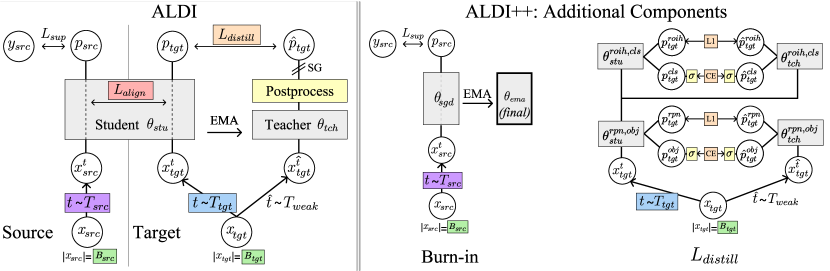
Figure 2: (Left) The ALDI student-teacher framework for DAOD. Each training step (moving left to right and bottom to top): (1) Sample $B_{src}$ labeled source images $x_{src}$; transform by $t\sim T_{src}$; pass to student; compute supervised loss $L_{sup}$ using ground-truth labels $y_{src}$. (2) Sample $B_{tgt}$ unlabeled target images $x_{tgt}$; transform by $t\sim T_{tgt}$; pass to student to get preds $p_{tgt}$. Compute alignment objectives $L_{align}$ using $x_{src}$ and $x_{tgt}$. (3) Pass same unlabeled target data $x_{tgt}$, weakly transformed, to teacher; postprocess to obtain teacher preds $\hat{p}_{tgt}$. Compute distillation loss $L_{distill}$ between teacher and student preds. Use stop gradient (SG) on teacher model; update teacher to the EMA of student’s weights. (Middle, Right) ALDI++ (Sec. 4) introduces two new methods to achieve state-of-the-art performance: (Middle) A robust burn-in strategy utilizing strong augmentations and EMA, and (Right) Multi-task soft distillation losses to train the student using teacher outputs at all detector stages. $\sigma$: sigmoid or softmax for binary cross-entropy and cross entropy losses, respectively.

3. Feature alignment. $x_{src,:}$ and $x_{tgt,:}$ are “aligned” via an alignment objective $L_{align}$ that enforces invariance across domains either at the image or feature level.

Unification of prior work. We demonstrate the generality of our framework by reimplementing five recently-proposed methods on top of ALDI for fair comparison: UMT [12], SADA [10], PT [8], MIC [26], and AT [34]. In Tab. 1 we enumerate the settings required to reproduce each method.

4 ALDI++: Improving DAOD

We next propose two novel enhancements to the Align and Distill approach, resulting in a new method ALDI++. We show in Sec. 6.2 that these enhancements lead to state-of-the-art results, and ablate each component in Sec. 6.3.

1. Robust burn-in. First we propose a new “burn-in” strategy for pretraining a teacher model $\theta_{tch}$ on source-only data $X_{src}$. A key challenge in student-teacher methods is improving target-domain pseudo-label quality. We point out that psuedo-label quality in the early stages of self-training is largely determined by the out-of-distribution (OOD) generalization capabilities of the initial teacher model $\theta^{init}_{tch}$, and thus propose a training strategy aimed at improving OOD generalization during burn-in. We add strong data augmentations including random resizing, color jitter, and random erasing, and keep an EMA copy of the model during burn-in, two strategies that have previously been shown to improve OOD generalization and robustness [1, 2, 18]. We are the first to utilize these strategies for DAOD burn-in.

2. Multi-task soft distillation. Most prior work utilizes confidence thresholding and non-maximum suppression to generate “hard” pseudo-labels from teacher predictions $\hat{p}_{tgt}$ (see Tab. 1). However in object detection this strategy is sensitive to the confidence threshold chosen, leading to both false positive and false negative errors that harm self-training [31]. We take inspiration from the knowledge distillation literature and propose instead using “soft” distillation losses—i.e. using teacher prediction scores as targets without thresholding—allowing us to eliminate the confidence threshold hyperparameter.

We distill each task of Faster R-CNN—Region Proposal Network localization ($rpn$) and objectness ($obj$), and Region-of-Interest Heads localization ($roih$) and classification ($cls$)—independently. At each stage, the teacher provides distillation targets for the same set of input proposals used by the student—i.e. anchors $A$ in the first stage, and student region proposals $p^{rpn}_{tgt}$ in the second stage: $$p^{rpn,obj}_{tgt}=\theta^{rpn,obj}_{stu}(A,x^{t}_{tgt})$$ (1) $$\hat{p}^{rpn,obj}_{tgt}=\theta^{rpn,obj}_{tch}(A,x^{\hat{t}}_{tgt})$$ (2) $$p^{roih,cls}_{tgt}=\theta^{roih,cls}_{stu}(p^{rpn}_{tgt},x^{t}_{tgt})$$ (3) $$\hat{p}^{roih,cls}_{tgt}=\theta^{roih,cls}_{tch}(p^{rpn}_{tgt},x^{\hat{t}}_{tgt})$$ (4)

At each iteration, student distillation losses $L_{distill}$ are computed as:

$$L^{rpn}_{distill}=\lambda_{0}L_{rpn}(p^{rpn}_{tgt},\hat{p}^{rpn}_{tgt})+\lambda_{1}L_{obj}(p^{obj}_{tgt},\hat{p}^{obj}_{tgt})$$ (5)

$$L^{roih}_{distill}=\lambda_{2}L_{roih}(p^{roih}_{tgt},\hat{p}^{roih}_{tgt})+\lambda_{3}L_{cls}(p^{cls}_{tgt},\hat{p}^{cls}_{tgt})$$ (6)

$$L_{distill}=L^{rpn}_{distill}+L^{roih}_{distill}$$ (7)

Where $L_{rpn}$ and $L_{roih}$ are the smooth L1 loss and $L_{obj}$ and $L_{cls}$ are the cross-entropy loss, and $\lambda_{0\dots 3}=1$ by default. See Fig. 2 for a visual depiction. We include more implementation details in the supplemental material.

One prior DAOD work, PT [8], has also used soft distillation losses, however we note two shortcomings our method addresses: (1) PT requires a custom “Probabilistic R-CNN” architecture for distillation, while our approach is general and can work with any two-stage detector, and (2) PT uses $\hat{p}^{cls}$ as an indirect proxy for distilling $p^{obj}$, while our approach is able to distill each task directly.

5 The CFC-DAOD Dataset

Next we introduce our dataset contribution, CFC-DAOD, addressing P3: (a) Lack of diverse benchmarks leading to overestimation of methods’ generality.

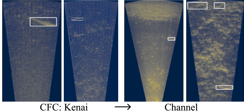
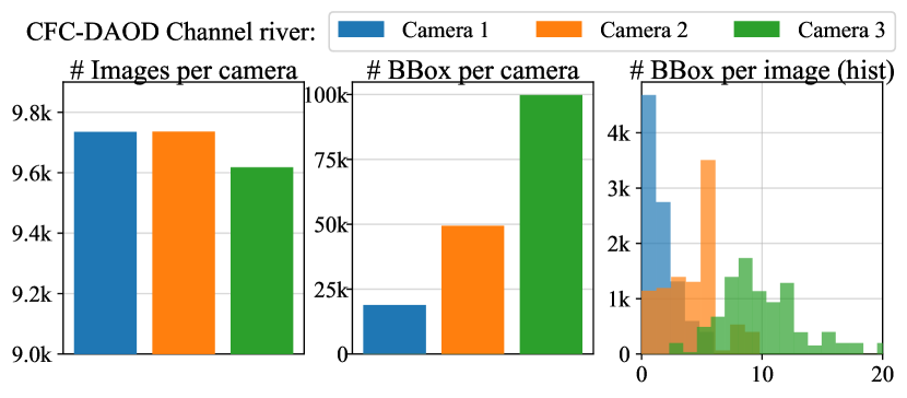
Figure 3: The CFC-DAOD benchmark focuses on detecting fish (white bounding boxes) in sonar imagery under domain shift caused by environmental differences between the training location (Kenai) and testing location (Channel). Our dataset contains 168k bounding boxes in 29k frames sampled from 150 new videos captured over two days from 3 different sonar cameras on the Channel river, enabling DAOD experiments. Here we visualize the distribution of images and annotations from each camera.

CFC. The Caltech Fish Counting Dataset (CFC) [30] is a domain generalization benchmark sourced from fisheries monitoring, where sonar video is used to detect and count migrating salmon. The detection task consists of a single class (“fish”) and domain shift is caused by real-world environmental differences between camera deployments. We identify this application as an opportunity to study the generality of DAOD methods due to its stark differences with existing DAOD benchmarks—specifically, sonar imagery is grayscale, has low signal-to-noise ratios, and foreground objects are difficult to distinguish from the background—however CFC focuses on generalization rather than adaptation and does not include the data needed for DAOD.

CFC-DAOD We introduce an extension to CFC, deemed CFC-DAOD, to enable the study of DAOD in this application domain. The task is to adapt from a source location—“Kenai”, i.e. the default training set from CFC—to a difficult target location, “Channel”. We collected an additional 168k bounding box annotations in 29k frames sampled from 150 new videos captured over two days from 3 different sensors on the “Channel” river (see Fig. 3). For consistency, we closely followed the video sampling protocol used to collect the original CFC dataset as described by the authors (see [30]). Our addition to CFC is crucial for DAOD as it adds an unsupervised training set for domain adaptation methods and a supervised training set to train oracle methods. We keep the original supervised Kenai training set from CFC (132k annotations in 70k images) and the original Channel test set (42k annotations in 13k images). We note this is substantially larger than existing DAOD benchmarks (CS contains 32k instances in 3.5k images, and Sim10k contains 58k instances in 10k images). See the supplemental material for more dataset statistics. We make the dataset public.

6 Experiments

In this section we propose an updated benchmarking protocol for DAOD (Sec. 6.1) that allows us to fairly analyze the performance of ALDI++ compared to prior work (Sec. 6.2) and conduct extensive ablation studies (Sec. 6.3).

Datasets. We perform experiments on Cityscapes $\rightarrow$ Foggy Cityscapes, Sim10k $\rightarrow$ Cityscapes, and CFC Kenai $\rightarrow$ Channel. In addition to being consistent with prior work, these datasets represent three common adaptation scenarios capturing a range of real-world challenges: weather adaptation, Sim2Real, and environmental adaptation, respectively. We note that there have been inconsistencies in prior work in terms of which ground truth labels for Cityscapes are used. We use the Detectron2 version.

Metrics. For all experiments we report the PascalVOC metric of mean Average Precision with IoU $\geq 0.5$ (“AP50”) [15]. This is consistent with prior work on Cityscapes, Foggy Cityscapes, Sim10k, and CFC.

6.1 A New Benchmarking Protocol for DAOD

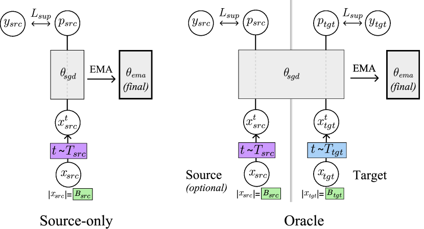
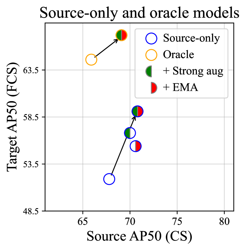
Figure 4: Revisiting source-only and oracle models in DAOD. We argue that in order to provide a fair measure of domain adaptation performance in DAOD, source-only and oracle models must utilize the same non-adaptive architectural and training components as methods being studied. In the case of Align and Distill-based approaches, this means source-only and oracle models must have access to the same set of source augmentations and EMA as DAOD methods. We see that these upgrades significantly improve source-only performance on target-domain data (+7.2 AP50 on Foggy Cityscapes), even though the source-only model has never seen any target-domain data, and these upgrades also improve oracle performance. Overall, these results set more challenging and realistic performance targets for DAOD methods.

Revisiting source-only and oracle models. Here we address P1: Improperly constructed source-only and oracle models, leading to overestimation of performance gains. The goal of DAOD is to develop adaptation techniques that use unlabeled target-domain data to improve target-domain performance. Thus, in order to properly isolate adaptation-specific techniques, any technique that does not need target-domain data to run should also be used by source-only and oracle models. In our case, this means that source-only and oracle models should also utilize the same strong augmentations and EMA updates as DAOD methods. In Fig. 4 we illustrate the resulting source-only and oracle models, and show that including these components significantly improves both source-only and oracle model performance (+7.2 and +2.6 AP50 on Foggy Cityscapes, respectively). This has significant implications for DAOD research: because source-only and oracle models have not been constructed with equivalent components, performance gains stemming from better generalization have until now been misattributed to DAOD. With properly constructed source-only and oracle models, the gains from DAOD are much more modest (see Fig. 5).

Modernizing architectures. We next address P3: (b) Outdated model architectures leading to overestimation of methods’ generality. Prior art in DAOD has used older backbones (e.g. VGG-16) in order to compare to previously-published results. To investigate whether conclusions drawn from these results generalize to modern experimental settings, our experiments utilize a modern detection framework [54] with default settings including multi-scale input transforms and COCO pre-training. We use a ResNet-50 backbone [23] with Feature Pyramid Network [35] and ViTDet [33]. We provide more details in the supplementary. Source-only and oracle models also receive these upgrades.

6.2 Fair Comparison and State-of-the-Art Results

We compare ALDI++ with reimplementations of five state-of-the-art DAOD methods on top of our framework: UMT [12], SADA [10], PT [8], MIC [26], and AT [34]; see Tab. 1 for the ALDI settings used to reproduce them. We use the fair benchmarking protocol proposed in Sec. 6.1. Results are shown in Fig. 5. All methods (including ALDI++) use the same settings for all benchmarks.

ALDI++ is state-of-the-art on CS $\rightarrow$ FCS, Sim10k $\rightarrow$ CS, and CFC Kenai $\rightarrow$ Channel. ALDI++ outperforms the previous state-of-the-art by +3.5 AP50 on CS $\rightarrow$ FCS, +5.7 AP50 on Sim10k $\rightarrow$ CS (where ours is the only method to outperform a fair source-only model), and +2.0 AP50 on CFC Kenai $\rightarrow$ Channel. Further, we achieve near-oracle level performance on CS $\rightarrow$ FCS and CFC Kenai $\rightarrow$ Channel (0.4 and 0.9 AP50 away, respectively), while other methods close less than half the gap between source-only and oracle models.

Modern architectures and fair source-only models create a paradigm shift for DAOD benchmarking. Our benchmarking protocol provides a dramatic reset for DAOD performance bounds. A fair and modern source-only model—trained without ever seeing any target domain data—achieves a higher target AP50 than all previously-published DAOD methods (see Fig. 1). Similarly, we see a 57% increase in oracle performance compared to prior work.

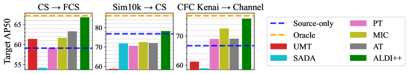
Figure 5: ALDI++ outperforms all prior work on CS $\rightarrow$ FCS, Sim10k $\rightarrow$ CS, and CFC Kenai $\rightarrow$ Channel. We provide a fair comparison of ALDI++ with five existing state-of-the-art approaches by upgrading them to use the ALDI framework. We see that some prior methods continue to provide benefit on top of a modern architecture but others lag behind modern source-only models. Our method ALDI++ outperforms prior work on all datasets studied by a significant margin: +3.5 AP50 on CS $\rightarrow$ FCS, +5.7 AP50 on Sim10k $\rightarrow$ CS, and +2.0 AP50 on CFC Kenai $\rightarrow$ Channel. Notably, ALDI++ is the only method to outperform a source-only model on Sim10k $\rightarrow$ CS.

Relative performance of all methods decreases compared to fair source-only and oracle models. Re-implementing SOTA methods in ALDI improves absolute performance of all methods; however performance decreases compared to source-only models. There are several instances where modernized DAOD methods are actually worse than a fair source-only model. Notably, a source-only model outperforms upgraded versions all previously-published work on Sim10 $\rightarrow$ CS. We also see that no state-of-the-art methods outperform a fair oracle on any dataset, in contrast to claims made by prior work [34, 8, 5].

The ranking of methods differs across datasets and architectures. MIC and AT are consistently the top-performing methods across all datasets. UMT exhibits variable performance due to the differences in the difficulty of image generation across datasets (see supplemental for examples). SADA underperforms other methods on CS $\rightarrow$ FCS and CFC Kenai $\rightarrow$ Channel, but closes this gap on the more difficult Sim10k $\rightarrow$ CS. These differences highlight the importance of benchmarking in a modern context, as we see that previously-published methods are not always complementary to general advancements in object detection. These results also demonstrate the utility of CFC-DAOD as another point of comparison for DAOD methods.

ALDI++ is compatible with new detector variants. We upgrade ALDI++ to use VitDet [33]. Since VitDet is a two-stage architecture based on Faster R-CNN, this requires no modifications to our multi-task distillation loss. We show that ALDI++ continue to show improvements over an upgraded VitDet source-only model (see Fig. 1 for CS $\rightarrow$ FCS and supplemental for other datasets). We see there is a larger gap between the ViT ALDI++ and the ViT oracle, indicating the potential for future work to improve performance.

6.3 Ablation Studies

In this section we ablate the performance of each component of ALDI on CS $\rightarrow$ FCS. For each ablation, unless otherwise specified we begin with the settings shown in Tab. 2, ablating one column at a time. Our default burn-in uses the same augmentations as the Fixed strategy from Tab. 1 but uses early stopping for model selection, and all self-training runs are initialized with the same burned-in checkpoint for fair comparison. See Tab. 1 for additional definitions.

Table 2: Starting point for all ablation experiments.

Method	$\theta_{stu},\theta_{tch}$ (Burn-in)	$T_{src}$	$T_{tgt}$	$\frac{B_{tgt}}{B}$	Postprocess	$L_{distill}$	$L_{align}$
Ablation start	Weak augs, early stopping	F, M	F, M, J, C	0.5	Thresh, NMS	Hard	–

$\theta_{stu}$, $\theta_{tch}$ Network initialization (burn-in). In Fig. 6a we analyze the effects of our proposed burn-in strategy (see Sec. 4). We measure performance in terms of target-domain AP50 as well as convergence time, defined as the training time at which the model first exceeds 95% of its final target-domain performance. We compare our approach with: (1) No dataset-specific burn-in, i.e. starting with COCO weights, and (2) The approach used by past work—using a fixed burn-in duration, e.g. 10k iterations. We find that our method results in significant improvements in both training speed and accuracy, leading to upwards of 10% improvements in AP50 and reducing training time by a factor of 10 compared to training without burn-in.

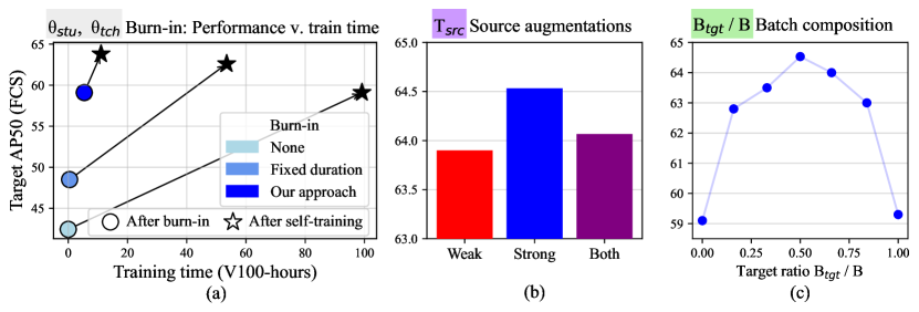
Figure 6: Ablating the components of ALDI++. (a) Our proposed burn-in strategy (Sec. 4) improves AP50_FCS by +4.7 and reduces training time by 10x compared to no burn-in. (b) Strong source-data augmentations during self-training lead to better performance. (c) An equal ratio of source and target data during self-training leads to best performance.

$T_{src}$ Source augmentations. In Fig. 6b we ablate the set of source-domain data augmentations. We compare using weak augmentations (random flipping and multi-scale training), strong augmentations (color jitter and random erasing), and a combination of weak and strong, noting that prior works differ in this regard but do not typically report the settings used (see Tab. 1). We find that using strong source augmentations on the entire source-domain training batch outperforms weak augmentations and a combination of both.

$T_{tgt}$ Target augmentations. In LABEL:tab:target_aug we investigate the use of different augmentations for target-domain inputs to the student model. (We note that weak augmentations are always used for target-domain inputs to the teacher in accordance with prior work). We see that stronger augmentations consistently improve performance, with best performance coming from the recently-proposed MIC augmentation [26].

Table 3: (a) Effects of target-domain augmentation on self-training. Augmentations applied to student inputs ($T_{tgt}$ in Fig. 2). Stronger augmentations improve performance considerably. (b) Effects of distillation objectives on self-training. We compare hard targets—used by most prior art, which thresholds teacher predictions to create pseudo-labels—with our proposed soft targets. Soft targets can improve overall performance. Results are the mean and 95% confidence intervals over 3 runs. (c) Feature alignment has diminishing returns. Alignment objectives $L_{align}$ without self-training provides up to 2.6 AP50 of benefit (left column), but diminishes to 0.2 AP50 additional gain when used alongside self-training (right column).

$T_{tgt}$	AP50FCS
Source-only model	51.9
Weak (scale & flip)	52.6
+ Color jitter	59.0
+ Color jitter + Erase	63.1
+ Color jitter + MIC	64.3

(a)

$L_{distill}$	AP50FCS
Source-only	59.1
Hard targets	63.7 $\pm$ 0.1
Soft targets	64.0 $\pm$ 0.4

(b)

$L_{align}$	$L_{distill}$	AP50FCS
Source-only		59.1
✓		61.7 (+2.6)
	✓	63.7 (+4.6)
✓	✓	63.9 (+4.8)

(c)

$B_{tgt}/B$ Batch composition. In Fig. 6c we ablate the ratio of source and target data within a minibatch. We note that prior works differ in this setting (see Tab. 1), but do not typically report what ratio is used. We see that using equal amounts of source and target data within each minibatch leads to the best performance. Notably, we also find that the inclusion of source-domain imagery is essential to see benefits from self-training—without any source imagery, AP50_FCS drops from 64.5 to 59.3.

$L_{distill}$ Self-distillation. In LABEL:tab:distill_ablate we analyze the effects of our proposed multi-task soft distillation approach (see Sec. 4). Note that for these experiments, the starting model is ALDI++ rather than the simple model in Tab. 2. We compare our approach with the “hard” pseudo-label approach used by prior work, where teacher predictions are post-processed with non-maximum suppression and a hard confidence threshold of 0.8 [26, 34, 12, 37]. For our proposed “soft” distillation method, we first sharpen teacher predictions at both detector stages using a sigmoid for objectness predictions and a softmax for classification predictions, both with a default temperature of 1. We see that our proposed soft targets improve performance compared to hard targets.

$L_{align}$ Feature alignment. Finally we investigate the use of feature alignment. We implement an adversarial feature alignment approach consisting of an image-level and instance-level feature discriminator (our implementation performs on par with SADA while being simpler to train; see supplemental material). In LABEL:tab:align, we show that feature alignment used in isolation (i.e. without self-training) offers performance gains up to 2.6 AP50. However, these performance gains are smaller than those seen from self-training (AP50_FCS of 61.7 vs. 63.1, respectively). When used in combination with self-training techniques, the additional benefit of feature alignment drops to $\leq$ 0.2 AP50_FCS. This suggests that self-training is currently the most promising avenue for progress and that more research is needed to develop complementary approaches. We also note that feature alignment approaches introduce training instability that may not be worth the small performance gain for practical use.

7 Discussion and Conclusions

In this work we proposed the ALDI framework and an improved DAOD benchmarking methodology, providing a critical reset for the DAOD research community; a new dataset CFC-DAOD, increasing the diversity and real-world applicability of DAOD benchmarks; and a new method ALDI++ that advances the state-of-the-art. We conclude with key findings.

Network initialization has an outsized impact. We find that general advancements in computer vision eclipse progress in DAOD: a Resnet50-FPN source-only model outperforms all VGG-based DAOD methods, and a VitDet source-only model outperforms all Resnet50-FPN based DAOD methods. Similarly, simply adding stronger augmentations and EMA to source-only models leads to better target-domain performance than some adaptation methods, and including these upgrades during network initialization (burn-in) improves adaptation performance as well.

DAOD techniques are helpful, but do not achieve oracle-level performance as previously claimed [34, 8, 5]. Top-performing DAOD methods, including ALDI++, demonstrate improvements over source-only models (see Fig. 1 and Fig. 5). However, in contrast to previously-published results, no DAOD method reaches oracle-level performance, suggesting there is still room for improvement. The gap between DAOD methods and oracles is even larger for stronger architectures like VitDet. This is a promising area for future research.

Benchmarks sourced from real-world domain adaptation challenges can help the community develop generally useful methods. We find that DAOD methods do not necessarily perform equivalently across datasets (see Fig. 5). Diverse benchmarks are useful to make sure we are not overfitting to the challenges of one particular use case, while exposing and supporting progress in impactful applications. Our contributed codebase and benchmark dataset provide the necessary starting point to enable this effort.

A lack of transparent comparisons has incentivized incremental progress in DAOD. Most highly-performant prior works in DAOD are some combination of DANN [17] (2016) and Mean Teacher [50] (2017) plus custom training techniques. Without fair comparisons it has been possible to propose near-duplicate methods that still achieve “state-of-the-art” performance due to hyperparameter tweaks. Our method ALDI++ establishes a strong point of comparison for Align and Distill-based approaches that will require algorithmic innovation to surpass.

Validation is the elephant in the room. All of our experiments, and all previously published work in DAOD, utilize a target-domain validation set to perform model and hyperparameter selection. This violates a key assumption in unsupervised domain adaptation: that no target-domain labels are available to begin with. Prior work has shown that it may not be possible to achieve performance improvements in domain adaptation at all under realistic validation conditions [38, 39, 31]. Therefore our results (as well as previously-published work) can really only be seen as an upper bound on DAOD performance. While this is valuable, further research is needed to develop effective unsupervised validation procedures for DAOD.

Acknowledgements. This material is based upon work supported by: NSF CISE Graduate Fellowships Grant #2313998, MIT EECS department fellowship #4000184939, MIT J-WAFS seed grant #2040131, and Caltech Resnick Sustainability Institute Impact Grant “Continuous, accurate and cost-effective counting of migrating salmon for conservation and fishery management in the Pacific Northwest.” Any opinions, findings, and conclusions or recommendations expressed in this material are those of the authors and do not necessarily reflect the views of NSF, MIT, J-WAFS, Caltech, or RSI. The authors acknowledge the MIT SuperCloud and Lincoln Laboratory Supercomputing Center for providing HPC resources [45]. We also thank the Alaska Department of Fish and Game for their ongoing collaboration and for providing data, and Sam Heinrich, Neha Hulkund, Kai Van Brunt, and Rangel Daroya for helpful feedback.

Align and Distill: Supplemental Material

Justin KayCorrespondence to: kayj@mit.edu Timm Haucke Suzanne Stathatos Siqi DengWork done outside AWS Erik Young Pietro Perona Sara BeeryEqual contribution Grant Van Horn

8 Additional Experiments

8.1 Adversarial Feature Alignment

We report additional ablations for the adversarial feature alignment network(s) used, comparing our implementations of image-level alignment and instance-level alignment with a baseline and SADA. As we see in LABEL:tab:alignment, LABEL:tab:alignment_sim10k, and LABEL:tab:alignment_cfc, the best settings to use differ by dataset. By default our feature alignment experiments in Sec. 6.1 of the main paper use both instance and image level alignment. See Sec. 9.4 below for further implementation details.

Table 4: Comparison of adversarial alignment methods. (a) Cityscapes $\rightarrow$ Foggy Cityscapes. We see that our implementations outperform SADA [10] while being simpler. Image-level alignment is best, followed by Image + Instance. (b) Sim10k $\rightarrow$ Cityscapes. Instance-level alignment is best. (c) CFC Kenai $\rightarrow$ Channel. Image + Instance is best. We see there is no consistently-best strategy across datasets; however, we note that for all datasets, the benefit of using adversarial feature alignment is smaller than self-training (see Sec. 6.3 of the main paper).

Method	AP50FCS
Baseline	51.9
SADA	54.2
Image-level (ours)	55.8
Instance-level (ours)	54.3
Image + Instance (ours)	54.9

(d)

Method	AP50CS
Baseline	70.8
Image-level (ours)	71.8
Instance-level (ours)	73.3
Image + Instance (ours)	71.5

(e)

Method	AP50Channel
Baseline	65.8
Image-level (ours)	65.2
Instance-level (ours)	66.0
Image + Instance (ours)	66.9

(f)

8.2 Visualizing Alignment

We investigate the overlap of source and target data in the feature space of different methods. For each method, we pool the highest-level feature maps of the backbone, either globally (“image-level”) or per instance (“instance-level”). We then embed the pooled feature vectors in 2D space using PCA for visual inspection (see Fig 7). We also compute a dissimilarity score based on FID [24], by fitting Gaussians to the source and target features and then computing the Fréchet distance between them.

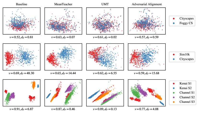
Figure 7: Embedding of pooled features from the final backbone layer in 2D space using PCA for four different methods. The ratio of variance explained by the first two PCA components is given by $v$ and a dissimilarity score between source and target features is given by $d_{F}$. $d_{F}$ is lower than the baseline for all alignment methods and does roughly match the overall visual trend in feature overlap. In all cases, the simple MeanTeacher model significantly reduces the distance between source and target data even though there is no explicit alignment criterion, even resulting in a smaller $d_{F}$ than adversarial alignment methods for CS $\rightarrow$ FCS & CFC Kenai $\rightarrow$ Channel.

8.3 ViT backbones

Table 5: ViT backbone results for: (a) Sim10k $\rightarrow$ Cityscape and (b) CFC Kenai $\rightarrow$ Channel.

Method	AP50CS
ViT baseline	81.7
ALDI++ + ViT	81.8
ViT oracle	89.8

(a)

Method	AP50Channel
ViT baseline	69.0
ALDI++ + ViT	71.1
ViT oracle	76.7

(b)

We show results using ALDI++ in combination with VitDet [33] in LABEL:tab:vit1 (Sim10k $\rightarrow$ Cityscapes) and LABEL:tab:vit2 (CFC Kenai $\rightarrow$ Channel). We see that ALDI continues to demonstrate improvements over baselines even as overall architectures get stronger, those these improvements are smaller in magnitude as also reported in the main paper Sec. 6.3 (CS $\rightarrow$ FCS results).

8.4 Teacher update

Table 6: Comparison of teacher update approaches on Cityscapes $\rightarrow$ Foggy Cityscapes. Mean teacher greatly outperforms other options.

Method	AP50FCS
Baseline	51.9
No update (vanilla self-training)	52.9
Student is teacher	53.8
EMA (mean teacher)	63.5

We compare other approaches to updating the teacher during self-training vs. using exponential moving average in Tab. 6. We see that EMA significantly outperforms using a fixed teacher (i.e. vanilla self-training, where pseudo-labels are generated once before training) as well as using the student as its own teacher without EMA.

8.5 Example of (Un)Fair Comparisons

In Fig. 8 we show a case study of why fair comparisons are impactful for DAOD research. We compare two similarly-performing prior works, AT and MIC, and see that implementation inconsistencies have led to nontransparent comparisons between the two methods. Notably, the originally reported results even used different ground truth test labels. When re-implemented on top of the same modern framework using ALDI, we are able to fairly compare the two methods for the first time.

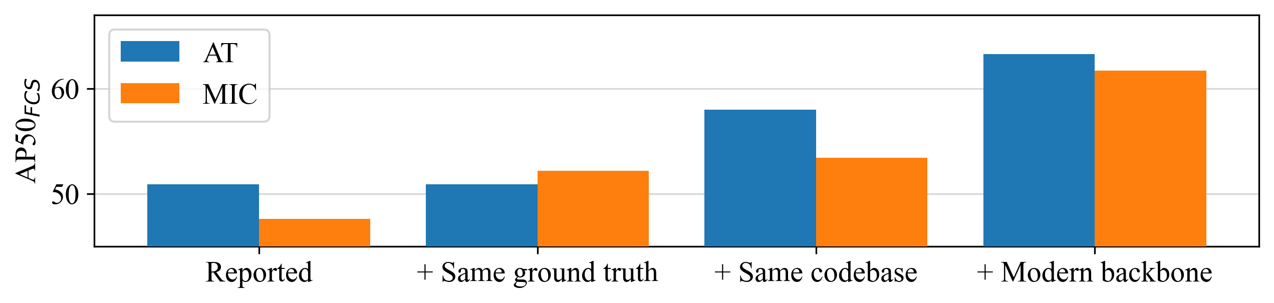
Figure 8: Effects of fair and modernized comparison between MIC and AT. Here we show an example of why fair and modern comparisons are necessary for making principled progress in DAOD. Moving left to right: (1) Published results report a difference of 3.3 AP50 on Cityscapes $\rightarrow$ Foggy Cityscapes between the two methods; (2) However the authors used different truth test labels, and when this is corrected we see that the originally-published MIC model actually outperforms the originally-published AT model; (3) The authors also used different object detection libraries (Detectron2 for AT and maskrcnn-benchmark for MIC); when we re-implement them on top of ALDI (still using the VGG-16 backbones proposed in the original papers), we see that AT significantly outperforms MIC, but (4) These performance diferences are less pronounced when using a modern backbone, indicating that for practical use there is less difference between these two methods than previously reported.

9 Implementation Details

9.1 Re-implementations of Other Methods

Here we include additional details regarding our re-implementations of prior work on top of the ALDI framework. We visualize our implementations in Fig. 9.

9.1.1 Adaptive Teacher [34]

Adaptive Teacher (AT) uses the default settings from the base configuration in Table 2 of the main paper, plus an image-level alignment network. For fair reproduction, we used the authors’ alignment network implementation instead of our own for all AT experiments.

9.1.2 MIC [26]

We reimplemented the masked image consistency augmentation as a Detectron2 Transform in our framework for efficiency. We also implemented MIC’s “quality weight” loss re-weighting procedure, though in our experiments we found that it makes performance slightly worse (AP50 on Foggy Cityscapes of 62.8 vs. 63.1 without).

9.1.3 Probabilistic Teacher [8]

Probabilistic Teacher (PT) utilizes: (1) a custom Faster R-CNN architecture that makes localization predictions probabilistic, called “Gaussian R-CNN”, (2) a focal loss objective, (3) learnable anchors. We ported implementations of these three components to our framework. Note that we first had to burn in a Gaussian R-CNN, so PT was not able to use the exact same starting weights as other methods.

9.1.4 SADA [10]

We port the official implementation of SADA to Detectron2. Note that SADA does not include burn-in or self-training, so the base implementation is the Detectron2 baseline config.

9.1.5 Unbiased Mean Teacher [12]

Our implementation mirrors the UMT_SCA configuration from  [12].

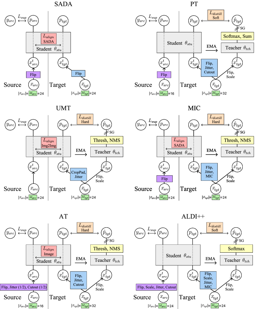
Figure 9: Visual depiction of ALDI settings for reproducing prior work.

9.2 Faster R-CNN Losses

Here we describe the standard Faster R-CNN losses before describing how we modify them into “soft” distillation losses. Faster R-CNN consists of two stages: a region proposal network and the region-of-interest heads.

9.2.1 Region proposal network (RPN):

Inputs. The RPN takes as input:

1. Features extracted by a backbone network (e.g. a Resnet-50 with feature pyramid network in most of our experiments).

2. A set of anchor boxes that represent the initial candidates for detection.

Outputs. For each anchor, the RPN predicts two things:

1. A binary classification called “objectness” representing whether the content inside the anchor box is foreground or background.

2. Regression targets for the anchor, representing adjustments to the box to more closely enclose any foreground objects.

Computing the loss. In order to evaluate these predicted proposals, each proposal is matched to either foreground or background based on its intersection-over-union with the nearest ground truth box. Based on these matches, in the Detectron2 default settings a binary cross-entropy loss is computed for (1) and a smooth L1 loss is computed for (2).

A key challenge in Faster R-CNN is the severe imbalance between foreground and background anchors. To address this, a smaller number of proposals are sampled for computing the loss (256 in the default settings) with a specified foreground ratio (0.5 in the default setting). Objectness loss is computed for all proposals, while the box regression loss is computed only for foreground proposals (since it is undefined how the network should regress background proposals).

9.2.2 Region of interest (ROI) heads:

Inputs. The ROI heads take as input:

1. Proposals from the RPN. In training, these are sampled at a desired foreground/background ratio, similar to the procedure used for computing the loss in the RPN. Note, however, that these will be different proposals than those used to compute RPN loss. In the Detectron2 defaults, 512 RPN proposals are sampled as inputs to the ROI heads at a foreground ratio of 0.25.

2. Cropped backbone features, extracted using a procedure such as ROIAlign [22]. These are the features in the backbone feature map that are “inside” each proposal.

Outputs. The ROI heads then predict for each proposal:

1. A multi-class classification.

2. Regression targets for the final bounding box, representing adjustments to the box to more closely enclose any foreground objects.

Computing the loss. Predicted boxes are matched with ground truth boxes again based on intersection-over-union in order to compute the loss. By default we compute a cross-entropy loss for (1) and a smooth L1 loss for (2). (2) is again only computed for foreground predictions.

9.3 Soft Distillation Losses for Faster R-CNN

Distillation losses are computed between teacher predictions and student predictions. One option is select the teacher’s most confident predictions based on a confidence threshold parameter to be “pseudo-labels.” These take the place of ground truth boxes in the standard Faster R-CNN losses for the student. We refer to this approach as using “hard targets.”

In contrast, here we describe how we compute “soft” losses using intermediate outputs from the teacher to guide the student without thresholding.

RPN. The teacher and student RPNs start with the same anchors. We use the same sampling procedure described in 9.2.1 for choosing proposals for loss computation. Importantly, we ensure the same proposals are sampled from the teacher and student so that they can be directly compared. We postprocess the teacher’s objectness predictions with a sigmoid function to sharpen them. We then compute a binary cross-entropy loss between the teacher’s post-sigmoid outputs and student’s objectness predictions. We also compute a smooth L1 loss between the teacher’s RPN regression predictions and the student’s RPN regression predictions. Regression losses are only computed on proposals where the teacher’s post-sigmoid objectness score is $\geq$ 0.8.

ROI heads. The second stage of Faster R-CNN predicts a classification and regression for each RPN proposal; therefore, we need the input proposals to the student and teacher to be the same in order to directly compare their outputs. To achieve this, during soft distillation we initialize the student and teacher’s ROI heads with the student’s RPN proposals—intuitively, we want the teacher to tell the student “what to do with” its proposals from the first stage.

We postprocess the teacher’s classification predictions with a softmax to sharpen them, then compute a cross-entropy loss between the teacher’s post-softmax predictions and the student’s classification predictions. We also compute a smooth L1 loss between the teacher’s regression predictions and the student’s regression predictions. We only compute regression losses where the teacher’s top-scoring class prediction is not the background class.

9.4 Adversarial Feature Alignment

We implement two networks to perform adversarial alignment at the image level and instance (bounding box) level. Our approach is inspired by Faster R-CNN in the Wild [9] and SADA [10].

Image-level alignment. We build an adversarial discriminator network that takes in backbone features at the image level. By default we use the “p2” layer of the feature pyramid network as described in [35]. We use a simple convolutional head consisting of one hidden layer. Our defaults result in this torch module:

ConvDiscriminator(
    (model): Sequential(
      (0): Conv2d(256, 256,
                    kernel_size=(3, 3),
                    stride=(1, 1))
      (1): ReLU()
      (2): AdaptiveAvgPool2d(output_size=1)
      (3): Flatten(start_dim=1, end_dim=-1)
      (4): Linear(in_features=256,
                    out_features=1,
                    bias=True)
    )
  )

Instance-level alignment. We also implement an instance-level adversarial alignment network that takes as input the penultimate layer of the ROI heads classification head. By default, our instance level discriminator consists of one hidden fully-connected layer. Our defaults result in this torch module:

FCDiscriminator(
    (model): Sequential(
      (0): Flatten(start_dim=1, end_dim=-1)
      (1): Linear(in_features=1024,
                    out_features=1024,
                    bias=True)
      (2): ReLU()
      (3): Linear(in_features=1024,
                    out_features=1,
                    bias=True)
    )
)

10 Experiment Details

10.1 Backbone Pretraining

In our experiments, we evaluate two different backbones: a ResNet-50 [23] with Feature Pyramid Network [35], and a ViT-B [14] with ViTDet [33]. Both backbones are pre-trained on the ImageNet-1K classification and the COCO instance segmentation [36] tasks. In addition, the ViT-B backbone is also pre-trained using the masked autoencoder objective proposed in [20].

10.2 Image-to-Image Translation

In contrast to the adversarial alignment in feature space as in SADA [10], UMT [12] aligns the domains in image (i.e. pixel) space. This is achieved by training and using an unpaired image-to-image translation model to try to transform images from the source dataset into images that look like images from the target dataset (“target-like”) and vice-versa (“source-like”). We follow [12] by using the CycleGAN [56] image-to-image translation model. We train the CycleGAN for 200 epochs (Cityscapes $\leftrightarrow$ Foggy Cityscapes, Sim10k $\leftrightarrow$ CS) or 20 epochs (Kenai $\leftrightarrow$ Channel) and respectively select the best model according to the average Fréchet inception distance (FID) [24] between the source & source-like and the target & target-like images in the training dataset. For FID computation, we use the clean-fid implementation proposed in [42]. We compute FID on the training datasets as UMT only uses translated images thereof, which is why we are only interested in the best fit on the training data. We follow [12] by then generating source-like and target-like dataset using the selected model ahead of time, before the training of the main domain adaptation method. We note that tuning CycleGAN’s hyperparameters or using other image-to-image translation methods could possibly improve UMT’s performance however for the fair reproduction we use the defaults. We show some exemplary results of our CycleGAN models that are used to train UMT [12] in Fig 10.

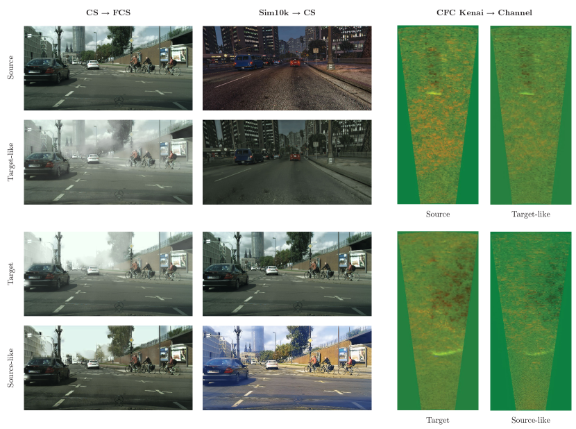
Figure 10: Exemplary results of our CycleGAN models. Source and target are the original images. Target-like and source-like are images translated by CycleGAN. Since FCS is derived from CS, CS $\rightarrow$ FCS is the only case in which we have paired images and can therefore show the translation from source into target-like and from target into source-like for the same example.

10.3 Other Training Settings

We fix the total effective batch size at 48 samples for fair comparison across all experiments. For training, we perform each experiments on 8 Nvidia V100 (32GB) GPUs distributed over four nodes. We use the MIT Supercloud [45].

11 CFC-DAOD Dataset Details

Like other DAOD benchmarks, CFC-DAOD consists of data from two domains, source and target.

11.1 Source data

Train: In CFC-DAOD, the source-domain training set consists of training data from the original CFC data release, i.e., video frames from the “Kenai left bank” location. We have used the 3-channel “Baseline++” format introduced in the original CFC paper [30]. For experiments in the ALDI paper, we subsampled empty frames to be around 10% of the total data, resulting in 76,619 training images. For reproducibility, we release the exact subsampled set. When publishing results on CFC-DAOD, however, researchers are allowed to use the orignial CFC training set however they see fit and are not required to use our subsampled “Baseline++” data.

Validation: The CFC-DAOD Kenai (source) validation set is the same as the original CFC validation set. We use the 3-channel “Baseline++” format from the original CFC paper. There are 30,454 validation images.

11.2 Target data

Train: In CFC-DAOD, the target-domain “training” set consists of new data from the “Kenai Channel” location in CFC. These frames should be treated as unlabeled for DAOD methods, but labeled for Oracle methods. We also use the “Baseline++” format, and use the authors’ original code for generating the image files from the original video files for consistency. There are 29,089 target train images.

Test: The CFC-DAOD target-domain test set is the same as the “Kenai Channel” test set from CFC. We use the “Baseline++” format. There are 13,091 target test images. Researchers should publish final mAP@Iou=0.5 numbers on this data, and may use this data for model selection for fair comparison with prior methods.

12 The ALDI Codebase

We release ALDI as an open-source codebase built on a modern detector implementation. The codebase is optimized for speed, accuracy, and extensibility, training up to 5x faster than existing DAOD codebases while requiring up to 13x fewer lines of code. These qualities make our framework valuable for practitioners developing detection models in real applications, as well as for researchers pushing the state-of-the-art in DAOD.

Table 7: Open-source codebases in domain adaptive object detection. Existing methods use a variety of different detector implementations, including deprecated frameworks (maskrcnn-benchmark) and versions (Detectron2 $<$ v0.6). In contrast, ALDI is built on top of a modern framework, optimized for training speed, and is able to reproduce all five of these methods while requiring fewer lines of code (LOC) than any individual existing implementation. Our codebase can serve as a strong starting point for future research.

Codebase	Faster R-CNN	LOC
	Implementation
UMT [12]	faster-rcnn.pytorch	19k
SADA [10]	maskrcnn-benchmark	7k
PT [8]	Detectron2 v0.5	3.4k
MIC [26]	maskrcnn-benchmark	20k
AT [34]	Detectron2 v0.3	4k
ALDI (Ours)	Detectron2 $\sim$v0.7	1.5k

12.1 Detection Framework

We designed the ALDI codebase to be lightweight and extensible. For this reason, we build on top of a recent version of Detectron2 [54]. The last tagged release of Detectron2 was v0.6 in November 2021, however there have been a number upgrades since then leading to state-of-the-art performance. Thus, we use a fixed version that we call v0.7ish based off of an unofficial pull request for v0.7, commit 7755101 dated August 30 2023. We include this version of Detectron2 as a pip-installable submodule in the ALDI codebase for now, noting that once the official version is released it will no longer need to be a submodule (i.e. it will be able to be directly installed through pip without cloning any code).

Our codebase makes no modifications to the underlying Detectron2 code, making it a lightweight standalone framework. This is in contrast to existing DAOD codebases (see Tab. 7) that often duplicate and modify the underlying framework as part of their implementation. By building on top of Detectron2 rather than within it, our codebase is up to 13x smaller than other DAOD codebases while providing more functionality. We note that in Tab. 7, other codebases implement a single method while ours supports all methods studied.

12.2 Speedups

We found significant bottlenecks in training in other Detectron2-based codebases. Notably, we found that dataloaders and transform implementations were inefficient. These included, for instance:

• Converting tensors back and forth between torch, numpy, and PIL during augmentation. We addressed this, reimplementing transforms as needed so that everything stays in torch.

• Using the random hue transform from torchvision. We found minimal changes in performance from disabling this component of the ColorJitter transform.

• Using separate dataloaders for weakly and strongly augmented imagery. We instead use a single dataloader per domain, with a hook to retrieve weakly augmented imagery before strong augmentations are performed.

We reimplemented the dataloaders and augmentation strategies used by AT, MIC, and others to be more efficient, leading to a 5x speedup in training time per image compared to AT.

References

- [1] Anonymous: Exponential moving average of weights in deep learning: Dynamics and benefits. Submitted to Transactions on Machine Learning Research (2023), https://openreview.net/forum?id=2M9CUnYnBA, under review
- [2] Arpit, D., Wang, H., Zhou, Y., Xiong, C.: Ensemble of averages: Improving model selection and boosting performance in domain generalization. Advances in Neural Information Processing Systems 35, 8265–8277 (2022)
- [3] Bondi, E., Fang, F., Hamilton, M., Kar, D., Dmello, D., Choi, J., Hannaford, R., Iyer, A., Joppa, L., Tambe, M., et al.: Spot poachers in action: Augmenting conservation drones with automatic detection in near real time. In: Proceedings of the AAAI Conference on Artificial Intelligence. vol. 32 (2018)
- [4] Cai, Q., Pan, Y., Ngo, C.W., Tian, X., Duan, L., Yao, T.: Exploring object relation in mean teacher for cross-domain detection. In: Proceedings of the IEEE/CVF Conference on Computer Vision and Pattern Recognition. pp. 11457–11466 (2019)
- [5] Cao, S., Joshi, D., Gui, L.Y., Wang, Y.X.: Contrastive mean teacher for domain adaptive object detectors. In: Proceedings of the IEEE/CVF Conference on Computer Vision and Pattern Recognition. pp. 23839–23848 (2023)
- [6] Caron, M., Touvron, H., Misra, I., Jégou, H., Mairal, J., Bojanowski, P., Joulin, A.: Emerging properties in self-supervised vision transformers. In: Proceedings of the IEEE/CVF international conference on computer vision. pp. 9650–9660 (2021)
- [7] Chen, G., Choi, W., Yu, X., Han, T., Chandraker, M.: Learning efficient object detection models with knowledge distillation. Advances in neural information processing systems 30 (2017)
- [8] Chen, M., Chen, W., Yang, S., Song, J., Wang, X., Zhang, L., Yan, Y., Qi, D., Zhuang, Y., Xie, D., et al.: Learning domain adaptive object detection with probabilistic teacher. arXiv preprint arXiv:2206.06293 (2022)
- [9] Chen, Y., Li, W., Sakaridis, C., Dai, D., Van Gool, L.: Domain adaptive faster r-cnn for object detection in the wild. In: Proceedings of the IEEE conference on computer vision and pattern recognition. pp. 3339–3348 (2018)
- [10] Chen, Y., Wang, H., Li, W., Sakaridis, C., Dai, D., Van Gool, L.: Scale-aware domain adaptive faster r-cnn. International Journal of Computer Vision 129(7), 2223–2243 (2021)
- [11] Cordts, M., Omran, M., Ramos, S., Rehfeld, T., Enzweiler, M., Benenson, R., Franke, U., Roth, S., Schiele, B.: The cityscapes dataset for semantic urban scene understanding. In: Proceedings of the IEEE conference on computer vision and pattern recognition. pp. 3213–3223 (2016)
- [12] Deng, J., Li, W., Chen, Y., Duan, L.: Unbiased mean teacher for cross-domain object detection. In: Proceedings of the IEEE/CVF Conference on Computer Vision and Pattern Recognition. pp. 4091–4101 (2021)
- [13] DeVries, T., Taylor, G.W.: Improved regularization of convolutional neural networks with cutout. arXiv preprint arXiv:1708.04552 (2017)
- [14] Dosovitskiy, A., Beyer, L., Kolesnikov, A., Weissenborn, D., Zhai, X., Unterthiner, T., Dehghani, M., Minderer, M., Heigold, G., Gelly, S., et al.: An image is worth 16x16 words: Transformers for image recognition at scale. arXiv preprint arXiv:2010.11929 (2020)
- [15] Everingham, M., Van Gool, L., Williams, C.K., Winn, J., Zisserman, A.: The pascal visual object classes (voc) challenge. International journal of computer vision 88(2), 303–338 (2010)
- [16] Ganin, Y., Lempitsky, V.: Unsupervised domain adaptation by backpropagation. In: International conference on machine learning. pp. 1180–1189. PMLR (2015)
- [17] Ganin, Y., Ustinova, E., Ajakan, H., Germain, P., Larochelle, H., Laviolette, F., Marchand, M., Lempitsky, V.: Domain-adversarial training of neural networks. The journal of machine learning research 17(1), 2096–2030 (2016)
- [18] Gao, I., Sagawa, S., Koh, P.W., Hashimoto, T., Liang, P.: Out-of-distribution robustness via targeted augmentations. In: NeurIPS 2022 Workshop on Distribution Shifts: Connecting Methods and Applications (2022)
- [19] Guan, H., Liu, M.: Domain adaptation for medical image analysis: a survey. IEEE Transactions on Biomedical Engineering 69(3), 1173–1185 (2021)
- [20] He, K., Chen, X., Xie, S., Li, Y., Dollár, P., Girshick, R.: Masked autoencoders are scalable vision learners. In: Proceedings of the IEEE/CVF conference on computer vision and pattern recognition. pp. 16000–16009 (2022)
- [21] He, K., Fan, H., Wu, Y., Xie, S., Girshick, R.: Momentum contrast for unsupervised visual representation learning. In: Proceedings of the IEEE/CVF conference on computer vision and pattern recognition. pp. 9729–9738 (2020)
- [22] He, K., Gkioxari, G., Dollár, P., Girshick, R.: Mask r-cnn. In: Proceedings of the IEEE international conference on computer vision. pp. 2961–2969 (2017)
- [23] He, K., Zhang, X., Ren, S., Sun, J.: Deep residual learning for image recognition. In: Proceedings of the IEEE conference on computer vision and pattern recognition. pp. 770–778 (2016)
- [24] Heusel, M., Ramsauer, H., Unterthiner, T., Nessler, B., Hochreiter, S.: Gans trained by a two time-scale update rule converge to a local nash equilibrium. Advances in neural information processing systems 30 (2017)
- [25] Hinton, G., Vinyals, O., Dean, J.: Distilling the knowledge in a neural network. arXiv preprint arXiv:1503.02531 (2015)
- [26] Hoyer, L., Dai, D., Wang, H., Van Gool, L.: Mic: Masked image consistency for context-enhanced domain adaptation. In: Proceedings of the IEEE/CVF Conference on Computer Vision and Pattern Recognition. pp. 11721–11732 (2023)
- [27] Inoue, N., Furuta, R., Yamasaki, T., Aizawa, K.: Cross-domain weakly-supervised object detection through progressive domain adaptation. In: Proceedings of the IEEE conference on computer vision and pattern recognition. pp. 5001–5009 (2018)
- [28] Johnson-Roberson, M., Barto, C., Mehta, R., Sridhar, S.N., Rosaen, K., Vasudevan, R.: Driving in the matrix: Can virtual worlds replace human-generated annotations for real world tasks? arXiv preprint arXiv:1610.01983 (2016)
- [29] Kalluri, T., Xu, W., Chandraker, M.: Geonet: Benchmarking unsupervised adaptation across geographies. CVPR (2023)
- [30] Kay, J., Kulits, P., Stathatos, S., Deng, S., Young, E., Beery, S., Van Horn, G., Perona, P.: The caltech fish counting dataset: A benchmark for multiple-object tracking and counting. In: European Conference on Computer Vision. pp. 290–311. Springer (2022)
- [31] Kay, J., Stathatos, S., Deng, S., Young, E., Perona, P., Beery, S., Van Horn, G.: Unsupervised domain adaptation in the real world: A case study in sonar video. In: NeurIPS 2023 Computational Sustainability: Promises and Pitfalls from Theory to Deployment (2023)
- [32] Koh, P.W., Sagawa, S., Marklund, H., Xie, S.M., Zhang, M., Balsubramani, A., Hu, W., Yasunaga, M., Phillips, R.L., Gao, I., et al.: Wilds: A benchmark of in-the-wild distribution shifts. In: International Conference on Machine Learning. pp. 5637–5664. PMLR (2021)
- [33] Li, Y., Mao, H., Girshick, R., He, K.: Exploring plain vision transformer backbones for object detection. In: European Conference on Computer Vision. pp. 280–296. Springer (2022)
- [34] Li, Y.J., Dai, X., Ma, C.Y., Liu, Y.C., Chen, K., Wu, B., He, Z., Kitani, K., Vajda, P.: Cross-domain adaptive teacher for object detection. In: Proceedings of the IEEE/CVF Conference on Computer Vision and Pattern Recognition. pp. 7581–7590 (2022)
- [35] Lin, T.Y., Dollár, P., Girshick, R., He, K., Hariharan, B., Belongie, S.: Feature pyramid networks for object detection. In: Proceedings of the IEEE conference on computer vision and pattern recognition. pp. 2117–2125 (2017)
- [36] Lin, T.Y., Maire, M., Belongie, S., Hays, J., Perona, P., Ramanan, D., Dollár, P., Zitnick, C.L.: Microsoft coco: Common objects in context. In: European conference on computer vision. pp. 740–755. Springer (2014)
- [37] Liu, Y.C., Ma, C.Y., He, Z., Kuo, C.W., Chen, K., Zhang, P., Wu, B., Kira, Z., Vajda, P.: Unbiased teacher for semi-supervised object detection. arXiv preprint arXiv:2102.09480 (2021)
- [38] Musgrave, K., Belongie, S., Lim, S.N.: Unsupervised domain adaptation: A reality check. arXiv preprint arXiv:2111.15672 (2021)
- [39] Musgrave, K., Belongie, S., Lim, S.N.: Benchmarking validation methods for unsupervised domain adaptation. arXiv preprint arXiv:2208.07360 (2022)
- [40] Nguyen, D.K., Tseng, W.L., Shuai, H.H.: Domain-adaptive object detection via uncertainty-aware distribution alignment. In: Proceedings of the 28th ACM international conference on multimedia. pp. 2499–2507 (2020)
- [41] Oza, P., Sindagi, V.A., Sharmini, V.V., Patel, V.M.: Unsupervised domain adaptation of object detectors: A survey. IEEE Transactions on Pattern Analysis and Machine Intelligence (2023)
- [42] Parmar, G., Zhang, R., Zhu, J.Y.: On aliased resizing and surprising subtleties in gan evaluation. In: Proceedings of the IEEE/CVF Conference on Computer Vision and Pattern Recognition. pp. 11410–11420 (2022)
- [43] Pham, M., Cho, M., Joshi, A., Hegde, C.: Revisiting self-distillation. arXiv preprint arXiv:2206.08491 (2022)
- [44] Ren, S., He, K., Girshick, R., Sun, J.: Faster r-cnn: Towards real-time object detection with region proposal networks. Advances in neural information processing systems 28 (2015)
- [45] Reuther, A., Kepner, J., Byun, C., Samsi, S., Arcand, W., Bestor, D., Bergeron, B., Gadepally, V., Houle, M., Hubbell, M., Jones, M., Klein, A., Milechin, L., Mullen, J., Prout, A., Rosa, A., Yee, C., Michaleas, P.: Interactive supercomputing on 40,000 cores for machine learning and data analysis. In: 2018 IEEE High Performance extreme Computing Conference (HPEC). pp. 1–6. IEEE (2018)
- [46] Rodriguez, M., Laptev, I., Sivic, J., Audibert, J.Y.: Density-aware person detection and tracking in crowds. In: 2011 International Conference on Computer Vision. pp. 2423–2430. IEEE (2011)
- [47] Saito, K., Ushiku, Y., Harada, T., Saenko, K.: Strong-weak distribution alignment for adaptive object detection. In: Proceedings of the IEEE/CVF Conference on Computer Vision and Pattern Recognition. pp. 6956–6965 (2019)
- [48] Sakaridis, C., Dai, D., Van Gool, L.: Semantic foggy scene understanding with synthetic data. International Journal of Computer Vision 126, 973–992 (2018)
- [49] Schneider, S., Taylor, G.W., Kremer, S.: Deep learning object detection methods for ecological camera trap data. In: 2018 15th Conference on computer and robot vision (CRV). pp. 321–328. IEEE (2018)
- [50] Tarvainen, A., Valpola, H.: Mean teachers are better role models: Weight-averaged consistency targets improve semi-supervised deep learning results. Advances in neural information processing systems 30 (2017)
- [51] Vs, V., Gupta, V., Oza, P., Sindagi, V.A., Patel, V.M.: Mega-cda: Memory guided attention for category-aware unsupervised domain adaptive object detection. In: Proceedings of the IEEE/CVF Conference on Computer Vision and Pattern Recognition. pp. 4516–4526 (2021)
- [52] Weinstein, B.G., Gardner, L., Saccomanno, V., Steinkraus, A., Ortega, A., Brush, K., Yenni, G., McKellar, A.E., Converse, R., Lippitt, C., et al.: A general deep learning model for bird detection in high resolution airborne imagery. bioRxiv (2021)
- [53] Weinstein, B.G., Graves, S.J., Marconi, S., Singh, A., Zare, A., Stewart, D., Bohlman, S.A., White, E.P.: A benchmark dataset for canopy crown detection and delineation in co-registered airborne rgb, lidar and hyperspectral imagery from the national ecological observation network. PLoS computational biology 17(7), e1009180 (2021)
- [54] Wu, Y., Kirillov, A., Massa, F., Lo, W.Y., Girshick, R.: Detectron2. https://github.com/facebookresearch/detectron2 (2019)
- [55] Xue, Z., Yang, F., Rajaraman, S., Zamzmi, G., Antani, S.: Cross dataset analysis of domain shift in cxr lung region detection. Diagnostics 13(6), 1068 (2023)
- [56] Zhu, J.Y., Park, T., Isola, P., Efros, A.A.: Unpaired image-to-image translation using cycle-consistent adversarial networks. In: Proceedings of the IEEE international conference on computer vision. pp. 2223–2232 (2017)
- [57] Zhu, X., Pang, J., Yang, C., Shi, J., Lin, D.: Adapting object detectors via selective cross-domain alignment. In: Proceedings of the IEEE/CVF Conference on Computer Vision and Pattern Recognition. pp. 687–696 (2019)