A tweezer array with 6100 highly coherent atomic qubits

Abstract

Optical tweezer arrays have had a transformative impact on atomic and molecular physics over the past years, and they now form the backbone for a wide range of leading experiments in quantum computing, simulation, and metrology. Underlying this development is the simplicity of single particle control and detection inherent to the technique. Typical experiments trap tens to hundreds of atomic qubits, and very recently systems with around one thousand atoms were realized without defining qubits or demonstrating coherent control. However, scaling to thousands of atomic qubits with long coherence times and low-loss, high-fidelity imaging is an outstanding challenge and critical for progress in quantum computing, simulation, and metrology, in particular, towards applications with quantum error correction. Here, we experimentally realize an array of optical tweezers trapping over 6,100 neutral atoms in around 12,000 sites while simultaneously surpassing state-of-the-art performance for several key metrics associated with fundamental limitations of the platform. Specifically, while scaling to such a large number of atoms, we also demonstrate a coherence time of 12.6(1) seconds, a record for hyperfine qubits in an optical tweezer array. Further, we show trapping lifetimes close to 23 minutes in a room-temperature apparatus, enabling record-high imaging survival of $99.98952(1)\%$ in combination with an imaging fidelity of over $99.99\%$. Our results, together with other recent developments, indicate that universal quantum computing with ten thousand atomic qubits could be a near-term prospect. Furthermore, our work could pave the way for quantum simulation and metrology experiments with inherent single particle readout and positioning capabilities at a similar scale.

Optical tweezer arrays ^{browaeys_many-body_2020, kaufman_quantum_2021} have transformed atomic and molecular physics experiments by simplifying detection and enabling control at the individual-particle level ^{barredo_atom-by-atom_2016, endres_atom-by-atom_2016, kim_situ_2016, liu_building_2018, anderegg_optical_2019}, resulting in rapid, recent progress in quantum computing ^{saffman_quantum_2016, henriet_quantum_2020, bluvstein_quantum_2022, graham_multi-qubit_2022, ma_universal_2022, finkelstein_universal_2024}, quantum simulation ^{bernien_probing_2017, browaeys_many-body_2020, ebadi_quantum_2021, scholl_quantum_2021, shaw_benchmarking_2024}, and optical frequency metrology ^{norcia_seconds-scale_2019, madjarov_atomic-array_2019, young_half-minute-scale_2020}. They are part of broader efforts towards single atom control in optical traps, including lattices ^{miroshnychenko_atom-sorting_2006, weitenberg_single-spin_2011} and lattice-tweezer hybrid systems ^{young_half-minute-scale_2020, tao_high-fidelity_2023, gyger_continuous_2024}. For quantum computers, simulators of spin systems and tweezer clocks, each atom typically encodes a single qubit that is controlled with electromagnetic fields, and ideally features long coherence times to enable these applications with high fidelity. Such optically trapped atomic qubits coexist with other platforms that have single qubit control and readout, including ion traps ^{bruzewicz_trapped-ion_2019} and superconducting qubits ^{kjaergaard_superconducting_2020}.

There are important incentives to scale up such fully programmable qubit platforms. For example, optical clocks gain in stability with increasing atom number ^{ludlow_optical_2015, rosenband_exponential_2013}, and proposals have been made for quantum simulation experiments that benefit from several thousand qubits to explore emergent collective behavior ^{orourke_entanglement_2023, julia-farre_amorphous_2024} or to demonstrate verifiable quantum advantage ^{haferkamp_closing_2020, ringbauer_verifiable_2023}.

In particular, quantum error correction (QEC) requires large system sizes, while maintaining high fidelities and long coherence times, in order to scale up the number of logical qubits ^{preskill_quantum_2018, google_quantum_ai_suppressing_2023}. Even the most resource-efficient QEC protocols require at least several thousand physical qubits with an error-per-gate level of $10^{-3}$ to encode $>$100 error-corrected logical qubits ^{bravyi_high-threshold_2023, xu_constant-overhead_2023}. However, published results from universal quantum computing architectures based on ion traps and superconducting qubits currently leverage only tens to hundreds of qubits ^{moses_race_2023, kim_evidence_2023}, and with current technologies for fabrication and control, generally suffer from deleterious effects as they are scaled ^{kjaergaard_superconducting_2020, bruzewicz_trapped-ion_2019}.

Neutral atoms in optical tweezer arrays are a promising platform towards rapid scalability in the near-term thanks to a programmable architecture that is readily adaptable to larger system sizes. In particular, universal quantum computing has recently been realized in such systems ^{bluvstein_quantum_2022, graham_multi-qubit_2022, ma_universal_2022, finkelstein_universal_2024}, based on demonstrations of individual qubit addressing ^{huie_repetitive_2023, lis_midcircuit_2023, norcia_midcircuit_2023, shaw_multi-ensemble_2024}, high-fidelity entangling gates ^{evered_high-fidelity_2023, finkelstein_universal_2024}, and coherence-preserving dynamical reconfigurability ^{beugnon_two-dimensional_2007, bluvstein_quantum_2022, finkelstein_universal_2024}, alongside ancilla-based mid-circuit measurement ^{singh_mid-circuit_2023, bluvstein_logical_2024, finkelstein_universal_2024} and erasure error detection ^{scholl_erasure_2023, ma_high-fidelity_2023}. Leveraging the versatility of the optical tweezer architecture, several applications have been shown, including executing quantum phase estimation ^{graham_multi-qubit_2022}, realizing the toric code structure ^{bluvstein_quantum_2022}, building an optical clock with ancilla-based readout ^{finkelstein_universal_2024}, and implementing logical qubit operations ^{bluvstein_logical_2024}.

In terms of current system sizes, tens to hundreds of qubits are controlled by typical tweezer array experiments ^{young_half-minute-scale_2020, scholl_quantum_2021, huft_simple_2022, singh_mid-circuit_2023, tao_high-fidelity_2023, bluvstein_logical_2024, shaw_benchmarking_2024}. Very recently, tweezer systems with about a thousand atoms have been realized in a discontiguous array based on interleaved microlens elements ^{pause_supercharged_2024}, and via repeated reloading from a reservoir ^{norcia_iterative_2024, gyger_continuous_2024}, following earlier iterative reloading schemes ^{singh_dual-element_2022, shaw_dark-state_2023}; none of these experiments, however, report control of qubits or measurement of coherence times.

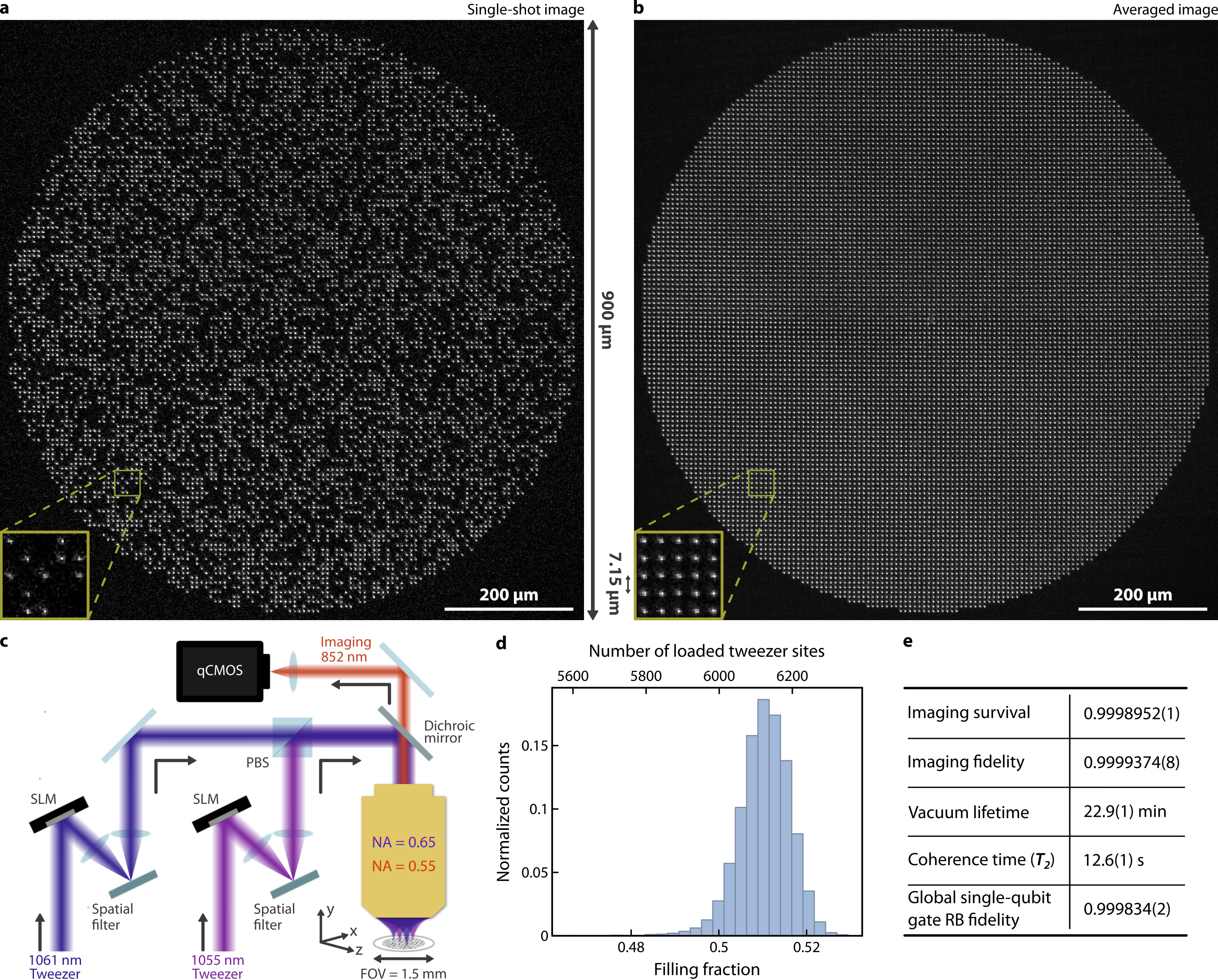
Figure 1: Large-scale tweezer array. a, Representative single-shot image of single cesium atoms across a 12,001 tweezer array. Inset: magnified view of a subsection of the stochastically loaded array. b, Averaged image of single atoms across a 12,001 tweezer array. Inset: magnified view of a subsection of the averaged array. Atoms are spaced by ${\sim}7.15\,\mu$m and held in 1061 nm and 1055 nm optical tweezers. c, Schematic of the optical tweezer array generation. Tweezer arrays, generated by two spatial light modulators (SLM), at 1061 nm and 1055 nm are combined with orthogonal polarization, and focused through an objective with a numerical aperture (NA) of 0.65 and a field of view (FOV) of 1.5 mm in diameter. The $y$-axis in the figure corresponds to the direction of gravity. We collect scattered photons from single atoms through the same objective (NA$=0.55$ at the imaging wavelength) and image them on a qCMOS camera. d, Histogram of filling fraction. We load 6,139 single atoms on average per experimental iteration. This corresponds to loading 51.2% of the array on average, with a relative standard deviation of 1.13% over 16,000 iterations. e, Summary of the key metrics demonstrated in this work. The imaging survival quoted is a steady-state imaging survival probability, and the global single-qubit gate fidelity is obtained from global randomized benchmarking (RB), as detailed in the text.

Here, we demonstrate a tweezer array with around 12,000 sites, that traps over 6,100 atomic qubits, simultaneously surpassing state-of-the-art values for metrics associated with fundamental limitations of the platform, including hyperfine qubit coherence time and trapping lifetime in a room-temperature apparatus, as well as combined imaging fidelity and survival (Fig. 1). Our results have implications for aforementioned applications in quantum science, in particular, concerning large-scale quantum computing and error correction, as discussed in more detail below.

Summary of approach and results
Our approach leverages high-power trapping of single atoms at far-off-resonant wavelengths in a specially designed, room-temperature vacuum chamber (Methods, Ext. Data Fig. 1a), enabling low-loss, high-fidelity imaging in combination with long hyperfine coherence times at the scale of 6,100 qubits (Fig. 1e). Specifically, we demonstrate imaging of single cesium-133 atoms with a survival probability of $99.98952(1)\%$, in combination with an imaging fidelity of $99.99374(8)\%$, surpassing the state-of-the-art achieved in much smaller arrays^{covey_2000-times_2019}. This, alongside a 22.9(1) minute vacuum-limited lifetime in our room-temperature apparatus ^{schymik_single_2021} — over three times longer than previous records for tweezer arrays in room-temperature apparatuses ^{covey_2000-times_2019} — provides realistic timescales for array operations in large scale arrays with minimal loss, e.g., for atomic rearrangement ^{barredo_atom-by-atom_2016, endres_atom-by-atom_2016, kim_situ_2016}.

Importantly, we further demonstrate a coherence time of 12.6(1) s, a record for a hyperfine qubit tweezer array, surpassing previous values by almost an order of magnitude ^{bluvstein_quantum_2022, graham_multi-qubit_2022} and approaching results for a single hyperfine qubit in a customized blue-detuned trap ^{tian_coherence_2023}, alkali atoms in an optical lattice ^{dudin_light_2013}, and nuclear qubits in a tweezer array ^{barnes_assembly_2022}. We also show a single-qubit gate fidelity of $99.9834(2)\%$ measured with global randomized benchmarking, limited by technical noise. We observe high uniformity across the sites in the array for loading probability (Ext. Data Fig. 2c), trap depth (Ext. Data Fig. 2d), imaging survival (Ext. Data Fig. 4a), scattering rate (Ext. Data Fig. 3d), and qubit frequency (Ext. Data Fig. 5d). Our results, when paired with other recent techniques for scaling single-site addressing ^{zhang_scaled_2024}, along with demonstrations of two-qubit gate operations ^{evered_high-fidelity_2023, ma_high-fidelity_2023, finkelstein_universal_2024} and qubit rearrangement ^{beugnon_two-dimensional_2007, bluvstein_quantum_2022}, indicate that high-fidelity universal quantum computing with about ten thousand atomic qubits could be a near-term prospect, providing a path towards QEC with hundreds of logical qubits ^{xu_constant-overhead_2023}.

Large-scale optical tweezer generation
We scale the optical tweezer array platform to around 12,000 tweezers, while prioritizing achieving long qubit coherence times and high fidelities (Fig. 1e). As such, we trap using near-infrared wavelengths, far-detuned from dominant electric-dipole transitions to minimize hyperfine qubit decoherence from photon scattering and dephasing processes ^{ozeri_hyperfine_2005, ozeri_errors_2007}. Cesium atoms possess the highest polarizability among the stable alkali metal atoms at near-infrared wavelengths where commercial fiber amplifiers routinely provide continuous-wave laser powers that exceed 100 W. Thus, a large number of traps can be generated with sufficient depth. A representative single shot image of the array is shown in Fig. 1a, and an averaged image is shown in Fig. 1b.

The atoms are spaced by ${\sim}7.15\,\mathrm{\mu m}$ and held in traps at 1055 nm and 1061 nm, generated using spatial light modulators (SLMs), whose hologram phases are optimized with a weighted Gerchberg-Saxton algorithm ^{kim_gerchberg-saxton_2019, kim_large-scale_2019} to uniformize the tweezer trap depth across the array (Methods). The tweezer light is combined with polarization and focused through a high numerical aperture objective with an unusually large field of view of 1.5 mm diameter that provides a large area for qubit trapping and manipulation in ultra-high vacuum (Fig. 1c). We measure an average trap depth of $k_{B}\times 0.20(1)$ mK, with a standard deviation of $11.4\%$ across all sites (Ext. Data Fig. 2d), enabling consistent loading probability per site.

Loading and imaging single atoms
We demonstrate uniform loading and high imaging fidelity across the sites in the array. To load single atoms in the tweezers, we cool and then parity-project ^{schlosser_sub-poissonian_2001} from a ${\sim}1.6$ mm $1/e^{2}$ diameter magneto-optical trap. Before imaging the atoms, we use a multi-pronged approach to filter out atoms in spurious off-plane traps, residual from the SLM tweezer creation (Methods).

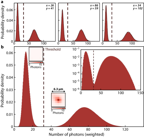
Figure 2: High-fidelity atom detection in a large-scale tweezer array. Imaging histogram showing the number of photons collected per site and per image. Note that the horizontal axes are weighted photon counts (see text); for non-weighted photon counts, see Ext. Data Fig. 3b. a, Imaging histogram of three randomly selected sites in the array (where $x$ and $y$ respectively denote the horizontal and vertical site indices in the array), and b, averaged over all sites in the array. Per-site histograms are fitted with a Poissonian model that integrates losses during imaging (Methods). The wide separation of peaks for empty and filled tweezers enables the high imaging fidelity presented in this work. The binarization threshold used to determine tweezer occupation is indicated by the vertical dashed line, and the average point-spread functions for the two classifications (atom absent and atom detected) are shown next to their corresponding peaks. Inset: the same histogram presented with a log-scale vertical axis. The weighted average relative error bar per bin is 0.08% (0.05% for the log-scale inset due to the smaller number of bins). Data for the histogram is collected from 16,000 iterations of the experiment.

We then zero the magnetic field and apply two-dimensional polarization gradient cooling (2D PGC) beams that are parallel to the atom array plane ($x$-$z$ plane in Fig. 1c) for fluorescence imaging of single atoms, which also simultaneously cool the atoms. The photons scattered from each atom are collected on a quantitative CMOS (qCMOS) camera for 80 ms, using the same objective with which the traps are created. We find that each site is loaded with a single atom on average 51.2% of the time with a relative standard deviation of 3.4% across the sites, demonstrating uniform filling of single atoms in a large tweezer array (Ext. Data Fig. 2c). This allows us to load over 6,100 sites on average in each iteration (Fig. 1d).

We detect and distinguish atomic presence in the array with high fidelity. Each image undergoes a binarization procedure (detailed in Methods) whereby each site is attributed a value of 0 (no atom detected) or 1 (one atom detected). Note that we detect no more than one atom ^{schlosser_sub-poissonian_2001} in each tweezer. We weight the collected photons in a $7\times 7$-pixel box centered around each site ^{cooper_alkaline-earth_2018}, so as to add more weight to pixels close to the center of each site’s point-spread function (Ext. Data Fig. 3a). The resulting signal is compared with a threshold to determine if an atom is present or not (Fig. 2).

We characterize the imaging fidelity, defined as the probability of correctly labeling atomic presence in a site, with a model-free approach, where no assumption is made about the photon distribution from Fig. 2. To this end, we identify anomalous series of binary outputs ^{norcia_microscopic_2018} in three consecutive images. For instance, $0\rightarrow 1\rightarrow 1$ would point to a false negative event in the first image, while $1\rightarrow 1\rightarrow 0$ could be due to atom loss during the second image or a false negative event in the third one. This approach allows us to precisely decouple inherent atom loss from false negatives or positives (Methods). From this we find an imaging fidelity of 99.99374(8)%. Crucial to this result are the homogeneous photon scattering rate across the array (Ext. Data Fig. 3d) and the consistency of the point-spread function even for sites at the edge of the array (waist radius of 1.7 pixels with a standard deviation of 0.2 pixels). Furthermore, we find that treating each site separately with an individual threshold only marginally improves the imaging fidelity to 99.9939(1)%, indicating that the imaging parameters are sufficiently consistent across the atom array. Finally, we estimate that the imaging fidelity in the absence of atomic loss would be closer to 99.999% (Methods).

Imaging survival and vacuum-limited lifetime
The probability of not losing a single atom in a tweezer array during imaging and due to finite vacuum lifetime both decrease exponentially in the number of atoms in an array, making these crucial metrics to optimize for large-scale array operation. The vacuum-limited lifetime, in particular, quantifies a fundamental experimental limitation on the amount of time in which operations can be executed without loss of an atom. This can, for example, be applied to give an upper limit on the fidelity with which one can achieve a defect-free array via atom rearrangement ^{barredo_atom-by-atom_2016, endres_atom-by-atom_2016}.

We probe the vacuum-limited lifetime by using an empirically optimized cooling sequence consisting of a 10 ms 2D PGC cooling block every 2 s. By fitting the exponential decay of the atom survival, we find a $1/e$ lifetime of 22.9(1) min (Fig. 3a). This is more than three times longer than the longest reported lifetime for neutral atoms in an optical tweezer array using a room-temperature apparatus ^{covey_2000-times_2019}, and only within a factor of 5 of the longest reported lifetime in a cryogenic apparatus ^{schymik_single_2021}. The result indicates that the probability of losing a single atom across the entire array remains under 50% during 100 ms, a relevant timescale for dynamical array reconfiguration and quantum processor operation.

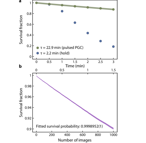
Figure 3: Long vacuum-limited lifetime and high imaging survival probability a, Vacuum-limited lifetime. Array-averaged survival fraction as a function of hold time is plotted. Two experiments are shown in the figure: with and without cooling. The green markers show data with a 10 ms 2D PGC block applied every 2 s (pulsed PGC), and the blue markers show the data without cooling (hold). The error bars are smaller than the markers. We find a $1/e$ lifetime of around 2.2 min without cooling. When the pulsed PGC block is applied, by fitting the data with $p(t)\propto\exp(-t/\tau)$, we find a vacuum lifetime of $\tau=22.9(1)$ min. b, Array-averaged survival fraction after many successive images. Between each image, we hold the atoms for 10 ms, without applying any cooling beams. We fit the data with $p(N)\propto p_{1}^{N}$, where $p(N)$ is the survival fraction after imaging $N$ times. From the fit, we find a steady-state imaging survival probability of $p_{1}=0.9998952(1)$. The light purple fill shows the estimated 67% confidence interval.

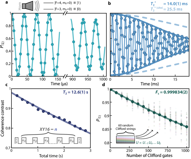
Figure 4: Long coherence times and high-fidelity single-qubit gates in a large atom array. a, Array-averaged Rabi oscillations between the hyperfine clock states $|0\rangle$ and $|1\rangle$. The fitted Rabi frequency is 24.611(1) kHz. The observed decay after several hundred microseconds stems from the spatially-varying Rabi frequency (Ext. Data Fig. 5c). b, Array-averaged Ramsey oscillations. During free evolution, the microwave drive field is detuned by 1 kHz, resulting in Ramsey oscillations. The characteristic decay time of these oscillations is $T_{2}^{*}=14.0(1)\,\mathrm{ms}$ fitting the average signal of all atoms. The light blue dashed line shows the decay time $T_{2}^{*(\mathrm{site})}=25.5\ \mathrm{ms}$ from fitting individual sites first and averaging the decay time afterwards. c, Measurement of the dephasing time $T_{2}$ after dynamical decoupling. After an initial $\pi/2$ pulse, a variable number of XY16 dynamical decoupling cycles with a fixed time $\tau=12.5\ \mathrm{ms}$ between $\pi$ pulses are used to offset the reversible dephasing. The phase of the final $\pi/2$ pulse is chosen to be either 0 or $\pi$, and subtracting the population difference in these two cases provides the coherence contrast. The contrast decay is fitted to obtain $T_{2}=12.6(1)\,\mathrm{s}$. d, Randomized benchmarking of the global single-qubit gate fidelity. For each number of Clifford gates, 60 different random gate strings of this length are applied, after which the overall inverse of the string is applied. The translucent markers represent the return probability for each string of gates, while the solid green markers indicate the averaged return probability over the 60 different strings. The decay of the final population to $1/2$ is fitted to $(1-d)^{N}$ and $F_{c}=1-d/2$ represents the average Clifford gate fidelity.

Moreover, we accurately characterize the imaging survival probability, without assuming any parameters, by performing 80 ms repeated imaging up to 1000 times, after which ${\sim}90$% of initially loaded atoms still survive (Fig. 3b). This corresponds to a steady-state imaging survival probability of $99.98952(1)\%$, mostly limited by vacuum lifetime. This, to the best of our knowledge, surpasses prior studies reporting record steady-state imaging survival using single alkaline-earth metal ^{covey_2000-times_2019} and alkali-metal ^{blodgett_imaging_parsed_2023} atoms in optical tweezers. These results, and the uniformity of imaging survival across the array (Ext. Data Fig. 4a), enable low-loss, high-fidelity detection of single atoms in large-scale arrays, crucial components for the practical use of the system (see Discussion and Outlook).

Qubit coherence
Key to recent progress in quantum computing and metrology with neutral atoms is the ability to encode a qubit in long-lived states of an atom, such as hyperfine states ^{bluvstein_quantum_2022, graham_multi-qubit_2022}, nuclear spin states ^{barnes_assembly_2022, huie_repetitive_2023, lis_midcircuit_2023, norcia_midcircuit_2023}, or optical clock states ^{norcia_seconds-scale_2019, madjarov_atomic-array_2019}. In cesium atoms, the hyperfine ground states ($|F=3,\ m_{F}=0\rangle\equiv|0\rangle$ and $|F=4,\ m_{F}=0\rangle\equiv|1\rangle$) provide such a subspace for storing quantum information. Furthermore, entanglement via Rydberg interactions can be readily transferred to this qubit to realize high-fidelity two-qubit gates ^{evered_high-fidelity_2023, finkelstein_universal_2024}. We now demonstrate the storage and manipulation of quantum information in a large-scale atom array by measuring the coherence time and global single-qubit gate fidelity. To this end we use a microwave horn to drive the hyperfine transition (Fig. 4a).

Preserving the coherence of a quantum system as it is scaled up is a known challenge across platforms for quantum computing and simulation ^{kjaergaard_superconducting_2020}. This difficulty persists even for neutral atoms, albeit at a lower level, due to residual interactions with a noisy and inhomogeneous electromagnetic environment, particularly with tweezers themselves (due to induced scattering and dephasing). Using far-off-resonant optical tweezers helps to preserve coherence, since the differential light shift of the hyperfine qubit decreases as $1/\Delta_{\mathrm{tweezer}}$ at constant trap depth, and the scattering rate as $1/\Delta_{\mathrm{tweezer}}^{3}$, where $\Delta_{\mathrm{tweezer}}$ is the tweezer laser detuning relative to the dominant electronic transition ^{kuhr_analysis_2005, ozeri_hyperfine_2005, ozeri_errors_2007}. We verify this by measuring a depolarization time of $T_{1}=119(1)$ s (Ext. Data Fig. 5e), and an ensemble dephasing time in the atom array of $T_{2}^{*}=14.0(1)$ ms (Fig. 4b), limited by trap depth inhomogeneity. Measured site-by-site, the dephasing time is $T_{2}^{*(\mathrm{site})}=25.5$ ms, consistent with being limited by an atomic temperature of ${\sim}4.8\ \mathrm{\mu K}$ during microwave operation ^{kuhr_analysis_2005}. We also measure the standard deviation of the qubit frequency in the array to be $1.5\times 10^{-9}$, or 14 Hz in absolute value (Ext. Data Fig. 5d).

The remaining reversible dephasing can be further mitigated by dynamical decoupling. By applying cycles of XY16 sequences ^{gullion_new_1990, souza_robust_2012} with a dwell time of 12.5 ms between $\pi$ pulses, the measured dephasing time is $T_{2}=12.6(1)$ s, thereby setting a new benchmark for the coherence time of an array of hyperfine qubits in optical tweezers ^{bluvstein_quantum_2022, graham_multi-qubit_2022} (Fig. 4c). Combined with recent advances in neutral atom quantum processors based on qubit transport ^{beugnon_two-dimensional_2007, bluvstein_quantum_2022, bluvstein_logical_2024}, which require dozens of microseconds for a set of parallel gates (and thus long coherence times), such long coherence times could enable the realization of complex quantum algorithms with thousands of qubits in the near-term.

Finally, we demonstrate global coherent single-qubit operation of our atom array and probe single-qubit gate fidelities through global randomized benchmarking ^{knill_randomized_2008, xia_randomized_2015, nikolov_randomized_2023}. To compensate for the inhomogeneous Rabi frequency across the array, which would result in pulse-length errors, we use the SCROFULOUS composite pulse ^{cummins_tackling_2003}. We apply gates sampled from the 24 unitaries composing the Clifford group $C_{1}$, followed by an inverse operation, and measure the final population in $|1\rangle$ (Fig. 4d). Fitting the decay as the number of gates increases yields an average Clifford gate fidelity $F_{c}=0.999834(2)$, limited by phase noise in our system likely due to magnetic field noise (Methods). This could be readily addressed by upgrading the current sources driving the magnetic field coils, shielding the vacuum cell, or by operating at MHz-scale by driving optical Raman transitions ^{levine_dispersive_2022}.

Discussion and outlook
We have demonstrated scaling of the optical tweezer array platform to over 6,100 individually-trapped atoms. While some crucial ingredients have yet to be demonstrated, especially the ability to rearrange atoms and entangle atomic qubits, we show equal or superior results to state-of-the-art experiments on several key metrics that are known bottlenecks for quantum computing, quantum simulation and quantum metrology. Notably, we achieve record-high imaging survival ^{covey_2000-times_2019} alongside competitive imaging fidelity. We measure record room-temperature vacuum-limited lifetime ^{covey_2000-times_2019} and coherence time in alkali metal atom tweezer arrays ^{bluvstein_quantum_2022, graham_multi-qubit_2022}, with a high global single-qubit gate fidelity, only limited by technical noise. We thereby largely circumvent aspects of degradation in classical and quantum control commonly faced by platforms as they are scaled up.

Our results usher in a new generation of neutral atom quantum processors based on several thousand of qubits, as well as large-scale programmable devices enabling advances in quantum metrology ^{rosenband_exponential_2013, ludlow_optical_2015, norcia_seconds-scale_2019, madjarov_atomic-array_2019, young_half-minute-scale_2020, finkelstein_universal_2024} and simulation ^{haferkamp_closing_2020, orourke_entanglement_2023, julia-farre_amorphous_2024}. For example, our platform — with the demonstrated qubit numbers — could be used for verifiable quantum advantage with low-depth evolution ^{haferkamp_closing_2020, ringbauer_verifiable_2023}. Tweezer clocks could be scaled using near-infrared, high-power tweezers for loading and imaging ^{tao_high-fidelity_2023} before transferring atoms to magic-wavelength traps for clock operation ^{norcia_seconds-scale_2019, madjarov_atomic-array_2019, young_half-minute-scale_2020, finkelstein_universal_2024}. We also foresee applications in quantum simulation for problems where boundary effects play an important role ^{bernien_probing_2017, browaeys_many-body_2020, ebadi_quantum_2021, scholl_quantum_2021, orourke_entanglement_2023}, which can be minimized with the large system sizes demonstrated here. In order to realize directions requiring interactions between atoms, we plan on exciting to Rydberg states ^{saffman_quantum_2010}. Promisingly, cesium provides a two-photon excitation pathway through the $7\textrm{P}_{3/2}$ intermediate state with a 455 nm lower photon transition and 1060 nm upper photon transition. With a large detuning from the intermediate state to minimize scattering, and with widely available laser powers at these wavelengths, it is possible to achieve Rabi frequencies as high as 5 MHz with minimal inhomogeneity across the full field of view.

Concerning universal quantum computation, the unusually large 1.5 mm field of view (FOV) of our objective provides enough space to engineer zones around our current array (900 $\mathrm{\mu m}$ in diameter) for interaction, storage, qubit rotation, and mid-circuit readout, enabling operations on qubits without disturbing adjacent atoms ^{beugnon_two-dimensional_2007, bluvstein_quantum_2022}. In order to utilize such a zone architecture for quantum computation, it is imperative to dynamically rearrange atoms across the optical tweezer array ^{barredo_atom-by-atom_2016, endres_atom-by-atom_2016}. Using commercially available acousto-optic deflectors with large field-of-view (${>}500\,\mathrm{\mu m}$ with our optical parameters) and fast steering mirrors, we foresee a straightforward pathway to low-loss transport of atoms across the complete objective field-of-view of 1.5 mm. This could be combined with recent technical developments that allow for high-speed parallel addressing of 10,000 sites ^{zhang_scaled_2024}, and demonstrations of ancilla-based mid-circuit readout techniques ^{singh_mid-circuit_2023, bluvstein_logical_2024, finkelstein_universal_2024}, to ultimately pave the way for repeated quantum error correction in neutral atom arrays with thousands of physical qubits.

For most quantum simulation and computation tasks, rearrangement of the stochastically loaded atom array into a defect-free array is required ^{barredo_atom-by-atom_2016, endres_atom-by-atom_2016}. The probability of obtaining a defect-free array can be limited by several factors, including finite imaging fidelity, imaging survival, imperfections in the rearrangement sequence, or finite vacuum-limited lifetime. We can provide an early estimate assuming a rearrangement time much less than our vacuum lifetime, that based on imaging survival alone, the probability to obtain a defect-free array of  6,040 rearranged atoms can be up to 39.5%, with optimal choices of imaging thresholding for this purpose (Ext. Data Fig. 4b). The average total number of defects corresponding to this estimation is 0.93.

Finally, our work indicates that further scaling of the optical tweezer array platform to tens of thousands of trapped atoms should be achievable with current technology, while essentially preserving high-fidelity control. In our present apparatus, several factors limit the number of sites. One limitation is the finite number of pixels of each SLM (which reduces the diffraction efficiency as the array size is increased), along with reduced SLM diffraction efficiency at higher incident laser powers. By using available higher-resolution SLMs, and by exploring techniques with higher pixel modulation depth ^{moreno_diffraction_2020}, we hope to utilize both power and field of view more efficiently. Furthermore, we observe worsening optical aberrations at tweezer powers greater than that in the present study due to thermal heating of the objective. This is the main limitation on atom number for the results in this work, even after aberrations were mitigated using the SLM (Methods). This constraint could be circumvented in the short term by dissipating heat from the objective more effectively to suppress detrimental aberrations and in the long term by utilizing an objective with a housing material that retains less heat; a combination of these upgrades should allow us to almost double the number of tweezers that we create using two fiber amplifiers. We further anticipate the potential to switch from polarization combination to wavelength-based array combination, opening up further avenues for increasing tweezer number with similar techniques. Atom numbers may further be increased in our array with the same number of tweezers by utilizing enhanced loading ^{brown_gray-molasses_2019} or re-loading techniques ^{shaw_dark-state_2023}. Already in the near-term, we expect to increase the number of atomic qubits to over ten thousand with the current system using a subset of these techniques.

Data availability

The data and codes that support the findings of this study are available from the corresponding author upon request.

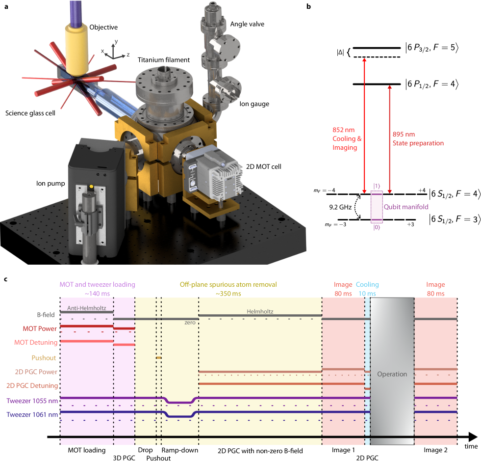
Figure 1: Experiment apparatus and sequence. a, Simplified view of the vacuum chamber. The 2D MOT cell (Infleqtion CASC) containing an electrically heated cesium dispenser, shown inside its integrated photonics assembly. This is attached to a stainless steel vacuum chamber on which an ion pump is mounted. We further use two titanium sublimation pumps (one mounted from the top, as shown, and one mounted from the bottom, not visible), sputtering almost the entire surface area of the chamber, except the rectangular part of the science glass cell and the ion pump. We use the following conventions for the laser beams: thick red for MOT beams, thin red for PGC beams, dark red (along $\hat{x}$) for state preparation beam, and purple for tweezer beam. b, Summary of the relevant states and transitions used in this work. c, Summary of a typical experimental sequence described in the Methods.

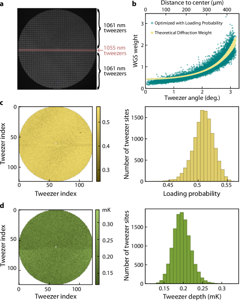
Figure 2: Tweezer uniformity details. a, The tweezers created by two fiber amplifiers, labeled so that they can be distinguished. We create 488 tweezers with 1055 nm light, and 11,513 tweezers with 1061 nm light. The 1055 nm tweezers fill the gap created by the spatial filtering of the 0^th order in the 1061 nm tweezer pathway, as described further in the tweezer generation section. b, The WGS weights given to tweezers during the tweezer homogenization procedure, as a function of angular distance from the 0^th order reflection off the SLM, with the physical distance this corresponds to given our optical setup shown on the upper axis. In teal is plotted the weights obtained after the tweezer depths are uniformized based on loading probability. In yellow is shown the weight compensation that would be expected based on diffraction efficiency calculations assuming blazed gratings are utilized for displacement. The weight increases with larger angle in order to compensate for the diminishing diffraction efficiency as a function of tweezer distance to the center. This additionally informs our decision to create a circularly shaped array. c, The per-site loading probability array map and its histogram. We feedback on the WGS trap depths based on the loading rate per site to uniformize the trap depth. We see an average loading probability per site of 51.2% with a relative standard deviation of 3.4%. The lowest loading probability is 25.1% for one tweezer, which is the only tweezer not shown in the histogram, but included in the quoted average. Note that three tweezers in the array are excluded for most of the data shown in this work, since they are affected by leakage from the 0^th order of the SLM on the 1061 nm tweezer pathway that is not completely extinguished via the spatial filtering. d, The per-site tweezer depth map and its histogram. This is obtained by measuring the differential light shift on $F=4\leftrightarrow F^{\prime}=4$ $D2$ transition ^{levine_quantum_2021}. We see an average trap depth of 0.20(1)mK with a standard deviation of 11.4% across the sites.

Figure 3: Imaging characterization. a, Weight function $W(u,v)$ applied to each pixel of the $7\times 7$ pixel box around each site. Here, $u$ and $v$ refer to the camera pixel coordinates centered on a given site. b, Imaging histogram obtained by summing the number of photons in the $7\times 7$ pixel box around each site, without any weights. c, Imaging fidelity as the binarization threshold is displaced from its optimal position. d, Map and histogram of the scattering rate per site across the tweezer array.

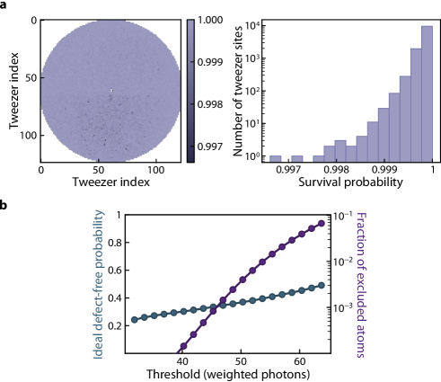
Figure 4: Imaging survival details. a, Map and histogram of the imaging survival probability per site across the tweezer array, as characterized using the three image analysis of data from 16,000 iterations. Note that the vertical axis of the histogram figure is plotted on a log scale. The mean of site-resolved imaging survival probability is 99.985%, and the minimum value 99.66%. b, Predicted upper bound on the probability of detecting a defect-free array after an ideal rearrangement sequence (estimated as $p(1|1)^{n}$ where $n$ is the number of atoms in the first image), limited by imaging survival and false positives. The threshold in the first image can be displaced to reduce false positives, at the cost of excluding some atoms. Note that we may ignore the issue of false negatives in the first image, since we can always physically eject residual atoms in sites that are determined to be negative.

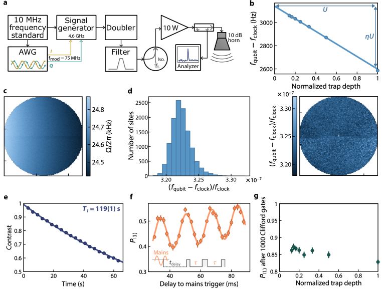
Figure 5: Characteristics of microwave-driven qubits. a, Schematic of the setup used to drive the hyperfine qubit. b, Estimation of $\eta$, the ratio of the differential polarizability of the hyperfine qubit to the electronic ground state scalar polarizability. The average qubit frequency is measured by Ramsey interferometry for different trap depths, and the slope is compared with the trap depth inferred from the light shift of the $F=4\leftrightarrow F^{\prime}=4$ $D2$ transition from its free-space resonance. c, Inhomogeneity of the Rabi frequency across the atom array. The reflection off a vertical metallic breadboard near the vacuum cell creates this spatial gradient orthogonal to the propagation axis of the microwaves. The Rabi frequency standard deviation is 0.5%. d, Relative difference of the qubit frequency with the cesium clock frequency $f_{\mathrm{clock}}=9,192,631,770$ Hz, measured by Ramsey interferometry. The standard deviation is $1.5\times 10^{-9}$, or 14 Hz in absolute value. e, Measurement of the depolarization time $T_{1}$. Atoms are initially prepared in $\left|1\right\rangle$. After a given time, the remaining population in $\left|1\right\rangle$ is measured, with or without a $\pi$ pulse before the measurement. The population difference, conditioned by the application of the pulse, constitutes the $T_{1}$ contrast. f, A spin-echo sequence is employed to probe the 60 Hz phase noise in our system. The free-evolution time of each arm, $\tau$, is set to a half-period of 60 Hz, which enhances the noise. By varying the time $t_{\mathrm{delay}}$ between the line trigger and the spin-echo sequence, we map the periodic noise at 60 Hz to the population in $\left|1\right\rangle$. g, The population in $\left|1\right\rangle$ after 1000 random Clifford gates is measured for different trap depths, exhibiting only limited improvement when the trap depth is reduced. In addition to other elements presented in the Methods, this indicates that the single-qubit gate fidelity is likely limited by residual magnetic field noise, which could be readily mitigated by technical improvements (Methods). Error bars indicate estimated 67% confidence intervals.

Methods

Vacuum apparatus

A schematic of our vacuum system is shown in Ext. Data Fig. 1. After the initial chamber assembly and multi-round baking process, we fire two titanium sublimation pumps (TSPs), mounted such that every surface except the rectangular portion of the glass cell and the interior of the ion pump are covered by line-of-sight sputtering. This creates a vacuum chamber in which essentially every surface is pumping. We do not find it necessary to re-fire the TSPs in order to maintain the vacuum level that we measure. We additionally maintain ultra-high vacuum conditions with an ion pump, connected to the primary chamber via a $45^{\circ}$ elbow joint. The secondary, science chamber consists of a rectangular glass cell (JapanCell) optically bonded to a 24 cm long glass flange (also sputtered by the TSP) that connects to the primary chamber. From lifetime measurements of tweezer trapped atoms (see main text) and collisional cross-sections available in literature ^{monroe_very_1990}, we estimate the pressure in the glass cell to be ${\sim}7\times 10^{-12}$ mbar, consistent with vacuum simulations using the MolFlow program ^{kersevan_recent_2019}.

Tweezer generation

We utilize light from two fiber amplifiers, at 1061 nm (Azurlight Systems) and 1055 nm (Precilasers) to create the optical tweezers through an objective (Special Optics) with NA$=0.65$ at the trapping wavelengths (NA $=0.55$ at the imaging wavelength of 852 nm) and a field of view of 1.5 mm. The tweezers are imprinted onto the light in each pathway by a Meadowlark phase-only Liquid Crystal on Silicon Spatial Light Modulator (SLM) that is water cooled to maintain a temperature of 22 ^∘C. On each path, there are two $4f$ telescopes utilized to map the SLM phase pattern onto the back focal plane of the objective, which subsequently focuses the tweezers into the vacuum cell as shown in Fig. 1c. In the first focal plane after the SLM, we perform spatial filtering on the two paths in order to remove the 0^th-order and reflect the 1^st-order diffracted light from the SLM. On the 1061 nm path we use two D-mirrors spaced by a few hundred microns, and on the 1055 nm path we use a mirror with a manufactured 300 $\mu$m hole as spatial filters to separate 0^th-order light from the tweezer light. The 1055 nm tweezers are essentially used to fill the gap between two halves of the array created by the 1061 nm tweezers (Ext. Data Fig. 2a), although we anticipate increasing the number of tweezers created with this path after implementing the objective heat-dissipation strategies as described in the discussion and outlook section.

While one would like to separate the 1^st order hologram phase pattern and 0^th order reflection in a more convenient manner, the largest angular separation that is possible between the 0^th and 1^st order of the SLM, as determined by the SLM pixel size, would not separate the large tweezer array from the 0^th order, due to the large angular distribution of the tweezers. Furthermore, the diffraction efficiency of the SLM into the 1^st order decreases with increasing separation from the 0^th order. Therefore, it is the most power-efficient choice to center the tweezers around the 0^th order, and to filter it at the first focal plane after the SLM. This decreasing diffraction efficiency with increasing distance from the 0^th order, at the center of the array, informs our choice of a circular tweezer array.

The SLM phase patterns are optimized with a weighted Gerchberg-Saxton (WGS) algorithm ^{kim_gerchberg-saxton_2019, kim_large-scale_2019} to create a tweezer array that we uniformize through a multi-step process, first adjusting weights in the algorithm based on photon count on a CCD camera that images the tweezers ^{nogrette_single-atom_2014}, and secondly adjusting weights based on the loading probability of each site in the atomic array with a variable gain feedback, as demonstrated on smaller arrays in previously developed schemes ^{schymik_situ_2022}. We implement around 5 iterations of each step in order to achieve the loading and survival probabilities that are shown in Ext. Data Figs. 2c, 4a. The WGS goal weight $W_{i}$ on each tweezer for the $i^{\textrm{th}}$ iteration is given by

$$W_{i}=\frac{1-G(1-\sqrt{H_{i}})}{\langle W_{i}\rangle},$$

normalized by the mean weight $\langle W_{i}\rangle$, where the height $H_{i}$ is determined by adjusting the value from the previous iteration using the loading probability per tweezer $P_{\textrm{load}}$, normalized by the average loading probability,

$$H_{i}=H_{i-1}\left[1-g\left(1-\frac{P_{\textrm{load}}}{\langle P_{\textrm{load}}\rangle}\right)\right].$$

We choose the weight of the gains $G$ and $g$ in order to reach convergence for the given configuration of tweezers (here we use a value of $0.6$ for each), and additionally add a cap to the allowable values of $H_{i}$ in order to avoid oscillatory behavior. We show in Ext. Data Fig. 2b, the weights for tweezers for different angular diffraction off of the SLM, obtained after utilizing the loading-based uniformization. We also show the theoretical weights that would be expected based on the inverse of the naive diffraction efficiency calculations for blazed gratings. The diffraction efficiency is given by $DE=\operatorname{sinc}{\frac{\pi ax}{2\lambda f}}\operatorname{sinc}{\frac{\pi ay}{2\lambda f}}$, where $a$ is the SLM pixel size, $x$ and $y$ are the horizontal and vertical displacements from the 0th order at the tweezer plane, $f$ is the effective focal length of the objective, and $\lambda$ is the trapping wavelength. We expect that some divergence in behavior could be due to angular-dependent transmission in optics in the imaging path.

We furthermore add aberration correction to the SLM phase hologram based on Zernike polynomials ^{levine_quantum_2021}. We perform a gradient-descent-type optimization to determine the amplitude of the Zernike polynomial coefficients by optimizing on the filling fraction in the array. We iterate between this optimization and 2-3 rounds of loading-based uniformization.

To align the tweezers created by the two fiber amplifiers in angle, we change the goal configuration for the WGS algorithm, and to align in the vertical and horizontal directions, we add a blazed grating to the SLM phase hologram. The CCD camera on which we image the tweezers after the vacuum cell provides a helpful reference for this alignment.

Loading single atoms in tweezers

The typical experimental sequence can be seen in Ext. Data Fig. 1c. From an atomic beam generated with a two-dimensional magneto-optical trap (2D MOT) of cesium-133 atoms (Infleqtion CASC), we load ${\sim}10^{7}$ atoms in the three-dimensional (3D) MOT in 100 ms using three pairs of counter-propagating beams in each axis and create a ${\sim}1.6$ mm $1/e^{2}$ diameter MOT cloud. The magnetic field gradient is set to 20 $\mathrm{G\,cm^{-1}}$ with a quadrupole configuration using a pair of coils that is perpendicular to the objective axis. Each beam has a size of 2.5 cm in diameter, detuning of $\Delta=-3.17\Gamma$ from the bare atom $|6S_{1/2},F=4\rangle\leftrightarrow|6P_{3/2},F^{\prime}=5\rangle$ resonant transition (Ext. Data Fig. 1b), and a total intensity of 10$I_{0}$ (1.6$I_{0}$ for repumping beams), where $I_{0}\approx 1.1\,\mathrm{mW\,cm^{-2}}$ is the saturation intensity of the transition between the stretched states, and $\Gamma\approx 2\pi\times 5.2\,\mathrm{MHz}$ is the natural linewidth of the $6P_{3/2}$ electronically excited state ^{steck_cesium_2023}. After loading atoms into the 3D MOT, we switch off the quadrupole magnetic field and, at the same time, lower the intensity to $7I_{0}$ and detune the laser further to $\Delta=-19.5\Gamma$ to cool atoms below the Doppler temperature limit via 3D polarization gradient cooling (PGC), which loads atoms into ${\sim}k_{B}\times 0.2$ mK depth tweezers, and parity projects the number of atoms in a tweezer ^{schlosser_sub-poissonian_2001} to either 0 or 1. This 3D PGC is applied for 40 ms, after which we wait another 40 ms for the remaining atomic vapor from the MOT to drop and dissipate. The optical tweezer array is kept on for the entirety of the experiment.

Generating optical tweezers with an SLM results in weak out-of-plane traps that can trap sufficiently cold atoms from the MOT ^{singh_dual-element_2022}. This could lead to a strong background in the image or to false positives detection of single atoms, both of which affect the imaging fidelity. To avoid this issue, we apply a resonant pushout beam for 2 $\mu$s, apply 2D PGC for 30 ms, quasi-adiabatically ramp-down the tweezer power to one-fifth of the full power, wait for 70 ms, then ramp-up the power. After this sequence, we apply 2D PGC for 180 ms with an added bias magnetic field of $0.19$ G. Note that this sequence for removing atoms in spurious traps was not fully optimized and we believe this can be readily shortened in future work.

Single-atom imaging

For single-atom imaging in the optical tweezers, we use four independent PGC beams, copropagating two-by-two along two orthogonal axes in the tweezer array plane. Each beam is overlapped with repumping beam and has a $1/e^{2}$ diameter of 3.5 mm, and 1.0 mW laser power in total (400 $\mu$W for repumping beam). Beams having axial components of the objective axis are not used as they would impart very high image background due to reflections off the uncoated glass cell surface. During imaging, we increase the total intensity of the 2D PGC beams for ${\sim}3\%$ and set the detuning to $\Delta=-15.5\Gamma$ from the bare atom $|6S_{1/2},F=4\rangle\leftrightarrow|6P_{3/2},F^{\prime}=5\rangle$ resonant transition. We collect scattered photons for 80 ms on a qCMOS camera (Hamamatsu ORCA-Quest C15550-20UP), which we choose for its fast readout time and its high resolution. The optical losses in the imaging system results in around 2.7% of scattered photons entering the camera, of which 44% are detected on the sensor due to the quantum efficiency at 852 nm. The total magnification factor of the imaging system is 5.1.

The averaged point-spread function waist radius is measured to be 1.7 pixels on the qCMOS camera, corresponding to $7.8\ \mathrm{\mu m}$ on the camera plane or $1.5\,\mathrm{\mu m}$ on the atom plane. We estimate that, accounting for a finite atomic temperature (up to $50\ \mathrm{\mu K}$ in this simulation) and camera sensor discretization, the ideal PSF radius should be 1.25 pixels. We leave an investigation of the discrepancy to future work.

Imaging model and characterization

We now describe the binarization procedure applied to each image acquired by the qCMOS camera. For each experimental run, typically consisting of a few hundred to a few thousand of iterations, we apply this procedure anew.

We identify all sites by comparing the average image with the known optical tweezer array pattern generated by the SLM. The signal for each site and each image is obtained by weighting the number of photons per pixel with a function $W(u,v)$ (Ext. Data Fig. 3a), which is optimized by numerical methods to maximize the imaging fidelity.

We then compare the signal obtained for each site and each image with a threshold to determine if an atom has been loaded. To position the threshold and estimate the fidelity, we employ two complementary methods: an analytical model that predicts the shape of the imaging histogram by integrating the loss probability in a Poisson distribution, and a model-free approach that estimates the fidelity by identifying anomalous atom detection results in three consecutive images. We use the first method to position the binarization threshold in most experimental runs, as well as for site-by-site analysis; we use the second method to accurately estimate the fidelity with a single array-wide threshold. The fidelities quoted in the main text are calculated using this second method.

We first describe the analytical model that predicts of the shape of histogram, which we call “lossy Poisson model”. We fit six parameters: the initial filling fraction (before the first image) $F$, the mean number of photons collected from the background light $\lambda_{0}$ and the atoms $\lambda_{1}$, the broadening from an ideal Poisson distribution $r_{0}$ and $r_{1}$, and the pseudo-loss probability $L$. The exact meaning of all parameters is described below.

We first derive this model in the absence of broadening from an ideal Poisson distribution. We are interested in the photon distribution given that there is no atom at a given site at the beginning of imaging $P(N=n|0)$ and the photon distribution given that there is an atom at this site at the beginning of imaging $P(N=n|1)$, where $N$ is the number of photons collected. For the background photon distribution, we simply assume a Poisson distribution: $P(N=n|0)=e^{-\lambda_{0}}\lambda_{0}^{n}/n!$. For the atom photon distribution we derive an expression by considering a loss-rate model where each photon collection event (occurring with probability $\lambda_{1}\mathrm{d}t$) imparts a loss probability $L/\lambda_{1}$. By integrating over $t\in[0,1]$ the system of equations that describes the evolution of the joint distribution of atom presence and photon count, we find the distribution given that one atom was initially present,

$$\begin{split}P&(N=n|1)=\frac{(\lambda_{0}+\lambda_{1}-L)^{n}e^{-(\lambda_{1}+\lambda_{0})}}{n!}\\ &+\frac{L}{\lambda_{1}}\frac{e^{\frac{\lambda_{0}L}{\lambda_{1}-L}}\left(1-\frac{L}{\lambda_{1}}\right)^{n-1}}{(n-1)!}\\ &\times\left[\Gamma\left(n,\frac{\lambda_{0}}{1-L/\lambda_{1}}\right)-\Gamma\left(n,\lambda_{1}+\frac{\lambda_{0}}{1-L/\lambda_{1}}\right)\right].\end{split}$$

Here, $\Gamma$ represents the upper incomplete gamma function. The real loss probability during imaging is then given by $\tilde{L}=1-e^{-L}$. The overall photon probability distribution is given by $P(N=n)=FP(N=n|1)+(1-F)P(N=n|0)$. For practical purposes we empirically include a broadening of the Poisson distribution by writing $P(N=n)=FP(N=n/r_{1}|1)/r_{1}+(1-F)P(N=n/r_{0}|0)/r_{0}$ and by effectively considering non-integer photon numbers (by replacing factorials with the gamma function). For large $n$ this amounts to considering a Gaussian distribution for either of the two peaks, but with the added benefit of including the loss through a physically-motivated derivation using a Poisson process.

In this model the true negative probability is given by $T$, $\mathcal{F}_{0}=\int_{0}^{T}{P(N=n|0)\mathrm{d}n}$; and the true positive probability, by $\mathcal{F}_{1}=\int_{T}^{\infty}{P(N=n|1)\mathrm{d}n}$. Finally the imaging fidelity can be estimated as $\mathcal{F}=F\mathcal{F}_{1}+(1-F)\mathcal{F}_{0}$ and the threshold $T$ can be found by maximizing the fidelity. We find that this model performs well when predicting the shape of the histogram site-by-site (Fig. 2a), but fails when the distribution of the background or atom photons in the array is non-Gaussian.

The second method we use to characterize imaging fidelity and survival requires no assumption for the photon distribution, but considers that the imaging survival and fidelity is identical for three successive images ^{norcia_microscopic_2018, madjarov_entangling_2021}. We start by estimating the probability $P_{x_{1}x_{2}x_{3}}$ of the presence of an atom in three images being $x_{1}x_{2}x_{3}$, where $x_{i}$ is a Boolean, equal to 1 if there is an atom and 0 if there is none,

$$\begin{split}\tilde{P}_{111}&=S^{2}F,\\ \tilde{P}_{110}&=(1-S)SF,\\ \tilde{P}_{100}&=(1-S)F,\\ \tilde{P}_{000}&=1-F.\end{split}$$

Here, $S$ is the survival probability during imaging and $F$ is the initial filling fraction. From this we can estimate the probability of detecting $y_{1}y_{2}y_{3}$ as $P_{y_{1}y_{2}y_{3}}=\sum_{x_{1}x_{2}x_{3}}P(y_{1}|x_{1})P(y_{2}|x_{2})P(y_{3}|x_{3})\tilde{P}_{x_{1}x_{2}x_{3}}$. The conditional probabilities on the detection categorization given the true atomic presence are $P(1|1)=\mathcal{F}_{1}$, $P(0|1)=1-\mathcal{F}_{1}$, $P(1|0)=1-\mathcal{F}_{0}$, and $P(0|0)=\mathcal{F}_{0}$.

We use the method of least squares to minimize the difference between the experimental frequencies of bitstrings $y_{1}y_{2}y_{3}$ and the $P_{y_{1}y_{2}y_{3}}$ by tuning the four parameters $F$, $S$, $\mathcal{F}_{0}$ and $\mathcal{F}_{1}$. The imaging fidelity is then defined as $\mathcal{F}=F\mathcal{F}_{1}+(1-F)\mathcal{F}_{0}$. The array-wide binarization threshold is chosen to maximize the imaging fidelity (Ext. Data Fig. 3c). Using this method, we find the survival to be $S=0.999864(2)$, slightly lower than the steady-state imaging survival probability measured by repeated imaging. Finally, we can inject the model-free survival probability into the lossy Poisson model to increase its accuracy (trying to extract the loss directly from the lossy Poisson model would indeed be very inaccurate, since losses appear as a small tail feature between the two peaks of the imaging histogram). Using this approach, and fitting each site independently, we find an average imaging fidelity of 99.992(1)%, in reasonable agreement with the model-free imaging fidelity. By setting the atom loss to zero while keeping the five other fit parameters constant for each site, we can estimate a hypothetical imaging fidelity in the absence of atomic loss of 99.999(1)%. This analysis also illustrates that fitting the imaging histogram with a Gaussian or Poissonian model without including losses leads to overestimating imaging fidelities ^{levine_quantum_2021}.

Note that in this section, we use images 2-4 of a set of 16,000 iterations containing each 4 successive images, since we a posteriori realize that the survival probability and imaging fidelity are significantly higher than for images 1-3. In this latter case we measure an imaging fidelity of 0.999882(1) and survival of 0.999817(2). This could be due to remaining background vapor from the MOT loading stage, or to imperfect background atom removal during the off-plane trapped atom push-out stage. In principle, we could obtain the same fidelity and survival from the first image by waiting more for the background vapor to diffuse in the chamber or by extending our push-out scheme.

Microwave setup

The setup used to drive microwave transitions is described in Ext. Data Fig. 5a. Similarly to other experiments ^{li_toward_2009, maller_single-_2015} the driving field is provided by RF modulation of a microwave oscillator. The timing reference is provided by the 10 MHz output signal from a Rubidium frequency standard (Stanford Research Systems FS725). An arbitrary waveform generator (AWG, Spectrum Instrumentation M4i.6622-x8) set at a sampling rate of 330 MSample/s IQ-modulates a microwave signal generator (Stanford Research Systems SG386) set at a fixed frequency of 4.6 GHz. The signal is then frequency-doubled, filtered, passed through an isolator before being amplified to 10 W of microwave power (Qubig QDA). A 10 dBi-gain pyramidal horn emits the microwave field on the atom array at a distance of 15 cm. By observing the return signal through a dual-directional coupler, we estimate that 7 W of power effectively reach the horn, resulting in a Rabi frequency of 24.6 kHz (Fig. 4a).

Qubit state preparation and readout

To initialize the tweezer-trapped atoms in the $|6S_{1/2},F=4,m_{F}=0\rangle\equiv|1\rangle$ state, we perform 5 ms of optical pumping on the $F=4\leftrightarrow F^{\prime}=4$ $D1$ transition. Simultaneously, we repump atoms in the $F=3$ hyperfine ground state on the $F=3\leftrightarrow F^{\prime}=4$ $D2$ transition. Both beams are coaligned and linearly polarized using a Glan-Thompson prism, parallel to the quantization axis defined by a 2.70 G bias magnetic field to drive $\pi$-transitions. The beams are focused with a cylindrical lens to a dimension of $3.3\,\mathrm{mm}\times 73\,\mu\mathrm{m}$ ($1/e^{2}$ waists) at the tweezer array. The peak intensity is ${\sim}0.043\,\mathrm{W}\mathrm{cm}^{-2}$ for the 895 nm $D1$ pump, and ${\sim}0.31\,\mathrm{W}\mathrm{cm}^{-2}$ for the 852 nm $D2$ repump. Angular momentum selection rules forbid the $m_{F}=0\leftrightarrow m_{F}^{\prime}=0$ transition for $\Delta F=0$, and the atomic population accumulates in $|1\rangle$ after multiple spontaneous emissions. We estimate a state preparation fidelity of 99.2(1)%, inferred from the early-time contrast of the Rabi oscillations in Fig. 4a. Factors that limit the state preparation include imperfect linear polarization purity, spatial variations in the pump laser intensity, and heating incurred during the optical pumping. Additionally, other state preparation schemes have been demonstrated previously on smaller arrays with higher preparation fidelity, and could be implemented in our system in the future ^{wu_sterngerlach_2019, evered_high-fidelity_2023}.

After preparing the atoms in $|1\rangle$, the trap depth is adiabatically lowered to $k_{B}\times 64\,\mathrm{\mu K}$ for microwave operation. For state readout we apply a resonant $|6S_{1/2},\ F=4\rangle\leftrightarrow|6P_{3/2},\ F^{\prime}=5\rangle$ pulse to push out atoms in $|1\rangle$, before imaging remaining atoms in $|0\rangle$ with the scheme described above.

Characterizing the atomic qubits

To characterize the Rabi frequency across the array, we drive the qubit for variable times and measure the population, averaged over initially loaded tweezer sites, in $|1\rangle$, both at early times (0-150 $\mu$s) and at late times (900-1000 $\mu$s). At late times we observe stripes in the final population in $|1\rangle$ due to spatially-varying Rabi frequency across the array (Ext. Data Fig. 5c). The observed gradient is orthogonal to the propagation axis of the microwave field, which points to a reflection off a vertical metallic optical breadboard next to the vacuum cell.

We also characterize the dephasing in the array using Ramsey interferometry. For this purpose, we observe the decay of Ramsey oscillations by applying a $\pi/2$ pulse, waiting for some time $\tau$ and applying another $\pi/2$ pulse. During the free-evolution, we detune the microwave drive field by $\delta=2\pi\times 1\ \mathrm{kHz}$ from the average qubit frequency. The envelope of the Rabi oscillation has a Gaussian decay with a characteristic time $T_{2}^{*}=14.0(1)$ ms. However, when considering each site individually we find an average $\langle T_{2}^{*(\mathrm{site})}\rangle=25.5$ ms with a standard deviation of 3.2 ms (in the per-site case we fit the oscillation decay with the dephasing decay function from Ref. ^{kuhr_analysis_2005}). This shows that dephasing across the array primarily occurs because of trap depth inhomogeneities (Ext. Data Fig. 2d): assuming a Gaussian distribution of trap depth with a standard deviation $\delta U$, the qubit frequencies in the array also follow a Gaussian distribution, which results in an ensemble-wide dephasing time $T_{2}^{*\mathrm{(inh)}}=\sqrt{2}\hbar/(\eta\,\delta U)$ where $\eta$ is the ratio of the ground state scalar differential polarizability to the electronic ground state polarizability ^{kuhr_analysis_2005} (Ext. Data Fig. 5b). On the other hand, finite atomic temperature limits the per-site dephasing time $T_{2}^{*(\mathrm{site})}$.

In order to relate $T_{2}^{*}$ and trap depth inhomogeneity or atomic temperature, we also calibrate the parameter $\eta$. Polarizability calculations exhibit significant disagreements ^{kuhr_analysis_2005, rosenbusch_ac_2009, carr_doubly_2016} so we find that an experimental approach yields more accurate results. For this purpose, we measure the average qubit frequency by performing a Ramsey measurement after an evolution time of $\tau=2$ ms, obtained by varying the second $\pi/2$ pulse’s phase between $-\pi$ and $\pi$. Thus, we measure the qubit frequency for different trap depths (Ext. Data Fig. 5b) and extract $\eta$ by comparing the change in frequency with the trap depth measured via depumping on the $|F=4\rangle\rightarrow|6P_{3/2},\ F^{\prime}=4\rangle$ transition. We find $\eta=1.22(6)\times 10^{-4}$, with an uncertainty primarily limited by the unknown distribution of $m_{F}$-states population during the depumping experiment. This allows us to estimate the atomic temperature during microwave operation as ^{kuhr_analysis_2005} $T=0.97\times 2\hbar/(\eta k_{B}\langle T_{2}^{*(\mathrm{site})}\rangle)\approx 4.8\ \mathrm{\mu K}$ (provided the temperature is sufficiently homogeneous to invert the fraction and the mean). We note that this temperature may differ from the effective atomic temperature in other iterations of the experimental sequence that do not include the rampdown and state preparation steps that may decrease and increase the temperature respectively. On the one hand, the trap depth is adiabatically ramped down compared with its maximum level by a factor of 3 (which decreases the temperature by a factor $\sqrt{3}$); on the other hand, the state preparation procedure induces some heating due to the repeated scattering events required to prepare the atoms in $|1\rangle$.

Dynamical decoupling

In order to extend the operation time of a realistic quantum processor well beyond the dephasing time of the array, we can apply dynamical decoupling on the atomic qubits ^{bluvstein_quantum_2022}. Selecting an appropriate dynamical decoupling sequence and dwell time between $\pi$ pulses is critical to cancel as much noise as possible ^{souza_robust_2012}. In this work, we empirically find the symmetric XY16 sequence to perform slightly better than symmetric XY8, and equivalent sequences with Knill composite pulses ^{souza_robust_2011}. A persistent 60 Hz phase noise in our system precludes dwell times close to multiples of a half-period of 60 Hz. We find that a dwell time of 12.5 ms yields the longest dephasing time.

We vary the number of XY16 cycles and we obtain the coherence contrast by applying a final $\pi/2$ pulse with phase 0 or $\pi$. Subtracting the population difference in these two cases yields the coherence contrast after the dynamical decoupling sequences.

Randomized benchmarking

In addition to dynamical decoupling, we measure our single-qubit gate fidelity via randomized benchmarking, similarly to Refs. ^{xia_randomized_2015, nikolov_randomized_2023}. For each given length $n$, we select $U_{n-1},\dots,U_{0}$ at random from the 24 unitaries composing the Clifford group. We then apply $U_{-1}U_{n-1}\cdots U_{0}$ where $U_{-1}$ is the inverse of $U_{n-1}\cdots U_{0}$. We decompose Clifford gates into elementary rotations around Bloch sphere axes using the $zyz$ Euler angles. Rotations around $z$ are implemented by offsetting the phase of all following $x$ and $y$ rotations. This comes from the fact that ^{mckay_efficient_2017} $e^{-i\frac{\theta}{2}\sigma_{x}}e^{-i\frac{\theta_{z}}{2}\sigma_{z}}=e^{-i\frac{\theta_{z}}{2}\sigma_{z}}e^{-i\frac{\theta}{2}(\cos(\theta_{z})\sigma_{x}+\sin(\theta_{z})\sigma_{y})}$ and similarly when exchanging $x$ and $y$.

Due to the inhomogeneous Rabi frequency, each rotation must be applied using length error-resilient (PLE) composite pulses. Several families of PLE-resilient pulses have been described, and after comparison of three of them (BB1 ^{wimperis_broadband_1994, cummins_tackling_2003}, SCROFULOUS ^{cummins_tackling_2003} and SCORBUTUS ^{kukita_short_2022}), we find that SCROFULOUS performs the best in our case. The SCROFULOUS implements a rotation of angle $\theta$ around the axis indexed by the angle $\phi$ on the Bloch sphere equatorial plane (abbreviated as $\theta_{\phi}$) with a symmetric composite pulse $(\theta_{1})_{\phi_{1}}(\theta_{2})_{\phi_{2}}(\theta_{3})_{\phi_{3}}$ where $\theta_{1}=\theta_{3}=\mathrm{arcsinc}(2\cos(\theta/2)/\pi)$, $\phi_{1}=\phi_{3}=\phi+\arccos{\left(-\frac{\pi\cos{\theta_{1}}}{2\theta_{1}\sin(\theta/2)}\right)}$, $\theta_{2}=\pi$ and $\phi_{2}=\phi_{1}-\arccos{\left(-\frac{\pi}{2\theta_{1}}\right)}$. In our implementation, the average pulse area for a random Clifford unitary is $2.02\pi$.

We fit the decay of the final population with the number of applied Clifford gates as $\frac{1}{2}+\frac{1}{2}(1-d_{0})(1-d)^{n}$ where $d_{0}$ stems from SPAM errors, $d$ is the average depolarization probability at each gate and $n$ is the number of gates. The average Clifford gate fidelity is then given by ^{knill_randomized_2008}: $F_{c}=1-d/2$.

Even though the measured single-qubit gate fidelity is competitive with other state-of-the-art atom arrays experiments ^{wang_single-qubit_2016, graham_multi-qubit_2022, ma_universal_2022, bluvstein_logical_2024}, single-qubit gate fidelities ${>}0.9999$ have been reported ^{sheng_high-fidelity_2018, nikolov_randomized_2023} in smaller arrays. Moreover, the maximal theoretical fidelity achievable for a given dephasing time is ^{xia_randomized_2015} $\mathcal{F}=\frac{3}{4}+\frac{1}{4(1+0.95(t/T_{2}^{*})^{2})^{3/2}}$ where $t$ is the average time needed to apply a Clifford gate, $t=\langle\theta\rangle/\Omega$; $\langle\theta\rangle$ being the average pulse area per Clifford gate. Hence, gate fidelities higher than 0.99999 should be achievable solely based on this value.

Beyond infidelities due to decoherence, other parameters that may limit single-qubit gate fidelities are: (a) amplitude errors due to instabilities in the microwave power; (b) phase errors due to the microwave setup; (c) phase errors due to optical tweezer intensity noise; (d) phase errors due to magnetic field noise. We are interested in which of these factors is limiting the gate fidelity. We rule out (a) because we observe that the Rabi frequency is very stable shot-to-shot (variations of less than 0.1 %), and we estimate that such variations should be completely suppressed by the SCROFULOUS pulse. We also rule out (c) since reducing the trap depth further does not significantly improve the randomized benchmarking results (Ext. Data Fig. 5g). Although we cannot formally rule out (b), we estimate that it is unlikely since active components in the microwave setup have a very low phase noise, and we observe a sub-10 Hz linewidth of the microwave signal with a spectrum analyzer.

We also notice a dominant phase noise at 60 Hz in the qubit array due to the mains AC voltage. We measure the intensity of this noise with a spin-echo sequence, where the time between each pulse is $\tau=1/(2\times 60\ \mathrm{Hz})$ (Ext. Data Fig. 5f). Although this low-frequency noise cannot by itself explain the single-qubit gate fidelity loss, it points out more generally to residual magnetic field noise that could be mitigated by shielding the vacuum cell, upgrading the current sources driving the magnetic field coils, and/or by operating at MHz-scale via Raman transitions by shining two laser beams detuned by 9.2 GHz ^{yavuz_fast_2006, jones_fast_2007}, or by amplitude-modulating a single beam with diffractive optics ^{levine_dispersive_2022}.

Quantifying uncertainties in atom survival-based experiments

Much of the data presented in this work is based the measurement of atom survival after applying a specific experimental sequence. For a fixed set of experimental parameters, the survival is averaged over all iterations (individual experiments) and all sites where an atom is initially loaded. Because of our large number of atoms, the binomial uncertainty $\sqrt{p(1-p)/\sum_{i=1}^{N}{n_{i}}}$ (where $p$ is the mean atom survival probability, $N$ is the number of iterations, and $n_{i}$ is the number of initially loaded atoms in each iteration), used by many atom array experiments, is unreasonably small and does not reflect the real uncertainty, dominated by shot-to-shot environmental fluctuations.

Hence, we use the following model instead: we consider $N$ iterations where, for each iteration $i$, $n_{i}$ atoms are initially loaded. The atom survival for each atom $j$ at iteration $i$ is represented by a Bernoulli random variable $B_{ij}$, where $B_{ij}=1$ corresponds to when the atom survived and $B_{ij}=0$ corresponds to when the atom did not survive. For each iteration $i$ we assume that the $\{B_{ij}\}_{j}$ are independent and identically distributed with a random probability $P_{i}$. The $\{P_{i}\}_{i}$ are also independent and identically distributed and follow a distribution with mean $p$ and variance $\sigma^{2}$. We are interested in the mean survival by iteration $S_{i}=(\sum_{j}{B_{ij}})/n_{i}$ and the global survival $S=(\sum_{i}{S_{i}})/N$. Using the law of total variance, we find that

$$\mathrm{Var}(S)=\frac{1}{N^{2}}\sum_{i}{\left(\sigma^{2}\left(1-\frac{1}{n_{i}}\right)+\frac{1}{n_{i}}p(1-p)\right)}.$$

Assuming $n_{i}\approx n$, which stands in this work, we finally obtain: $\mathrm{Var}(S)=\frac{1}{N}(\sigma^{2}(1-1/n)+p(1-p)/n)$. In practice, we estimate the uncertainty on the mean survival for a given set of experimental parameters by

$$\varepsilon=\sqrt{\frac{1}{N}\left(\frac{N}{N-1}V_{S}+\frac{p(1-p)}{n}\right)},$$

where $V_{S}$ is the sample variance of the mean survival per iteration ($\simeq\mathrm{Var}(S_{i})$ in the model), $n$ is the mean number of atoms loaded per iteration, $p$ is the mean survival over all iterations, and $N$ is the number of iterations.