On dark matter effect on BH accretion disks

Abstract

Comparing different dark matter (DM) models, we explore the DM influence on the black hole (BH) accretion disk physics, considering co-rotating and counter-rotating thick accretion tori orbiting a central spinning BH. Our results point out accretion onto a central BH as a good indicator of the DM presence, signaling possible DM tracers in the accretion physics. We analyze accretion around a spinning BH immersed in perfect-fluid dark matter, cold dark matter and scalar field dark matter. Our investigation discusses observational evidence of distinctive DM effects on the toroidal accretion disks and proto-jets configurations, proving that BHs accretion tori, immersed in DM, can present characteristics, such as inter–disks cusp or double tori, which have been usually considered as tracers for super-spinars and naked singularity attractors. Therefore in this context DM influence on the BH geometry could manifest as super-spinars mimickers. DM affects also the central spinning attractor energetics associated with the accretion physics, and its influence on the accretion disks can be searched in a variation of the central BH energetics as an increase of the mass accretion rates.

I Introduction

In this work we study the dark matter (DM) influence on the black hole (BH) accretion disk physics, investigating the accretion disks morphology for co-rotating and counter-rotating geometrically thick accretion tori orbiting a central spinning BH. Comparing three different DM models, our analysis points out possible observational evidence of distinctive DM effects on the accretion disks, which can be traces for the DM presence. Our investigation does not cover all the admissible parametric DM values for the deformed metrics but, taking into account constraints formerly obtained by the study of orbits, the DM BH shadows, or the emission spectra, we perform a comparative analysis of the DM models and an investigation on the constraints imposed on the accretion discs, aimed at further restricting the parameters range and pointing out the possible DM mark in some accretion features. From a methodological viewpoint we take advantage of axial symmetry of DM metrics, studying fully general relativistic models of stationary toroidal orbiting configurations.

The physics of accretion disks around BHs and super massive black hole (SMBH), hosted in quasars and active galactic nuclei (AGN), powers the most energetic processes of our Universe, often accompanied with ejection of matter in jet-like structures with extremely large radiative energy output. We investigate the DM effects on these aspects, focusing on SMBH at the center of galaxies and the accretion discs empowering the emissions. We analyze particularly the limiting situation of static (and spherically symmetric) background (with spin parameter $a=0$) and the DM deformation on the Kerr extreme BH spacetime (with spin value $a=M$), seeing significant qualitative detectable variations with respect to the standard vacuum BH case. Many astrophysical observations lead to SMBH hosted at the galactic center embedded in a DM halo, and in metric models considered here the central BH is surrounded by DM envelope that modifies the geometry around the BH, not interacting directly with the accreting matter or its radiation.

More generally there is a large amount of observational evidence of the presence of some kind of DM component in our Universe, for example from the galactic rotation curves and galaxy cluster dynamics. However, within the variety of the different observations pointing at the DM presence, there is no single metric that encompasses all the DM effects in a single model, and which could also explain the absence of DM observed at different scales. In this work we consider a spinning BH immersed in perfect fluid DM (PFDM) [4, 5, 6, 7], cold dark matter (CDM) and scalar field dark matter (SFDM)–[8, 9].

These DM models have been extensively studied in recent literature. PFDM model was considered in [5] and the effects of PFDM on particle motion around a static BH in an external magnetic field were studied in [10]. The shadow of the spinning BH in PFDM was studied in [4], whereas in [6] geodesic motion in PFDM Kerr and Kerr-anti-de Sitter/de Sitter BH were studied–see also [7]. For studies of the geodesic in the Kerr-de Sitter spacetimes see [11, 12, 13, 14, 15]. In [16] superradiance and stability of Kerr DM enclosed by anisotropic fluid matter were studied. Spinning BH solutions with quintessential energy have been discussed in [17]. In [8] BH in DM halo was considered. Rotating black holes with an anisotropic matter field was considered in [18], while in [9] there is a discussion of the BH shadow of Sgr A* in DM halo. Superradiance and instabilities in BHs surrounded by anisotropic fluids were considered in [19]. Galactic dark matter in the phantom field model was considered in [20]. The case of rotating (Kerr) naked singularities was treated in [21, 22, 23, 24]. Here we focus on the influence of DM on BHs governing toroidal accretion structures.

There is an extensive literature exploring the DM effects on the BH and BH accretion physics. Since DM influences different aspects of the singularity, from the characteristics of the horizon (for example it can manifest itself in the BH shadows) to the energetics properties of the surrounding matter, there are various assessments of the DM effects and parameter constraints on the models describing DM presence around BHs. In [26] for example DM clouds of axions around BHs were studied with superradiant instabilities and accretion which could manifest on the gravitational wave signal induced by a small compact object in the field of the central BH–see also [27, 28]. More recently in [29] the formation of SMBHs at high redshifts was studied in connection with ultralight DM, see also [30, 31] for growth of accretion driven scalar DM hair around a Kerr BHs. The DM effect on the quasinormal modes of massless scalar field and electromagnetic field perturbations in a BH spacetime surrounded by PFDM was considered in [32]. An analysis of DM in the M87 core in relation to BH shadows effects was presented in [33], see also [35] and shadows of Sgr A* BH surrounded by superfluid DM halo was studied in [34], and shadow from a charged rotating BH in presence of PFDM is explored in [36].

The DM candidates are various, including string and brane theory effects, boson clouds, hypothetical new particles, primordial BHs and alternative theories of gravity. From the observational view-point, dark matter can be detectable from the products of its decay or annihilation in cosmic rays, gamma rays, neutrinos or even gravitons–see also [37], and gravitational–wave and neutrino astronomy can then open different windows in the DM analysis. DM comprehension, particularly focused on sub-galactic DM halos, is also a goal of the Webb Telescope .

Nevertheless, despite the variety of DM models, the standard cosmological model is in fact the $\Lambda$-CDM, which includes a cosmological constant ($\Lambda$) (with negative pressure), encoding Dark energy (DE) in empty space (or vacuum energy) explaining the Universe accelerating expansion. (In this scenario the effects of the cosmological constant are also treated as quintessence.) Polytropic models of DM halos in $\Lambda$-CDM cosmology were individuated in [45]. In this model, the DM velocity is less than the speed of light (in this respect neutrinos component are excluded, being non-baryonic but not necessarily cold) and it is dissipationless as it is not cooled by radiating photons. CDM may be constituted by an hypothetical weakly interacting massive particle (WIMPS), or primordial BHs, or axions.

Although considered a DM standard model, CDM is not exempt from various problems, emerging for example from the observations of galaxies and galaxy clusters and clusterization emerging from the rotation curves and morphological studies (as the cuspy halo problem). There is also a more general problem in describing the effects and presence of DM at large and small scales. The CDM model collides therefore with small-scale structure observations. For all these reasons the search for alternative DM models is still an open issue, and in this respect the SFDM model seems to adapt to both large-scale and small-scale structure observations while the PFDM seems capable to explain the asymptotically flat rotation velocity characterizing the spiral galaxies.

In this analysis we study geometrically thick accretion disk models, Polish Doughnuts (P-D), orbiting the central attractor, whose center coincides with the equatorial plane of the central axisymmetric attractor[62, 47, 48, 49, 50]. These thick accretion tori are characterized by very high (super-Eddington) accretion rates and high optical depth. Tori morphology and stability are essentially governed by the pressure gradients on the equatorial plane [47]. The thin (Keplerian) disks can be considered as P-D limiting configurations regulated by the background geodesic structure. The DM background metric has a characteristic geodetic structure constituting a first major constraint on accretion physics. The tori, described by purely hydrodynamic (barotropic) models, are governed by the equipressure surfaces that can be closed, giving stable equilibrium configurations, and open, giving unstable, jet-like (proto-jets) structures caused by the relativistic instability due to the Paczynski mechanism where the effects of strong gravitational fields are dominant with respect to the dissipative ones and predominant to determine the unstable phases of the systems [57, 51, 58, 59, 60, 53, 54, 61].

Many features of the tori dynamics and morphology like their thickness, their stretching in the equatorial plane, and the location of the tori are predominantly determined by the geometric properties of spacetime via a fluid effective potential function. Consequently, in models where DM is geometrized as a metric deformation, DM has a clear impact in the tori structure, modifying the fluid effective potential. The gradients of the effective potential on the tori equatorial and symmetry plane regulate the pressure gradient of the fluid in the Euler law governing dynamics of the perfect fluid [62]. The special case of cusped equipotential surfaces is related to the accretion phase onto the central attractor [62, 47, 48, 60, 63]. The outflow of matter through the cusp occurs due to an instability in the balance of the gravitational and inertial forces and the pressure gradients in the fluid, i.e., by the so called Paczynski mechanism of violation of mechanical equilibrium of the tori [48].

DM affects the cusp formation and cusp location with respect to the central singularity, modifying the disk accretion throat, constraining the thickness of the accretionary flow and the maximum amount of matter swallowed by the central BH. Consequently DM will influence the energetic characteristics of the BH in accretion and the disk characteristics, as accretion rates or cusp luminosity [64, 65, 66].

More in details plan of the article is as follows: Thick disks in axially symmetric spacetimes are discussed in Sec. (II). The Kerr metric is introduced in Sec. (II.1). The Polish doughnut tori models are detailed in Sec. (II.2). The fluid effective potential is the subject of Sec. (II.2.1). Extended geodesic structure, constrained the tori modes is explored in Sec. (II.2.2). Dark matter models are discussed in Sec. (III). In Sec. (III.1) the perfect fluid dark matter is considered. Cold and scalar field dark matter models are studied Sec. (III.2). Discussion and conclusions follow in Sec. (IV).

II Thick disks in axially symmetric spacetimes

We study geometrically thick tori in axially symmetric DM–BH spacetimes, considered as a DM-induced deformation of the Kerr geometry. Therefore it is useful here to review the properties of the Kerr metric and the construction of tori in this geometry. More specifically, in Sec. (II.1) the Kerr metric is introduced, while the Polish doughnut tori models are discussed in Sec. (II.2).

II.1 The Kerr metric

The Kerr metric is an axially symmetric, asymptotically flat, vacuum exact solution of the Einstein equation describing the spacetime of central spinning compact object. According to the metric parameter values (dimensionless spin $a/M$), the Kerr metric describes naked singularities (NSs) for $a>M$ and black holes (BHs) for $a\in[0,M]$. The Kerr BH geometry has the limiting static solution of Schwarzschild for $a=0$ and the extreme Kerr BH spacetime for $a=M$.

In the Boyer-Lindquist (BL) coordinates $\{t,r,\theta,\phi\}$, the metric tensor reads:

$$ds^{2}=-\left(1-\frac{2Mr}{\Sigma}\right)dt^{2}+\frac{\Sigma}{\Delta}dr^{2}+\Sigma d\theta^{2}+\left[(r^{2}+a^{2})+\frac{2Mra^{2}}{\Sigma}\sin^{2}\theta\right]\sin^{2}\theta d\phi^{2}-\frac{4rMa}{\Sigma}\sin^{2}\theta dtd\phi,$$ (1)

where

$$\Delta\equiv a^{2}+r^{2}-2rM;\quad\Sigma\equiv a^{2}(1-\sigma)+r^{2},\quad\sigma\equiv\sin^{2}\theta,$$ (2)

with $G=c=1$. The horizons $r_{-}<r_{+}$ are respectively given by

$$r_{\pm}\equiv M\pm\sqrt{M^{2}-a^{2}},$$ (3)

the horizons can be found by solving the equation $a=a_{\pm}\equiv\sqrt{r(2M-r)}$ for $r\in[0,2M]$ . The outer and inner stationary limits $r_{\epsilon}^{\pm}$ (ergosurfaces) (solutions of $g_{tt}=0$) are respectively

$$r_{\epsilon}^{\pm}\equiv M\pm\sqrt{M^{2}-a^{2}(1-\sigma)},$$ (4)

the ergosurfaces can be found by solving the equation $a=a_{\epsilon}^{\pm}\equiv{a_{\pm}}/{\sqrt{1-\sigma}}$ (for $\sigma\neq 1$), where $r_{+}<r_{\epsilon}^{+}$ on $\theta\neq 0$ and $r_{\epsilon}^{+}=2M$ in the equatorial plane $\theta=\pi/2$ ($\sigma=1$). Static observers, with four-velocity $\dot{\theta}=\dot{r}=\dot{\phi}=0$(where $\dot{q}$ indicates the derivative of any quantity $q$ with respect the proper time (for time-like particles) or a properly defined affine parameter for the light-like orbits) cannot exist inside the (outer) ergoregion, but trajectories $\dot{r}\geq 0$, including particles crossing the stationary limit and escaping outside in the region $r\geq r_{\epsilon}^{+}$ are possible.

The constants of the geodesic motions are

$$\mathcal{E}=-(g_{t\phi}\dot{\phi}+g_{tt}\dot{t}),\quad\mathcal{L}=g_{\phi\phi}\dot{\phi}+g_{t\phi}\dot{t},\quad g_{ab}u^{a}u^{b}=-\mu^{2},$$ (5)

with $u^{a}\equiv\{\dot{t},\dot{r},\dot{\theta},\dot{\phi}\}$. In Eqs (5) quantities $\mathcal{E}$ and $\mathcal{L}$ represent the total energy and momentum of the test particle coming from radial infinity, as measured by a static observer at infinity.

The relativistic angular velocity and the specific angular momentum are

$$\Omega\equiv\frac{u^{\phi}}{u^{t}}=-\frac{\mathcal{E}g_{\phi t}+g_{tt}\mathcal{L}}{\mathcal{E}g_{\phi\phi}+g_{\phi t}\mathcal{L}}=-\frac{g_{t\phi}+g_{tt}\ell}{g_{\phi\phi}+g_{t\phi}\ell},\quad\ell\equiv\frac{\mathcal{L}}{\mathcal{E}}=-\frac{u_{\phi}}{u_{t}}=-\frac{g_{\phi\phi}u^{\phi}+g_{\phi t}u^{t}}{g_{tt}u^{t}+g_{\phi t}u^{\phi}}=-\frac{g_{t\phi}+g_{\phi\phi}\Omega}{g_{tt}+g_{t\phi}\Omega},$$ (6)

respectively. The sign of $\mathcal{L}(\ell)$ defines the co-rotation/counter-rotation of the particles (fluid). The DM models are axis-symmetric and stationary and we define similarly notion of co-rotating and counter-rotating motions.

II.2 Geometrically thick tori: the Polish doughnut models

We specialize our analysis to the Polish doughnut (P-D) tori, general relativistic hydrodynamic (GRHD) toroidal configurations centered on the central BH equatorial plane, which is coincident with the tori equatorial symmetry plane.

These toroidal models are well known and used in different contexts. They are analytic and general relativistic models defined and integrable in axis symmetric spacetimes, where the results known as the "von Zeipel theorem" hold, ensuring the integration condition on the equations for the fluid. For this reason we here apply these results to the stationary DM metric models.

Tori are composed by a one particle-species perfect fluid, where

$$T_{ab}=(\varrho+p)u_{a}u_{b}+pg_{ab},$$ (7)

is the fluid energy momentum tensor, $\varrho$ and $p$ are the total energy density and pressure, respectively, as measured by an observer moving with the fluid. The timelike flow vector field $u^{a}$ denotes the fluid four-velocity. The fluid dynamics is described by the continuity equation and the Euler equation respectively:

$$u^{a}\nabla_{a}\varrho+(p+\varrho)\nabla^{a}u_{a}=0,\quad(p+\varrho)u^{a}\nabla_{a}u^{c}+\ h^{bc}\nabla_{b}p=0,$$ (8)

where the projection tensor $h_{ab}=g_{ab}+u_{a}u_{b}$ and $\nabla_{a}g_{bc}=0$.

We assume a barotropic equation of state (EoS) $p=p(\varrho)$ and the stationary and axially symmetric matter distribution moves on circular trajectories. We investigate the case of a fluid toroidal configuration defined by the constraint $u^{r}=0$, as for the circular test particle motion no motion it is assumed in the $\theta$ angular direction, which means $u^{\theta}=0$. Because of these symmetries, the continuity equation is identically satisfied and the orbiting configurations are regulated by the Euler equation for the pressure $p$ only, which can be written as

$$\frac{\partial_{a}p}{\varrho+p}=-{\partial_{a}}W+\frac{\Omega\partial_{a}\ell}{1-\Omega\ell},\quad\mbox{with}\quad W\equiv\ln V_{eff},\quad\mbox{and}\quad V_{eff}=u_{t},$$ (9)

where $V_{eff}$ is the torus effective potential. Tori are regulated by the balance of the hydrostatic and centrifugal factors due to the fluid rotation and by the curvature effects of the background, encoded in the effective potential function $V_{eff}$.

Assuming the fluid is characterized by the specific angular momentum $\ell$ constant (see also discussion [55]), we consider the equation for $W:\;\ln(V_{eff})=\rm{c}=\rm{constant}$ or $V_{eff}=K=$constant. By setting $\ell=$constant as a torus parameter, the maximum density points in the disk, the pressure gradients (from the Euler equation) are determined by the gradients of the tori effective potential function. The maximum points of the tori effective potential as function of the radial coordinate provide the minimum points of pressure, where fluid particles are free on unstable circular geodetic orbits.

II.2.1 The fluid effective potential

The fluid effective potential (9) is explicitly [58, 71]

$$V_{eff}^{2}=\left(\frac{\mathcal{E}}{\mu}\right)^{2}={\frac{g_{t\phi}^{2}-g_{\phi\phi}g_{tt}}{g_{\phi\phi}+2g_{t\phi}\ell+g_{tt}\ell^{2}}}.$$ (10)

The extremes of the pressure are regulated by the angular momentum distributions $\ell^{\pm}:\partial_{r}V_{eff}=0$, on the equatorial plane $\theta=\pi/2$ for co-rotating $(-)$ and counter-rotating $(+)$ fluids respectively.

Torus cusp $r_{\times}$ is the minimum point of pressure and density in the torus corresponding to the maximum point of the fluid effective potential. The torus center $r_{center}$ is the maximum point of pressure and density in the torus, corresponding to the minimum point of the fluid effective potential. At the cusp ($r\leq r_{\times}$) the fluid may be considered pressure-free. Fluid effective potential defines the function $K(r)=V_{eff}(\ell(r))$. Cusped tori have parameter in the open ranges$K=K_{\times}\equiv K(r_{\times})\in]K_{center},1[\subset]K_{mso},1[$, where $K_{center}\equiv K(r_{center})$. (We adopt the notation $q_{\bullet}\equiv q(r_{\bullet})$ for any quantity $q$ evaluated on a radius $r_{\bullet}$.)

II.2.2 Extended geodesic structure and notable radii

The geometry equatorial circular geodesic structure constrains the accretion disk physics governing, in the P-D model, the tori cusps and centers locations. In the Kerr geometry the geodesic structure is constituted by the marginally circular orbit for timelike particles $r_{mso}^{\pm}$, which is also a photon circular orbit, $r_{mco}^{\pm}\equiv r_{\gamma}^{\pm}$, the marginally bounded orbit, $r_{mbo}^{\pm}$, and the marginally stable circular orbit, $r_{mso}^{\pm}$ (see Figs (1)). Radii $\{r_{mso}^{\pm},r_{mbo}^{\pm},r_{mco}^{\pm}\}$ constrain the location of the tori cusps (inner edges) with fluid specific angular momentum $\ell=\ell^{\pm}$ respectively

$$\mbox{where}\quad r_{mco}^{\pm}<r_{\mathrm{mbo}}^{\pm}<r_{\mathrm{mso}}^{\pm}<r_{\mathrm{(mbo)}}^{\pm}<r_{(mco)}^{\pm},$$ (11)

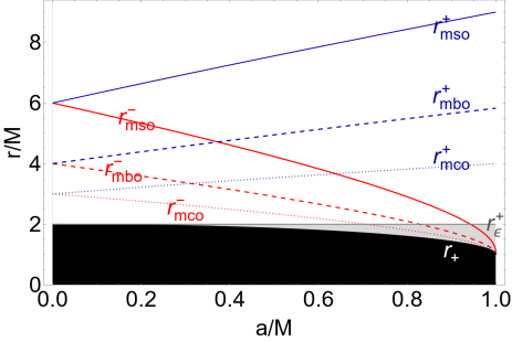
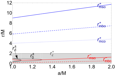
Figure 1: Geodesic equatorial circular structure of the Kerr geometry for spin $a\in[0,M]$ (left panel) and $a>M$ (right panel), for co-rotating ($(-)$-red-curves) and counter-rotating ($(+)$- blue curves) orbits. The marginally stable orbits ($mso$) are the solid curves, the marginally bounded orbits ($mbo$) are dashed curves, and marginally circular orbits $r_{mco}^{\pm}$ (which are also photon circular orbits) are the dotted curves. (Note for $a>M$ there is no last co-rotating circular orbit (i.e. $r_{mco}^{-}=0$.) Radius $r_{+}$ is the outer horizon, $r_{\epsilon}^{+}$ is the outer ergosurface on the equatorial plane. Black region is $r<r_{+}$ and gray region is $r\in[r_{+},r_{\epsilon}^{+}]$ for Kerr BHs and $r\in[0,r_{\epsilon}^{+}]$ for Kerr NSs. On radii $r_{0}^{\pm}$ (black dashed curve-right panel) there is $\mathcal{L}=0$ (where $\mathcal{L}$ is the test particle angular momentum) and on $r_{\delta}^{\pm}$ (black curve-right panel) there is $\mathcal{E}=0$ (where $\mathcal{E}$ is the test particle energy).

where we introduced also the radii $(r_{\mathrm{(mbo)}}^{\pm},r_{(mco)}^{\pm})$ defined as

$$r_{\mathrm{(mbo)}}^{\pm}:\;\ell^{\pm}(r_{\mathrm{mbo}}^{\pm})=\ell^{\pm}(r_{\mathrm{(mbo)}}^{\pm})\equiv\mathbf{\ell_{\mathrm{mbo}}^{\pm}},\quad r_{(mco)}^{\pm}:\ell^{\pm}(r_{mco}^{\pm})=\ell^{\pm}(r_{(mco)}^{\pm})\equiv\mathbf{\ell_{mco}^{\pm}},$$

significant as governing the location of the tori centers, More precisely ranges $(\mathbf{L_{1},L_{2},L_{3}})$ of fluids specific angular momentum $\ell$ govern the tori topology, according to the geodesic structure of Eqs (11), as follows:

$\mathbf{L_{1}}$:

for $\ell\in\mathbf{L_{1}}$ there are quiescent (i.e. not cusped) and cusped tori–where there is $\mp\mathbf{L_{1}}^{\pm}\equiv[\mp\ell_{mso}^{\pm},\mp\ell_{mbo}^{\pm}[$. The cusp is $r^{\pm}_{\times}\in]r^{\pm}_{mbo},r^{\pm}_{mso}]$ (with $K_{\times}^{\pm}<1$)) and the center with maximum pressure in $r^{\pm}_{center}\in]r^{\pm}_{mso},r^{\pm}_{(mbo)}]$.

$\mathbf{L_{2}}$:

for $\ell\in\mathbf{L_{2}}$ there are quiescent tori and proto-jets (open-configurations) –where there is $\mp\mathbf{L_{2}}^{\pm}\equiv[\mp\ell_{mbo}^{\pm},\mp\ell_{mco}^{\pm}[$. The cusp $r_{\times}^{\pm}\in]r_{mco}^{\pm},r_{mbo}^{\pm}]$ is associated to the proto-jets, with $K_{\times}>1$, and the center with maximum pressure is in $r_{center}^{\pm}\in]r_{(mbo)}^{\pm},r_{(mco)}^{\pm}]$. Proto-jets are associated to (not-collimated) open structures, with matter funnels along the BH rotational axis–see [59, 74, 75, 76];

$\mathbf{L_{3}}$:

for $\ell\in\mathbf{L_{3}}$ there are only quiescent tori where there is $\mp\mathbf{L_{3}}^{\pm}\equiv\mp\ell\geq\mp\ell_{mco}^{\pm}$ and the torus center is at $r^{\pm}_{center}>r_{(mco)}^{\pm}$.

In the metric models we consider, the DM affects the orbiting fluids modifying the Kerr axially symmetric geometry and the fluid effective potential–see also [78]. Therefore we study the radii limiting the tori construction, defined through the fluid effective potential for the geometries modified by the DM. More precisely we identify the marginally circular orbit, $r_{mco}^{\pm}$, as the radius $r_{mco}^{\pm}:K^{\pm}(r)=\infty$, the marginally bounded orbit defined by $r_{mbo}^{\pm}:K^{\pm}(r)=1$ (asymptotically flat spacetimes) and the marginally stable orbits $r_{mso}^{\pm}:\partial_{r}\ell^{\pm}=0$.

The orbiting fluid is governed by the geodesic structure of the considered spacetime. The tori are specified by the profile of the distribution of the specific angular momentum of the orbiting matter, (in the equator) and its relation to the radial profile of the specific angular momentum of equatorial circular geodesics. The so called Keplerian distribution of the circular geodesic angular momentum related to a given spacetime is generally given by the relation

$$\ell=\ell_{K}\equiv\frac{\Phi_{o}\mp\sqrt{\Phi\Phi_{(-)}^{2}}}{\Phi_{\star}},\quad\mbox{where}\quad\Phi_{(\mp)}\equiv g_{t\phi}^{2}\mp g_{tt}g_{\phi\phi},\quad{\Phi}\equiv\left(g_{t\phi}^{\prime}\right)^{2}-g_{tt}^{\prime}g_{\phi\phi}^{\prime},$$ (12)

$$\Phi_{o}\equiv g_{t\phi}^{\prime}\Phi_{(+)}-g_{t\phi}\left(g_{\phi\phi}g_{tt}\right)^{\prime},\quad\Phi_{\star}\equiv g_{t\phi}^{2}g_{tt}^{\prime}+g_{tt}^{2}g_{\phi\phi}^{\prime}-g_{tt}(g_{t\phi}^{2})^{\prime},$$

for $\theta=\pi/2$, where $(^{\prime})$ is for the derivative with respect to $r$. The Keplerian profile intersection with the tori profile determines centers and cusps of the tori. In the standard Kerr spacetime it takes the well known form:

$$\ell_{K}(r,a)=\ell^{\mp}\equiv\frac{a^{3}\mp r^{3/2}\Delta-a(4M-3r)r}{a^{2}-(r-2M)^{2}r}.$$ (13)

III Dark matter models

We analyze accretion tori orbiting spinning BHs with spacetimes influenced by different DM models. The metrics reduce, for some limiting values of the DM parameters reduces to the Kerr BH geometry. Thus, using Eqs. (10) we consider the BH DM metric components $\{g_{tt},g_{t\phi},g_{\phi\phi}\}$ in BL coordinates, and we refer to the literature for details on the metric tensor and the geometry properties. We investigate the equatorial circular geodesic structures for the fluid effective potential, the effective potential function and the tori structure for co-rotating and counter-rotating tori, in three DM models: in Sec. (III.1) we address the perfect fluid DM (PFDM) model of [4]. Cold and scalar field DM models of [9, 8] are discussed Sec. (III.2).

III.1 Perfect fluid dark matter (PFDM)

A rotating BH solution in perfect fluid dark matter (PFDM) has been discussed in [4], with

$$g_{tt}=-\left[1-\frac{2Mr-f_{D}(r)}{\Sigma}\right],\quad g_{t\phi}=-\frac{\sigma a[2Mr-f_{D}(r)]}{\Sigma},\quad g_{\phi\phi}=\sigma\left[\frac{a^{2}\sigma[2Mr-f_{D}(r)]}{\Sigma}+\left(a^{2}+r^{2}\right)\right],$$ (14)

$$g_{rr}\equiv\frac{\Sigma}{\Delta_{{D}}},\quad g_{\theta\theta}=\Sigma$$ (15)

$$\mbox{where}\quad\Delta_{D}\equiv\Delta+f_{D}(r)\quad\mbox{and}\quad f_{D}(r)\equiv kr\log\frac{r}{|k|},$$

see also [5, 6, 7], where $k$ is the parameter describing the intensity of the PFDM, set in the ranges $k\in]-7.18M,2M[$. For $k=0$ the line element reduces to the Kerr metric. The metric singularities, $r_{\pm}$, defining the DM deformations on the Kerr horizons, can be found by solving the equation $a=a_{\pm}\equiv\sqrt{r(2M-r)-f_{D}(r)},$ or from the equation $k=k_{\pm}\equiv\Delta/[rW\left({\Delta}/{r^{2}}\right)]$, where $W$ is the Lambert function, such that $W(z)$ gives the principal solution for $w$ in $z=we^{w}$.

The deformed ergosurfaces $r_{\epsilon}^{\pm}$ can be found, for $\sigma\neq 1$, as solution of the equation $a=a_{\epsilon}^{\pm}\equiv{a_{\pm}}/{\sqrt{1-\sigma}}$ while, on the equatorial plane $(\sigma=1)$ there is

$$r_{\epsilon}^{\pm}=\begin{cases}kW\left[\frac{e^{2M/k}}{\text{sgn}(k)}\right]<2,\quad\mbox{for}\quad k\lessgtr 0,\\ kW\left[-1,-e^{2M/k}\right]>2,\quad\mbox{for}\quad k<0,\\ 2,\quad\mbox{for}\quad k=0\end{cases}$$ (16)

(see red curve in Figs (2)–bottom left panel) where the Lambert function $W(s,z)$ gives the $s^{\text{th}}$ solution for $w$ in $z=we^{w}$, and $\text{sgn}(k)$ gives the sign of $k$, therefore it is $-1,0,1$ for $k$ negative, zero, or positive.

The PFDM horizons are independent of $\sigma$ (like in the Kerr case). The PFDM ergosurfaces are independent of spin in the equatorial plane (like in the Kerr cases). The horizons $r_{\pm}$ (and the ergosurfaces $r_{\epsilon}^{\pm}$ on the equatorial plane of Eq. (16)) are shown in Figs (2).

The red curve in Figs (2), which represents the BH horizon for $a=0$ (and the ergosurfaces Eq. (16) on the equatorial plane for $a\neq 0$), bounds the collections of horizons at different $a=$constant in the plane $(r/M,a/M)$. The PFDM metric describes solutions with $0$,$1$, and $2$ horizons. For BH solutions, horizons can be shifted outwardly or inwardly with respect to the Kerr BH spacetime depending on the value of $k$. There are also spacetime solutions with horizons for $a>M$.

Accordingly we select the PFDM metric parameter in the following six cases

$$\mathbf{k_{6}}\equiv\{k_{a}=-2M,k_{b}\approx-1.399M,k_{c}=-0.1M,k_{d}=0.1M,k_{e}\approx 0.82M,k_{f}\equiv 2M\}.$$ (17)

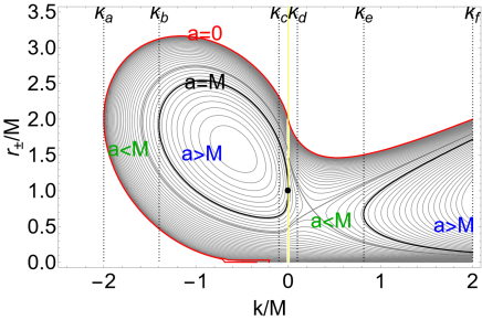
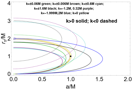
Figure 2: Horizons and ergosurfaces of the BHs in perfect fluid dark matter (PFDM) of Eq. (14). Different values of the $k\in]-7.18M,2M[$ parameter, describing the PFDM intensity, are considered. (For $k=0$ the line element describes the Schwarzschild and Kerr geometries in absence of DM.) Upper left panel: horizons $r_{\pm}$ as functions of the $k$ parameter, for different values of the spin $a\geq 0$. Curves at $a\lesseqgtr M$ are shown. Red curves are the horizons of the static case ($a=0$) (and the ergosurfaces $r_{\epsilon}^{\pm}$ Eqs (16) on the equatorial plane for $a>0$). Values $\mathbf{k_{6}}$ of Eq. (17) are signed as dotted vertical lines. Yellow vertical line labels the Schwarzschild and Kerr geometries in absence of DM. Upper right panel: the horizons $r_{\pm}/M$ as functions of the spin $a/M$ for different values of $k>0$ (solid curves) and $k<0$ (dashed curves). There is $k=\pm 0.06M$ (green), $k=\pm 0.006M$ (brown), $k=\pm 0.6M$ (cyan), $k=\pm 1.6M$ (black), $k=-1.2M,0.32M$ (purple), $k=-1.999M,2M$ (blue). Curve $k=0$ (yellow) represents the Schwarzschild and Kerr geometries in absence of DM. Bottom right and left panels: different views of horizons $r_{\pm}$ as functions of $k/M$ and $a/M$, mesh-functions are curves with constant $r/M$ (solid green), $k/M$ (dotted gray), and $a/M$ (solid red). Yellow vertical plane labels the case $k=0$. Function contour colors are according to the $a/M$ values (left panel) and $k/M$ values (right panel). We have marked with a black spot the extreme Kerr BH horizon $(a=M,r=M)$ on all panels. To highlight better this point plane $a=M$ (blue) is included in the bottom panels (the crossing of $a=M$ and $k=0$ planes occurs at the point $a=M,k=0,r=M$).

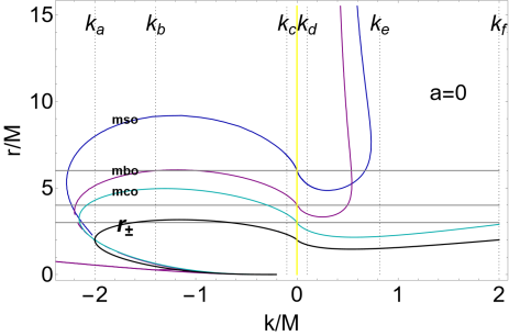
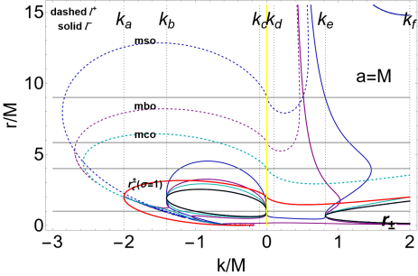
Figure 3: Equatorial circular geodesic structures of the Kerr attractor in perfect fluid dark matter (PFDM) of Eq. (14). Different values of the $k\in]-7.18M,2M[$, describing the PFDM intensity are considered, where for $k=0$ (vertical yellow line) the line element describes the Schwarzchild (for $a=0$) and extreme Kerr BH geometry (for $a=M$). Values $\mathbf{k_{6}}$ of Eq. (17) are signed with dotted vertical lines. Right panel shows the situation for $a=M$, left panel is for $a=0$. Radii $r_{\pm}$ are the horizons, $r_{\epsilon}^{\pm}$ are the ergosurfaces on the equatorial plane (coincident with the horizons of the static case). $mso$ is for marginally stable orbit, $mbo$ is for the marginally bounded orbit, $mco$ is for marginally circular orbit, for co-rotating fluids ($\ell=\ell^{-}$, solid curves) and counter-rotating fluids ($\ell=\ell^{+}$, dashed curves). Horizontal gray lines show the radii of the geodesic structure for the Kerr and Schwarzschild BH geometry in absence of dark matter ($k=0$) for $a=0$ and $a=M$ respectively. See also Figs (1).

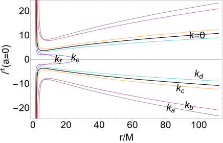
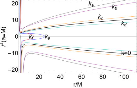
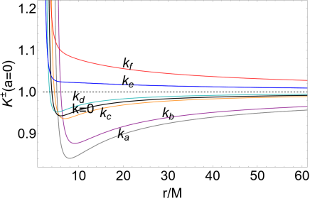
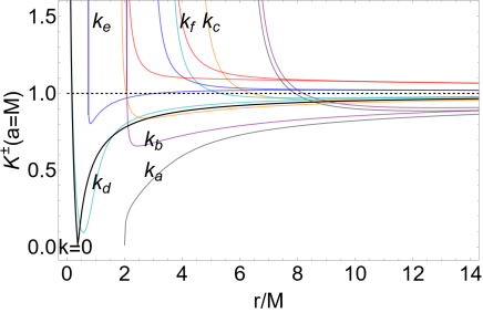
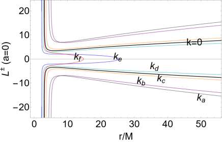
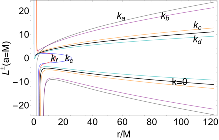
Figure 4: Fluid specific angular momentum $\ell^{\pm}$, energy parameter $K^{\pm}$ and (test particles) Keplerian angular momentum $\mathcal{L}^{\pm}$ as function of $r/M$ for co-rotating and counter-rotating fluids, different perfect fluid dark matter (PFDM) parameters of Eq. (14) signed on the panels. Different values of the $k\in]-7.18M,2M[$ parameter, describing the PFDM intensity, are considered. Columns are $a=0$ (left) and $a=M$ (right), and rows are $\ell^{\pm}$ (top), $K^{\pm}$ (middle), $\mathcal{L}^{\pm}$ (bottom). (For $k=0$ the line element describes the Schwarzschild or the Kerr geometry.) Values $\mathbf{k_{6}}$ are in Eq. (17).

The cases $(k_{a},k_{f})$ have as horizon $r=2M$ for $a=0$ (the static case) therefore, in this sense, these solutions can be compared to the Schwarzschild case. Similarly, for $k=k_{b}$, the geometry with $a=M$ has one horizon at $r=2M$. There is one horizon when $k=k_{e}$ and $a=M$.

In Figs (4) we show also the fluid specific angular momentum distribution for the $\mathbf{k_{6}}$ parameters, for the cases $a=0$ and $a=M$, compared to the distribution on the geometry in absence of DM (see also Figs (1)), the associated $K$ parameter and the Keplerian (test particle) angular momentum $\mathcal{L}^{\pm}\equiv\ell^{\pm}K^{\pm}$ respectively, which we have defined as related to the thick tori counterparts from definition of $K(r)\equiv V_{eff}(\ell(r))$, showing influence of the DM on the limiting thin Keplerian (geodesic) disk. The thin Keplerian disk is constrained by the geodesic structure of the gravitational background.

In general the geodesic structure is qualitatively similar for any spin–Figs (3). We focus on the two limiting cases $a=0$ and $a=M$, whose equatorial circular geodesic structures for the orbiting configurations are represented in Figs (3). In this model DM couples with the BH rotation, entangling with the frame dragging, evidenced in the deformed rotational law $\ell^{\pm}$ of the orbiting matter. According to the DM parameter $k$ and spin $a$, relation (11) i.e. $r_{mso}^{\pm}>r_{mbo}^{\pm}>r_{mco}^{\pm}$ for $\ell=\ell^{\pm}$ cases holds, similarly to the non deformed BH case. According to the discussion of Sec. (II.2.2) for the Kerr background, this relation, for small magnitude of $k$, reflects in the relative location of the maximum-minimum points of pressure of the orbiting disks. For values of $k$ where this relation is not verified, for example for $k>0$ of Figs (3), the orbiting toroidal structures show large qualitative divergences with respect to the accretion tori formation and dynamics in the Kerr BH spacetime.

–The static attractor ($a=0$) The geodesic structure is represented in Figs (3)-left panel, compared with the Schwarzschild case. We note that for $k>0$ the situation changes qualitatively with respect to the case in absence of DM. In Figs (4) is the fluid specific angular momentum $\ell^{\pm}$, the tori energy parameter $K^{\pm}$ and (test particles) Keplerian angular momentum $\mathcal{L}^{\pm}$ as function of $r/M$, for different PFDM parameters of Eq. (14), compared with the case $k=0$ describing the Schwarzschild geometry. Notably, for $(k_{f},k_{e})$, there is $K(r)>1$. From the $(\ell^{\pm},K^{\pm})$ analysis it is noted how, for some values of $k$, curves are lower with respect to the corresponding curves in absence of DM–Figs (3). From the analysis of the curves $L^{\pm}$, we can note how in some case the test particle angular momentum is qualitatively different from the corresponding in the Schwarzschild case. Tori and effective potentials in this case are represented in Figs (5), constrained by the geodesic structure of Figs (3).

–The spinning attractor ($a>0$) The geodesic structure for the spinning attractor geometry in PFDM is in Figs (3)–right panel. The fluid specific angular momentum $\ell^{\pm}$, energy parameter $K^{\pm}$ and (test particles) Keplerian angular momentum $\mathcal{L}^{\pm}$ are shown in Figs (4) as functions of $r/M$ for co-rotating and counter-rotating fluids and PFDM parameters of Eq. (14), compared to the case $k=0$ describing the Kerr geometry in absence of DM. Tori effective potentials for the counter-rotating (co-rotating) fluids are in Figs (6). Tori are in Figs (7) and Figs (8).

As clear from Figs (3) the geodesic structure in the DM geometry with $a=0$ is similar to the counter-rotating geodesic structure in the axially symmetric spacetime $(a\neq 0)$. The co-rotating case (for $a=M$), $\ell=\ell^{-}$, especially for $k>0$, is remarkably different from the geodesic structure in the geometries with $a=0$ and it is further complicated by the presence of the ergoregion deformed by the PFDM with, however, quantitative discrepancies with respect to the Kerr spacetime for large part of the DM parameter values $k<0$. For larger $k>0$ there are also NS solutions (also for $a\in]0,M]$) and, for even large values of $k>0$, there are BH solutions (also for $a>M$).

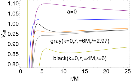
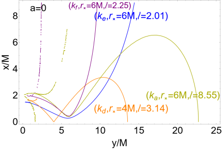
Figure 5: Case $a=0$. Tori orbiting BHs in perfect fluid dark matter (PFDM) of Eq. (14). Right panel shows the tori for selected values of the $k/M$ parameter, cusp location $r_{\times}$ and fluid specific angular momentum $\ell$, signed on the curves. Left panel shows the associated tori effective potentials. Values $\mathbf{k_{6}}$ of Eq. (17) are considered. (For $k=0$ the line element describes the Schwarzschild geometry.) There is $r=\sqrt{x^{2}+y^{2}}$ and $\sigma=y^{2}/(x^{2}+y^{2})$, where $\sigma\equiv\sin^{2}\theta$.

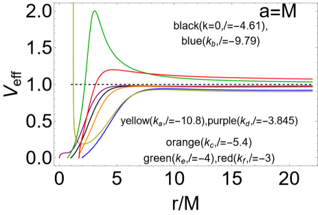
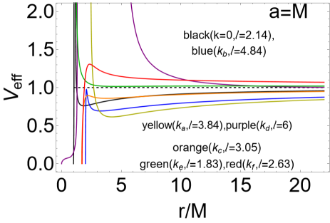
Figure 6: Case $a=M$. Effective potentials for the tori orbiting BHs in perfect fluid dark matter (PFDM) of Eq. (14), for different values of the parameter $k\in]-7.18M,2M[$, describing the PFDM intensity and fluid angular momentum $\ell$, signed on the curves. Values $\mathbf{k_{6}}$ of Eq. (17) are considered. (For $k=0$ the line element describes the extreme Kerr BH geometry). Left (right) panel shows the effective potentials for the counter-rotating (co-rotating) fluids. There is $r=\sqrt{x^{2}+y^{2}}$ and $\sigma=y^{2}/(x^{2}+y^{2})$, where $\sigma\equiv\sin^{2}\theta$. There are black curves for $(k=0,\ell=-4.61,\ell=2.14)$, blue curves for $\left(k_{b},\ell=-9.79,\ell=4.84\right)$, yellow curves for $\left(k_{a},\ell=-10.8,\ell=3.84\right)$, purple curves for $\left(k_{d},\ell=-3.845,\ell=6\right)$, orange curves for $\left(k_{c},\ell=-5.4,\ell=3.05\right)$, green curves for $\left(k_{e},\ell=-4,\ell=1.83\right)$, red curves for $\left(k_{f},\ell=-3,\ell=2.63\right)$.

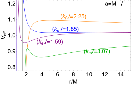
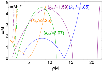
Figure 7: Case $a=M$. Effective potentials and tori orbiting BHs in perfect fluid dark matter (PFDM) of Eq. (14), for different values of the parameter $k\in]-7.18M,2M[$, describing the PFDM intensity and fluid specific angular momentum $\ell$ signed on the curves. Co-rotating $\ell^{-}=\ell>0$ cases are represented. Values $\mathbf{k_{6}}$ of Eq. (17) are considered. For $k=0$ the line element describes the extreme Kerr BH geometry. There is $r=\sqrt{x^{2}+y^{2}}$ and $\sigma=y^{2}/(x^{2}+y^{2})$, where $\sigma\equiv\sin^{2}\theta$.

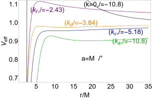
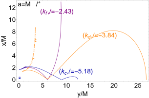
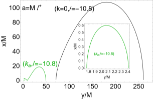
Figure 8: Case $a=M$. Effective potentials and tori orbiting BHs in perfect fluid dark matter (PFDM) of Eq. (14), for different values of the parameter $k\in]-7.18M,2M[$, describing the PFDM intensity and fluid specific angular momentum $\ell$, signed on the curves. Counter-rotating $\ell^{+}=\ell<0$ cases are represented. Values $\mathbf{k_{6}}$ of Eq. (17) are considered. For $k=0$ the line element describes the extreme Kerr BH geometry. Inside plot in the right panel is an enlarged view of the inner green torus. There is $r=\sqrt{x^{2}+y^{2}}$ and $\sigma=y^{2}/(x^{2}+y^{2})$, where $\sigma\equiv\sin^{2}\theta$.

In general DM influence manifests also with the existence of extremely large cusped tori located considerably far from the central singularity as clear comparing the geodesic structures in Figs (1) and Figs (3). In some cases, as clear from Figs (7), there are double configurations at equal $\ell$ (purple and blue curves of Figs (7) and green curve of Figs (8)), with considerable larger tori with respect to the case in absence of dark matter. Furthermore we note the presence of outer cusps (blue curve in Figs (7)) or possibly the emergence of double cusps also in presence of BH solutions, where the co-rotating marginally stable orbit shows some remarkable peculiarities at $k\geq k_{e}$ for $a=M$ and $k\in[k_{d},k_{e}]$ for $a=0$.

The inter-disk cusp (see also Figs (7)) can evolve, following the change in one or two of the tori parameters $(\ell,K)$ in an inner cusp followed by an inner configuration (as the green curve in Figs (8)) or two separated configurations (as the purple curve in Figs (7)). For $k=k_{e}$, in the case $a=M$, there are no horizons consequently the geometry, although is not over-spinning, can be considered a naked singularity, and the green curve in Figs (8) can be seen as a typical double configuration characterizing certain NS geometries. Also the presence of excretion cusps could be a DM indicator. Notably these features are usually read as tracers for the possible NSs observations, emerging as consequences of the repulsive gravity effects characterizing NSs solutions, and in this sense the Kerr BH immersed in PFDM could be a "mimicker" of super-spinars solutions.

III.2 Cold and scalar field dark matter

In this section we consider a spinning BH in scalar field dark matter (SFDM), addressed in Sec. (III.2.1) and in cold dark matter (CDM), considered in Sec. (III.2.2)–see for example [8, 9].

III.2.1 Scalar field dark matter (SFDM)

There is

$$g_{tt}=-\left[1-\frac{{2Mr}+r^{2}(1-\xi_{SFDM})}{\Sigma}\right],\quad g_{t\phi}=-\frac{a\sigma\left[{2Mr}+r^{2}(1-\xi_{SFDM})\right]}{\Sigma},\quad g_{\phi\phi}\equiv\frac{\sigma\left[\left(a^{2}+r^{2}\right)^{2}-a^{2}\sigma\Delta_{SFDM}\right]}{\Sigma}$$

$$g_{rr}\equiv\frac{\Sigma}{\Delta_{SFDM}},\quad g_{\theta\theta}=\Sigma$$ (18)

where

$$\Delta_{SFDM}\equiv a^{2}-{2Mr}+r^{2}\xi_{SFDM}\quad\mbox{and}\quad\xi_{SFDM}\equiv\exp\left[-\frac{8\rho_{c}R^{2}\sin\left(\frac{\pi r}{R}\right)}{\frac{\pi(\pi r)}{R}}\right].$$ (19)

The metric components satisfy the asymptotically flatness condition, and the fluid potential is well defined at infinity ($r\to+\infty$), where $V_{eff}=1$. We introduce the quantity $k:\rho_{c}={k}/{R^{3}}$. Here $\rho_{c}$ is the central density and $R$ is the radius at which the pressure and density are zero (where $\rho_{c}=0$ the metric reduces to the Kerr solution). The Kerr limit occurs for $k\to 0$ or $R\to+\infty$. The zeros of $\Delta_{SFDM}$ distinguish the metric singularities $r_{\pm}$ (SFDM deformed horizons), while the zeros of $g_{tt}$ define a deformation of the Kerr ergosurfaces $r_{\epsilon}^{\pm}$ , which can be found by solving the equation $a=a_{\pm}$ and $a=a_{\epsilon}^{\pm}$ respectively, where

$$a_{\pm}\equiv\sqrt{r\left(2M-r\xi_{sfdm}^{-1}\right)},\quad a_{\epsilon}^{\pm}\equiv\frac{a_{\pm}}{\sqrt{1-\sigma}}\quad\mbox{with}\quad\xi_{sfdm}\equiv e^{\frac{8k\sin\left(\frac{\pi r}{R}\right)}{\pi^{2}r}}.$$ (20)

In accordance with the study of the BHs horizons in Figs (9) we explore the following two cases:

$$\mathcal{F}_{p}\equiv\{k_{p}\to 1000M,R_{p}\to 1200M\},\quad\mathcal{F}_{g}\equiv\{k_{g}\to 20000M,R_{g}\to 120000M\},$$ (21)

(see Figs (9)).

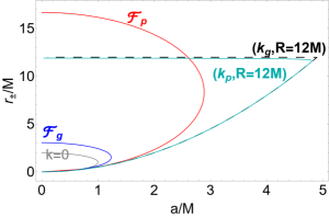
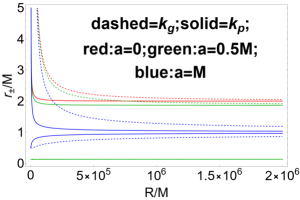
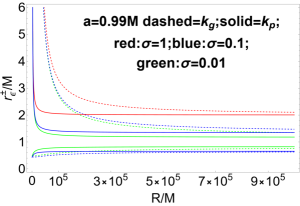
Figure 9: Horizons and ergosurfaces of BHs geometries in scalar field dark matter (SFDM) of Eq. (19). Parameters $\mathcal{F}_{p}$ and $\mathcal{F}_{g}$ are defined in Eqs (21). The case $k=0$ corresponds to Kerr or Schwarzchild geometries. Left panel shows the BH horizons $r_{\pm}$ as functions of $a/M$ for different DM parameters $(k,R)$. Gray curve is the Kerr BH horizons. Center panel: horizons radii $r_{\pm}$ as functions of the DM parameter $R$, for different $k$ and spin $a$, red curve, for $a=0$, is the static limiting case and $a=M$ is the blue curve, $a=0.5M$ is the green curve. Dashed curves correspond to $k_{g}$ and solid curves to $k_{p}$. Right panel shows the ergosurfaces as functions of $R/M$ for different $k/M$, for spin $a=0.99M$ and different planes $\sigma\equiv\sin^{2}\theta$, $\sigma=1$ (red curve) is the equatorial plane, green curve is $\sigma=0.01$, blue curve is $\sigma=0.1$, dashed curves correspond to $k_{g}$ and solid curves to $k_{p}$ defined in Eqs (21).

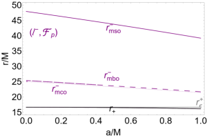
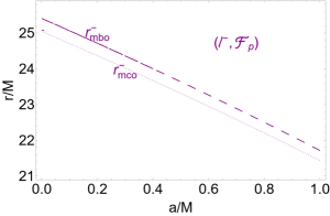
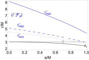
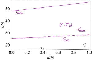
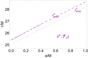
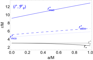
Figure 10: Geodesic equatorial structure of scalar field dark matter (SFDM) geometry of Eq. (19). Upper (bottom) panels show the situation for co-rotating (counter-rotating) fluids with $\ell^{-}$ ($\ell^{+}$) for parameters $\mathcal{F}_{p}$ (purple curves) and $\mathcal{F}_{g}$ (blue curves), defined in Eqs (21). Radius $r_{+}$ (black curve) is the outer horizon, $r_{\epsilon}^{+}$ (gray curve) is the outer ergosurface on the equatorial plane, $mso$ (solid purple and blue curves) is for marginally stable orbit, $mbo$ (dashed curves) is for the marginally bounded orbits, $mco$ (dotted curves) is for the marginally circular orbits. The correspondent Kerr geodesic structure is in Figs (1). Center panels are close-up views of the left panels.

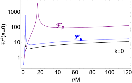
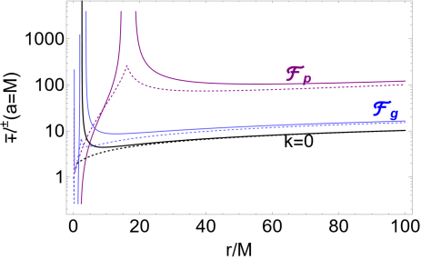
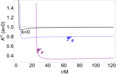
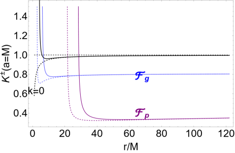
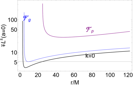
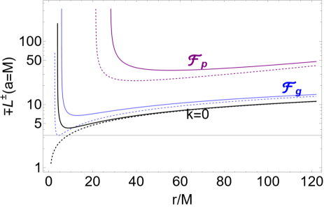
Figure 11: Fluid specific angular momentum $\ell^{\pm}$, energy parameter $K^{\pm}$ and (test particles) Keplerian angular momentum $\mathcal{L}^{\pm}$ as function of $r/M$ for co-rotating $(-)$ and counter-rotating $(+)$ fluids and different scalar field dark matter (SFDM) parameters $\mathcal{F}_{p}$ (purple) and $\mathcal{F}_{g}$ (blue), defined in Eqs (21). The value $k=0$ corresponds to the Schwarzschild ($a=0$) extreme Kerr BH case ($a=M$). The columns are $a=0$ (left) and $a=M$ (right), and rows are for $\ell$ as function of $r$ (top), $K$ as function of $r$ (middle), $\mathcal{L}$ as function of $r$ (bottom).

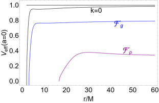
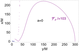
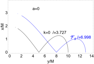
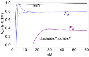
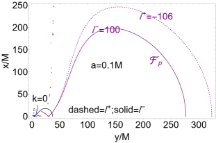
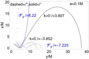
Figure 12: Fluids effective potentials (left panels) and tori (center and right panels) orbiting in scalar field dark matter (SFDM) geometry of Eq. (19), with parameters $\mathcal{F}_{p}$ (purple curves) and $\mathcal{F}_{g}$ (blue curves), defined in Eqs (21). The geodesic structure is in Figs (10). Rows are $a=0$ (top), $a=0.1M$ (middle), $a=0.9M$ (bottom). Black curves for $k=0$ are the configurations for the case of Schwarzschild and Kerr spacetimes in absence of DM. Tori are shown in the correspondent colors association relative to the effective potentials. Fluid specific angular momenta $\ell^{+}$ (dashed curves) and $\ell^{-}$ (solid curves) are signed close to each tori surface (center and right panels). Right panels are an enlarged view of the center panels in the region close to the central attractor. (The integration is in the entire orbital range). There is $r=\sqrt{x^{2}+y^{2}}$ and $\sigma=y^{2}/(x^{2}+y^{2})$, where $\sigma\equiv\sin^{2}\theta$.

However, as clear from Figs (9), BH horizons exist also for $a>M$.

The geometry circular geodesic structure is shown in Figs (10) for the parameter $\mathcal{F}_{g}$ and $\mathcal{F}_{p}$, emphasizing the differences for the cases $(k_{p},R_{p})$ and $(k_{g},R_{g})$ and the Kerr geometry circular structure of Figs (1). The orbital range locating the proto-jets cusps, bounded by the radii $r_{mbo}^{\pm}$ and $r_{mco}^{\pm}$, for fluids specific angular momentum $\ell=\ell^{\pm}$ is very narrow, and in general the geodesic structure is shifted considerably outwardly with the respect to the Kerr geometry geodesic radii. Therefore the range for the location of the accreting disks inner edges is considerably larger that the proto-jets cusp range, constituting possibly a constraint on the formation of proto-jets and tori with large angular momentum magnitude. We note also that in the co-rotating case, for $a\in]0,M]$, and for $\mathcal{F}_{p}$ differently from the Kerr case in absence of DM, radii are located out of the ergoregion (and partially for $\mathcal{F}_{g}$), this could imply a significant difference in the Lense-Thirring effects in presence of DM. (There can be however over-spinning BHs (with $a>M$) where these effects could be present). Differently from the PFDM case, qualitatively the geodesic structure is not differentiated with the respect to the case in absence of SFDM for co-rotating or counter-rotating fluids, and for static attractors ($a=0$) and spinning attractors ($a\in]0,M]$) with SFDM.

We analyse below the case of the static attractor i.e. $a=0$, having as limit in the vacuum the Schwarzschild metric, we then studied the influence of the central attractor spin combined with dark matter effects, considering the case $a=M$, corresponding to the DM deformation of the vacuum solution (i.e. in absence of DM) of the extreme Kerr BH, and the case of the slowly spinning attractor having $a=0.1M$. More specifically:

–The static attractor ($a=0$)

In Figs (11) the fluid specific angular momentum $\ell^{\pm}$, tori energy parameter $K^{\pm}$ and (test particles) Keplerian angular momentum $\mathcal{L}^{\pm}$ are shown as functions of $r/M$ for co-rotating and counter-rotating fluids, at different spins and SFDM parameters, compared to the case $k=0$ corresponding to the Schwarzschild geometry. Tori and effective potentials are in Figs (12).

–The spinning attractors ($a=M$ and $a=0.1M$)

We restrict our analysis to $a=M$ and $a=0.1M$, studying the cusped tori limiting the closed configurations, regulated by the effective potential function. In Figs (11), there are the fluid specific angular momentum $\ell^{\pm}$, energy parameter $K^{\pm}$ and (test particles) Keplerian angular momentum $\mathcal{L}^{\pm}$ as function of $r/M$ for co-rotating and counter-rotating fluids, different spins and SFDM parameters of Eq. (19), with respect to the Kerr vacuum cases. In Figs (12) are the fluids effective potentials and tori compared to the case of Kerr in absence of DM.

From Figs (11) we note that, within this parameter choice, differently from the case in absence of DM, the fluids energy function can not converge to $1$ for large values of $r$. In Figs (11) the fluid specific angular momentum distribution, compared to the distribution on the geometry in absence of DM, the associated $K$ energy parameter and the Keplerian (test particle) angular momentum $\mathcal{L}^{\pm}\equiv\ell^{\pm}K^{\pm}$ are shown. From Figs (9) it is clear how the horizon curves in the plane $a-M$ are larger and shifted outwardly with respect to the Kerr BH case, constituting a discriminant for the SFDM model and, for some values of the DM parameters, the BH horizons disappear giving rise to a "DM–induced" NS.

Large tori orbiting SFDM spinning BHs are shown in Figs (12) as, for example, the purple surface for the case $a=0$ (from the tori effective potentials we can also note how the tori $K$ parameter for tori orbiting in SFDM are generally considerably lower than the $K$ parameter in absence of DM).

This feature of the DM model could also be an indication that such extremely huge tori are actually not formed and similarly the back-reaction on the metric is a predominant factor in these configurations, where self-gravity becomes a determinant factor in the tori equilibrium.

III.2.2 Cold Dark Matter (CDM)

The metric components read

$$g_{tt}=-\left[1-\frac{{2Mr}-\xi_{CDM}+r^{2}}{\Sigma}\right],\quad g_{t\phi}=-\frac{a\sigma\left[{2Mr}-\xi_{CDM}+r^{2}\right]}{\Sigma},\quad g_{\phi\phi}\equiv\frac{\sigma\left[\left(a^{2}+r^{2}\right)^{2}-a^{2}\sigma\Delta_{CDM}\right]}{\Sigma};$$

$$g_{rr}\equiv\frac{\Sigma}{\Delta_{CDM}},\quad g_{\theta\theta}=\Sigma$$ (22)

where

$$\Delta_{CDM}\equiv a^{2}-{2Mr}+\xi_{CDM}\quad\mbox{and}\quad\xi_{CDM}\equiv r^{2}\left(\frac{r}{R}+1\right)^{-\frac{8\pi\rho_{c}R^{3}}{r}}.$$ (23)

We adopt the parametrization $\rho_{c}={k}/{R^{3}}$, where $\rho_{c}$ is the density of the universe at the moment when the DM halo collapsed, $R$ is a characteristic radius. The metric is asymptotically flat and we find the Kerr limit in $k\to 0$ or $R\to+\infty$. We first consider the metric singularities, identifying the space of the parameters used in the tori analysis. The horizons $r_{\pm}$ can be written as solutions of the equation $a=a_{\pm}(CDM)$, or $R=R_{\pm}(CDM)$ or $k=k_{\pm}(CDM)$ where

$$a_{\pm}(CDM)\equiv\sqrt{r\left[2M-r\wp^{-\frac{8\pi k}{r}}\right]},\quad R_{\pm}(CDM)\equiv r\left[\frac{1}{1-\varsigma^{\frac{r}{8\pi k}}}-1\right],\quad k_{\pm}(CDM)\equiv\frac{r\log\varsigma^{-1}}{8\pi\log\wp},$$

$$\mbox{with}\quad\wp\equiv\frac{r}{R}+1,\quad\mbox{and}\quad\varsigma\equiv\frac{2rM-a^{2}}{r^{2}}.$$ (24)

The metric horizons are defined for

$$a\in]0,M]:\quad r\in\left]r_{\circledast},{r_{-}}\right[;\quad a\in[0,M]:r>{r_{+}};\quad a>M:r>r_{\circledast},\quad\mbox{where}\quad r_{\circledast}\equiv\frac{a^{2}}{2M},$$

(assuming $a>0,R>0,k>0$).

The ergosurfaces $r_{\epsilon}^{\pm}$ can be found for $\sigma\neq 1$ as solutions of the equation $a=a_{\epsilon}^{\pm}(CDM)\equiv{a_{\pm}(CDM)}/{\sqrt{1-\sigma}}$ and, on the equatorial plane $(\sigma=1)$ as solutions of $R=R_{\epsilon}^{\pm}$ or $k=k_{\epsilon}^{\pm}$ where

$$k_{\epsilon}^{\pm}\equiv\frac{r\log\frac{r}{2M}}{8\pi\log\wp}\quad\mbox{and}\quad R_{\epsilon}^{\pm}\equiv r\left[\frac{1}{1-\left(\frac{2M}{r}\right)^{\frac{r}{8\pi k}}}-1\right],$$ (25)

see Figs (13). On the equatorial plane, the outer ergosurface, independent on the spin $a$, corresponds to the metric singularity in the static ($a=0$) case–see Eqs (24).

We consider the following sets of parameters

$$\mathcal{F}_{1}\equiv\{k\to 1000M,R\to 120000M\},\quad\mathcal{F}_{2}\equiv\{k\to 100M,R\to 1200M\},\quad\mbox{and}\quad k_{(p)}\equiv 100M$$ (26)

–Figs (13).

Figure 13: Horizons $r_{\pm}$ and ergosufaces $r_{\epsilon}^{\pm}$ of the cold dark matter CDM geometry of Eqs (22). Dark matter parameters $\mathcal{F}_{1}$, $\mathcal{F}_{2}$ and $k_{(p)}$ are in Eqs (26), parameters $(k_{p},k_{g},R_{g},R_{p})$ are in Eqs (21) . Black curves, $k=0$, correspond to the Kerr horizons. There is $\sigma\equiv\sin^{2}\theta$, where $\sigma=1$ is the equatorial plane. In the bottom left panel blue curves are $a=M$, red curves are $a=0$, green curves are $a=0.5M$, dotted curves are for $k=k_{(p)}$, dashed curves are for $k=k_{g}$, solid curves are for $k=k_{p}$, black horizontal lines correspond to $k=0$ for the Kerr spacetimes. Bottom right panel shows the ergosurfaces $r_{\epsilon}^{\pm}$ as function of the dark matter parameter $R/M$ for spin $a=0.99M$ and for different planes $\sigma\in[0,1]$ and dark matter parameter $k$, where red curves correspond to $\sigma=1$, blue curves correspond to $\sigma=0.1$, brown curves to $\sigma=0.01$, dashed curves are for $k=k_{g}$, solid curves for $k=k_{p}$ and dotted curves are for $k=k_{(p)}$.

The geodesic structure for this geometry is shown in Figs (14).

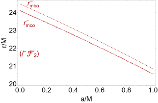
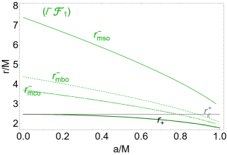
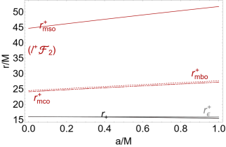
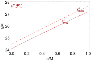
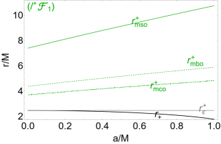
Figure 14: Geodesic equatorial structure of the cold dark matter CDM geometry of Eqs (22). Dark matter parameters $\mathcal{F}_{1}$ (green curves) and $\mathcal{F}_{2}$ (red curves) are in Eqs (26). Upper (below) panels show the structure for fluid specific angular momentum $\ell=\ell^{-}>0$ ($\ell^{+}<0$) for co-rotating (counter-rotating) fluids. Center panels are an enlarged view of the right panels, showing the marginally stable orbits ($mso$ solid curves) marginally bounded orbits ($mbo$ dashed curves) and marginally circular orbits $r_{mco}^{\pm}$ (dotted curves), where $r_{+}$ (black curves) is the outer horizon, $r_{\epsilon}^{+}$ (gray curves) is the outer ergosurface on the equatorial plane. The correspondent Kerr geodesic structure is in Figs (1).

Similarly to the SFDM model, the equatorial geodesic structure shows that for the $\mathcal{F}_{2}$ case, the range $[r_{mco}^{\pm},r_{mbo}^{\pm}]$ of the proto-jets cusp location is remarkably narrow. At $a\in]0,M]$, for co-rotating fluids, the radii for $\mathcal{F}_{1}$ ($\mathcal{F}_{2}$) do not enter (are partially contained in) the outer ergoregion.

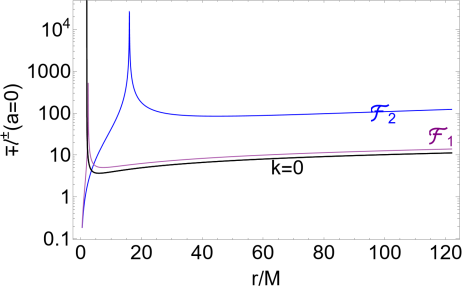
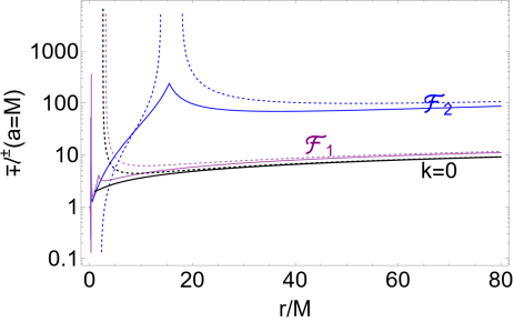
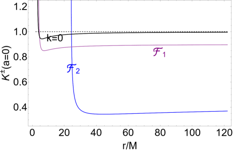
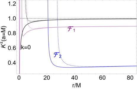
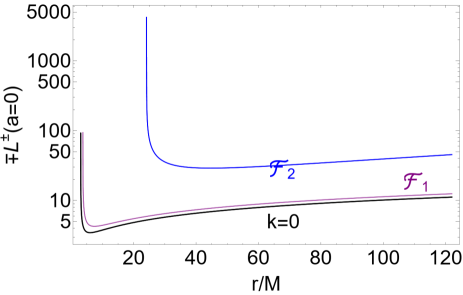
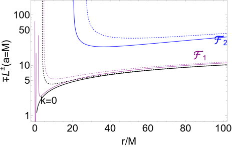
Figure 15: Fluid specific angular momentum $\ell^{\pm}$ (upper row), energy parameter $K^{\pm}$ (middle row) and (test particles) Keplerian angular momentum $\mathcal{L}^{\pm}$ (bottom row) as function of $r/M$ for co-rotating and counter-rotating fluids, different cold dark matter CDM parameters of Eqs (22). Dark matter parameters $\mathcal{F}_{1}$ (purple curves) and $\mathcal{F}_{2}$ (blue curves) are in Eqs (26). The columns are $a=0$ (left) and $a=M$ (right). Kerr and Schwarzschild case are the black curves for $k=0$.

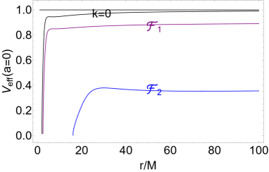
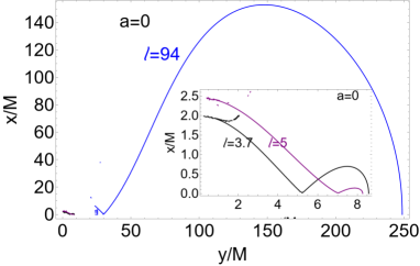
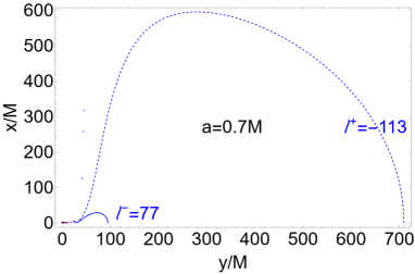
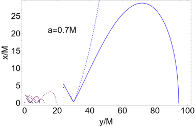
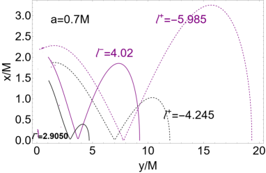
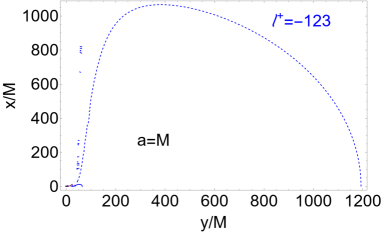
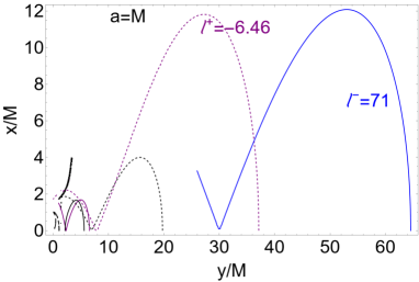
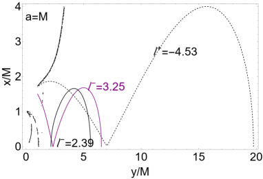
Figure 16: Effective potential and tori of the cold dark matter CDM geometry. Dark matter parameters $\mathcal{F}_{1}$ (purple curves) and $\mathcal{F}_{2}$ (blue curves) are in Eqs (26). Rows are $a=0$ (top line), $a=0.7M$ (top second and third lines), $a=M$ (top fourth and fifth lines). Black curves for $k=0$ are the configurations for the case of Schwarzschild and Kerr spacetimes in absence of DM. Tori are shown in the correspondent colors association relative to the effective potentials. Fluid specific angular momenta $\ell^{+}$ (dashed curves) and $\ell^{-}$ (solid curves) are signed close to each tori surface. Regions close to the central attractor are also shown in enlarged views panels. There is $r=\sqrt{x^{2}+y^{2}}$ and $\sigma=y^{2}/(x^{2}+y^{2})$, where $\sigma\equiv\sin^{2}\theta$.

We have analyzed the static and spinning attractors as follows:

–The static attractor ($a=0$)

The fluid specific angular momentum $\ell^{\pm}$, energy parameter $K^{\pm}$ and (test particles) Keplerian angular momentum $\mathcal{L}^{\pm}$ as function of $r/M$, and CDM parameters $\mathcal{F}_{1}$ and $\mathcal{F}_{2}$ are in Figs (15), compared to the Schwarzschild case. The effective potential and tori are shown in Figs (16) compared with the Schwarzschild case.

–The spinning attractor ($a\neq 0$)

Fluid specific angular momentum $\ell^{\pm}$, energy parameter $K^{\pm}$ and (test particles) Keplerian angular momentum $\mathcal{L}^{\pm}$ as function of $r/M$ are represented in Figs (15) for co-rotating and counter-rotating fluids, different spins and CDM parameters $\mathcal{F}_{1}$ in comparison with the extreme Kerr BH case in absence of DM. Effective potential and tori for CDM parameters $\mathcal{F}_{1}$ and $\mathcal{F}_{2}$ are in Figs (16), for $a=M$ and $a=0.7M$ in Figs (16), for fluid specific angular momentum $\ell=\ell^{-}>0$ ($\ell^{+}<0$) for co-rotating (counter-rotating) fluids, compared with the case in the vacuum Kerr geometry

It can be proved that, in all the cases considered, the limit $K\to 1$ for large $r$ holds, where $\mathcal{L}^{\pm}\equiv\ell^{\pm}K^{\pm}$. Large tori orbiting CDM spinning BHs are shown in Figs (16) as, for example, the blue surface for the case $a=0$, dashed -blue curve for $a=0.7M$ and $a=M$ (similarly to the SFDM case, the tori $K$ parameter for tori orbiting in CDM are generally considerably lower than the $K$ parameter in absence of DM).

From Figs (16) we note, as for SFDM, the presence of larger cusped tori located far from the central spinning attractor, distinguishing the DM deformed geometry from the Kerr case.

IV Discussion and Final Remarks

In DM models considered here there are NS solutions, solutions with one horizon and two horizons, according to the DM parameters. There are also BH spacetime solutions with horizons at $a>M$ or NSs for $a<M$. The geodesic structure regulating the accretion physics and the tori location around the central spinning attractor can be shifted considerably outwardly with the respect to the Kerr geometry. DM effects mimic Kerr attactors with altered spin to mass ratio $a/M$. For example, in all the models presented, the DM affects the disk inner edge which is a tracer of the $a/M$ in the Kerr geometry. The presence of an excretion cusp, double cusps, or double tori, which are also typical of Kerr NSs solutions, could indicate the presence of DM. Consequently DM affects BH horizon physics, considering DM (models) as NSs mimickers, or vice versa DM (models) as BHs mimickers for super-spinars (cosmological) solutions. DM could also affect the jet emission. The orbital range locating the proto-jets cusps can be also very small, as discussed in Sec. (III.2.1) for SFDM and in Sec. (III.2.2) for CDM. The open cusped solutions (constraining also the jet emission) are very different from their counterparts in the Kerr spacetime in absence of DM. In general DM manifests also with the existence of extremely large cusped tori orbiting very far from the central singularity. From Figs (12) we see the large dimensions of the cusped tori orbiting SFDM spinning BHs. The equilibrium of these tori may be hugely affected by the their self-gravity.

In all DM models considered here, however, DM affects the geometric and causality properties, while there is no coupling with ordinary matter (nor an hypothetical accretion disk consisting of dark matter in orbit), considering gravity modified by the effects of the dark matter–see also [78]. We addressed three models, drawing qualitative and comparative considerations, ruling out some solutions and tracing some common patterns. We have taken as a selection criterion in the space of the metric parameters the observation that there are two expected regimes, where there is a fully modified geometry, qualitatively divergent with respect to the general relativistic onset, as a strongly different horizons structures compared to the reference Kerr solution, and the second scenarios consisting in an appreciable quantitative deformation of the orbiting structures, but not a qualitatively significant change of the background geometry defined by the spinning BH. The current methods of measuring and identifying BHs are based also on the physics of accretion, being related to the accretion disk inner edge, which we prove to be distorted by the DM treated, in the metric models considered here, as a background deformation.

Spherically symmetric black hole solutions in PFDM have been considered to be adapted to the observed asymptotically flat rotation velocity in spiral galaxies and a possible interaction between the DM halo and central BH has been differently theorized. However it has been supposed that SMBHs could enhance the DM density significantly. The results of our analysis prove accretion to be a good indicator of the divergences induced by the DM presence and the study of the accretion disks in DM models to represent a valid DM models discriminant. The tori dimensions provide an indication of the possible effects of DM for the energetics associated with the physics of accretion around BHs. In the P-D models for example, the thickness of the accretion throat (opening of the cusp for tori with specific fluid angular momentum in L1 with $K\in]K_{\times},1[$) determines (in the assumptions of vanishing pressure at the inner edge), many characteristics of tori energetics such as mass accretion rates and cusp luminosity, the rate of the thermal-energy carried at the cusp, the mass flow rate through the cusp (i.e., mass loss accretion rate), the fraction of energy produced inside the flow and not radiated through the surface but swallowed by central BH, mass-flux, the enthalpy-flux (related to the temperature parameter), depending also on the EoS, as the polytropic index and constant. It has been shown in [73, 80] that the maximum of flow thickness and the maximum amount of matter swallowed by the central BH is determined by the attractor spin–mass ratio only, being defined by the location of the marginally stable circular orbit, and therefore DM influences on the tori dimension and the marginally stable orbits in these models can be searched in a variation of the central BH energetics [64, 65, 80].

It should be emphasized then that since DM-BHs can exhibit features associated with Kerr NSs, it has implications on cosmic censorship, in the fact that observing a compact object with such tracers (excretion cusp, double cusps, double tori) would not require the breaking of cosmic censorship (viewing a Kerr NSs), but instead could mean one is observing a BH surrounded by DM. Finally in this work we developed a comparative analysis of accretion disks in different dark matter models while we reserve the in-depth explorations of different DM parametric values for future analysis.

References

- [1] P. E. Mancera Piña, F. Fraternali, T. Oosterloo, et al., MNRAS, 512, 3230 (2022).
- [2] P. E. Mancera Pina et al., ApJL, 883, L33 (2019).
- [3] E. Belbruno, J. Green, MNRAS, 510, 4, 5154-5163 (2022).
- [4] X. Hou, Z. Xu and J. Wang, JCAP, 12, 04 (2018).
- [5] F. Rahaman, K.K. Nandi, A. Bhadra, et al, Physics Letters B, 694, 10–15 (2010).
- [6] Z. Xu, X. Hou and J. Wang, Class. Quantum Grav. 35, 115003 (2018).
- [7] A. Das et al. Class. Quantum Grav., 38, 065015 (2021).
- [8] Z. Xu, X. Hou, X. Gonga, J. Wanga, JCAP,09, 038 (2018).
- [9] X. Hou, Z. Xu, M. Zhou, and J. Wang, JCAP,07, 015 (2018).
- [10] S. Shaymatov, D. Malafarina, B. Ahmedov, Physics of the Dark Universe, 34, 100891 (2021).
- [11] Z. Stuchlik, BAIC 34, 129, (1983).
- [12] Z. Stuchlík & S. Hledík, Physical Review D, 60, 044006 (1999).
- [13] Z. Stuchlík, M. Kološ, J. Kovář, Slaný et al., Univ, 6, 26 (2020).
- [14] Z. Stuchlík, S. Hledík, CQGra, 17, 4541 (2000).
- [15] Z. Stuchlík, MPLA, 20, 561 (2005).
- [16] M. Khodadi, R. Pourkhodabakhshi, Physics Letters B, 823, 136775 (2021).
- [17] B. Toshmatov, Z. Stuchlik, B. Ahmedov, Eur. Phys. J. Plus, 132, 98 (2017).
- [18] H. Kim, B. Lee, W. Lee, and Y. Lee, Physcal Review D, 101, 064067, (2020).
- [19] B. Cuadros-Melgar, R. D. B. Fontana, J. de Oliveira, Physical Review D, 104, 104039 (2021).
- [20] M. Li and K. Yang, Physical Review D 86, 123015, (2012).
- [21] Z. Stuchlík, J. Schee, CQGra, 30, 075012 (2013).
- [22] Z. Stuchlik, BAICz, 31, 129 (1980).
- [23] M. Blaschke, Z. Stuchlík, PhRvD, 94, 086006 (2016).
- [24] Z. Stuchlík, S. Hledík, K. Truparová, CQGra, 28, 155017 (2011).
- [25] R. Abbott et al, arXiv:2111.15507v1 [astro-ph.HE].
- [26] D. Traykova et al. Phys. Rev. D 104, 103014 (2021)
- [27] K. Clough, P. G. Ferreira, and M. Lagos, Phys. Rev. D 100, 063014, (2019).
- [28] J. Bamber, K. Clough, P. G. Ferreira, L. Hui, and M. Lagos, Phys. Rev. D 103, 044059 (2021).
- [29] H. Davoudias, P. B. Denton and J. Gehrlein Physical Review Letters 128, 081101 (2022).
- [30] L. E. Padilla, T. Rindler-Daller, P. R. Shapiro, et al.Phys. Rev. D 103, 063012 (2021).
- [31] J. Bamber, K. Clough, P. G. Ferreira, L. Hui, and M. Lagos, Phys. Rev. D 103, 044059, (2021).
- [32] K. Jusufi Phys. Rev. D ,101, 084055 (2020).
- [33] T. Lacroix, M. Karami, A. E. Broderick, J. Silk, C. Boehm Physical Review D 96, 063008 (2017).
- [34] K. Jusufi, M. Jamil, T. Zhu, Eur. Phys. J. C, 80, 354 (2020).
- [35] K. Jusufi, M. Jamil, P. Salucci, T. Zhu, and S. Haroon, Physical Review D 100, 044012 (2019).
- [36] F. Atamurotov et al. Class. Quantum Grav. 39, 025014 (2022).
- [37] A. Das et al., Phys. Rev. Lett. 128, 021101 (2022).
- [38] T. S. Li, A. P. Ji, A. B. Pace, et al., Astrophys. J. , 928, 30 (2022).
- [39] R. P. Naidu, C. Conroy, A. Bonaca, et al., Astrophys. J. , 923, 92 (2021).
- [40] N. Cappelluti, G. Hasinger, P. Natarajan, ApJ, 926, 205 (2022).
- [41] S. Basak et al,ApJ Lett., 926, L28 (2022).
- [42] C. Smorra, Y. V. Stadnik, P. E. Blessing,et al. Nature, 575, 7782, 310-314 (2019).
- [43] S. Afach, B.C. Buchler, D. Budker, et al. Nat. Phys. 17, 1396–1401 (2021).
- [44] A. Gomez-Valent, Z. Zheng, L. Amendola, et al. Phys. Rev. D, 104, 083536 (2021).
- [45] Z. Stuchlí, S. Hledík, J. Novotný, PhRvD, 94, 103513 (2016).
- [46] M. Kozłowski, M. Jaroszyński, M. A. Abramowicz Astron. Astrophys., 63, 209 (1998).
- [47] M. A. Abramowicz,M. Jaroszyński, M. Sikora Astron. Astrophys, 63, 221 (1978).
- [48] M. Jaroszynski, M. A.Abramowicz, B. Paczynski, Acta Astron., 30, 1 (1980).
- [49] D. Pugliese, G. Montani & M. G. Bernardini, Mon. Not. R. Astron. Soc., 428 (2), 952 (2013).
- [50] D. Pugliese& G. Montani, Europhys. Lett., 101, 19001 (2013).
- [51] I. V. Igumenshchev, M. A. Abramowicz, Astrophys. J. Suppl.,130, 463 (2000).
- [52] R. Shafee, J. C McKinney, R. Narayan, et al. Astrophys. J. , 687, L25 (2008).
- [53] P. C. Fragile, O. M. Blaes, P. Anninois, J. D. Salmonson, Astrophys. J. , 668, 417-429 (2007).
- [54] J-P. De Villiers,& J. F. Hawley, Astrophys. J. , 577, 866 (2002).
- [55] Q. Lei, M. A. Abramowicz, P. C. Fragile, et al., A&A., 498, 471 (2008).
- [56] M. A. Abramowicz, arXiv:astro-ph/0812.3924 (2008).
- [57] J. A. Font& F. Daigne, Astrophys. J. , 581, L23–L26 (2002).
- [58] M. A. Abramowicz& P.C. Fragile, Living Rev. Relativity, 16, 1 (2013).
- [59] D. Pugliese and G. Montani, Phys. Rev. D 91, 8, 083011 (2015).
- [60] B. Paczyński, Acta Astron., 30, 4 (1980).
- [61] J. A. Font, Living Rev. Relat., 6, 4 (2003).
- [62] M. Kozłowski, M. Jaroszyński, M. A. Abramowicz, Astron. Astrophys., 63, 209 (1998).
- [63] M. A. Abramowicz, M. Calvani, L. Nobili, Astrophys. J., 242, 772 (1980).
- [64] M. A. Abramowicz, Astronomical Society of Japan, 37, 4, 727-734 (1985).
- [65] D. Pugliese&Z. Stuchlik , Eur. Phys. J. C 79 4, 288, (2019).
- [66] D. Pugliese & Z. Stuchlík,Class. Quant. Grav. 35, 18, 185008 (2018).
- [67] Z. Stuchlik, BAICz, 32, 68 (1981).
- [68] D. Pugliese, H. Quevedo and R. Ruffini, Phys. Rev. D, 84, 044030 (2011).
- [69] K. Adamek, Z. Stuchlik, CQGra, 30, 205007, (2013).
- [70] P. Slaný, Z. Stuchlík, CQGra, 22, 3623, (2005).
- [71] D. Pugliese&Z. Stuchlík, Astrophys. J.s, 221, 2, 25 (2015).
- [72] D. Pugliese, G. Montani, Gen. Rel. Grav, 53,5,51, (2021).
- [73] D. Pugliese, Z. Stuchlik, submitted 2022.
- [74] D. Pugliese&Z.Stuchlík, Astrophys. J.s, 223, 2, 27 (2016).
- [75] D. Pugliese & Z. Stuchlík, Class. Quant. Grav. 35,10, 105005 (2018).
- [76] D. Pugliese, Z. Stuchlik, PASJ,73, 5, 1333-1366, (2021).
- [77] D. Pugliese, Z. Stuchlik, PASJ- 73, 6, 1497-1539 (2021)
- [78] E. Kurmanov, K. Boshkayev, R. Giambo, et al.Astrophys. J. , 925, 210, (2022)
- [79] L. Sadeghian, F. Ferrer and C.M. Will, Phys. Rev. D 88, 063522 (2013).
- [80] D. Pugliese, Z. Stuchlik, MNRAS, 512, 4, 5895–5926, (2022).
- [81] R. H. Boyer, Proc. R. Soc. London A, 311, 245 (1969).
- [82] O. Porth, H. Olivares, Y. Mizuno, Z. Younsi, et al.arXiv:1611.09720 [gr-qc] (2017).