Deep Bayesian Future Fusion for
Self-Supervised, High-Resolution, Off-Road Mapping

Abstract

The limited sensing resolution of resource-constrained off-road vehicles poses significant challenges towards reliable off-road autonomy. To overcome this limitation, we propose a general framework based on fusing the future information (i.e. future fusion) for self-supervision. Recent approaches exploit this future information alongside the hand-crafted heuristics to directly supervise the targeted downstream tasks (e.g. traversability estimation). However, in this paper, we opt for a more general line of development – time-efficient completion of the highest resolution (i.e. $2$cm per pixel) BEV map in a self-supervised manner via future fusion, which can be used for any downstream tasks for better longer range prediction. To this end, first, we create a high-resolution future-fusion dataset containing pairs of (RGB / height) raw sparse and noisy inputs and map-based dense labels. Next, to accommodate the noise and sparsity of the sensory information, especially in the distal regions, we design an efficient realization of the Bayes filter onto the vanilla convolutional network via the recurrent mechanism. Equipped with the ideas from SOTA generative models, our Bayesian structure effectively predicts high-quality BEV maps in the distal regions. Extensive evaluation on both the quality of completion and downstream task on our future-fusion dataset demonstrates the potential of our approach.

I Introduction

Figure 2: Sample BEV images (cropped) showing the same region with different pixel resolutions – $2$cm used in this work and $20$cm which is the finest in recent literature [1]. The difference in the perceptual quality for a typical off-road terrain is evident.

High-resolution maps are critical for off-road navigation due to the delicacy of the off-road terrains, including but not limited to uneven changes in elevation, vegetation, and other intricate geological features, such as sand dunes, gravels, muds, etc. Thus, high-resolution, considerably long-range maps enable the off-road agent in identifying diverse obstacles to avoid getting stuck while traversing the challenging terrains. In other words, detailed maps facilitate the agent to plan for the optimal paths more effectively by analyzing the traversability (i.e. terrain roughness, gradients, vegetation density, etc.) in sufficient detail.

Recent works in off-road autonomy attempt to address the mapping problem with the finest BEV resolution of 20–40cm [1, 2]. This tentative bias towards coarser granularity is partly due to the limited sensing range and precision of the off-road autonomy stack compared to their commercially available civilian counterparts. For instance, the baseline for the stereo rig in KITTI [3] is approximately 54cm but only 21cm for the Multisense S21 installed in the Yamaha All-Terrain Vehicle (ATV) used in TartanDrive [4]. However, as shown in Figure 2, this level of resolution significantly smooth out the spatial perception of the terrain, eventually blurring out the ability of the models to reason in finer detail whenever necessary.

Therefore, in this paper, we focus on generating dense BEV maps given the sparse BEV map as input (Figure 1) at a resolution of 2cm – significantly higher than ever encountered in the off-road literature. Following the recent advances of the GPU infrastructures, we believe that this level of resolution is going to be mainstream in the next few years. Also, as noted above, the sensing restrictions already poses significant challenges towards this goal. More specifically, both the noise and the level of sparsity increases significantly with the distance of the point from the ego-vehicle (Figure 1). Thus, the available input map accumulated from the previous history provide an initial estimate per point that requires further refinement to a variable degree depending upon the point-wise ego distance. Consequently, this nonlinear refinement task imposes additional challenges on top of the standard map completion or filling for our case.

To solve this variable refinement and densification problem in the context of off-road navigation, first we create a dataset of input/label pairs containing both stereo RGB and LiDAR height attributes. In this regard, we devise a practical heterogeneous implementation (CPU/GPU) of registering over billions of points comprising the complete trajectory maps and then generating BEV input/label maps per frame at a pragmatically fast pace.

On the modeling side, existing literature predict the downstream features directly, such as estimating the {traversability, elevation} [1] or {semantic labels, elevation} [2] from the input and label pairs. Instead, we aim to generate better quality BEV maps from noisy and sparse input up to the present time stamp (Figure 1). In this regard, our self-supervised map completion problem is generalized regardless of the choice of downstream tasks. In fact, our completed maps can be employed for better performance on any other tasks down the line. With that in mind, we devised a computationally efficient desne map completion module. Moreover, to address the issue of variable pixel-wise refinement and completion at the same time, we materialize the Bayes filter mechanism [5] into our vanilla model with negligible increase in inference time.

Our Bayesian model trained with the recent advances in generative modeling [6, 7] can predict (i.e. complete and refine) the input maps with high-fidelity (Figure 1, 6). In addition, we demonstrate the efficacy of both the generated labels and our predictions on the downstream task of predicting vehicle dynamics [8].

In summary, our contributions are as follows:

• We propose a scalable data-generation protocol for self-supervised, dense map completion. With that, we generate a large-scale dataset comprising high-resolution (i.e. 2 cm) (raw input / dense label) pairs for RGB and height by fusing the future map information (i.e. future-fusion).

• We refine and complete the input BEV maps with an efficient convolutional-recurrent mechanism, which is a realization of the well-known Bayes filter [5]. We call this framework Deep Bayesian Future-Fusion (DBFF).

• We validate the DBFF map on the downstream task of vehicle dynamics prediction for offroad navigation, and demonstrate more than 20% relative improvement.

II Related Works

Irregular hole-filling and image inpainting: Recent works on image inpainting and depth completion address the irregular shaped holes needed to be filled with different forms of normalized variants of the standard convolution operation [9, 10, 11]. However, unlike plain convolutions, these customized convolution operations equipped with various normalization tricks are quite difficult to accelerate via matrix multiplication [12]. Moreover, based on a pilot study, we find no significant improvement in terms of reconstruction error for our map completion task. CRA [13] proposes a low-resolution hole-filling followed by adversarial low to high resolution transfer. For our task, where the input comprises salt and pepper like holes, the pooled low resolution images destroy the texture distributions of the images and thus take the low resolution transfer task severely out-of-distribution, which we empirically find difficult to recover in the later stage.

We purposely omit recent advances based on the combination of diffusion models and transformers [14, 15, 16, 17] due to their significantly higher computational and runtime complexity than modern off-road ATVs [4] can support in real time.

Point cloud forecasting: The closest subdomain to our BEV map completion task for offroad driving is point cloud forecasting [18, 19, 20, 21] where the points at future time steps are predicted from the previous scans. The spatio-temporal 3D CNN [18] predicts the future projections in 2D spherical view by stacking the scans from the past. SPF [19] utilizes a similar forecasting pipeline for detection and tracking afterward. Stochastic SPF [20] incorporates probabilistic generative modeling into SPF via temporally-conditioned latent space learning. The 4D occupancy network [21] bypasses the exact points prediction problem with an easier proxy of 4D occupancy grid forecasting. All these methods focus on various forms of representation learning than generating very high-resolution dense maps. Moreover, these methods are evaluated on the urban scenarios which are biased towards discrete objects like vehicles, pedestrians, road signs, etc. Therefore, to our knowledge, we are the first to deal with high-resolution self-supervised dense BEV map completion in the context of off-road driving.

Image-guided monocular depth completion: Another subdomain similar to our BEV RGB/height completion task is supervised monocular depth completion (MDC) [22] where the inputs are registered RGB image and sparse depth from the LiDAR point cloud and the output is the dense version of this depth map. Recent works on supervised MDC focus on the design of better multimodal fusion networks from FPV [23] and BEV [24], gradual multi-stage refinement [25], learnable attention-based propagation of spatial affinity among neighboring pixels [26], and amalgamation of convolution and SOTA transformer modules [27]. Nonetheless, supervised MDC is arguably an easier problem for a couple of reasons. First, the scale ambiguity is quite resolvable with the direct supervision from sparse depth input. Second, the vanishing point and absolute position of the objects in the image provides the network strong priors for depth estimation [28, 29, 30]. Next, predicting both the dense RGB texture and height from their sparse and somewhat undistilled counterparts like ours is a much more difficult learning problem than depth densification.

Inpainting in off-road navigation: BEVNet [31] predicts a BEV semantic map from on-board lidar data. TerrainNet [2] further extends this, consuming stereo pairs and predicting the elevation map along with the semantic map. UNRealNet [32] estimates robot-agnostic traversability features with an eye on test-time adaptation. ALTER [33] learns to approximates the dense traversability costmap in the FPV space based on geometric cues. Finally, RoadRunner [1] learns to fuse lidar and RGB information based on the traversability pseudolabels generated by another existing navigation stack [34].

These methods use aggregated sensing to generate pseudo-labels corresponding to the selected downstream tasks only. On the contrary, we address the problem of input map completion and denoising through the lens of generative modeling. Put differently, the existing approaches are discriminative in nature in contrast to our generative formulation [35].

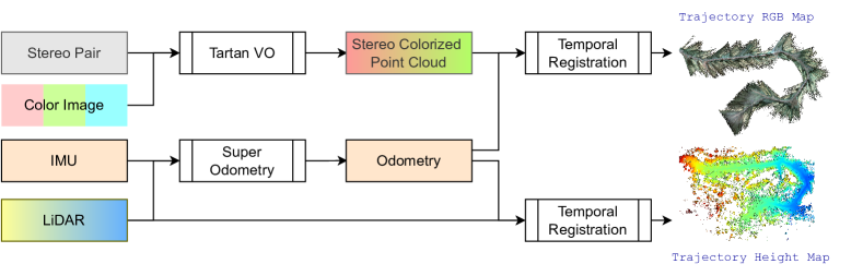
Figure 3: Block diagram of the data generation protocol via future-fusion. The odometry estimation provided by the Super Odometry [36] framework is employed to register the colorized stereo point cloud [37] and LiDAR scans to generate the trajectory RGB and height maps. These dense maps containing billions of points are then utilized to generate dense labels corresponding to the sparse local BEV maps for self-supervision. See Section III-A for details.

III Our Approach

III-A Data Generation by Future-Fusion

Future-fusion pipeline: As described in Section I, the limited sensing range of the offroad ATVs [4] leads to the sparse and noisy measurement starting from as close as about $6m$ from the ego-vehicle. Thus, to denoise and complete the map up to the serviceable range of $30m$ ahead, first, we generate dense and reasonably accurate BEV RGB and heightmaps for $12m\times 30m$ which we can employ to train our completion model.

Figure 4: Comparison of different pixel attibution strategies for BEV map generation – unweighted average (Avg); inverse-distance weighted average (IDW-Avg); closest point attribution (Closest). The distinctive perceptual quality for the later strategy is evident. Best viewed in digital format.

Figure 3 depicts the pipeline for generating the complete trajectory map. The data generation protocol takes stereo pairs and monocular RGB image, LiDAR scans, and a IMU measurement as input. The stereo matching model responsible for generating the stereo colorized point cloud is taken from TartanVO [37]. Moreover, we employ Super Odometry [36] as our in-house odometry estimation method which relies on IMU and LiDAR measurements. With the estimated odometry, the temporal registration blocks (Figure 3) independently register the local colorized stereo point cloud and LiDAR scans into the global frame to generate the complete trajectory RGB and height maps.

In the next step, we generate per-frame input and label RGB and height maps. This is essentially running the same pipeline as above with some additional steps. One is the additional transformation of the complete map from above to the local coordinates for each frame as well. The accumulation from previous history contains the input map whereas the complete map represents the future-fusion labels for self-supervision. Also, we set the local coordinate frame on the ground right under the body frame of our ATV. The yaw of the local frame matches the bearing of the vehicle and the roll and pitch are set to zero. This is to make the local height measurements indicative of the potential slope of the upcoming terrain.

Pixel attribution strategies: The conventional way to generate per-point BEV attribute is the maximum likelihood (ML) estimate which is the unweighted average $\sum_{i=1}^{n}\mathbf{x}_{i}/n$ of the candidate points if the noise distribution is assumed to be a Gaussian. However, we find this estimate produces a quite blurry version of the dense maps (Figure 4). A better choice is the weighted average $\sum_{i=1}^{n}w_{i}\mathbf{x}_{i}$ where $\sum_{i=1}^{n}w_{i}=1$ and the weights are the inverse of the ego-distance $w_{i}=1/\sqrt{x_{i}^{2}+y_{i}^{2}+z_{i}^{2}}$ which is less susceptible to the outliers. However, given that we employ stereo point clouds [37] for this task, some of the candidates with higher ego-distance may evolve as a consequence similar to the singularity of the triangulation method [38]. Thus, we opt for the candidate with the closest ego distance, i.e. $\mathbf{x}=\underset{\mathbf{x}_{i}}{\operatorname*{arg\,min}}\{d(\mathbf{x}_{i})\}$ where $d(\mathbf{x}_{i})=\sqrt{x_{i}^{2}+y_{i}^{2}+z_{i}^{2}}$. Note that this ego-distance refers to the distance from the recording sensor before registration. We empirically find this choice of closest candidate produces perceptually much higher quality samples than other schemes mentioned above for tiny or narrow objects like gravels and mud slick as shown in Figure 4. However, since LiDAR scans are not affected by such noise within our target limit of $30m$, we employ the inverse distance weighted averaging from above for the LiDAR height maps.

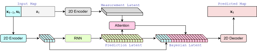
Figure 5: Schematics of the deep Bayesian fusion mechanism. The input is split into two disjoint sub-regions: (1) smaller, proximal, and reliable one resembling the combined previous state $\mathbf{x}_{t-1}$ and control action $\mathbf{u}_{t}$, and (2) distal, sparse and noisy one equivalent to the measurement $\mathbf{z}_{t}$. (Prediction step) The distal latent is predicted by unrolling the proximal latent via RNN. (Measurement update) The predicted roll out is modulated by the noisy distal latent via cross-attention mechanism. Finally, the fused latent is decoded into the complete local BEV map representing the current state $\mathbf{x}_{t}$.

III-B Deep Bayesian Future Fusion

Motivation: A standard deep network trained with a combination of generative losses performs well when the input does not contain significantly varying degrees of noise and / or sparsity. However, we empirically find such a setup falls short for our case where such noise is present in the input as a nonlinear function of distance. Thus, to make the model explicitly aware of this noise structure, we inscribe a mechanism similar to Bayes filtering [5] in this paper.

Preliminary background: The governing equations underlying the problem of state estimation are given by [5]:

$$\mathbf{x}_{t}=g(\mathbf{x}_{t-1},\mathbf{u}_{t})+\omega_{t}$$

$$\mathbf{z}_{t}=h(\mathbf{x}_{t})+\nu_{t}$$

Here, $\mathbf{x}_{t},\;\mathbf{z}_{t},\;\mathbf{u}_{t}$ denote the state representation, measurement, and control actions at time $t$. Moreover, $\omega_{t}$ and $\nu_{t}$ are the additive process and measurement noise terms, respectively. With the Markovian assumption, the posterior is, therefore, can be expressed as follows:

$$p(\mathbf{x}_{t}|\mathbf{x}_{t-1},\mathbf{u}_{t},\mathbf{z}_{t})=\eta\;p(\mathbf{z}_{t}|\mathbf{x}_{t})\;p(\mathbf{x}_{t}|\mathbf{x}_{t-1},\mathbf{u}_{t})$$

In this equation, the estimation task is factorized into the prediction step (second term) followed by the measurement update (first term). In general, the approximation models act like a MAP estimator [39] for the individual factors where we can express them as follows:

$$\phi(\mathbf{x}_{t}|\mathbf{x}_{t-1},\mathbf{u}_{t},\mathbf{z}_{t})=\chi\left(\theta(\mathbf{z}_{t}|\mathbf{x}_{t}),\;\psi(\mathbf{x}_{t}|\mathbf{x}_{t-1},\mathbf{u}_{t})\right)$$ (1)

Here, $\theta,\;\psi$ represent the approximators (e.g. deep learning models) factorizing the underlying joint distribution of $\phi$, and $\chi$ is the composition operator used to combine the factors, i.e. prediction and noisy measurement.

Deep Bayesian fusion: We start with a preliminary observation that the input BEV map of our servicable range ($12m\times 30m$) is somewhat accurate in the first (or left) $12m\times 6m$ regions. Based on that, we model the factorization in Equation 1 below. Note that we depict the formulation via the standard 2D encoder-decoder architecture here. However, our architecture-agnostic formulation is equally applicable to any other network structure.

$\bullet$ Prediction update, $\psi(\mathbf{x}_{t}|\mathbf{x}_{t-1},\mathbf{u}_{t})$: The initial sub-region of $12m\times 6m$ can be thought of as a composition of both the sufficient information about the previous state $\mathbf{x}_{t-1}$ and the control action for the current state $\mathbf{u}_{t}$. For our BEV completion task, $\mathbf{u}_{t}$ indicates the direction of the planar motion of the ego-vehicle that is implicitly embeeded in this sub-region. For instance, in Figure 6 (second column), $\mathbf{u}_{t}$ guides the network about the curvature of the continuing trail for the upcoming map $\mathbf{x}_{t}$.

We realize $\psi(\mathbf{x}_{t}|\mathbf{x}_{t-1},\mathbf{u}_{t})$ via the 2D CNN encoder and a column-wise RNN encoder-decoder operating on the latent space of the former (Figure 5). First, we pass this left sub-region of RGB and height map representing our $\mathbf{x}_{t-1}$ and $\mathbf{u}_{t}$ to the 2D CNN encoder for a corresponding latent feature map. Note that by design, our local BEV map indicates a somewhat left $\rightarrow$ right motion. A natural way to learn this motion parameters and predict the future states is to employ the recurrent roll out on the latent encoding of the combined $\mathbf{x}_{t-1}$ and $\mathbf{u}_{t}$ extracted before. Therefore, our RNN encoder-decoder performs horizontal (left $\rightarrow$ right) unrolling via rolling out the latent columns one at a time. The RNN encoder is first initialized by the latent columns corresponding to the initial $12m\times 6m$ sub-region. Next, the RNN decoder unrolls the latent columns for the remaining $12m\times 24m$ right sub-region. Despite the sequential nature of the recurrent roll out, it incurs negligible computational overhead due to the significantly lower dimensionality of our downsampled latents (Figure 5).

$\bullet$ Measurement update, $\chi\left(\theta(\mathbf{z}_{t}|\mathbf{x}_{t}),\;\ldots\right)$ : As already explained above, the left $12m\times 6m$ of our $12m\times 30m$ range indicates the previous state $\mathbf{x}_{t-1}$ and control action $\mathbf{u}_{t}$. Thus, the right $12m\times 24m$ represents the sparse measurement $\mathbf{z}_{t}$ with varying degree of noise. The measurement update consists of two steps. First, we realize $\theta(\mathbf{z}_{t}|\mathbf{x}_{t})$ by encoding the $12m\times 24m$ input $\mathbf{z}_{t}$ with a 2D CNN encoder similar to the prediction update. Next, the measurement update $\chi$ is implemented by modulating the unrolled prediction from the prediction step with this measurement latent via scaled dot product attention [40] as follows:

$$\chi(\theta,\psi)=\texttt{softmax}\left(\frac{\psi\theta^{T}}{\sqrt{d_{\theta}}}\right)\theta$$

Here, $\chi,\;\theta,\;\psi$ denotes the output of the corresponding factors from Equation 1, and $d_{\theta}$ is the embedding dimension of $\theta$. Finally, we employ a 2D CNN decoder to generate the dense completion of RGB and heightmap from the deep Bayesian latents $\chi(\theta,\;\psi)$ from above.

Remarks on transformer-based fusion: Contrary to the sequential unrolling mechanism provided by any recurrent structure, transformers [17, 41] predict the temporal dependency in a one-shot manner, and seem to outperform the RNN variants in recent times. However, we empirically found the SOTA encoder-decoder structure based on the transformer [41, 42] produces blurry predictions in the distal regions similar to its vanilla CNN counterpart (e.g. UNet). We hypothesize the reason for such poor quality prediction to be multi-fold. The lower resolution ($1/4$ of input) of the prediction could be a potential reason. Another reason could be the lack of explicit hint about the more noisy nature of right side of the input that we provide by two-step encoding (i.e. prediction and measurement). Overall, our bayesian fusion is also equally applicable for transformers. However, primarily due to their lower-resolution prediction and reasonable performance of the 2D CNN, in this paper, we proceed with the 2D CNN backbones for further analysis. Deciphering the performance of the SOTA transformers for the map completion task is out of scope for this paper.

III-C Loss functions

Apart from the standard reconstruction loss $\mathcal{L}_{rec}$, following the recent advances in generative modeling, in particular, unseen view synthesis [43], we employ adversarial $\mathcal{L}_{adv}$ and perceptual losses $\mathcal{L}_{perp}$ [6, 44] as the additional loss functions for high-level domain alignment. In addition, UNet is chosen as the discriminator for detailed discriminative feedback while training [45]. Overall, the complete loss is given by

$$\mathcal{L}=\lambda_{rec}\mathcal{L}_{rec}+\lambda_{adv}\mathcal{L}_{adv}+\lambda_{perp}\mathcal{L}_{perp}$$ (2)

where $\lambda_{rec}$, $\lambda_{adv}$, and $\lambda_{perp}$ are the interaction hyperparameters chosen empirically.

Figure 6: Sample prediction results (Bayes-UNet/e2) alongside the input and future-fusion labels for both RGB (top) and height (bottom). In some cases (columns 3 and 5), the adversarial or highly variable illumination present in the labels are mitigated in our prediction. We hypothesize such self-supervised correction to be the reason why the prediction sometimes work better on average than the labels on downstream tasks (Table II, III). Best viewed in digital format.

IV Experiments

TABLE I: Comparison of Map Completion Models

Method RGB Height MAE ($\downarrow$) FID ($\downarrow$) SSIM ($\uparrow$) MAE ($\downarrow$) FID ($\downarrow$) SSIM ($\uparrow$) Baseline (Input) 0.1430 9.1001 0.3551 0.8987 9.4244 0.5540 UNet 0.1114 2.5217 0.3847 0.5943 1.9394 0.7029 UNet/e2 0.1106 1.5233 0.3721 0.3799 1.8139 0.7355 Bayes-UNet/e2 0.1082 1.4990 0.3910 0.4039 1.2323 0.7502 Lower is better ($\downarrow$);   Higher is better ($\uparrow$)

In this section, first we describe the statistics of the generated dataset. Next, we compare the deep Bayesian fusion mechanism against the vanilla model, in terms of the direct photometric loss and other metrics used for generative modeling [46, 44, 43]. Next, we validate the map completion results further through the performance on the additional downstream task.

IV-A Datasets

The RGB and heightmap input/label pairs are generated for 28 trajectories (or runs) from the TartanDrive-2.0 [47] dataset. The RGB and stereo pairs are from Multisense S21, and the LiDAR scans contain the points from two Velodyne VLP-32 and a Livox Mid-70 sensors. We hold out $4/28$ trajectories for testing and the rest for training. In total, there are $65134$ and $10307$ input/label BEV pairs of range $12m\times 30m$ in our train/test splits, respectively.

IV-B Architecture

The recent trend of combining the diffusion mechanism with transformers [14, 15, 16] demonstrates promising results for image generation. However, the runtime of the diffusion-based models are far from being real-time for the autonomy stack in the off-road ATVs. Considering that, we utilize the efficient convolutional backbone, UNet [48] with the recent advances in GAN-based loss formulations [6, 44] in this paper.

IV-C Photometric and Generative Evaluation

Table I shows the comparative results for generative modeling. The raw input is our baseline that also serves as the lower bound of performance. For UNet, we stack the RGB and height channels altogether as input, which acts like an early fusion mechanism. For UNet/e2, we split the UNet encoder into half and process RGB and height independently, and merge in the decoding step. This formation resembles a late fusion mechanism. Since UNet/e2 outperforms UNet, we implement our Bayesian fusion mechanism on top of UNet/e2, which we call Bayes-UNet/e2. Note that the roll out here is implemented in the $H/(sd)\times W/(sd)$ where $H\times W$ is the shape of BEV maps, $s(16)$ is the final stride of the model, $d(3)$ is an additional downsampling factor. Thus, the Bayesian mechanism does not incur significant additional cost into the standard model. The Bayesian variant outperforms its vanilla counterparts in most cases (Table I).

IV-D Evaluation on the Downstream Task

We further evaluate on the downstream task of predicting the vehicle dynamics which refers to the prediction of future states $\{s_{i}\}_{1}^{T}$ given the initial state $s_{0}$, the sequence of actions $\mathcal{A}=\{a_{i}\}_{1}^{T}$, and a set of initial multimodal measurements $\mathcal{Z}=z_{0}$. We employ the model from PIAug [8] without the physics-informed loss.

Table II and III list the MAE $\pm$ std over $\{10,20,30\}$seconds horizons at $10Hz$, for both training and evaluation with raw input (Input), future-fusion label (Label), and our Bayes-UNet/e2 predictions (Prediction). In this regard, Input and Label serve as upper and lower bound of errors, respectively. Table II contains the error statistics over all the measurements in a horizon, whereas Table III is for the final timestamp – an indicator of how much the predicted dynamics deviates at the extreme.

For the $10s$ horizon, all the three data types provide comparable performance. However, as the horizon expands, both Label and Prediction excel Input by a significant margin. Overall, Label and Prediction exhibit quite similar performance with Prediction exceeding Label in some of the cases. This seemingly counterintuitive behavior is due to the fact that our map completion model sometimes even marginalizes the adversaries present in Label, such as low contrast and high illumination (Figure 6). This also manifests the goodness of our dense map completion.

TABLE II: Mean Absolute Error (MAE) $\pm$ Std Over All Time Stamps for Vehicle Dynamics Prediction

Horizon Data $\Delta p\;(m)$ $\Delta v\;(m/s)$ $\Delta\psi\;(rad)$ $\Delta\delta\;(rad)$ Mean$\pm$Std % Mean$\pm$Std % Mean$\pm$Std % Mean$\pm$Std % 10s Input 0.220 $\pm$ 0.162 100% 0.219 $\pm$ 0.199 100% 0.023 $\pm$ 0.021 100% 0.030 $\pm$ 0.031 100% Label 0.222 $\pm$ 0.168 100.9% 0.213 $\pm$ 0.210 97.3% 0.022 $\pm$ 0.020 95.7% 0.031 $\pm$ 0.032 103.3% Prediction 0.225 $\pm$ 0.169 102.3% 0.213 $\pm$ 0.210 97.3% 0.022 $\pm$ 0.020 95.7% 0.031 $\pm$ 0.032 103.3% 20s Input 0.851 $\pm$ 0.594 100% 0.432 $\pm$ 0.349 100% 0.071 $\pm$ 0.079 100% 0.046 $\pm$ 0.061 100% Label 0.766 $\pm$ 0.559 90.01% 0.391 $\pm$ 0.363 90.05% 0.063 $\pm$ 0.054 88.73% 0.045 $\pm$ 0.054 97.83% Prediction 0.762 $\pm$ 0.560 89.53% 0.388 $\pm$ 0.362 89.81% 0.063 $\pm$ 0.054 88.73% 0.045 $\pm$ 0.054 97.83% 30s Input 2.628 $\pm$ 1.422 100% 0.650 $\pm$ 0.502 100% 0.142 $\pm$ 0.111 100% 0.058 $\pm$ 0.049 100% Label 2.025 $\pm$ 1.312 77.05% 0.653 $\pm$ 0.451 100.46% 0.119 $\pm$ 0.074 83.8% 0.042 $\pm$ 0.041 72.41% Prediction 2.092 $\pm$ 1.314 79.53% 0.664 $\pm$ 0.447 102.15% 0.119 $\pm$ 0.074 83.8% 0.042 $\pm$ 0.042 72.41% $p\equiv$ Distance; $\psi\equiv$ Yaw; $v\equiv$ Velocity; $\delta\equiv$ Steering;            % errors are expressed relative to the Input row which is always 100%

TABLE III: Mean Absolute Error (MAE) $\pm$ Std Over the Final Time Stamp for Vehicle Dynamics Prediction

Horizon Data $\Delta p\;(m)$ $\Delta v\;(m/s)$ $\Delta\psi\;(rad)$ $\Delta\delta\;(rad)$ Mean$\pm$Std % Mean$\pm$Std % Mean$\pm$Std % Mean$\pm$Std % 10s Input 0.552 $\pm$ 0.432 100% 0.371 $\pm$ 0.362 100% 0.050 $\pm$ 0.049 100% 0.040 $\pm$ 0.055 100% Label 0.568 $\pm$ 0.450 102.9% 0.389 $\pm$ 0.393 104.9% 0.046 $\pm$ 0.046 92% 0.043 $\pm$ 0.057 107.5% Prediction 0.572 $\pm$ 0.450 103.62% 0.389 $\pm$ 0.393 104.9% 0.047 $\pm$ 0.046 94.0% 0.043 $\pm$ 0.057 107.5% 20s Input 2.424 $\pm$ 1.820 100% 0.784 $\pm$ 0.664 100% 0.162 $\pm$ 0.221 100% 0.064 $\pm$ 0.093 100% Label 2.137 $\pm$ 1.599 88.2% 0.721 $\pm$ 0.697 91.9% 0.149 $\pm$ 0.161 91.98% 0.058 $\pm$ 0.084 90.63% Prediction 2.131 $\pm$ 1.604 88.0% 0.714 $\pm$ 0.698 90.9% 0.149 $\pm$ 0.160 91.98% 0.058 $\pm$ 0.084 90.63% 30s Input 6.912 $\pm$ 4.586 100% 1.118 $\pm$ 0.999 100% 0.276 $\pm$ 0.261 100% 0.064$\pm$ 0.066 100% Label 4.975 $\pm$ 3.242 71.98% 1.091 $\pm$ 0.840 97.5% 0.188 $\pm$ 0.146 68.12% 0.041 $\pm$ 0.042 64.06% Prediction 5.146 $\pm$ 3.211 74.44% 1.122 $\pm$ 0.835 100.44% 0.190 $\pm$ 0.148 68.84% 0.041 $\pm$ 0.042 64.06% $p\equiv$ Distance; $\psi\equiv$ Yaw; $v\equiv$ Velocity; $\delta\equiv$ Steering;            % errors are expressed relative to the Input row which is always 100%

V Conclusion and Future Work

In this paper, we propose a self-supervised, scalable map completion framework for off-road navigation fusing the future information from the complete trajectory. Unlike existing literature attempting to solve the downstream tasks somewhat directly, we aim to generate a dense and denoised map at a resolution ($2$cm) significantly larger than the state-of-the-art (i.e. $20$cm). To effectively deal with the variable noise and sparsity, we couple the Bayesian mechanism [5] with SOTA generative loss formulations on top of the efficient convolutional backbone. We demonstrate the efficacy of our framework from both a direct generative modeling perspective and through the lens of a downstream task.

With the advent of faster computes, we plan to increase the mapping range with more data and employ our dense map predictions to assist in diverse downstream tasks. Finally, we hope our domain-agnostic framework will encourage the robotics community in general to pursue similar self-supervised dense mapping protocol for large-scale pretraining in the foreseeable future.

References

- [1] J. Frey, S. Khattak, M. Patel, D. Atha, J. Nubert, C. Padgett, M. Hutter, and P. Spieler, “Roadrunner – learning traversability estimation for autonomous off-road driving,” 2024.
- [2] X. Meng, N. Hatch, A. Lambert, A. Li, N. Wagener, M. Schmittle, J. Lee, W. Yuan, Z. Chen, S. Deng, et al., “Terrainnet: Visual modeling of complex terrain for high-speed, off-road navigation,” 2023.
- [3] A. Geiger, P. Lenz, C. Stiller, and R. Urtasun, “Vision meets robotics: The kitti dataset,” IJRR, 2013.
- [4] S. Triest, M. Sivaprakasam, S. J. Wang, W. Wang, A. M. Johnson, and S. Scherer, “Tartandrive: A large-scale dataset for learning off-road dynamics models,” in ICRA, 2022.
- [5] S. Thrun, W. Burgard, and D. Fox, Probabilistic robotics., ser. Intelligent robotics and autonomous agents. MIT Press, 2005.
- [6] T. Karras, S. Laine, and T. Aila, “A style-based generator architecture for generative adversarial networks,” in CVPR, 2019.
- [7] T. Karras, M. Aittala, J. Hellsten, S. Laine, J. Lehtinen, and T. Aila, “Training generative adversarial networks with limited data,” in NeurIPS, 2020.
- [8] P. Maheshwari, W. Wang, S. Triest, M. Sivaprakasam, S. Aich, J. G. R. I. au2, J. M. Gregory, and S. Scherer, “Piaug – physics informed augmentation for learning vehicle dynamics for off-road navigation,” 2023.
- [9] J. Yu, Z. Lin, J. Yang, X. Shen, X. Lu, and T. Huang, “Free-form image inpainting with gated convolution,” in ICCV, 2019.
- [10] G. Liu, F. A. Reda, K. J. Shih, T.-C. Wang, A. Tao, and B. Catanzaro, “Image inpainting for irregular holes using partial convolutions,” in ECCV, 2018.
- [11] J. Uhrig, N. Schneider, L. Schneider, U. Franke, T. Brox, and A. Geiger, “Sparsity invariant cnns,” CoRR, vol. abs/1708.06500, 2017.
- [12] Y. Jia, “Learning semantic image representations at a large scale,” Ph.D. dissertation, University of California, Berkeley, USA, 2014.
- [13] Z. Yi, Q. Tang, S. Azizi, D. Jang, and Z. Xu, “Contextual residual aggregation for ultra high-resolution image inpainting,” in CVPR, 2020.
- [14] J. Song, C. Meng, and S. Ermon, “Denoising diffusion implicit models,” in ICLR, 2021.
- [15] J. Ho, A. Jain, and P. Abbeel, “Denoising diffusion probabilistic models,” in NeurIPS, H. Larochelle, M. Ranzato, R. Hadsell, M. Balcan, and H. Lin, Eds., 2020.
- [16] W. Peebles and S. Xie, “Scalable diffusion models with transformers,” in ICCV, 2023.
- [17] A. Dosovitskiy, L. Beyer, A. Kolesnikov, D. Weissenborn, X. Zhai, T. Unterthiner, M. Dehghani, M. Minderer, G. Heigold, S. Gelly, J. Uszkoreit, and N. Houlsby, “An image is worth 16x16 words: Transformers for image recognition at scale,” in ICLR, 2021.
- [18] B. Mersch, X. Chen, J. Behley, and C. Stachniss, “Self-supervised point cloud prediction using 3d spatio-temporal convolutional networks,” in CoRL, 2021.
- [19] X. Weng, J. Wang, S. Levine, K. Kitani, and N. Rhinehart, “Inverting the forecasting pipeline with spf2: Sequential pointcloud forecasting for sequential pose forecasting,” in CoRL, 2020.
- [20] X. Weng, J. Nan, K.-H. Lee, R. McAllister, A. Gaidon, N. Rhinehart, and K. M. Kitani, “S2net: Stochastic sequential pointcloud forecasting,” in ECCV, 2022.
- [21] T. Khurana, P. Hu, D. Held, and D. Ramanan, “Point cloud forecasting as a proxy for 4d occupancy forecasting,” in CVPR, 2023.
- [22] “KITTI Depth Completion Evaluation,” https://www.cvlibs.net/datasets/kitti/eval˙depth.php?benchmark=depth˙completion.
- [23] L. Liu, X. Song, J. Sun, X. Lyu, L. Li, Y. Liu, and L. Zhang, “Mff-net: Towards efficient monocular depth completion with multi-modal feature fusion,” IEEE RAL, 2023.
- [24] W. Zhou, X. Yan, Y. Liao, Y. Lin, J. Huang, G. Zhao, S. Cui, and Z. Li, “Bev@dc: Bird’s-eye view assisted training for depth completion,” in CVPR, 2023.
- [25] Z. Yan, K. Wang, X. Li, Z. Zhang, J. Li, and J. Yang, “Rignet: Repetitive image guided network for depth completion,” in ECCV, 2022.
- [26] Y. Lin, T. Cheng, Q. Zhong, W. Zhou, and H. Yang, “Dynamic spatial propagation network for depth completion,” AAAI, 2022.
- [27] Y. Zhang, X. Guo, M. Poggi, Z. Zhu, G. Huang, and S. Mattoccia, “Completionformer: Depth completion with convolutions and vision transformers,” in CVPR, 2023.
- [28] T. Van Dijk and G. De Croon, “How do neural networks see depth in single images?” in ICCV, 2019.
- [29] J. Hu, Y. Zhang, and T. Okatani, “Visualization of convolutional neural networks for monocular depth estimation,” in ICCV, 2019.
- [30] S. Aich, J. M. Uwabeza Vianney, M. Amirul Islam, and M. K. Bingbing Liu, “Bidirectional attention network for monocular depth estimation,” in ICRA, 2021.
- [31] A. Shaban, X. Meng, J. Lee, B. Boots, and D. Fox, “Semantic terrain classification for off-road autonomous driving,” in CoRL, 2022.
- [32] S. Triest, D. D. Fan, S. Scherer, and A.-A. Agha-Mohammadi, “Unrealnet: Learning uncertainty-aware navigation features from high-fidelity scans of real environments,” in ICRA, 2024.
- [33] E. Chen, C. Ho, M. Maulimov, C. Wang, and S. Scherer, “Learning-on-the-drive: Self-supervised adaptation of visual offroad traversability models,” 2023.
- [34] D. D. Fan, K. Otsu, Y. Kubo, A. Dixit, J. Burdick, and A.-A. Agha-Mohammadi, “Step: Stochastic traversability evaluation and planning for risk-aware off-road navigation,” in RSS, 2021.
- [35] T. Jebara, Machine Learning: Discriminative and Generative (Kluwer International Series in Engineering and Computer Science). USA: Kluwer Academic Publishers, 2003.
- [36] S. Zhao, H. Zhang, P. Wang, L. Nogueira, and S. Scherer, “Super odometry: Imu-centric lidar-visual-inertial estimator for challenging environments,” in IROS, 2021.
- [37] W. Wang, Y. Hu, and S. Scherer, “Tartanvo: A generalizable learning-based vo,” in CoRL, 2021.
- [38] R. Hartley and A. Zisserman, Multiple View Geometry in Computer Vision, 2nd ed. Cambridge University Press, 2003.
- [39] C. M. Bishop, Pattern Recognition and Machine Learning (Information Science and Statistics), 1st ed. Springer, 2007.
- [40] A. Vaswani, N. Shazeer, N. Parmar, J. Uszkoreit, L. Jones, A. N. Gomez, L. u. Kaiser, and I. Polosukhin, “Attention is all you need,” in NeurIPS, 2017.
- [41] E. Xie, W. Wang, Z. Yu, A. Anandkumar, J. M. Alvarez, and P. Luo, “Segformer: Simple and efficient design for semantic segmentation with transformers,” in NeurIPS, 2021.
- [42] T. Guan, D. Kothandaraman, R. Chandra, A. J. Sathyamoorthy, K. Weerakoon, and D. Manocha, “Ga-nav: Efficient terrain segmentation for robot navigation in unstructured outdoor environments,” IEEE RAL, vol. 7, no. 3, 2022.
- [43] Y. Ren, X. Fan, G. Li, S. Liu, and T. H. Li, “Neural texture extraction and distribution for controllable person image synthesis,” in CVPR, 2022.
- [44] J. Johnson, A. Alahi, and L. Fei-Fei, “Perceptual losses for real-time style transfer and super-resolution,” in ECCV, 2016.
- [45] E. Schönfeld, B. Schiele, and A. Khoreva, “A u-net based discriminator for generative adversarial networks,” in CVPR, 2020.
- [46] M. Heusel, H. Ramsauer, T. Unterthiner, B. Nessler, and S. Hochreiter, “Gans trained by a two time-scale update rule converge to a local nash equilibrium,” in NeurIPS, 2017.
- [47] M. Sivaprakasam, P. Maheshwari, M. G. Castro, S. Triest, M. Nye, S. Willits, A. Saba, W. Wang, and S. Scherer, “Tartandrive 2.0: More modalities and better infrastructure to further self-supervised learning research in off-road driving tasks,” in ICRA, 2024.
- [48] O. Ronneberger, P. Fischer, and T. Brox, “U-net: Convolutional networks for biomedical image segmentation,” in MICCAI, 2015.
- [49] “DEVCOM Army Research Laboratory,” https://www.arl.army.mil.