Flexible control function approach under different types of dependent censoring

Abstract: In this paper, we consider the problem of estimating the causal effect of an endogenous variable $Z$ on a survival time $T$ that can be subject to different types of dependent censoring. Firstly, we extend the current literature by simultaneously allowing for both independent ($A$) and dependent ($C$) censoring. Moreover, we have different parametric transformations for $T$ and $C$ that result in a more additive structure with approximately normal and homoscedastic error terms. The model is shown to be identified and a two-step estimation method is specified. It is shown that this estimator results in consistent and asymptotically normal estimates. Secondly, a goodness-of-fit test is developed to check the model’s validity. To estimate the distribution of the statistic, a parametric bootstrap approach is used. Lastly, we show how the model naturally extends to a competing risks setting. Simulations are used to evaluate the finite-sample performance of the proposed methods and approaches. Moreover, we investigate two data applications regarding the effect of job training programs on unemployment duration and the effect of periodic screenings on breast cancer mortality rates.

Acknowledgments: The data that support the findings of this study are available from the Cancer Data Access System. Restrictions apply to the availability of these data, which were used under license for this study. Data are available at https://cdas.cancer.gov/ with the permission of the Cancer Data Access System.

Funding: I. Van Keilegom gratefully acknowledges funding from the FWO and F.R.S.-FNRS under the Excellence of Science (EOS) programme, project ASTeRISK (grant No. 40007517). G. Crommen is funded by a PhD fellowship from the Research Foundation - Flanders (grant number 11PKA24N).

1 Introduction

When trying to estimate the causal effect of a treatment variable $Z$ on a right-censored survival time $T$, unmeasured confounding can be an important source of bias. To fix ideas, let $T$ depend on a vector of observed covariates $X$, an observed confounded variable $Z$ and some error term $u_{T}$, which represents unobserved heterogeneity. Since we are most interested in the causal effect of $Z$ on $T$, there is a confounding issue when $Z$ and $u_{T}$ are dependent on each other. Note that this dependence implies that the causal effect of $Z$ on $T$ cannot be identified from the conditional distribution of $T$ on $(X,Z)$. Things are complicated even further by having a right-censoring time $C$, for which we have a similar model as $T$ but with unobserved error term $u_{C}$. This means that only the minimum of $T$ and $C$ is observed through the follow-up time $Y=\min\{T,C\}$ and the censoring indicator $\Delta=\mathbbm{1}(Y=C)$. Note that, contrary to what is commonly done in the survival analysis literature, we do not assume that $T$ and $C$ are independent, even after conditioning on $(X,Z)$. This possible dependence creates an additional statistical issue since the distribution of $T$ cannot be recovered from that of $(Y,\Delta)$ without making further assumptions on the joint and/or marginal distribution of $T$ and $C$. In this work, we build further on the model by Crommen et al., (2024) and extend it in many meaningful ways. In their paper, they (i) propose a control function approach to deal with the unmeasured confounding and (ii) place a bivariate normality assumption on $(u_{T},u_{C})$ to deal with the dependent censoring. Our contributions are the following. Firstly, the bivariate normality assumption placed on the error terms is made more plausible by having different power transformations for both $T$ and $C$. This is because a power transformation to the response of a regression model usually results in a more additive structure with approximately normal and homoscedastic error terms. Moreover, we will also allow for an independent censoring time $A$ (e.g. administrative censoring) such that we observe $Y=\min\{T,C,A\}$, $\Delta=\mathbbm{1}(Y=T)$ and $\xi=\mathbbm{1}(Y=C)$. It is shown that the resulting model remains identifiable, a two-step estimation method is employed and it is shown that the parameter estimates remain consistent and asymptotically normal. Simulation results and a data application regarding the effect of job training programs on unemployment duration are also provided. Secondly, a goodness-of-fit test is developed for the extended model proposed in this paper. Since we only model $T$ and $C$, our test will be based on $K=\min\{T,C\}$ (which is independently censored by $A$). This test is a weighted Cramer–Von Mises type statistic, for which we will estimate the distribution using a parametric bootstrap procedure. Finally, we show how the model naturally extends to a competing risks framework and apply this method to estimate the causal effect of periodic screenings on breast cancer mortality rates. All developed code can be found on our GitHub repository at https://github.com/WillemsIlias/FMCC

1.1 Related literature

A fundamental result in the survival analysis literature comes from Tsiatis, (1975), who proved that the joint distribution of two or more failure times cannot be identified in a nonparametric way by only observing their minimum. This implies that conditions have to be imposed on the joint and/or marginal distribution of the survival and censoring time in order to identify their joint distribution. In the survival analysis literature, it is commonly assumed that the survival time $T$ is (conditionally) independent of the right censoring time $C$. However, this assumption might be violated in some applications (e.g. organ transplant data, unemployment data, …), urging the need to develop models that allow for some form of dependence between $T$ and $C$. In this setting, some models focus on the estimation of the survival curve without including covariates (see Basu and Ghosh, (1978) and Emoto and Matthews, (1990) among others). Currently, the most popular approach is based on the use of copulas. Zheng and Klein, (1995) were the first to introduce this idea, which they called the copula-graphic estimator. It extends the well-known Kaplan and Meier, (1958) estimator to the dependent censoring case. Their method allows for a nonparametric estimator of the marginals of $T$ and $C$ under the assumption of a fully known copula for their joint distribution. Rivest and Wells, (2001) studied the copula-graphic estimator in the special case of Archimedean copulas. The copula-graphic estimator has been extended to include covariates by Braekers and Veraverbeke, (2005), Emura and Chen, (2016) and Sujica and Van Keilegom, (2018) among others. However, all of these extensions still make use of a fully known copula, such that the association parameter needs to be specified. As this is usually not realistic in practice, an alternative approach was proposed by Czado and Van Keilegom, (2023). They show that, in exchange for fully parametric marginals, the association parameter can actually be identified. This can be seen as surprising, since we only observe the minimum of $T$ and $C$. Moreover, Deresa and Van Keilegom, 2020a , Deresa and Van Keilegom, 2020b and Deresa et al., (2022) propose similar methods that also allow for covariates, competing risks and left truncation respectively. Most recently, Deresa and Van Keilegom, (2024) showed that the association parameter is still identifiable when the survival time follows a semiparametric Cox model.

Within the survival analysis literature, instrumental variable methods have already received a lot of attention to estimate causal effects on right censored duration outcomes. However, most of this research has been conducted under the assumption of independent censoring. Frandsen, (2015) and Sant’Anna, (2021) propose nonparametric models when both the instrumental and endogenous variables are binary, relying on the commonly made monotonicity assumption for identification. However, due to this assumption, these models are only able to identify a local treatment effect, i.e. the average treatment effect on the population of compliers. Another nonparametric model imposing a more strict rank invariance assumption has been proposed by Beyhum et al., (2022). By making this assumption, they are able to identify and estimate the average treatment effect on the whole population. A nonparametric model using continuous covariates and discrete or continuous instrumental variables is proposed by Centorrino and Florens, (2021). Semiparametric models have been proposed by Huling et al., (2019), Tchetgen et al., (2015) and Li et al., (2015) among others.

The literature on instrumental variable methods under dependent censoring seems to be sparse. The first relevant work in this context is the paper of Robins and Finkelstein, (2000). They impose that conditionally on the treatment arm and the recorded history of each patient, the cause-specific hazard of censoring no longer depends on the survival time $T$. This implies that all covariates causing a dependence between the survival time and the censoring time are observed. Note that this is very unlikely to happen in practice, as it is difficult to define all covariates causing a dependence between $T$ and $C$. Another model is proposed by Khan and Tamer, (2009). This model aims at constructing point estimates for the survival time, while weakening many assumptions that were previously made in the literature. The model allows for multiple endogenous covariates, dependent censoring and conditionally heteroscedastic error terms. However, a drawback of the model is that their assumptions require the support of the log-transformed censoring time $C$, conditionally on the instrumental variables $\tilde{W}$, to be bounded from below. Moreover, there are some stringent assumptions on the support of the measured covariates and the treatment conditional on the instrument. A third model comes from Blanco et al., (2020), who derive bounds for the treatment effect (in terms of average and quantiles) in a nonparametric way while taking into account dependent censoring, self-selection and non-compliance. The main downside of this approach is that it is only concerned with estimating bounds on the treatment effect, which are often wide and uninformative. Lastly, Crommen et al., (2024) proposed a fully parametric model that allows for dependent censoring and an endogenous treatment variable. Their model uses a control function approach that follows from specifying the reduced form. It is assumed that the natural logarithm of $T$ and $C$ follow a bivariate normal distribution, conditionally on the covariates and the control function. This assumption, combined with an implicit rank invariance assumption, might be too stringent in practice.

1.2 Outline

In Section 2, the model is specified together with some useful distributions and definitions. In section 3 it will be argued that the proposed model is identified. Moreover, the likelihood will be defined and the estimation method explained. We prove consistency and asymptotic normality of the estimator. In Section 4 a goodness-of-fit test is discussed. Section 5 contains a simulation study that assesses the finite sample performance of our methodology and Section 6 uses the approach to study the effect of job training programs on the time until employment. Section 7 extends our model to the case of multiple competing events and has its own simulation study. We provide a data application by studying the effect of periodic screening on breast cancer mortality rates.

2 The model

2.1 Model specification

Let $T$, $C$ and $A$ denote the logarithm of the survival time, dependent censoring time and independent censoring time (e.g. administrative censoring) respectively. Note that only the minimum of $T$, $C$ and $A$ will be observed, that is, we observe the follow-up time $Y=\min(T,C,A)$ and the censoring indicators $\Delta=\mathbbm{1}(Y=T)$ and $\xi=\mathbbm{1}(Y=C)$. The exogenous covariates, influencing both the survival and censoring time, are given by $X=(1,\tilde{X}^{\top})^{\top}$, where $\tilde{X}$ is of dimension $m$. The endogenous variable, which is assumed to be univariate, is denoted by $Z$. More precisely, we propose the following joint regression model:

$$\left\{\begin{array}[]{ll}\Lambda_{\theta_{1}}(T)=X^{\top}\beta_{T}+Z\alpha_{T}+V\lambda_{T}+\epsilon_{T}\\ \Lambda_{\theta_{2}}(C)=X^{\top}\beta_{C}+Z\alpha_{C}+V\lambda_{C}+\epsilon_{C}\end{array}\right.,$$ (1)

where $(\epsilon_{T},\epsilon_{C})$ are unobserved error terms, $\Lambda_{\theta}(\cdot)$ is a power transformation known up to $\theta$, such that $\theta_{1}$ is allowed to be different from $\theta_{2}$, and $V$ an unobserved confounder of $Z$. Since $V$ is not observed, we use an instrumental variable $\tilde{W}$ that is sufficiently dependent on $Z$ (conditionally on $X$) to be able to identify the causal effect of interest $\alpha_{T}$. More precisely, we let $V=g_{\gamma}(Z,W)$, with $W=(X^{\top},\tilde{W})$, for which the control function $g$ is known up to the parameter $\gamma$. Note that this control function follows from the reduced form, which is specified by the analyst. A simple example can be given by

$$V=Z-W^{\top}\gamma,$$ (2)

when $Z$ is continuous and linearly related to $W$, that is,

$$Z=W^{\top}\gamma+\nu\quad\text{with}\quad\operatorname{\mathbb{E}}[\nu\mid W]=0.$$

Another, more involved, example of a control function is

$$V=Z\operatorname{\mathbb{E}}[\nu\mid W^{\top}{\gamma}>\nu]+(1-Z)\operatorname{\mathbb{E}}[\nu\mid W^{\top}{\gamma}<\nu],$$ (3)

when $Z$ is binary and the relation between $Z$ and $W$ is specified as

$$Z=\mathbbm{1}(W^{\top}\gamma>\nu)\quad\text{with}\quad\nu\perp\!\!\!\perp W.$$

We refer to Wooldridge, (2010), Navarro, (2010) and Tchetgen et al., (2015) for a further justification and other examples of the control function approach. Further, it is assumed that:

1. $\begin{pmatrix}\epsilon_{T}\\ \epsilon_{C}\end{pmatrix}\sim\mathcal{N}\left(\begin{pmatrix}0\\ 0\end{pmatrix},\Sigma_{\epsilon}=\begin{pmatrix}\sigma_{T}^{2}&\rho\sigma_{T}\sigma_{C}\\ \rho\sigma_{T}\sigma_{C}&\sigma_{C}^{2}\end{pmatrix}\right),$

   where $\Sigma_{\epsilon}$ is a positive definite matrix (i.e. $\sigma_{T},\sigma_{C}>0$ and $|\rho|<1$).

2. $(\epsilon_{T},\epsilon_{C},A)\perp\!\!\!\perp(W^{\top},Z)$.

3. $(T,C)$ and $A$ are conditionally independent, given $(W^{\top},Z)$.

4. The covariance matrix of $(\tilde{X}^{\top},Z,V)$ has full rank and $\text{Var}(\tilde{W})>0$.

5. The probabilities $P(Y=T|W,Z)$, $P(Y=C|W,Z)$ and $P(Y=A|W,Z)$ are strictly positive.

6. Administrative censoring by $A$ is non-informative for $(T,C)$ given $(W^{\top},Z)$.

7. $\{\Lambda_{\theta}:\theta\in\Theta\}$ is a family of strictly increasing, continuously differentiable transformations, defined on the whole real line and for which it holds that $\lim_{t\rightarrow\pm\infty}{\Lambda_{\theta}(t)}=\pm\infty$ for all $\theta\in\Theta$.

8. For all $\theta_{j}\in\Theta,\mu_{j}\in\mathbb{R},\sigma_{j}>0$, $j=1,2$ it holds that if $\theta_{1}\neq\theta_{2}$, then the limit

   $$\lim_{t\rightarrow\pm\infty}{K_{\theta_{1},\mu_{1},\sigma_{1}}(t)/K_{\theta_{2},\mu_{2},\sigma_{2}}(t)=0\text{ or }\infty},$$

   with

   $$K_{\theta,\mu,\sigma}(t)=\exp\biggl{(}-\frac{1}{2}\biggl{\{}\frac{\Lambda_{\theta}(t)-\mu}{\sigma}\biggl{\}}^{2}\biggl{)}\Lambda_{\theta}^{\prime}(t).$$

Assumption (A1) implies that, conditional on $(X,Z,V)$, both $\Lambda_{\theta_{1}}(T)$ and $\Lambda_{\theta_{2}}(C)$ are normally distributed and allowed to be dependent on each other through a Gaussian copula with association parameter $\rho$. This is a strong assumption to make, but it will later be shown by Theorem 1 that this allows us to actually identify the association parameter $\rho$. This can be seen as surprising, as it means that we can identify the relationship between $\Lambda_{\theta_{1}}(T)$ and $\Lambda_{\theta_{2}}(C)$ while only observing the minimum of $\{T,C,A\}$. In contrast to the model proposed by Crommen et al., (2024), we allow for an independent censoring time $A$ (e.g. administrative censoring). Moreover, Assumption (A1) is placed on the error terms of the transformed survival and censoring time. Therefore, $\Lambda_{\theta}(\cdot)$ should be a transformation that aims to improve normality. It is well known that applying a power transformation to the response of a regression model results in a more additive structure with approximately normal and homoscedastic error terms (Box and Cox,, 1964). The most commonly used example of such a power transformation is the Box-Cox transformation. However, it is clear that this transformation does not satisfy Assumptions (A7) and (A8). A transformation that does satisfy both of these assumptions is the Yeo–Johnson transformation, which can be seen as an extension of the Box-Cox transformation to the whole real line (Yeo and Johnson,, 2000). This transformation can be written as:

$$\Lambda_{\theta}(t)=\left\{\begin{array}[]{ll}\{(t+1)^{\theta}-1\}/\theta&t\geq 0,\theta\neq 0\\ \log(t+1)&t\geq 0,\theta=0\\ -\{(-t+1)^{2-\theta}-1\}/(2-\theta)&t<0,\theta\neq 2\\ -\log(-t+1)&t<0,\theta=2\\ \end{array}\right..$$ (4)

Note that when $\theta=1$, this transformation is the identity transformation on the whole real line. When $1<\theta\leq 2$, the transformation is convex, implying a contraction of the lower part of the support and an extension of the upper part, decreasing skewness to the left. When $0\leq\theta<1$, the transformation is concave and decreases the skewness to the right. Hence, the transformation tries to improve the symmetry of the distribution. As is the case for the Box-Cox transformation, the Yeo-Johnson transformation aims to improve normality, making the bivariate normal error distribution in (A1) more plausible. In Section B of the Supplementary Material, it is verified that this transformation indeed satisfies Assumption (A8).

2.2 Useful definitions and distributions

For the remainder of this paper, it will be useful to have some definitions and distributions at hand with which we can more easily state and prove our results. We observe the random vector $S=(Y,\Delta,\xi,\tilde{X},\tilde{W},Z)$, which takes values in the space $\mathcal{G}=\mathbb{R}\times\{0,1\}\times\{0,1\}\times\mathbb{R}^{m}\times\mathbb{R}\times\mathbb{R}$. Denote the parameter space of $\gamma$ with $\Gamma\subset\mathbb{R}^{m+2}$. The parameter space of $\eta$ is denoted by

$$\mathcal{H}\subset\{\eta:(\underbrace{\beta_{T}^{\top},\alpha_{T},\lambda_{T},\beta_{C}^{\top},\alpha_{C},\lambda_{C}}_{\in\mathbb{R}^{2m+6}},\underbrace{\sigma_{T},\sigma_{C}}_{\in\mathbb{R}^{2}_{>0}},\underbrace{\rho}_{\in(-1,1)},\underbrace{\theta_{1},\theta_{2}}_{\in\Theta\times\Theta})\}.$$

We present some distributions that are used in obtaining the log-likelihood of our model. For ease of notation, we define:

$$\tau_{T}=x^{\top}\beta_{T}+z\alpha_{T}+g_{\gamma}(z,w)\lambda_{T}, b_{T}=\Lambda_{\theta_{1}}(y)-x^{\top}\beta_{T}-z\alpha_{T}-g_{\gamma}(z,w)\lambda_{T},$$

$$\tau_{C}=x^{\top}\beta_{C}+z\alpha_{C}+g_{\gamma}(z,w)\lambda_{C}, b_{C}=\Lambda_{\theta_{2}}(y)-x^{\top}\beta_{C}-z\alpha_{C}-g_{\gamma}(z,w)\lambda_{C}.$$

Since each subject can either experience the event of interest, the dependent censoring event or the administrative censoring event, the likelihood will consist of three parts. The following equations show the contribution of an observation to the likelihood in the cases $T,C$ or $A$ are observed respectively:

$$f_{Y,\Delta,\xi|W,Z}(y,1,0|w,z,\gamma;\eta)$$

$$\quad=\frac{1}{\sigma_{T}}\left[1-\Phi\left(\frac{b_{C}-\rho\frac{\sigma_{C}}{\sigma_{T}}b_{T}}{\sigma_{C}(1-\rho^{2})^{1/2}}\right)\right]\phi\left(\frac{b_{T}}{\sigma_{T}}\right)\Lambda_{\theta_{1}}^{\prime}(y)P(A>y),$$

$$f_{Y,\Delta,\xi|W,Z}(y,0,1|w,z,\gamma;\eta)$$

$$\quad=\frac{1}{\sigma_{C}}\left[1-\Phi\left(\frac{b_{T}-\rho\frac{\sigma_{T}}{\sigma_{C}}b_{C}}{\sigma_{T}(1-\rho^{2})^{1/2}}\right)\right]\phi\left(\frac{b_{C}}{\sigma_{C}}\right)\Lambda_{\theta_{2}}^{\prime}(y)P(A>y),$$

$$f_{Y,\Delta,\xi|W,Z}(y,0,0|w,z,\gamma;\eta)=\bar{\Phi}\left(\frac{b_{T}}{\sigma_{T}},\frac{b_{C}}{\sigma_{C}};\rho\right)f_{A}(y),$$

where $\bar{\Phi}(\cdot,\cdot,\rho)$ is the tail probability of a standard bivariate normal distribution with variance-covariance matrix $\begin{pmatrix}1&\rho\\ \rho&1\end{pmatrix}$. All derivations can be found in Section A of the Supplementary Material. The log-likelihood of our model can now be defined as:

$$l:\mathcal{G}\times\Gamma\times\mathcal{H}\rightarrow\mathbb{R}:(s,\gamma,\eta)\rightarrow l(s,\gamma,\eta)=\log f_{Y,\Delta,\xi|W,Z}(y,\Delta,\xi|w,z,\gamma;\eta),$$

such that the expected log-likelihood is equal to:

$$L(\gamma,\eta)=\operatorname{\mathbb{E}}[l(S,\gamma,\eta)]=\int_{\mathcal{G}}l(s,\gamma,\eta)dG(s),$$ (5)

where $G$ is the distribution function of $S$.

3 Model identification and estimation

3.1 Model identification

Even though we only observe the minimun of $T,C$ and $A$ through the follow-up time $Y$ and censoring indicators $(\Delta,\xi)$, it can be shown that model (1) is identified. With identified, it is meant that two different sets of the parameters $(\gamma,\eta)$ imply two different joint distributions of $S$. Suppose that $(\gamma^{*},\eta^{*})$ are the true values of the parameters. We will assume that

1. $\gamma^{*}$ is identified,

which is satisfied for many commonly used control functions such as (2) and (3). It is important to note that the extra flexibility introduced by allowing different transformations for both $T$ and $C$ substantially complicates the identifiability proof, as it is possible that $T<C$ but $\Lambda_{\theta_{1}}(T)>\Lambda_{\theta_{2}}(C)$. The following theorem is proven in Section C of the Supplementary Material:

Theorem 1.

Under Assumptions (A1) to (A9), suppose that ($T_{1}$,$C_{1}$,$A_{1}$) and ($T_{2}$,$C_{2}$,$A_{2}$) both satisfy model (1) with parameter vectors $(\gamma_{1},\eta_{1})$ and $(\gamma_{2},\eta_{2})$ respectively and define $Y_{j}$, $\Delta_{j}$ and $\xi_{j}$ for $j\in\{1,2\}$ analogous to before. Then if $f_{Y_{1},\Delta_{1},\xi_{1}|W,Z}(\cdot,k_{1},k_{2}|w,z,\gamma_{1};\eta_{1})\equiv f_{Y_{2},\Delta_{2},\xi_{2}|W,Z}(\cdot,k_{1},k_{2}|w,z,\gamma_{2};\eta_{2})$ for each $(k_{1},k_{2})\in\{0,1\}^{2}$ and for almost every $(w,z)$, it follows that:

$$\eta_{1}=\eta_{2}.$$

It should also be noted that (1) is a parametric copula model. Indeed, we impose that parametric transformations of $T$ and $C$ follow a certain normal distribution and model the dependence structure with a Gaussian copula. This puts us in a context that is similar to the one studied in Czado and Van Keilegom, (2023), who study a broader family of models by allowing for different choices for the marginals and copula, but do not include covariates in their analysis (and a fortiori do not need to treat the issue of endogeneity). As is also the case here, identification of such models proves to be the main difficulty.

3.2 Estimation of model parameters

To estimate the model parameters, we use a two-step estimation procedure and refer to the resulting estimator as the two-step estimator. In the first step, $\gamma$ is estimated. Its estimate $\hat{\gamma}$ can then be used in the second step to estimate $\eta$. Note that using $\hat{\gamma}$ instead of the true (unknown) value will increase the variance of the estimator for $\eta$. Assume that the data consist of i.i.d. observations $\{Y_{i},\Delta_{i},\xi_{i},W_{i},Z_{i}\}_{i=1,\dots,n}$. For the first step in the estimation procedure, we make the following assumption:

1. There exist a known function $m:(w,z,\gamma)\in\mathbb{R}^{m+2}\times\mathbb{R}\times\Gamma\rightarrow m(w,z,\gamma)$ that is twice continuously differentiable with respect to $\gamma$ such that

   $$\hat{\gamma}\in\operatorname*{arg\,max}_{\gamma\in\Gamma}{n^{-1}\sum_{i=1}^{n}{m(W_{i},Z_{i},\gamma)}}$$

   is a consistent estimator for the true parameter $\gamma^{*}$.

Theorem 2.1 in Newey and McFadden, (1994) provides sufficient conditions for $\hat{\gamma}$ to be consistent. In the case of control function $\eqref{eq:CF_Z_continuous}$, it can easily be shown that Assumption (A10) follows directly from Assumption (A4) by using ordinary least squares to estimate $\gamma$. When $Z$ is a binary random variable and control function (3) is specified, this assumption follows from Assumption (A4) and a known distributional assumption for $\nu$ (see Aldrich and Nelson, (1991) for more details). With the estimate $\hat{\gamma}$ from the first step, we can continue with estimating $\eta$ in a second step. Based on the definition of the expected log-likelihood in (5), the log-likelihood function that will be maximized as a function of $\eta$ over the parameter space $\mathcal{H}$ is given by:

$$\hat{L}(\hat{\gamma},\eta) =\frac{1}{n}\sum_{i=1}^{n}\log f_{Y,\Delta,\xi|W,Z}(Y_{i},\Delta_{i},\xi_{i}|W_{i},Z_{i},\hat{\gamma};\eta)$$

$$=\frac{1}{n}\sum_{i=1}^{n}{\log\biggl{(}\biggl{\{}\frac{1}{\sigma_{T}}\biggl{[}1-\Phi\biggl{(}\frac{b_{C_{i}}-\rho\frac{\sigma_{C}}{\sigma_{T}}b_{T_{i}}}{\sigma_{C}(1-\rho^{2})^{1/2}}\biggl{)}\biggl{]}\phi\biggl{(}\frac{b_{T_{i}}}{\sigma_{T}}\biggl{)}\Lambda_{\theta_{1}}^{\prime}(Y_{i})\biggl{\}}^{\Delta_{i}}}$$

$$\quad\times\biggl{\{}\frac{1}{\sigma_{C}}\biggl{[}1-\Phi\biggl{(}\frac{b_{T_{i}}-\rho\frac{\sigma_{T}}{\sigma_{C}}b_{C_{i}}}{\sigma_{T}(1-\rho^{2})^{1/2}}\biggl{)}\biggl{]}\phi\biggl{(}\frac{b_{C_{i}}}{\sigma_{C}}\biggl{)}\Lambda_{\theta_{2}}^{\prime}(Y_{i})\biggl{\}}^{\xi_{i}}$$

$$\quad\times\biggl{\{}\bar{\Phi}\biggl{(}\frac{b_{T_{i}}}{\sigma_{T}},\frac{b_{C_{i}}}{\sigma_{C}};\rho\biggl{)}\biggl{\}}^{1-(\Delta_{i}+\xi_{i})}\biggl{)},$$

where

$$b_{T_{i}}=\Lambda_{\theta_{1}}(Y_{i})-X_{i}^{\top}\beta_{T}-Z_{i}\alpha_{T}-g_{\hat{\gamma}}(W_{i},Z_{i})\lambda_{T},$$

and

$$b_{C_{i}}=\Lambda_{\theta_{2}}(Y_{i})-X_{i}^{\top}\beta_{C}-Z_{i}\alpha_{C}-g_{\hat{\gamma}}(W_{i},Z_{i})\lambda_{C}.$$

The estimator of $\eta$ is then equal to

$$\hat{\eta}=(\hat{\beta}_{T}^{\top},\hat{\alpha}_{T},\hat{\lambda}_{T},\hat{\beta}_{C}^{\top},\hat{\alpha}_{C},\hat{\lambda}_{C},\hat{\sigma}_{T},\hat{\sigma}_{C},\hat{\rho},\hat{\theta}_{1},\hat{\theta}_{2})^{\top}=\operatorname*{arg\,max}_{\eta\in\mathcal{H}}\hat{L}(\hat{\gamma},\eta).$$ (6)

3.3 Consistency and asymptotic normality

First of all, some notation that will be useful in this section is defined:

$$h_{l}(S,\gamma^{*},\eta^{*})=\nabla_{\eta}l(S,\gamma^{*},\eta^{*}), H_{\eta}=\operatorname{\mathbb{E}}[\nabla_{\eta}h_{l}(S,\gamma^{*},\eta^{*})],$$

$$h_{m}(W,Z,\gamma^{*})=\nabla_{\gamma}m(W,Z,\gamma^{*}), H_{\gamma}=\operatorname{\mathbb{E}}[\nabla_{\gamma}h_{l}(S,\gamma^{*},\eta^{*})],$$

$$M=\operatorname{\mathbb{E}}[\nabla_{\gamma}h_{m}(W,Z,\gamma^{*})], \Psi=-M^{-1}h_{m}(W,Z,\gamma^{*}),$$

$$\tilde{h}(S,\gamma^{*},\eta^{*})=(h_{m}(W,Z,\gamma^{*})^{\top},h_{l}(S,\gamma^{*},\eta^{*})^{\top})^{\top}, H=\operatorname{\mathbb{E}}[\nabla_{\gamma,\eta}\tilde{h}(S,\gamma^{*},\eta^{*})].$$

Assumption (A10) already states that $\hat{\gamma}$ is a consistent estimator for $\gamma^{*}$. Under some additional assumptions, it can also be proven that $\hat{\eta}$ is a consistent and asymptotically normal estimator of the true parameter $\eta^{*}$. These assumptions are:

1. $\eta^{*}$ belongs to the interior of a compact parameter space $\mathcal{H}$.

2. A function $\mathcal{D}(s)$, integrable with respect to $G$, and a compact neighbourhood $\mathcal{N}_{\gamma}\subset\Gamma$ of $\gamma^{*}$ exist such that $|l(s,\gamma,\eta)|\leq\mathcal{D}(s)$ for all $\gamma\in\mathcal{N}_{\gamma}$ and $\eta\in\mathcal{H}$.

3. $\operatorname{\mathbb{E}}\left[\|\tilde{h}(S,\gamma^{*},\eta^{*})\|^{2}\right]<\infty$ and $\operatorname{\mathbb{E}}\left[\sup_{(\gamma,\eta)\in\mathcal{N}_{\gamma,\eta}}\|\nabla_{\gamma,\eta}\tilde{h}(S,\gamma,\eta)\|\right]<\infty$ where $\mathcal{N}_{\gamma,\eta}$ is a neighbourhood of $(\gamma^{*},\eta^{*})$ in $\Gamma\times\mathcal{H}$.

4. The matrix $H^{\top}H$ is nonsingular.

As usual, $\|\cdot\|$ denotes the Euclidean norm. Assumptions (A11), (A13) and (A14) are a commonly made assumption in maximum likelihood theory. A set of sufficient conditions for (A12) to hold is that $\Gamma$ is compact (which, together with (A11), implies the existence of $\mathcal{N}_{\gamma}$) and that the support of $S$, denoted by $\mathcal{S}$, is bounded (in which case we can define $\mathcal{D}(s)\equiv\max_{\mathcal{S},\Gamma,\mathcal{H}}|l(s,\gamma,\eta)|$). The following two theorems can now be formulated:

Theorem 2.

Assuming (A1) until (A12) and $\hat{\eta}$ as defined in (6), it holds that

$$\hat{\eta}\xrightarrow{p}\eta^{*}.$$

Theorem 3.

Assuming (A1) until (A14) and $\hat{\eta}$ as defined in (6), it holds that

$$\sqrt{n}(\hat{\eta}-\eta^{*})\xrightarrow{d}\mathcal{N}(0,\Sigma_{\eta}),$$

with

$$\Sigma_{\eta}=H_{\eta}^{-1}\operatorname{\mathbb{E}}[\{h_{l}(S,\gamma^{*},\eta^{*})+H_{\gamma}\Psi\}\{h_{l}(S,\gamma^{*},\eta^{*})+H_{\gamma}\Psi\}^{\top}](H_{\eta}^{-1})^{\top}.$$

The proofs of these theorems can be found in Section C of the Supplementary Material.

3.4 Asymptotic variance

Following Theorem 3, a consistent estimator $\hat{\Sigma}_{\eta}$ for the covariance matrix can be defined as:

$$\hat{\Sigma}_{\eta}=\hat{H}_{\eta}^{-1}[n^{-1}\sum_{i=1}^{n}{\{h_{l}(S_{i},\hat{\gamma},\hat{\eta})+\hat{H}_{\gamma}\hat{\Psi}_{i}\}\{h_{l}(S_{i},\hat{\gamma},\hat{\eta})+\hat{H}_{\gamma}\hat{\Psi}_{i}\}^{\top}}](\hat{H}_{\eta}^{-1})^{\top},$$

with

$$\hat{H}_{\eta}=n^{-1}\sum_{i=1}^{n}{\nabla_{\eta}h_{l}(S_{i},\hat{\gamma},\hat{\eta})}, \hat{H}_{\gamma}=n^{-1}\sum_{i=1}^{n}{\nabla_{\gamma}h_{l}(S_{i},\hat{\gamma},\hat{\eta})},$$

$$\hat{M}=n^{-1}\sum_{i=1}^{n}{\nabla_{\gamma}h_{m}(W_{i},Z_{i},\hat{\gamma})}, \hat{\Psi}_{i}=-\hat{M}^{-1}h_{m}(W_{i},Z_{i},\hat{\gamma}).$$

Using this asymptotic variance-covariance matrix estimate, asymptotic confidence intervals for $\eta$ can easily be constructed. To avoid negative values in the confidence intervals of $\sigma_{C}>0$ and $\sigma_{T}>0$, a log-transformation will be used. For similar reasons, a Fisher’s z-transformation will be used to construct confidence intervals for $\rho\in(-1,1)$. The Delta method can be used to obtain the standard errors on the transformed scale and the obtained confidence intervals can than be transformed back to the original scale.

4 Goodness-of-fit test

In the following section, we discuss a goodness-of-fit test for model (1) on a given data set. Recall that the observed times $Y$ correspond to events $(T)$, censoring $(C)$ or administrative censoring $(A)$. However, since we only model $T$ and $C$, we will not construct a goodness-of-fit test for all observed times $Y=\min(T,C,A)$, but rather define $K=\min(T,C)$ and construct a goodness-of-fit test based on $K$, which will be right-censored by $A$. The test will be based on a weighted Cramer–Von Mises type statistic, for which we will estimate the distribution using a parametric bootstrap procedure (see Efron and Tibshirani, (1998) for more details). The test will be such that rejection of the null hypothesis indicates a bad fit, but failing to reject the null hypothesis does not necessarily indicate a good fit. This is because like most statistical tests, there is the possibility of making a type-I error, but additionally, we are only testing on $K$ and not on $T$ and $C$ separately. This means that we cannot directly test the goodness-of-fit of the models for $T$ and $C$ separately, but can only gauge it through testing the goodness-of-fit of the overall model. As a result, the test will be slightly conservative.

To make this more precise, the null hypothesis of the test is

$$H_{0}:P(K\leq k)=F_{K}(k;\gamma^{*},\eta^{*})\quad\forall k\in\mathbb{R},$$

where $F_{K}(k;\gamma^{*},\eta^{*})$ denotes the cumulative distribution function of $K$ that follows from model (1) using the true set of parameters $(\gamma^{*},\eta^{*})$. It follows that

$$F_{K}(k;\gamma,\eta) =\iiint\Phi\left(\frac{\Lambda_{\theta_{1}}(k)-\tau_{T}}{\sigma_{T}}\right)f_{\tilde{X},\tilde{W},Z}(x,w,z)dxdwdz$$

$$\quad+\iiint\Phi\left(\frac{\Lambda_{\theta_{2}}(k)-\tau_{C}}{\sigma_{C}}\right)f_{\tilde{X},\tilde{W},Z}(x,w,z)dxdwdz$$

$$\quad-\iiint\Phi\left(\frac{\Lambda_{\theta_{1}}(k)-\tau_{T}}{\sigma_{T}},\frac{\Lambda_{\theta_{2}}(k)-\tau_{C}}{\sigma_{C}};\rho\right)f_{\tilde{X},\tilde{W},Z}(x,w,z)dxdwdz,$$

where $f_{\tilde{X},\tilde{W},Z}(x,w,z)$ is the joint density of $\tilde{X}$, $\tilde{W}$ and $Z$ and we omitted the integration region $\mathbb{R}^{m}\times\mathbb{R}\times\mathbb{R}$ from the notation of the integral. From this last expression, an estimator of $F_{K}(k;\gamma^{*},\eta^{*})$ is obtained. Suppose $(\hat{\gamma},\hat{\eta})$ are the estimated parameters of the model and define $\hat{\tau}_{T,i}=x_{i}^{\top}\hat{\beta}_{T}+z_{i}\hat{\alpha}_{T}+\hat{\lambda}_{T}\hat{v}_{i}$ and $\hat{\tau}_{C,i}=x_{i}^{\top}\hat{\beta}_{C}+z_{i}\hat{\alpha}_{C}+\hat{\lambda}_{C}\hat{v}_{i}$. Then we can estimate $F_{K}(k;\gamma^{*},\eta^{*})$ by

$$\hat{F}_{K}(k;\hat{\gamma},\hat{\eta}) =\frac{1}{n}\sum_{i=1}^{n}\Phi\left(\frac{\Lambda_{\hat{\theta}_{1}}(k)-\hat{\tau}_{T,i}}{\hat{\sigma}_{T}}\right)+\frac{1}{n}\sum_{i=1}^{n}\Phi\left(\frac{\Lambda_{\hat{\theta}_{2}}(k)-\hat{\tau}_{C,i}}{\hat{\sigma}_{C}}\right)$$

$$\quad-\frac{1}{n}\sum_{i=1}^{n}\Phi\left(\frac{\Lambda_{\hat{\theta}_{1}}(k)-\hat{\tau}_{T,i}}{\hat{\sigma}_{T}},\frac{\Lambda_{\hat{\theta}_{2}}(k)-\hat{\tau}_{C,i}}{\hat{\sigma}_{C}};\hat{\rho}\right).$$

Furthermore, since Assumptions (A2) and (A3) together imply that $K$ and $A$ are independent of each other, unconditional on the value of the covariates $(W,Z)$, we can estimate $P(K\leq k)$ based on the Kaplan and Meier, (1958) estimator

$$\hat{F}_{K,n}(k)=1-\prod_{i:K_{(i)}\leq k}\left(1-\frac{d_{(i)}}{N_{(i)}}\right),$$

where $K_{(i)}$ is the $i$-th ordered observation of $T$ or $C$, $N_{(i)}=\sum_{j=1}^{n}I(Y_{j}\geq K_{(i)})$ and $d_{(i)}=\sum_{j=1}^{n}I(Y_{j}=K_{(i)},\Delta_{j}+\xi_{j}=1))$. The null hypothesis can then be tested using the following weighted Cramer–Von Mises type statistic:

$$T_{CM}=n\int_{\mathbb{R}}\left(\hat{F}_{K}(k;\hat{\gamma},\hat{\eta})-\hat{F}_{K,n}(k)\right)^{2}w(k)d\hat{F}_{K}(k;\hat{\gamma},\hat{\eta}).$$

The weight function $w(k)$ is often taken to equal $1$ everywhere when doing this test based on the parametric bootstrap procedure explained below. However, when we derive the limiting distribution of $T_{CM}$ in Section F of the Supplementary Material, it will be necessary to impose some conditions on it. In general, large values of $T_{CM}$ will indicate that the model is misspecified. More precisely, we will reject $H_{0}$ on a $(1-\kappa)$-confidence level if $T_{CM}$ is larger than the $100\times(1-\kappa)$ percent point of its bootstrap distribution. Let $B$ denote the number of bootstrap samples. The goodness-of-fit test is then carried out as follows:

1. For each $b\in\{1,\dots,B\}$, event and censoring times $(T_{i}^{b},C_{i}^{b}),i=1,\dots,n$ are generated according to model (1) using the estimated parameters $(\hat{\gamma},\hat{\eta})$, where errors $(\epsilon_{T,i},\epsilon_{C,i})$ are simulated according to a bivariate normal distribution based on $\hat{\sigma}_{T}$, $\hat{\sigma}_{C}$ and $\hat{\rho}$.

2. We generate administrative censoring times $A_{i}^{b},i=1,\dots,n$ by first estimating the distribution of $A$, denoted by $G_{K}$, based on a Kaplan–Meier estimator with survival times $Y$ and censoring indicators $1-\Delta-\xi$. Values for $A_{i}^{b}$ are then generated as $A_{i}^{b}=\operatorname*{arg\,max}_{k}(\hat{G}_{K}(k)<U_{i})$, where $U_{i}$ follows a standard uniform distribution.

3. The bootstrap times and censoring indicators are obtained by defining $Y_{i}^{b}=\min(T_{i}^{b},C_{i}^{b},A_{i}^{b})$, $\Delta_{i}^{b}=I(Y_{i}^{b}=T_{i}^{b})$ and $\xi_{i}^{b}=I(Y_{i}^{b}=C_{i}^{b})$, for all $i=1,\dots,n$.

4. For each bootstrap sample $(Y_{i}^{b},\Delta_{i}^{b},\xi_{i}^{b},W_{i},Z_{i})_{i=1,\dots,n}$ the weighted Cramer–Von Mises type test statistic $T_{CM,b}^{*}$ is computed. Denote with $q^{*}_{CM,1-\kappa}$ the $(1-\kappa)$-quantile of the vector $(T^{*}_{CM,b})_{b=1,\dots,B}$ of these test statistics.

5. Reject $H_{0}$ on a $(1-\kappa)$-confidence level if $T_{CM}>q^{*}_{CM,(1-\kappa)}$.

The performance of this test is studied in Section 5. In general, the test shows a good control of the type-I error and reasonable power to reject misspecified models.

5 Simulation study

5.1 Finite sample performance

Let $\tilde{X}\sim\mathcal{N}(0,1)$, $\tilde{W}\sim\text{Bernoulli}(0.5)$ and $\nu\sim\text{Logistic}(0,1)$. The endogenous variable $Z$ can then be defined as $Z=\mathbbm{1}(W^{\top}\gamma-\nu>0)$ with $\gamma=(-1,0.6,2.3)^{\top}$. Further, we construct $V$ such that:

$$V =(1-Z)\bigl{[}\bigl{(}1+\exp\{W^{\top}\gamma\}\bigl{)}\log\bigl{(}1+\exp\{W^{\top}\gamma\}\bigl{)}-W^{\top}\gamma\exp\{W^{\top}\gamma\}\bigl{]}$$

$$\quad-Z\bigl{[}\bigl{(}1+\exp\{-W^{\top}\gamma\}\bigl{)}\log\bigl{(}1+\exp\{-W^{\top}\gamma\}\bigl{)}+W^{\top}\gamma\exp\{-W^{\top}\gamma\}\bigl{]}.$$

Finally, $T$ and $C$ are constructed in the following way:

$$\begin{array}[]{ll}T=\Lambda_{\theta_{1}}^{-1}(X^{\top}\beta_{T}+Z\alpha_{T}+V\lambda_{T}+\epsilon_{T}),\\ C=\Lambda_{\theta_{2}}^{-1}(X^{\top}\beta_{C}+Z\alpha_{C}+V\lambda_{C}+\epsilon_{C}),\end{array}$$

for which the true parameters are $\theta_{1}=1$, $\theta_{2}=0.5$, $(\beta_{T0},\beta_{T1},\alpha_{T},\lambda_{T})=(2.5,2.6,1.8,2)$ and $(\beta_{C0},\beta_{C1},\alpha_{C},\lambda_{C})=(1.8,0.9,0.5,-2.2)$. Furthermore, it is assumed that $A\sim U[0,8]$ is generated independently from everything else. Using these parameter values, on average $40\%$ of the generated follow-up times correspond to $T$, another $40\%$ correspond to $C$ and the final $20\%$ to $A$.

Three different sample sizes will be considered, namely $n=250$, $n=500$ and $n=1000$. For each sample size, $2500$ simulations are done. Interest is also in comparing the two-step estimator with the performance of three other estimators. First of all, we will consider an independent estimator, which assumes that the variable $C$ is independent of $T$ given the covariates. Secondly, we consider a naive estimator that ignores the endogeneity of $Z$ and therefore does not include $V$ in the model. The third estimator that will be considered is an oracle estimator that assumes the control function $V$ to be observed. The results are compared in terms of bias, empirical standard deviation (ESD), root mean squared error (RMSE) and coverage ratio (CR). To clarify the definition of ESD and RMSE, take $\alpha_{T}$ as an example. In this case, the formulas for ESD and RMSE are given by:

$$\text{ESD}=\sqrt{(N-1)^{-1}\sum_{j=1}^{N}{\bigl{[}(\hat{\alpha}_{T})_{j}-\bar{\alpha}_{T}\bigl{]}^{2}}},\quad\text{with }\bar{\alpha}_{T}=N^{-1}\sum_{k=1}^{N}{(\hat{\alpha}_{T})_{k}},$$

$$\text{RMSE}=\sqrt{N^{-1}\sum_{j=1}^{N}{\bigl{[}(\hat{\alpha}_{T})_{j}-\alpha_{T}^{*}\bigl{]}^{2}}},\quad\text{with }\alpha_{T}^{*}\text{ the real parameter value.}$$

Here $(\hat{\alpha}_{T})_{j}$ denotes the estimate of $\alpha_{T}$ in the $j$-th simulation and $N$ denotes the number of simulations. When the bias decreases, it holds that $\bar{\alpha}_{T}$ converges to $\alpha_{T}^{*}$ and hence the ESD and RMSE converge to the same value. The coverage ratio is calculated as the percentage of simulations in which the true parameter is contained within the $95\%$ confidence interval computed based on Theorem 3. The results of the simulations can be found in Table 1. Three other simulation settings were considered as well, which show similar results and can be found in Section D of the Supplementary Material. The results show that the naive estimator has a large bias for most of the parameters and that this bias does not shrink towards zero as the sample size increases. Besides, the coverage ratio is very small for most parameters, meaning that the confidence intervals rarely contain the true parameter value. Hence, ignoring the endogeneity of a covariate leads to poor results. Secondly, we can observe similar but less extreme results using the independent estimator. Although the bias does not decrease towards zero either, it is seen to be lower than using the naive estimator. For the two-step estimator, it can be seen that the bias decreases towards zero as the sample size increases. Besides, when the sample size is $1000$, the coverage ratio is close to $95\%$ for most parameters, indicating that the estimated standard errors are asymptotically valid. Although the coverage ratio is still considerably lower than $95\%$ for some parameters (e.g. $\alpha_{C}$), additional simulations with an even larger sample size showed that these coverage ratios converge to $95\%$ as well. Next, we can see that the ESD and the RMSE converge to the same decreasing value as the sample size increases. Lastly, comparing the results of bias and coverage of the two-step estimator to the results of the oracle estimator, it can be concluded that they are very similar. This implies that the error made by estimating the control function $V$ is much smaller than the error resulting from the second step estimation.

5.2 Model under misspecification

We will study the performance of the model when either the control function is misspecified or the error terms are not normally distributed, even after applying the Yeo–Johnson transformation. Note that with the data simulation process as discussed above, it is not entirely possible to control the distribution of the error terms. This is caused by the fact that first the errors $\epsilon_{T},\epsilon_{C}$ are generated and then the resulting expression is transformed with $\Lambda^{-1}_{\theta_{j}}$ in order to obtain $T$ and $C$. However, it could be possible that during re-estimation of the model different values of $\theta_{1}$ and $\theta_{2}$ are estimated. As a result, the distribution of the error terms under these different transformation will also be different. In the case that the values of $\theta_{1},\theta_{2}$ were estimated precisely, we do know that the errors are distributed as originally specified. In the following, we always used $3$ different sample sizes (namely $250,500$ and $1000$) and $500$ simulated data sets for each sample size. The results of these simulations can be found in Section E of the Supplementary Material.

5.2.1 Misspecified control function

Assume again that $\tilde{X}\sim\mathcal{N}(0,1)$ and that $\tilde{W}\sim U[0,2]$. Suppose that the endogenous variable $Z$ is binary. To identify the control function $V$, we model $Z=\mathbbm{1}(W^{\top}\gamma-\nu>0)$ with a specified distribution of $\nu$. Consider the setting where it is assumed that $\nu\sim\text{Logistic}(0,1)$ and use the same parameter values as in section 5.1. However, other distributions can be assumed on $\nu$ as well. In particular, two common choices for the link function are the probit link and the cumulative log-log link. Therefore, data will be simulated for which $\nu$ follows a standard normal distribution (for the probit link) or $\nu$ follows a standard Gumbel distribution (cumulative log-log link). The necessary formulas and derivations can be found in the Supplementary Material. The assumed model will always make use of the logit link and hence the control function is misspecified. For both considered distributions on $\nu$, the estimates of $\lambda_{T}$ and $\lambda_{C}$ are biased and the theoretical confidence intervals almost never contain the true parameter values. However, if $\nu$ follows a normal distribution, the bias of the estimated causal effect of $Z$ on $T$ seems to be relatively low and the coverage ratio still reasonably high, even though $\lambda_{T}V$ does not completely capture the part of $u_{T}$ that is correlated with $Z$. Also for the other parameters, the bias and coverage ratio are still acceptable in our opinion. When $\nu$ follows a standard Gumbel distribution, the results become less precise. The bias of $\alpha_{T}$ has increased considerably. This could be expected as the logit link is less similar to the cumulative log-log link than to the probit link.

$n=250$					$n=500$				$n=1000$
two-step estimator
	Bias	ESD	RMSE	CR	Bias	ESD	RMSE	CR	Bias	ESD	RMSE	CR
$\beta_{T,0}$	-0.040	0.594	0.595	0.944	-0.031	0.405	0.406	0.954	-0.020	0.286	0.287	0.950
$\beta_{T,1}$	-0.012	0.263	0.263	0.943	-0.004	0.180	0.180	0.948	-0.000	0.127	0.127	0.951
$\alpha_{T}$	0.029	0.839	0.839	0.948	0.026	0.588	0.589	0.949	0.019	0.413	0.413	0.954
$\lambda_{T}$	-0.006	0.330	0.330	0.929	0.005	0.231	0.231	0.942	0.005	0.163	0.163	0.944
$\beta_{C,0}$	0.003	0.502	0.501	0.932	0.006	0.356	0.356	0.935	0.005	0.249	0.249	0.924
$\beta_{C,1}$	0.007	0.269	0.269	0.948	0.006	0.190	0.190	0.949	-0.002	0.137	0.137	0.940
$\alpha_{C}$	0.035	1.098	1.098	0.914	-0.002	0.674	0.673	0.917	-0.001	0.476	0.476	0.907
$\lambda_{C}$	-0.006	0.391	0.391	0.942	-0.004	0.275	0.275	0.936	-0.003	0.192	0.192	0.922
$\sigma_{T}$	-0.023	0.080	0.083	0.914	-0.012	0.056	0.057	0.935	-0.006	0.039	0.039	0.942
$\sigma_{C}$	-0.022	0.104	0.106	0.915	-0.011	0.071	0.072	0.936	-0.005	0.051	0.051	0.943
$\rho$	0.014	0.164	0.165	0.879	0.007	0.103	0.103	0.914	0.003	0.070	0.070	0.939
$\theta_{1}$	-0.006	0.045	0.045	0.925	-0.003	0.031	0.031	0.940	-0.002	0.022	0.022	0.934
$\theta_{2}$	-0.001	0.085	0.085	0.929	-0.001	0.058	0.058	0.946	-0.001	0.041	0.041	0.945
naive estimator
$\beta_{T,0}$	2.752	1.013	2.933	0.062	2.733	0.697	2.822	0.008	2.721	0.522	2.771	0.005
$\beta_{T,1}$	0.607	0.282	0.669	0.279	0.610	0.203	0.643	0.048	0.613	0.158	0.633	0.002
$\alpha_{T}$	-4.730	0.921	4.819	0.003	-4.716	0.607	4.756	0.002	-4.702	0.431	4.722	0.000
$\beta_{C,0}$	-2.367	0.216	2.377	0.000	-2.369	0.176	2.376	0.000	-2.363	0.152	2.368	0.000
$\beta_{C,1}$	-0.583	0.208	0.619	0.160	-0.581	0.170	0.606	0.010	-0.587	0.145	0.604	0.000
$\alpha_{C}$	5.517	1.022	5.611	0.008	5.452	0.666	5.494	0.004	5.428	0.579	5.459	0.002
$\sigma_{T}$	0.609	0.142	0.626	0.001	0.622	0.100	0.630	0.000	0.629	0.076	0.634	0.000
$\sigma_{C}$	0.511	0.158	0.535	0.024	0.516	0.110	0.528	0.001	0.520	0.083	0.526	0.000
$\rho$	-0.526	0.434	0.681	0.642	-0.495	0.274	0.566	0.246	-0.483	0.189	0.519	0.029
$\theta_{1}$	0.026	0.063	0.068	0.904	0.032	0.045	0.056	0.845	0.035	0.033	0.048	0.735
$\theta_{2}$	0.194	0.086	0.212	0.396	0.194	0.058	0.202	0.117	0.195	0.041	0.199	0.005
independent estimator
$\beta_{T,0}$	0.696	0.578	0.904	0.711	0.692	0.399	0.799	0.551	0.689	0.283	0.745	0.331
$\beta_{T,1}$	0.119	0.249	0.276	0.902	0.121	0.171	0.209	0.877	0.123	0.120	0.171	0.808
$\alpha_{T}$	-0.552	0.858	1.021	0.838	-0.552	0.599	0.815	0.789	-0.547	0.423	0.691	0.691
$\lambda_{T}$	0.061	0.337	0.342	0.952	0.068	0.235	0.244	0.958	0.069	0.166	0.179	0.948
$\beta_{C,0}$	0.096	0.517	0.526	0.949	0.097	0.366	0.379	0.942	0.098	0.259	0.276	0.926
$\beta_{C,1}$	-0.087	0.264	0.278	0.920	-0.085	0.185	0.204	0.910	-0.093	0.133	0.162	0.874
$\alpha_{C}$	0.299	1.097	1.137	0.902	0.266	0.702	0.751	0.892	0.256	0.501	0.563	0.871
$\lambda_{C}$	-0.078	0.403	0.410	0.953	-0.074	0.283	0.292	0.940	-0.073	0.199	0.212	0.924
$\sigma_{T}$	-0.019	0.084	0.086	0.925	-0.005	0.059	0.059	0.940	0.001	0.041	0.041	0.949
$\sigma_{C}$	0.009	0.109	0.110	0.933	0.020	0.076	0.078	0.935	0.026	0.054	0.060	0.920
$\theta_{1}$	-0.005	0.045	0.045	0.931	-0.004	0.031	0.031	0.942	-0.004	0.022	0.023	0.932
$\theta_{2}$	-0.022	0.087	0.090	0.926	-0.021	0.060	0.064	0.931	-0.021	0.042	0.047	0.918
oracle estimator
$\beta_{T,0}$	-0.007	0.409	0.409	0.926	-0.009	0.270	0.270	0.945	-0.009	0.188	0.188	0.946
$\beta_{T,1}$	-0.005	0.152	0.152	0.938	-0.002	0.103	0.103	0.945	-0.002	0.071	0.071	0.948
$\alpha_{T}$	-0.010	0.485	0.485	0.929	-0.006	0.326	0.326	0.949	0.001	0.227	0.227	0.952
$\lambda_{T}$	-0.008	0.178	0.178	0.934	-0.004	0.120	0.120	0.948	-0.002	0.084	0.084	0.950
$\beta_{C,0}$	-0.000	0.290	0.290	0.930	-0.005	0.198	0.198	0.940	-0.001	0.143	0.143	0.928
$\beta_{C,1}$	0.003	0.154	0.154	0.940	0.007	0.106	0.106	0.945	0.001	0.077	0.077	0.939
$\alpha_{C}$	0.070	1.007	1.009	0.921	0.016	0.415	0.415	0.921	0.008	0.300	0.300	0.918
$\lambda_{C}$	-0.005	0.245	0.245	0.932	0.001	0.166	0.166	0.933	0.000	0.120	0.120	0.932
$\sigma_{T}$	-0.024	0.080	0.083	0.927	-0.012	0.056	0.057	0.944	-0.006	0.039	0.039	0.943
$\sigma_{C}$	-0.022	0.104	0.106	0.928	-0.011	0.071	0.072	0.939	-0.005	0.051	0.051	0.943
$\rho$	0.013	0.157	0.158	0.926	0.009	0.095	0.095	0.933	0.004	0.062	0.063	0.948
$\theta_{1}$	-0.005	0.043	0.043	0.942	-0.003	0.030	0.030	0.946	-0.002	0.021	0.021	0.939
$\theta_{2}$	-0.004	0.084	0.085	0.941	-0.002	0.058	0.058	0.952	-0.002	0.041	0.041	0.942

Table 1: Estimation results for 2500 simulations with 40% dependent censoring and 20% independent censoring. Given are the bias, empirical standard deviation (ESD), root mean squared error (RMSE) and coverage ratio (CR).

5.2.2 Errors deviating from normal distribution

It will now be investigated what happens when the error terms are not normally distributed. To this end, the performance of the model will be evaluated when the error terms follow a bivariate skew-normal distribution or a bivariate t-distribution (with $3$ degrees of freedom). In this way, the effect of asymmetry or higher than assumed kurtosis of the error distribution can be studied. To simulate the bivariate skew-normal distribution, the ideas of Azzalini and Valle, (1996) are used. The index of skewness of the marginal distribution of the error terms is chosen to be $0.92$. Besides, the performance of the model when the error terms are heteroscedastic will also be investigated. We consider all these misspecifications in the case where both $\tilde{W}$ and $Z$ are continuous. To generate the data, assume that $\tilde{X}\sim\mathcal{N}(0,1),\tilde{W}\sim U[0,2]$, $\nu\sim\mathcal{N}(0,2)$ and $Z=W^{\top}\gamma+\nu$. Parameter values are still the same as in 5.1. More information about the simulation method in case of a skew-normal, t-distribution or heteroscedasticity, can be found in Section E of the Supplementary Material.

We found that for a skew-normal or t-distribution, the impact on the bias as well as coverage ratio of $\alpha_{T}$, which is the parameter of main interest, is rather small. In case of heteroscedastic errors, we found that the bias increases with increasing heteroscedasticity. However, for all considered cases of misspecified error distributions, the impact on the estimation of $\alpha_{T}$ seems to be relatively limited.

5.3 Goodness-of-fit test

We also study the type-I error and power of the goodness-of-fit test as described in Section 4. To investigate the type-I error, we can repeatedly simulate data sets according to model (1) with specified coefficients and refit the model to the generated data. We then count the amount of times the fitted model is rejected and from this estimate the type-I error since we know that every rejection is a false rejection. In a similar way we can gauge the power of the test by repeatedly simulating data sets according to the misspecified models discussed in Section 5.2.

We perform this simulation study using $500$ simulated data sets of size $n=1000$ and $n=2000$. The distribution of the test statistic will be based on $B=250$ and $B=500$ bootstrap samples when assessing the type-I error of the test and $B=250$ bootstrap samples when assessing its power. In the following, we will refer to the scenario where the data are generated according to model (1) as scenario $0$. The cases where the control function is based on a probit link or cumulative log-log link are referred to as scenario $1$-a and $1$-b respectively. The case in which the data is generated using the skew-normal distribution of Azzalini and Valle, (1996) and a bivariate t-distribution will be refered to as scenario $2$-a and $2$-b respectively. Lastly, the case wherein the errors are heteroscedastic will be called scenario $2$-c. For all of these misspecified distributions, we will use the exact same parameters as the ones chosen in Section 5.2. Furthermore, we assume that $Z$ and $W$ are continuous in all scenarios except in scenario $1$-a and $1$-b, where we have to take $Z$ to be binary in order to investigate the effect of misspecifying the link function.

	$B$	Sample size	Scenario	Rejection rate at
				$5\%$	$10\%$
Type-I error	$250$	$n=1000$	0	0.042	0.082
	$250$	$n=2000$	0	0.044	0.098
	$500$	$n=1000$	0	0.044	0.084
	$500$	$n=2000$	0	0.044	0.096
Power	250	$n=1000$	1-a	0.046	0.094
	250	$n=1000$	1-b	0.278	0.426
	250	$n=1000$	2-a	0.050	0.100
	250	$n=1000$	2-b	0.172	0.220
	250	$n=1000$	2-c	0.198	0.304
	250	$n=2000$	1-a	0.030	0.076
	250	$n=2000$	1-b	0.578	0.726
	250	$n=2000$	2-a	0.054	0.110
	250	$n=2000$	2-b	0.344	0.424
	250	$n=2000$	2-c	0.284	0.390

Table 2: Simulation results for 500 simulations of the power and type-I error of the goodness-of-fit test. Scenario 0 corresponds to correctly specifying the model, misspecification of the control function based on a probit or cumulative log-log link are scenarios 1-a and 1-b respectively. Scenarios 2-a and 2-b correspond to generating the data from a skew-normal and bivariate t-distribution respectively. Lastly, scenario 2-c deals with heteroscedastic errors.

The results are shown in Table 2. From this table it can be seen that the type-I error of the test when $\kappa=0.05$ is close to $5\%$ albeit slightly conservative. When the errors come from a bivariate t-distribution or are heteroscedastic (i.e. scenarios $2$-b and $2$-c), we can see that the test has some power to detect that misspecification and that this power increases with the sample size. It could be remarked that the rejection rates in these cases are not very large. This does not necessarily imply that our proposed test lacks power, but it could be the result of the extra flexibility introduced by applying the Yeo–Johnson transformation on the observed times. After all, it has the effect of making a random variable more normally distributed. We can also see the results of this effect when the errors are distributed according to a skew-normal distribution (scenario $2$-a), where the applied transformation seemingly completely counteracts the misspecification of the error distribution. Furthermore, we can observe something similar for the power of the test to detect a misspecification of the control function. When the control function is incorrectly based on a logit link instead of the probit link (scenario $1$-a), the test is unable to detect that. This seems understandable since both link functions are similar. The strange decrease in power when the sample size increases is likely due to noise. On the contrary, the test has sufficient power to detect that the control function is misspecified when it should have been based on the cumulative log-log link (scenario $1$-b). Moreover, we can see that the power of the test to detect such a misspecification grows substantially with increasing sample size.

6 Data application

The modelling approach as discussed in this paper will now be applied to estimate the effect of Job Training Partnership Act (JTPA) services on time until employment. The data come from a large-scale study that was commissioned by the US Department of Labor in 1986 meant to assess the benefits and cost of several training programs related to job employability (Bloom et al.,, 1997).

The study was designed to estimate the effects of the training programs for several key demographic groups. To this end, participants were assigned to either a control or a treatment group. Because the staff at the Service Delivery Areas did not always adhere to the randomization rules, some two-sided noncompliance took place. More precisely, $3\%$ of the control group members still participated in the JTPA services. The focus will be on the $212$ married, white men without children who did not have a job at the time they were randomized. We use this relatively small stratum to limit the computational intensity of the goodness-of-fit test later on. The exogenous predictors in our model will be the participant’s age and a variable indicating whether the participant has achieved a high school diploma or GED (hsged). The endogenous variable $Z$ is an indicator of whether the participant followed a training program and its instrument $\tilde{W}$ is a binary variable indicating if the participant was assigned to the control or treatment group ($0$ and $1$ respectively). Because of the two-sided noncompliance, $Z$ is confounded as individuals moved themselves between the control and treatment arm in a non-random way. We argue that $\tilde{W}$ is an appropriate instrument for $Z$ as it is randomly assigned (conditional on the measured covariates) and hence uncorrelated with the error terms $(\epsilon_{T},\epsilon_{C})$, clearly correlated with $Z$ and it can only affect the time until employment through $Z$. We will assume that $\nu$ follows a standard logistic distribution.

Our interest lies in the time between randomization and employment. To measure this time, researchers invited the participants to one or possibly two follow-up interviews. For the participants who only received an invitation for the first interview, the time until employment is recorded precisely if they are employed at the time of the interview. In the other case, the observation is regarded as censored at the time of the interview. For individuals who were invited to the second interview and participated in it, the time until employment is recorded precisely if the individual is employed at the time of this second interview. Otherwise, the observation is regarded as censored at the time of this interview. The individuals who were invited but did not participate in the second survey are censored at the time of the first interview unless they were already employed at the time of the first survey. In the latter case, their time until employment was already recorded precisely. By defining the event time $T$ and censoring time $C$ in this way, it is likely that $T$ and $C$ are dependent. This is because the decision to participate in the second interview could be influenced by whether or not the participant has found a job in between the first and second interview. In this way, $13\%$ of the observations are censored. Also note that there is no administrative censoring and hence Assumption (A5) should be adjusted. Fortunately, adapting the model so that so that it does not take administrative censoring into account is straightforward and hence the requirement $P(Y=A|W,Z)>0$ can be dropped in this case.

In this empirical application, three estimators are compared: the two-step estimator, the naive model and the independent model. The estimated coefficients, alongside their standard deviations and $p$-values are shown in Table 3. Note that for the transformation parameters $\theta_{1}$ and $\theta_{2}$, the $p$-value measures the significance of the difference with respect to unity. An application of the goodness-of-fit test for our two-step model based on $500$ bootstrap samples gives a $p$-value of $0.424$, hence we do not reject that the two-step model fits the given data set. The bootstrap distribution of the goodness-of-fit test statistic is plotted in Figure 1.

From Table 3 it can be seen that all three models use Yeo-Johnson transformations with parameters significantly different from unity in order to improve normality. The main conclusion from this study is that the two-step model estimates the effect of the treatment to be positive. That is, participants that attend the job training programs generally take longer to find a job than participants who do not attend the programs. We believe that this effect is due to the programs having no influence on the job employability of the participants, and moreover delaying the time at which people will start to look for a job. We do remark that this conclusion is specific to the stratum under investigation. For example, when considering married, black fathers, no such effect is detected.

Lastly, we plot the estimated survival curves using the two-step estimator with (solid curve) and without (dotted curve) applying a Yeo–Johnson transformation. We do this for a man who is $30$ years old, has not obtained a high school diploma, was assigned to the treatment group and complied. It can be seen that the curves differ substantially. However, the estimated median survival times are close: the transformation model estimates it at $111$ days, while the model assuming $\theta_{1}=\theta_{2}=1$ estimates it to be at $103$ days.

Two-step estimator Naive model independent model Est. St. d. $p$-value Est. St. d. $p$-value Est. St. d. $p$-value $\beta_{T,0}$ 4.85 0.17 0.00 5.17 0.16 0.00 3.98 0.86 0.00 $\beta_{T,\text{age}}$ 0.03 0.01 0.04 0.03 0.01 0.01 0.03 0.01 0.01 $\beta_{T,\text{hsged}}$ -0.41 0.24 0.09 -0.38 0.34 0.25 -0.28 0.31 0.36 $\alpha_{T}$ 0.69 0.19 0.00 0.21 0.35 0.54 0.74 0.70 0.29 $\lambda_{T}$ 0.19 0.07 0.01 0.23 0.26 0.38 $\beta_{C,0}$ 2.87 0.26 0.00 3.50 0.01 0.00 7.66 0.02 0.00 $\beta_{C,\text{age}}$ 0.00 0.00 0.13 0.00 0.00 0.40 0.00 0.00 0.89 $\beta_{C,\text{hsged}}$ -0.02 0.00 0.00 -0.03 0.03 0.34 -0.08 0.09 0.38 $\alpha_{C}$ -0.01 0.01 0.26 0.02 0.03 0.45 -0.36 0.24 0.12 $\lambda_{C}$ -0.01 0.00 0.15 -0.17 0.09 0.07 $\sigma_{T}$ 2.41 0.31 0.00 2.45 0.24 0.00 2.02 0.51 0.00 $\sigma_{C}$ 0.11 0.02 0.00 0.17 0.03 0.00 0.25 0.04 0.00 $\rho$ 0.98 0.02 0.00 0.98 0.02 0.00 $\theta_{1}$ 1.25 0.07 0.00 1.26 0.06 0.00 1.12 0.16 0.45 $\theta_{2}$ 0.38 0.08 0.00 0.57 0.02 0.00 1.10 0.01 0.00

Table 3: Estimation results for the two-step, naive and independent estimator. Given are the parameter estimate, estimated standard error and $p$-value.

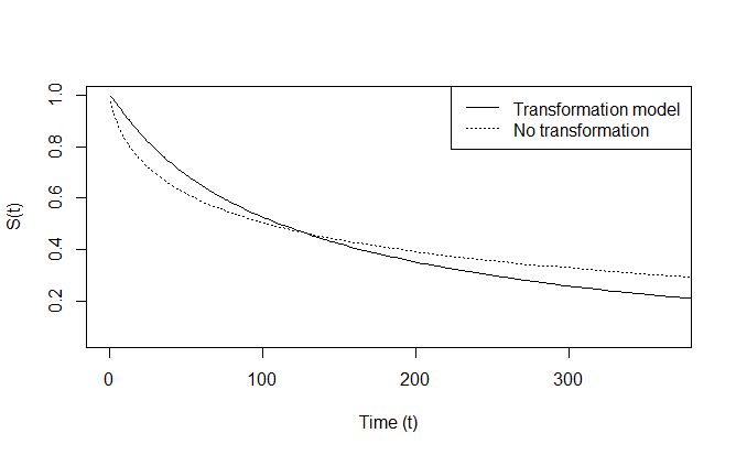
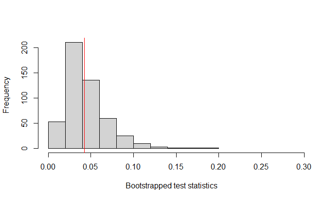
Figure 1: Top panel: the estimated survival curves using the two-step estimator with (solid curve) and without (dotted curve) transforming the response. Bottom panel: the bootstrap distribution of the goodness-of-fit test statistic.

7 Extension to competing risks

7.1 The model

Define $r$ latent times $T^{1},\ldots,T^{r}$. In this notation, assume that $T^{1},\ldots,T^{k}$ represent the competing risks, while $T^{k+1},\ldots,T^{r}$ represent possibly dependent censoring variables. Furthermore, like before, let $A$ represent administrative censoring, independent of $(T^{1},\ldots,T^{r})$. Since competing risks are assumed, suppose that $2\leq k\leq r$. All times are again represented on the log-scale. The extended model can then be written as:

$$\Lambda_{\theta_{j}}(T^{j})=X^{\top}\beta_{j}+Z\alpha_{j}+V\lambda_{j}+\epsilon_{j},\qquad j=1,\ldots,r.$$

Here $X=(1,\tilde{X}^{\top})^{\top}$ is a vector of exogenous covariates, $Z$ an endogenous variable, continuous or binary, and $V=g_{\gamma}(Z,W)$ a control function as defined before. Again $W=(1,\tilde{X}^{\top},\tilde{W})^{\top}$ where $\tilde{W}$ denotes a scalar binary or continuous instrumental variable. The error terms $(\epsilon_{1},\ldots,\epsilon_{r})$ are assumed to be multivariate normally distributed with mean equal to zero and with positive definite variance-covariance matrix $\Sigma$. Define the observed follow-up time $Y=\min(T^{1},\ldots,T^{r},A)$ and the indicator $\Delta^{*}=(\Delta_{1},\ldots,\Delta_{r},\Delta_{a})$ with $\Delta_{j}=\mathbbm{1}(Y=T^{j})$ for $j=1,\ldots,r$ and $\Delta_{a}=\mathbbm{1}(Y=A)$. The observed data are independent and identically distributed realisations $(Y_{i},\Delta^{*}_{i},W_{i},Z_{i})$ for $i=1,\ldots,n$. The following assumptions will be made in addition to Assumptions (A7) and (A8):

1. $(\epsilon_{1},\ldots,\epsilon_{r},A)\perp\!\!\!\perp(W,Z)$.

2. $(T^{1},\ldots,T^{r})$ and $A$ are conditionally independent, given $(W,Z)$.

3. The covariance matrix of $(\tilde{X}^{\top},Z,V)$ has full rank as well as $\text{Var}(\tilde{W})$ is strictly larger than zero.

4. The probabilities $P(Y=T^{j}|W,Z)$ for $j=1,\ldots,r$ and $P(Y=A|W,Z)$ are strictly positive.

5. Administrative censoring by $A$ is non-informative for $(T^{1},\ldots,T^{r})$ given $W$ and $Z$.

In order to define the likelihood function, some useful sub-distributions can be defined, conditional on $W=w=(1,\tilde{x}^{\top},\tilde{w})^{\top}$ and $Z=z$. Denote the parameter vector

$$\eta=(\beta_{1}^{\top},\ldots,\beta_{r}^{\top},\alpha_{1},\ldots,\alpha_{r},\lambda_{1},\ldots,\lambda_{r},\sigma_{1},\ldots,\sigma_{r},\rho_{12},\ldots,\rho_{(r-1)r},\theta_{1},\ldots,\theta_{r})^{\top}.$$

To ease notation, define:

$$b_{T^{j}}=\Lambda_{\theta_{j}}(y)-x^{\top}\beta_{j}-z\alpha_{j}-g_{\gamma}(z,w)\lambda_{j}$$

and

$$\tau_{j}=x^{\top}\beta_{j}+z\alpha_{j}+g_{\gamma}(z,w)\lambda_{j}.$$

We can then derive:

$$\begin{split}&f_{Y,\Delta^{*}|W,Z}(y,1,0,\ldots,0|w,z,\gamma;\eta)\\[5.0pt] &\quad=\frac{1}{\sigma_{1}}\bar{\Phi}\biggl{(}\frac{\Lambda_{\theta_{2}}(y)-m_{2.1}}{s_{2.1}},\ldots,\frac{\Lambda_{\theta_{r}}(y)-m_{r.1}}{s_{r.1}};\rho_{23.1},\ldots,\rho_{(r-1)r.1}\biggl{)}\phi\biggl{(}\frac{b_{T^{1}}}{\sigma_{1}}\biggl{)}\\ &\qquad\times\Lambda_{\theta_{1}}^{\prime}(y)P(A>y),\end{split}$$

where for $j=2,\ldots,r$:

$$m_{j.1}=x^{\top}\beta_{j}+z\alpha_{j}+g_{\gamma}(z,w)\lambda_{j}+\rho_{1j}\frac{\sigma_{j}}{\sigma_{1}}\bigl{(}\Lambda_{\theta_{1}}(y)-x^{\top}\beta_{1}-z\alpha_{1}-g_{\gamma}(z,w)\lambda_{1}\bigl{)}$$

and

$$s_{j.1}=\sigma_{j}(1-\rho_{1j}^{2})^{1/2}.$$

Moreover, for $2\leq j<q\leq r$:

$$\rho_{jq.1}=\frac{\rho_{jq}-\rho_{1j}\rho_{1q}}{\biggl{\{}(1-\rho_{1j}^{2})(1-\rho_{1q}^{2})\biggl{\}}^{1/2}}.$$

Furthermore, $\bar{\Phi}(t_{2},\ldots,t_{r};\rho_{23.1},\ldots,\rho_{(r-1)r.1})$ is the complementary cumulative distribution function of a random vector $(Y_{2},\ldots,Y_{r})$ following a $(r-1)$-variate normal distribution with mean zero, unit variances and covariance between $Y_{j}$ and $Y_{q}$ equal to $\rho_{jq.1}$ for $2\leq j<q\leq r$. The formulas for the sub-densities of $(Y,\Delta^{*})$ given $(W,Z)$ when $\Delta_{j}=1$ for $j=2,\ldots,r$ can be derived similarly.

Finally, when $A$ is observed, i.e. $\Delta_{a}=1$, it can be derived that:

$$f_{Y,\Delta^{*}|W,Z}(y,0,\ldots,0,1|w,z,\gamma;\eta)=\bar{\Phi}\biggl{(}b_{T^{1}},\ldots,b_{T^{r}};\Sigma\biggl{)}f_{A}(y),$$

where $\bar{\Phi}$ is the tail distribution function of $(\epsilon_{1},\ldots,\epsilon_{r})$ with variance-covariance matrix $\Sigma$ as defined before. Under very similar assumptions as before, a two-step procedure can be used to estimate the model parameters. In a second step, using the obtained estimated $\hat{\gamma}$, the following likelihood function will therefore be maximized:

$$\hat{L}(\hat{\gamma},\eta)$$

$$\quad=\prod_{i=1}^{n}\biggl{\{}\prod_{j=1}^{r}\bar{f}_{Y,\Delta^{*}|W,Z}(y_{i},\Delta_{i}^{*}|w_{i},z_{i},\hat{\gamma};\eta)^{\Delta_{ij}}\biggl{\}}\bar{f}_{Y,\Delta^{*}|W,Z}(y_{i},\Delta_{i}^{*}|w_{i},z_{i},\hat{\gamma};\eta)^{\Delta_{ia}},$$

with $\bar{f}_{Y,\Delta^{*}|W,Z}(y_{i},\Delta_{i}^{*}|w_{i},z_{i},\hat{\gamma};\eta)$ being $f_{Y,\Delta^{*}|W,Z}(y_{i},\Delta_{i}^{*}|w_{i},z_{i},\hat{\gamma};\eta)$ without the density and distribution function of $A$ since the administrative censoring is assumed to be non-informative.

More information about the necessary assumptions and derivation of the likelihood can be found in Section G of the Supplementary Material. In the framework of competing risks, the cumulative incidence function (CIF) is often calculated. In the presence of $k$ competing events, the function is defined by: $I_{j}(t|W,Z)=P(T\leq t,D=j|W,Z)$ where $T=\min(T^{1},\ldots,T^{k})$ and $D=j$ if $T=T^{j}$ for $j=1,\ldots,k$. Hence, it can be interpreted as the probability of failing from cause $j$ before time $t$, in the presence of the other competing events. For the first cause of failure, this becomes:

$$\begin{split}&I_{1}(t|w,z)\\[5.0pt] &\quad=\int_{-\infty}^{t}{}\frac{1}{\sigma_{1}}\bar{\Phi}\biggl{(}\frac{\Lambda_{\theta_{2}}(e)-m_{2.1}}{s_{2.1}},\ldots,\frac{\Lambda_{\theta_{k}}(e)-m_{k.1}}{s_{k.1}};\rho_{23.1},\ldots,\rho_{(k-1)k.1}\biggl{)}\\ &\qquad\times\phi\biggl{(}\frac{\Lambda_{\theta_{1}}(e)-\tau_{1}}{\sigma_{1}}\biggl{)}\Lambda_{\theta_{1}}^{\prime}(e)de\end{split}$$

with $\bar{\Phi}(\cdot)$ the tail distribution of a $(k-1)$-variate normal distribution with mean equal to zero, variances equal to one and correlations equal to $\rho_{jq.1}$ for $2\leq j<q\leq k$. The quantities $m_{j.1},s_{j.1}$ and $\rho_{jq.1}$ are defined as before. Similarly, the cumulative incidence function for the other causes can easily be calculated.

7.2 Simulation study

To evaluate the finite sample performance of this proposed estimator, another simulation study is performed. A data set of size $1000$ is simulated $500$ times. We consider two competing risks and one dependent censoring time. The performance of three different estimators is compared based on the estimated cumulative incidence function. The three compared estimators are: the two-step estimator, the naive estimator and a nonparametric estimator. For the two-step estimator, the cumulative incidence function can be calculated as explained in the Supplementary Material. The naive estimator differs from the two-step estimator by ignoring the endogeneity of the variable $Z$. For this estimator, the CIF can be calculated in the same way but removing all terms related to the control function $V=g_{\gamma}(Z,W)$. The nonparametric estimator of the CIF assumes independent censoring (but no independence between the competing risks) as explained by Aalen et al., (2008). This nonparametric CIF can be calculated using the function cuminc of the R-package cmprsk. The three estimators are compared with the expected CIF, which can be calculated using the formula of the CIF of the two-step estimator but using the true parameters instead of estimates.

A comparison of the cumulative incidence functions is done in terms of the empirical mean and root mean squared error (RMSE) at different time points. If we denote by $I(t)$ the expected value of the CIF at time $t$ and by $\hat{I}^{j}(t)$ the estimated value of a specific estimator in iteration $j$, the RMSE of this estimator at time $t$ is defined by:

$$\text{RMSE(t)}=\sqrt{500^{-1}\sum_{j=1}^{500}{\bigl{[}\hat{I}^{j}(t)-I(t)\bigl{]}^{2}}}.$$

To enable a more thorough comparison of the RMSEs, a global RMSE measure is calculated as well:

$$\int_{1}^{t_{\max}}{RMSE(t)dt}.$$

More details about the simulation study as well as the results can be found in Section G.4 of the Supplementary Material. From these results, we can see that the empirical means of the CIF are always very close to the expected value $I(t)$ for the two-step estimator. On the contrary, the empirical means of the CIF estimated using the naive estimator and nonparametric estimator can be much more deviant from the expected value. Looking at the RMSE, this value is the smallest for the two-step estimator for all considered time points. Especially for larger time points, it can be seen that the two-step estimator outperforms the naive and nonparametric estimator. Also, the global RMSE measure is lowest for the two-step estimator in all considered scenarios in the simulation study. Moreover, the plots we made to compare the estimated CIF with the expected CIF showed that the results of the two-step estimator are very close to the expected CIF. It can clearly be seen that the naive estimator deviates much more from the expected CIF than the two-step estimator. Finally, it can be observed that in some scenario’s, the two-step estimator also clearly outperforms the nonparametric estimator. Hence, accounting for dependent censoring as well as confounding is again important.

7.3 Data application

The proposed model is now applied to the Health Insurance Plan of Greater New York experiment (Shapiro,, 1997). The data have previously been analysed by Beyhum et al., (2023), among others. The clinical trial was designed to investigate to effect of periodic screening on breast cancer mortality rates. The study lasted from 1963 until 1986 and followed $60695$ women between the age of $40$ and $64$. All participants were randomly assigned to either the control group ($\tilde{W}=0$) or the intervention group ($\tilde{W}=1$). The members of the intervention group were offered an initial screening as well as three subsequent annual screens. However, not all women of the intervention group participated in the screening. In total, $30130$ women were assigned to the intervention arm but $9984$ of them refused screening. We define $Z=1$ for women who actually participated in the screening and $Z=0$ otherwise. Because of the noncompliance rate of about $33\%$, the women in group $Z=1$ might exhibit different characteristics from the women in group $Z=0$ (see Shapiro, (1997)). Hence, $Z$ is included as an endogenous variable and $\tilde{W}$ can be used as an instrumental variable. Note that in this study, noncompliance is only recorded in one direction. Indeed, people are allowed to refuse screening but women assigned to the control group are not allowed to participate in the screening. Therefore, we will specify the reduced form by $Z=\mathbbm{1}(X^{\top}\gamma>\nu)\times\tilde{W}$ and calculate the control function accordingly. We will also include the standardized age of the participants when they enter the study as an exogenous covariate.

In this study, two competing risks are considered: (log) time until death due to breast cancer ($T^{1}$) and (log) time until death due to other causes ($T^{2}$). Note that the main interest is the causal effect of $Z$ on $T^{1}$. Censoring occurs because some subjects are lost to follow-up or alive at the end of the study. We will assume that independent censoring ($A$) is the only type of censoring. Hence, the observed follow-up time is $Y=\min(T^{1},T^{2},A)$. As the model assumptions require, it will be assumed that $T^{1}$ and $T^{2}$ are bivariate normal, conditionally on the covariates. In contrast to Beyhum et al., (2023), we use a parametric approach, which enables us to estimate the effect of the treatment, as well as the effect of the continuous covariate age.

Our two-step estimator will be compared with a naive estimator, ignoring the endogeneity of $Z$ and hence not including a control function. The results can be found in Table 4. The effect of screening on the time until death from breast cancer is estimated to be significant at the 5% level using the naive estimator but insignificant when accounting for endogeneity. As can be expected, screening has no effect on dying from other causes when accounting for endogeneity. However, the naive model estimates this effect to be highly significant. The fact that the estimated effect using the naive model is about $10$ times larger than the estimated effect obtained from our two-step estimator suggests that the baseline risk of dying from other causes is higher amongst the women who refused the screening compared to women who participated. A possible explanation could be that, in general, women who refused screening are less likely to go to a doctor compared to women who participated. It can also be seen that age is highly significant for dying from other causes than breast cancer, while not significant for dying from breast cancer. Figure 2 shows the estimated CIFs for a woman that is $50$ years old and (1) participated in the screening (dotted black curve), (2) was selected but did not participate (solid grey curve) and (3) was assigned to the control group (solid black curve). In this figure, you can again see that women who refused screening have the highest risk of dying from other causes. Women who participated in the screening have the lowest risk of dying from breast cancer. However, this effect is estimated to be non-significant at the 5% level. All of these results are in line with the findings by Beyhum et al., (2023).

Two-step estimator Naive model Est. St. d. $p$ Est. St. d. $p$ $\beta_{T1,0}$ 76.950 0.107 0.000 76.739 1.345 0.000 $\beta_{T1,\text{age}}$ -0.728 0.165 0.082 -0.741 0.215 0.001 $\alpha_{T1}$ 0.898 0.485 0.064 1.091 0.476 0.022 $\lambda_{T1}$ -0.137 0.121 0.255 $\beta_{T2,0}$ 63.650 9.818 0.000 62.916 9.595 0.000 $\beta_{T2,\text{age}}$ -4.517 0.806 0.000 -4.501 0.795 0.000 $\alpha_{T2}$ 0.255 0.302 0.399 2.402 0.475 0.000 $\lambda_{T2}$ -1.517 0.309 0.000 $\sigma_{T1}$ 14.344 0.464 0.000 14.297 0.373 0.000 $\sigma_{T2}$ 14.656 2.854 0.000 14.699 2.561 0.000 $\rho$ 0.000 0.546 1.000 0.020 0.025 0.417 $\theta_{1}$ 2.000 0.026 0.000 2.000 0.011 0.000 $\theta_{2}$ 2.000 0.082 0.000 2.000 0.081 0.000

Table 4: Estimation results for the two-step and naive estimator. Given are the parameter estimate, estimated standard error and $p$-value.

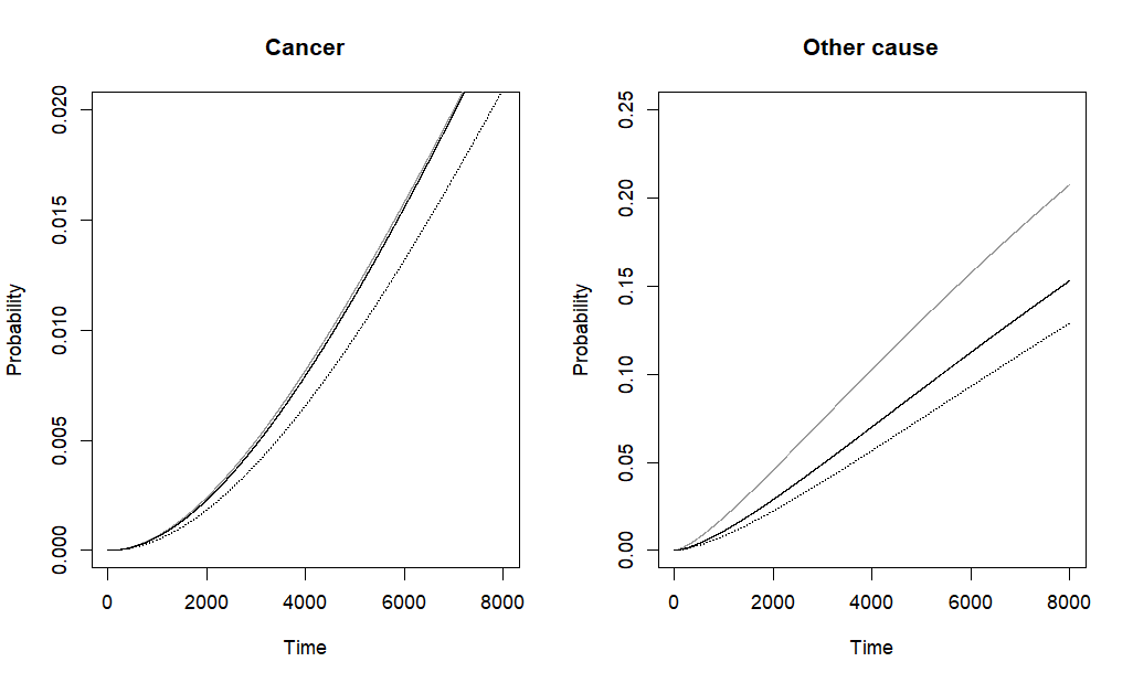
Figure 2: The estimated CIF for different groups. We make a distinction between women who were selected and participated (dotted black curves), women who were selected but did not participate (solid grey curves) and the control group (solid black curves).

References

- Aalen et al., (2008) Aalen, O., Borgan, O., and Gjessing, H. (2008). Survival and Event History Analysis: A Process Point of View. Springer.
- Aldrich and Nelson, (1991) Aldrich, J. H. and Nelson, F. D. (1991). Linear probability, logit, and probit models. Quantitative applications in the social sciences 45. Sage, Beverly Hills, 10th print edition.
- Azzalini and Valle, (1996) Azzalini, A. and Valle, A. (1996). The multivariate skew normal distribution. Biometrika, 83(4):175–726.
- Basu and Ghosh, (1978) Basu, A. and Ghosh, J. (1978). Identifiability of the multinormal and other distributions under competing risks model. Journal of Multivariate Analysis, 8(3):413–429.
- Beyhum et al., (2023) Beyhum, J., Florens, J.-P., , and Van Keilegom, I. (2023). A nonparametric instrumental approach to confounding in competing risks models. Lifetime data analysis, 29(4):709–734.
- Beyhum et al., (2022) Beyhum, J., Florens, J.-P., and Van Keilegom, I. (2022). Nonparametric instrumental regression with right censored duration outcomes. Journal of business & economic statistics, 40(3):1034–1045.
- Blanco et al., (2020) Blanco, G., Chen, X., Flores, C. A., and Flores-Lagunes, A. (2020). Bounds on average and quantile treatment effects on duration outcomes under censoring, selection, and noncompliance. Journal of business & economic statistics, 38(4):901–920.
- Bloom et al., (1997) Bloom, H. S., Orr, L. L.and Bell, S. H., Cave, G., Doolittle, F., Lin, W., and Bos, J. M. (1997). The benefits and costs of JTPA title II-A programs: Key findings from the national job training partnership act study. The Journal of Human Resources, 32(3):549–576.
- Box and Cox, (1964) Box, G. E. and Cox, D. R. (1964). An analysis of transformations. Journal of the Royal Statistical Society Series B: Statistical Methodology, 26(2):211–243.
- Braekers and Veraverbeke, (2005) Braekers, R. and Veraverbeke, N. (2005). A copula-graphic estimator for the conditional survival function under dependent censoring. Canadian Journal of Statistics, 33(3):429–447.
- Centorrino and Florens, (2021) Centorrino, S. and Florens, J.-P. (2021). Nonparametric estimation of accelerated failure-time models with unobservable confounders and random censoring. Electronic journal of statistics, 15(2):5333–5379.
- Crommen et al., (2024) Crommen, G., Beyhum, J., and Van Keilegom, I. (2024+). An instrumental variable approach under dependent censoring. Test (forthcoming).
- Czado and Van Keilegom, (2023) Czado, C. and Van Keilegom, I. (2023). Dependent censoring based on parametric copulas. Biometrika, 110(3):721–738.
- (14) Deresa, N. W. and Van Keilegom, I. (2020a). Flexible parametric model for survival data subject to dependent censoring. Biometrical Journal, 62(1):136–156.
- (15) Deresa, N. W. and Van Keilegom, I. (2020b). A multivariate normal regression model for survival data subject to different types of dependent censoring. Computational Statistics & Data Analysis, 144:106879.
- Deresa and Van Keilegom, (2024) Deresa, N. W. and Van Keilegom, I. (2024+). Copula based Cox proportional hazards models for dependent censoring. Journal of the American Statistical Association (forthcoming).
- Deresa et al., (2022) Deresa, N. W., Van Keilegom, I., and Antonio, K. (2022). Copula-based inference for bivariate survival data with left truncation and dependent censoring. Insurance: Mathematics and Economics, 107:1–21.
- Efron and Tibshirani, (1998) Efron, B. and Tibshirani, R. J. (1998). An introduction to the bootstrap. Monographs on statistics and applied probability 57. Chapman and Hall/CRC, Boca Raton.
- Emoto and Matthews, (1990) Emoto, S. E. and Matthews, P. C. (1990). A Weibull model for dependent censoring. The Annals of Statistics, 18(4):1556–1577.
- Emura and Chen, (2016) Emura, T. and Chen, Y.-H. (2016). Gene selection for survival data under dependent censoring: A copula-based approach. Statistical methods in medical research, 25(6):2840–2857.
- Frandsen, (2015) Frandsen, B. R. (2015). Treatment effects with censoring and endogeneity. Journal of the American Statistical Association, 110(512):1745–1752.
- Huling et al., (2019) Huling, J. D., Yu, M., and O’Malley, A. J. (2019). Instrumental variable based estimation under the semiparametric accelerated failure time model. Biometrics, 75(2):516–527.
- Kaplan and Meier, (1958) Kaplan, E. L. and Meier, P. (1958). Nonparametric estimation from incomplete observations. Journal of the American Statistical Association, 53(282):457–481.
- Khan and Tamer, (2009) Khan, S. and Tamer, E. (2009). Inference on endogenously censored regression models using conditional moment inequalities. Journal of econometrics, 152(2):104–119.
- Li et al., (2015) Li, J., Fine, J., and Brookhart, A. (2015). Instrumental variable additive hazards models. Biometrics, 71(1):122–130.
- Navarro, (2010) Navarro, S. (2010). Control Functions, pages 20–28. Palgrave Macmillan UK, London.
- Newey and McFadden, (1994) Newey, W. K. and McFadden, D. (1994). Large sample estimation and hypothesis testing. Elsevier.
- Rivest and Wells, (2001) Rivest, L.-P. and Wells, M. T. (2001). A martingale approach to the copula-graphic estimator for the survival function under dependent censoring. Journal of Multivariate Analysis, 79(1):138–155.
- Robins and Finkelstein, (2000) Robins, J. M. and Finkelstein, D. M. (2000). Correcting for noncompliance and dependent censoring in an AIDS clinical trial with inverse probability of censoring weighted (IPCW) log-rank tests. Biometrics, 56(3):779–788.
- Sant’Anna, (2021) Sant’Anna, P. H. (2021). Nonparametric tests for treatment effect heterogeneity with duration outcomes. Journal of Business & Economic Statistics, 39(3):816–832.
- Shapiro, (1997) Shapiro, S. (1997). Periodic screening for breast cancer: the hip randomized controlled trial. JNCI Monographs, 1997(22):27–30.
- Sujica and Van Keilegom, (2018) Sujica, A. and Van Keilegom, I. (2018). The copula-graphic estimator in censored nonparametric location-scale regression models. Econometrics and Statistics, 7:89–114.
- Tchetgen et al., (2015) Tchetgen, E. J. T., Walter, S., Vansteelandt, S., Martinussen, T., and Glymour, M. (2015). Instrumental variable estimation in a survival context. Epidemiology (Cambridge, Mass.), 26(3):402–410.
- Tsiatis, (1975) Tsiatis, A. (1975). A nonidentifiability aspect of the problem of competing risks. Proceedings of the National Academy of Sciences - PNAS, 72(1):20–22.
- Wooldridge, (2010) Wooldridge, J. M. (2010). Econometric Analysis of Cross Section and Panel Data. MIT press.
- Yeo and Johnson, (2000) Yeo, I. and Johnson, R. A. (2000). A new family of power transformations to improve normality or symmetry. Biometrika, 87(4):954–959.
- Zheng and Klein, (1995) Zheng, M. and Klein, J. P. (1995). Estimates of marginal survival for dependent competing risks based on an assumed copula. Biometrika, 82(1):127–138.