A Wideband Distributed Massive MIMO Channel Sounder for Communication and Sensing

Abstract

Channel sounding is a vital step in understanding wireless channels for the design and deployment of wireless communication systems. In this paper, we present the design and implementation of a coherent distributed massive MIMO channel sounder operating at 5-6 GHz with a bandwidth of 400 MHz based on the NI USRP X410. Through the integration of transceiver chains and RF switches, the design facilitates the use of a larger number of antennas without significant compromise in dynamic capability. Our current implementation is capable of measuring thousands of antenna combinations within tens of milliseconds. Every radio frequency switch is seamlessly integrated with a 16-element antenna array, making the antennas more practical to be transported and flexibly distributed. In addition, the channel sounder features real-time processing to reduce the data stream to the host computer and increase the signal-to-noise ratio. The design and implementation are verified through two measurements in an indoor laboratory environment. The first measurement entails a single-antenna robot as transmitter and 128 distributed receiving antennas. The second measurement demonstrates a passive sensing scenario with a walking person. We evaluate the results of both measurements using the super-resolution algorithm SAGE. The results demonstrate the great potential of the presented sounding system for providing high-quality radio channel measurements, contributing to high-resolution channel estimation, characterization, and active and passive sensing in realistic and dynamic scenarios.

I Introduction

Coherent transmission and reception from a massive number of distributed antennas is the foundation of emerging technologies such as distributed massive multiple-input multiple-output (MIMO) and cell-free massive MIMO [1, 2, 3, 4, 5, 6, 7, 8]. These technologies hold the potential to enhance capacity, reliability, localization accuracy and sensing capability. Expanding the number of antennas raises the upper limit on the spatial degrees of freedom of the channel, which could lead to a significant increase in capacity and to higher diversity orders. Compared to the conventional MIMO with antennas in a compact area, separating or distributing the antennas makes the system less prone to large-scale fading effects. The distributed nature of the antennas also opens up more opportunities for utilizing the channel information for integrated sensing and communication (ISAC) applications, as the number of physical anchor points increases.

In order to propose practical solutions and evaluate the system’s performance, it is essential to attain a thorough understanding of the distributed massive MIMO channels. Consequently, there is a need to design a channel sounder that can capture the real-world propagation characteristics. The channel sounder should have a large number of antennas that can be flexibly distributed, a large bandwidth to obtain high delay resolution, and a high snapshot rate to characterize dynamic scenarios. Moreover, the propagation channels among different base station (BS) antennas, besides the traditional BS-user links, become increasingly important to be understood. For example, in distributed MIMO systems, channel state information between BS antennas can facilitate calibration procedures that enable coherent transmission and reception [9]. Similarly, in ISAC, such channel information can be utilized to detect changes in the environment. Therefore, the channel sounder must be capable of measuring the channels between all combinations of antennas in the system, also known as multi-node or multi-link channel sounding [10, 11, 12]. Lastly, it is imperative for a channel sounder cost-effective in its implementation and easy to deploy in various scenarios.

In the literature, there are three main ways to increase the number of antennas of a channel sounder: i) increasing the number of transceiver chains, ii) employing radio frequency (RF) switches or iii) through the virtual array principle. Several channel sounders have been presented in [13, 14, 15, 16, 17, 18, 19] that feature one receiver chain per antenna. The primary limitations of this approach include the increase in cost with the number of antennas, the potential complexity arising from the substantial data generated by the RF chains, and the risk of the sounder becoming cumbersome and unwieldy. In addition, it can be challenging to perform phase calibration of the transceiver chains, which is needed for angle-of-departure (AoD) and angle-of-arrival (AoA) estimation. Nevertheless, a solution was presented in [18] utilizing a custom-made calibration unit. Channel sounders employing the switched array principle, e.g. [20, 21, 22], can address these drawbacks. However, they must compromise on dynamic capability. Furthermore, the integration of parallel RF channels with RF switches, as shown in [22], presents a viable trade-off solution. Channel sounders that employ the virtual array principle [23] – a convenient and cost-effective method to measure the channel with an immense number of antennas lack dynamic capability.

The bandwidth of a channel sounder is limited by the underlying RF equipment. Channel sounders based on a vector network analyzer (VNA) [24] can have a bandwidth on the order of several GHz. However, VNAs measure the channel much slower than other solutions and hence limit the dynamic capability. Therefore, many channel sounders are based on software-defined radios [13, 17, 18, 14, 20, 12] such as the USRP series from National Instruments, and custom designs [15, 22, 25, 21]. While customs design are typically with high-cost [15, 22], software-radios can offer a complete radio system without a high development cost. Naturally, the bandwidth of the channel sounder is limited by the specifications of the state-of-the-art commercially available SDRs. One also has to consider the data rate between an SDR and the host computer, which can easily become several gigabytes per second in (ultra-)wideband setups. When bandwidth is increased, real-time processing on the SDR might be needed to reduce the data rate between the SDR and the host computer.

To the best our knowlegde, a channel sounder combing the multi-link capability with a large number of antennas and a large bandwidth has not previously been presented in the literature. Nevertheless, such a channel sounder opens up opportunities to enhance distributed MIMO channel models, phase calibration techniques, localization algorithms and ISAC methods. To fill this gap, we present the design, implementation and verification of a scalable multi-link distributed massive MIMO channel sounder operating in the 5$-$6 GHz range with an instantaneous bandwidth up to 400 MHz based on the NI USRP X410. The sounder is capable of measuring the channels between thousands of antenna combinations in tens of milliseconds. The main contributions of this work are:

• Through the integration of both parallel RF chains and RF switches, we facilitate the utilization of a larger number of antennas without significant compromise in dynamic capability. Every SP16T RF switch is seamlessly integrated with a 16-element antenna array within a single panel. This integration streamlines the calibration process in an anechoic chamber, guaranteeing phase coherency among the co-located antennas.

• The high data rate problem, due to the 400 MHz bandwidth, is addressed with real-time processing on the field-programmable gate array (FPGA), selecting and averaging sounding frames. As a result, we realize high processing gains without increasing the data rate.

• The design and implementation of the channel sounder are verified by two sample measurements in an indoor laboratory environment. The two measurements are tailored for a communication application and a sensing application, respectively, where the potential of distributed MIMO is also well demonstrated.

An early version of the channel sounder, which could only measure a simple single-input single-output link, has been presented in [26]. It is worth noting that our design and implementation is open-source [27], based on open-source tool chains, built with off-the-shelf electronic components, allowing other researchers to build a similar channel sounder.

The rest of the paper is organized as follows. Sect. II discusses the channel sounder design and implementation. Sect. III elaborates on the post-processing and calibration aspects. In Sect. IV, the two sample measurements and the results that demonstrate the capability of the sounder and the potential of distributed MIMO in communication and sensing are included. Finally, conclusive remarks are summarized in Sect. V.

Notations: Throughout this paper, italic letters are used to represent scalars. Bold lowercase letters are for vectors and bold uppercase letters for matrices or tensors. The vector denoted as $\mathbf{1}$ consists of elements that are all equal to one and has proper length. $(\cdot)^{\rm T}$ indicates matrix transposition, $\mathrm{j}=\rm\sqrt{-1}$, $\mathrm{Tr}(\cdot)$ denotes the trace operator, and $\otimes$ represents Kronecker product. $|\cdot|$ and $\angle$ denote the absolute value and the argument of a complex number, respectively. In addition, $\mathrm{max}\{\cdot\}$ and $\mathrm{sum}\{\cdot\}$ denote the maximum value and the sum of all the elements in a vector, respectively.

II Design and Implementation

II-A High-level Design

Fig. 1 presents a basic block diagram of the channel sounder. Core components include one or more NI USRP X410 and a host computer. Optionally, a Rubidium clock, Global Positioning System (GPS) antenna, and an RF switch can be integrated into the setup. The NI USRP X410 is a four-channel full-duplex SDR. It has a tunable center frequency ranging from 1 MHz to 7.2 GHz and supports instantaneous bandwidths up to 400 MHz. This device uses the Xilinx Ultrascale+ RFSoC ZU28DR FPGA, for which we developed custom code. We implemented channel sounding functions using a custom signal processing block within the RF network on chip (RFNoC) open source framework that manages the streaming and processing of RF data on the FPGA. It also allows for the design of custom applications with RFNoC blocks. Our processing block can selectively average received samples, optimizing the data stream to the host computer and improving the signal-to-noise ratio (SNR).

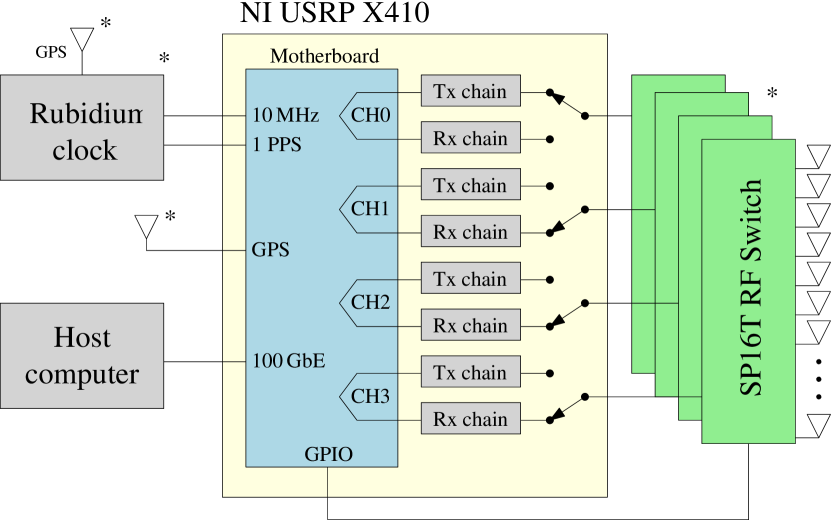
Figure 1: Simplified block diagram of the channel sounder. Components indicated with * are optional.

The Rx and Tx chains are connected to the same port through an internal RF switch which is controlled in real time by our custom block. This means that the respective port can transmit or receive, but not both at the same time. The following principle applies: when one transmitting, all the other transceiver chains in the channel sounder are receiving. Then, each port in the channel sounder transmits after one another in a pre-configured order.

The USRP is connected to a host computer via an Ethernet interface. Depending on the data rate requirements between the host and the USRP, the 100 GbE interface or the 1 GbE interface can be utilized. Note that multiple USRPs can be connected to one host computer. Apart from the appropriate Ethernet interface, there is no strict hardware requirement for the host computer. However, the host computer has to be fast enough to handle and store the stream of data from the USRP, which can vary from about 1 MB/s to hundreds of MB/s, depending on the configuration.

Rubidium clocks provide a stable time and frequency synchronization between two or more USRPs without the need for any cabling between them during the measurement, allowing for mobile measurements. Note however that the Rubidium clocks have to be synchronized via a cable before the actual measurements. Sufficient synchronization can also be achieved with the GPS disciplined oscillator built into the USRP and an external GPS antenna if the measurement scenario allows for stable GPS reception.

The external RF switches allow for a cost-effective extension of the number of channels that can be measured, enhancing the spatial resolution of the propagation measurements. Their states are real-time and independently controlled by our custom RFNoC block through the general-purpose input/output (GPIO) ports of the USRP. We have implemented the following time-division multiple access (TDMA) scheme to control the state of the switches. There are in total $N_{\mathrm{RF}}$ RF chains in the system, with $\mathbf{n_{\mathrm{T}}}\in\mathbb{N}^{N_{\mathrm{RF}}\times 1}$ containing the number of (switched) antennas connected to the RF chains in the transmission mode, and $\mathbf{n_{\mathrm{R}}}\in\mathbb{N}^{N_{\mathrm{RF}}\times 1}$ containing the number of switched channels for different RF chains in the receiving mode. Only one antenna is transmitting at a time. While one antenna is transmitting, the other antennas, except those connected to the same USRP port, are receiving and the RF switches are being switched until all channels have been measured. After that, the next antenna transmits, etc. The total number of channels that can be measured is

$$\textbf{1}^{\mathrm{T}}(\textbf{n}_{\mathrm{T}}\otimes\textbf{n}_{\mathrm{R}})-\mathrm{Tr}(\textbf{n}_{\mathrm{T}}\textbf{n}^{\mathrm{T}}_{\mathrm{R}})$$ (1)

including reciprocal channels. The total unique number of channels is

$$\frac{1}{2}\,\textbf{1}^{\mathrm{T}}(\textbf{n}_{\mathrm{T}}\otimes\textbf{n}_{\mathrm{R}})-\frac{1}{2}\,\mathrm{Tr}(\textbf{n}_{\mathrm{T}}\textbf{n}^{\mathrm{T}}_{\mathrm{R}}).$$ (2)

Because of the simultaneous reception on different RF chains, the amount of time slots needed to measure all the antenna combinations is less than the amount of combinations. In our implementation, the total number of time slots it takes to measure the configured channels is $\max\{\mathbf{n_{\mathrm{R}}}\}\,\mathrm{sum}\{\textbf{n}_{\mathrm{T}}\}.$ At the time of writing, our implementation of the channel sounder contains three USRP X410, three host computers, three Rubidium clocks, and eight Mini-Circuits USB-1SP16T-83H SP16T RF switches. This makes it possible to measure to measure 7686 unique channels.

II-B Elementary Sounding Frame

The principle of channel sounding is as follows: a known waveform is transmitted at the desired carrier frequency. On the receiver side, the received waveform is processed to obtain the channel transfer function and impulse response. This could be done for all antenna combinations to recover the directional properties of the channel. For the design of the channel sounding waveform, it is important that the waveform has a large bandwidth, a uniform power-spectral density, and high energy [28]. A large bandwidth allows us to achieve a high delay resolution, while the uniform power-spectral density allows us to estimate the channel at across the whole bandwidth with the same quality. Higher energy means a higher SNR. Since the peak power of the transmit power amplifier is limited, high energy implies a low peak-to-average-power ratio (PAPR) of the sounding waveform should be used. It is convenient to resort to the frequency domain to design the sounding waveform as a multi-tone signal. Such a waveform, $\textbf{s}\in\mathbb{C}^{L\times 1}$ with a length of $L$ samples, can in discrete complex baseband be expressed as

$$\textbf{s}(n)=\frac{1}{L}\sum_{k=0}^{L-1}\textbf{x}(k)\exp\left(\mathrm{j}2\pi kn/L\right),$$ (3)

where $\textbf{x}\in\mathbb{C}^{L\times 1}$ contains the complex amplitudes for all the tones. The entries of x can now be chosen so that $|\textbf{x}(k)|=1$ for the bandwidth of interest and $\angle\,\textbf{x}(k)$ optimizes the PAPR. For our channel sounder, we choose a Zadoff-Chu sequence for $\textbf{x}(k)$ since $|\textbf{x}(k)|=1$ and its (inverse) Fourier transform, if the sequence length is a prime number, is also a Zadoff-Chu sequence, which has good time-continuous PAPR and autocorrelation properties [29, 30].

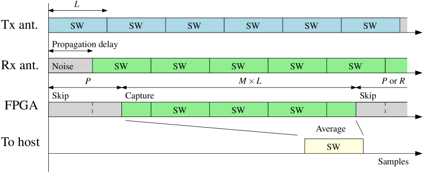
Figure 2: RFNoC processing block functionality for one channel snapshot. SW stands for sounding waveform.

During a single-channel snapshot, the respective transmitter sends multiple repetitions of the same sounding waveform s with a length of $L$ samples, as illustrated in Fig. 2. Note that to avoid aliasing, $L$ should be longer than

$$L\geq\frac{\Delta\tau_{\mathrm{max}}}{T_{\mathrm{s}}},$$ (4)

where $\Delta\tau_{\mathrm{max}}$ is the maximum delay difference between the first and last received multipath component, and $T_{\mathrm{s}}$ is the sample period. These signals then propagate through the radio channel and arrive at the receiver with an unknown propagation delay. Therefore, samples have to be discarded according to this propagation delay. Otherwise, a couple of samples will be averaged with noise, which reduces the signal-to-noise ratio. In addition, another $\frac{\Delta\tau_{\mathrm{max}}}{T_{\mathrm{s}}}$ samples have to be discarded, so the received sounding signals are the result of a circular convolution between the channel impulse response and the original sounding signal. In general, this is not a strict requirement, yet quite convenient for post-processing. At the beginning of each elementary sounding frame, the RF switches are also configured for the respective antenna; this means that we also have to take into account the switching time of the RF switch. We define $P$ as the total number of samples that are discarded and its value should be higher than

$$P\geq\frac{\tau_{\mathrm{0,max}}+\Delta\tau_{\mathrm{max}}+T_{\mathrm{sw}}}{T_{\mathrm{s}}},$$ (5)

where $\tau_{\mathrm{0,max}}$ the maximum delay of the first multipath component, and $T_{\mathrm{sw}}$ is the maximum time it takes for RF switch to switch channel. The switching time also takes into account the delay of the cable from the GPIO output of the USRP to the RF switch. If RF switches are only used for receiving, then the requirement for $P$ could be reduced,

$$P\geq\mathrm{max}\left(\frac{\tau_{\mathrm{0,max}}+\Delta\tau_{\mathrm{max}}}{T_{\mathrm{s}}},\frac{T_{\mathrm{sw}}}{T_{\mathrm{s}}}\right).$$ (6)

In practice, $P$ can be set higher than required to account for possible time synchronization errors between receiver and transmitter. After disregarding $P$ samples, $M$ waveforms of length $L$ are captured and averaged, as illustrated in Fig. 2. Averaging is done by averaging each $i^{\mathrm{th}}$ sample of each received sounding signal. Let us represent the $m^{\mathrm{th}}$ received waveform as $\mathbf{y}_{m}\in\mathbb{C}^{L\times 1}$, where $m\in[1,M]$. Then the processed received waveform $\mathbf{y}\in\mathbb{C}^{L\times 1}$ becomes

$${\textbf{y}}(i)=\frac{1}{2^{K}}\sum^{M}_{m=1}{\textbf{y}_{m}}(i),$$ (7)

where $i$ indicates the $i^{\mathrm{th}}$ element of the vectors, and $K\in\mathbb{N}$ is the parameter for the division factor in the averager. This division is a power of two by design because this simplifies the logic design. The processed signal is then sent to the host for channel estimation and storage. In the meantime, the RFNoC blocks skips $P$ or $R$ samples until it starts to capture the signal of the next channel. $P$ samples are skipped if the next received signal comes directly after the previous signal. $R$ can be used to adjust the interval $T_{\mathrm{rep}}$ at which the entire channel is measured. $R$ can be calculated as:

$$R=\left\lceil\frac{T_{\mathrm{rep}}}{T_{\mathrm{s}}}\right\rceil-\max\{\mathbf{n_{\mathrm{R}}}\}\,\mathrm{sum}\{\textbf{n}_{\mathrm{T}}\}(P+ML)+P.$$ (8)

Typical values for the parameters introduced above are presented in Table II.

II-C Implementation

The functionality that was introduced in the previous subsection has been implemented by means of custom logic design on the FPGA of the X410 and an C++ application on the host computers. These were developed within the open-source RFNoC framework provided by Ettus Research. This framework allows for time-efficient development through so-called RFNoC blocks, similar to the GNU Radio structure. The framework takes care of synchronization, clock generation, data streaming, and analog front-end configuration. By default, each block has an input and output port for both data and control packets. The interface is based on the AXI-Stream protocol. Detailed discussion about the RFNoC framework is beyond the scope of this manuscript and can be found in the USRP Hardware Driver and USRP Manual [31]. The complete FPGA implementation, including all the RFNoC blocks, is called an image. Our image is based on the “X4_400” image flavor (UHD v4.2.0.1) and includes two radio blocks, one replay block, and our custom channel sounding block. The radio block is the source and destination block for the RF data and is connected to both the replay block and the channel sounding block. The replay block is an existing block from the RFNoC library and is used to transmit the sounding waveform. With the replay block, we can download our sounding waveform to the DRAM of the X410 and then start transmitting it at the appropriate time. When the onboard DRAM is used to transmit the sounding signal, there is no transfer of sample data between the host computer and the USRP. Hence, the 1 GbE Ethernet interface could be used to connect the USRP and the host computer if the USRP would only be used as transmitter or if the receiver data rate is low.

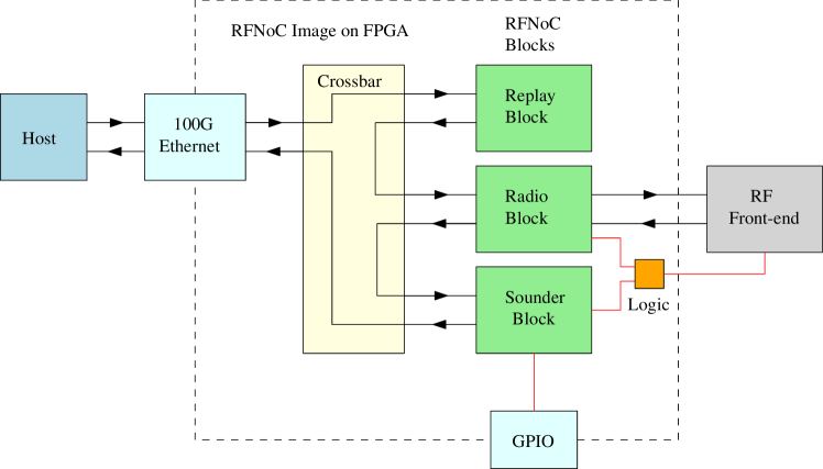
Figure 3: RFNoC image on the FPGA of the USRP X410.

The channel sounding block is responsible for discarding samples, block-averaging the received waveforms, and controlling the RF switches. The respective samples are discarded by a logic circuit based on a set of counters that can override the valid signal of the AXI-Stream protocol. The non-discarded samples then go to the block averager. Since the data type is complex short, the averaging can efficiently be done by bit-wise right shifting real and imaginary each sample $K$ times and then adding the $i^{\mathrm{th}}$ sample of each sounding signal. The simplified circuit diagram of the averager is shown in Fig. 4. The averager consists of an arithmetic shifter, block RAM (BRAM), and an adder. Multiplexers are controlled by a counter for $m=\{1,2,\ldots,M\}$. 1) If $m=1$: Samples are added with zero and saved in the BRAM. 2) $1<m<M$: The $i$-th sample comes in and the $i$-th sample is fetched out of the memory, and their sum is stored in the memory. 3) $m=M$: The $i$-th sample comes in, and the $i$-th sample is fetched from the memory. The sum of those samples is presented at the output of the block averager. In the special case of $m=M=1$, the $i$-th sample is presented directly on the output of the averager.

Figure 4: Simplified circuit diagram of the averager within the SounderRx block.

Due to the high sample rate, four samples are being processed per clock cycle, resulting in a memory width of 128 bits. While the sample counter for the averager is enabled by the valid signal of the incoming samples, the counters and logic that control the RF switches (both for the external and internal Tx/Rx switches) are enabled by the rx_running or tx_running logic signal to ensure the correct timing. These signals are the main on/off signals for the transmitter and receiver chain. The clock driving this RFNoC block is clk_radio, of which the frequency is equal to 125 MHz.

To store sample data and configure the USRP, a C++ application has been developed that utilizes the UHD library (Release v4.2.0.1), containing all the essential software to control the USRPs. An additional C++ library was also developed to set the parameters ($L$, $P$, $K$, $M$, $R$, $\mathbf{n}_{\mathrm{T}}$, $\mathbf{n}_{\mathrm{R}}$) belonging to the RFNoC block.

II-D Synchronization

The USRPs are synchronized via a 1 pulse per second (1PPS) signal for time synchronization and a 10 MHz reference signal for frequency synchronization. Through the main application on the host computer, the synchronization source can be set to either a GPS disciplined oscillator or an external clock (e.g., Rubidium clock). The channel sounder is designed to start on the positive flank of a 1PPS. To eliminate the requirement that two or more USRPs start at the same 1PPS flank, the repetition time $T_{\mathrm{rep}}$ must be chosen in such a way that at each PPS flank a sounding signal starts transmitting, e.g., $T_{\mathrm{rep}}$ = 50 ms. In this way, multiple USRPs can start at different 1PPS flanks; hence, no communication is needed between them. Nevertheless, the USRPs can also start on the same 1PPS flank via the GPS time when the system is synchronized with GPS.

II-E Antenna Design

Our implementation comprises eight mini-circuit USB-1SP16T-83H RF switches. For each RF switch, we designed a rectangular $2\times 4$ antenna array with each element having two ports for horizontal and vertical polarization. The geometric centers of the antennas are separated by 26.7 mm $\approx 0.5\lambda$. Other dimensions can be found in Fig. 5. Each element of the array is a proximity-coupled stacked patch antenna and is designed to operate in the 5.0-6.0 GHz frequency range (S11 $<-10$ dB). The antenna is made with Rogers Corp. RO4350B laminate. The antennas are mounted on top of the RF switch inside a plastic box, forming one antenna panel. A photograph of one antenna panel is shown in Fig. 6. All panels have been characterized in an anechoic chamber, which is also needed to perform high-resolution angular estimation of multipath components. Fig. 7 presents the complete radiation pattern for antenna element 7 of a panel at 5.675 GHz for both polarizations, showing a typical pattern of a patch antenna. It should be noted that the gain given in the figures includes switch losses and internal cable losses.

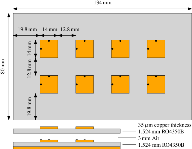
Figure 5: Dimensions of the 16-element antenna array.

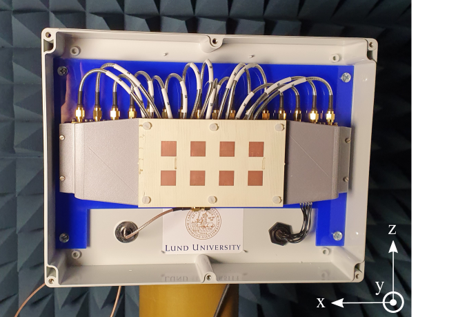
Figure 6: Photograph of one antenna panel in the anechoic chamber.

Figure 7: Full measured radiation pattern of vertically-polarized antenna element 7 on panel 0 at 5.675 GHz. The plot shows a typical pattern for a patch antenna. The peak gain value, including cable and RF switch losses is -0.4 dBi.

II-F Final Specifications, Performance and Link Budget

We summarize the channel sounder specifications in Table I. Typical parameters for three scenarios and their corresponding performance metrics in are presented in Table II. As shown, the channel sounder can be tailored for wide variety of measurement scenarios and different application requirements. While Scenarios 1 and 2 are further discussed in Section IV, more information about Scenario 3 can be found in [32].

While most of the calculations are straight-forward, special attention should be paid to the calculation of the maximum Doppler frequency. From the sampling theorem, it is known that the maximum Doppler frequency of the channel should be smaller than half of the sampling frequency. In our channel sounder three frequencies could be regarded as the sampling frequency: i) the snapshot rate or the repetition frequency, which has historically been used for the maximum Doppler frequency calculation for channel sounders [28], ii) the frequency at which each antenna combination is measured [30], applied in systems with a large amount of switched antennas, iii) the baseband sampling frequency $f_{\mathrm{s}}$, the fundamental limit. For cases ii) and iii) the channel is not continuously measured but rather in bursts. If the Doppler frequency is much lower than the sampling frequencies, it might not be possible to estimate the Doppler frequency because the phase difference between the samples is much smaller than the noise component of the signal. Hence, the maximum Doppler frequency should be carefully calculated based on the configuration of the channel sounder and the application scenario. In addition, the average functionality of our channel sounder poses an extra limitation on the Doppler frequency. If we repeat the same waveform $\textbf{s}\in\mathbb{C}^{L\times 1}$ $M$ times and virtually introduce a Doppler frequency offset $\nu$, the averaged waveform $\textbf{y}\in\mathbb{C}^{L\times 1}$ becomes:

$$\mathbf{y}(i) =\frac{1}{2^{K}}\sum^{M}_{m=1}\mathbf{s}(i)\exp(\mathrm{j}2\pi\nu(mLT_{\mathrm{s}}+iT_{\mathrm{s}}))$$

$$=\frac{1}{2^{K}}\,\mathbf{s}(i)\exp(\mathrm{j}2\pi\nu iT_{\mathrm{s}})\sum^{M}_{m=1}\exp(\mathrm{j}2\pi\nu mLT_{\mathrm{s}}).$$ (9)

The summation in (9) is a sum of phasors. If the phases of these phasors do not align well, e.g. due to a high Doppler frequency, this sum can attenuate the signal drastically. We consider

$$\nu_{\mathrm{max}}\leq\dfrac{0.1f_{\mathrm{s}}}{ML}$$ (10)

to be an acceptable limit. In addition, it must be noted that the processing gain does not include the beamforming gain because it depends on the AoD and AoD.

TABLE I: Final specifications of the channel sounder

Specification	Value
Type	Hybrid-switched
Operating frequency	5$-$6 GHz
Bandwidth	400 MHz
Number of antenna panels	8
Panel array configuration	2$\times$4 dual polarized
Panel azimuth/elevation 10 dB beamwidths	120/120 degrees
Number of standalone antennas	4
Maximum number of antenna combinations	7656
Maximum RF switch frequency	50 kHz
Typical snapshot rate	10$-$200 Hz
Typical output power	18 dBm
ADC/DAC depth	12/14 bits

TABLE II: Typical configuration of the channel sounder and corresponding performance metrics

Description	Parameter	Scenario 1	Scenario 2	Scenario 3
Center frequency	$f_{\mathrm{c}}$	5.675 GHz	5.675 GHz	5.6 GHz
Sample frequency	$f_{\mathrm{s}}$	500 Msps	500 Msps	500 Msps
Sounding waveform length	$L$	1024	1024	8192
Number of tones	$F$	819	819	4095
Number of waveforms to sum in averager	$M$	8	8	64
Division of $2^{K}$ in averager	$K$	3	3	2
Skipped samples	$P$	9216	9216	49152
Skipped samples	$R$	2221472	14348416	1975712
Number of RF chains	$N_{\mathrm{RF}}$	9	8	2
Total number of transmit antennas	$\mathrm{sum}\{\textbf{n}_{\mathrm{T}}\}$	1	128	1
Maximum amount of panel antennas	$\mathrm{max}\{\textbf{n}_{\mathrm{R}}\}$	16	16	1
Metric	Equation
Bandwidth	$f_{\mathrm{s}}F/L$	400 MHz	400 MHz	250 MHz
Snapshot rate $f_{\mathrm{rep}}=1/T_{\mathrm{rep}}$	$f_{\mathrm{s}}/(\mathrm{sum}\{\textbf{n}_{\mathrm{T}}\}\mathrm{max}\{\textbf{n}_{\mathrm{R}}\}(P+ML)+R)$	200 Hz	10 Hz	200 Hz
Coherence time	$\mathrm{sum}\{\textbf{n}_{\mathrm{T}}\}\mathrm{max}\{\textbf{n}_{\mathrm{R}}\}(P+ML)/f_{\mathrm{s}}$	557 $\mu$s	71 ms	2 ms
Antenna combinations	see (2)	128	7168	1
Max. delay spread	$L/f_{\mathrm{s}}$	2 $\mu$s	2 $\mu$s	16 $\mu$s
Max. Doppler frequency	$\mathrm{min}\left(f_{\mathrm{rep}}\,\text{or}\,\dfrac{f_{\mathrm{s}}}{P+ML},\dfrac{0.1f_{\mathrm{s}}}{ML}\right)$	29 kHz	29 kHz	100 Hz
Processing gain (w/o beamforming gain)	$10\,\log_{10}(ML)$	39 dB	39 dB	57 dB
Sensitivity level (20 dB SNR)	$-147.5+10\,\log_{10}(f_{\mathrm{s}}FM)$	-100 dBm	-100 dBm	-118 dBm
Data rate USRP to host (w/o overhead)	$\dfrac{4f_{\mathrm{s}}L\,\mathrm{sum}\{\textbf{n}_{\mathrm{T}}\}\mathrm{max}\{\textbf{n}_{\mathrm{R}}\}N_{\mathrm{RF,USRP}}}{\mathrm{sum}\{\textbf{n}_{\mathrm{T}}\}\mathrm{max}\{\textbf{n}_{\mathrm{R}}\}(P+ML)+R}$	236 MB/s	671 MB/s	3.2 MB/s

A link budget analysis is presented in Fig. 8 of a single antenna as transmitter and a panel as receiver. Note that the noise figure is dependent on the receiver gain setting on the USRP and temperature-variant. The noise figure given in the figure is a typical value under maximum gain configuration.

Figure 8: Link-budget analysis of a standalone antenna as transmitter to one antenna panel as receiver.

III Post-processing and calibration

The output data of the channel data can be represented as a six-dimensional tensor $\textbf{D}(s,p_{\mathrm{T}},p_{\mathrm{R}},m_{\mathrm{T}},m_{\mathrm{R}},n)$, where $s$ is the snapshot index, $n_{\mathrm{T}}$ the transmit chain index, $n_{\mathrm{R}}$ the receive chain index, $m_{\mathrm{T}}$ the transmit antenna index, $m_{\mathrm{R}}$ the receive antenna index, and $i$ the sample index. Further data processing is done by performing a Discrete Fourier Transform over $i$ to obtain $\textbf{Y}(s,p_{\mathrm{T}},p_{\mathrm{R}},m_{\mathrm{T}},m_{\mathrm{R}},k)$ where $k$ is the frequency index. Hereafter, the frequency indices are selected where a signal was transmitted, i.e. $\textbf{x}(k)\neq 0$. The complete channel response H is then calculated by diving Y by x in the frequency domain:

$$\textbf{H}(s,p_{\mathrm{T}},p_{\mathrm{R}},m_{\mathrm{T}},m_{\mathrm{R}},k)=\dfrac{\textbf{Y}(s,p_{\mathrm{T}},p_{\mathrm{R}},m_{\mathrm{T}},m_{\mathrm{R}},k)}{\textbf{x}(k)}.$$ (11)

Note that H includes the response of the RF chains and the antennas, which is not part of the propagation channel. Although this result could already be used for some simulations, our ultimate goal is to obtain the true propagation characteristics. This can be done by modeling the propagation channel as a superposition of specular multipath components, which each have the following parameters: delay ($\tau$), Doppler frequency ($\nu$), azimuth and elevation AoD ($\phi_{\mathrm{T}}$, $\theta_{\mathrm{T}}$), azimuth and elevation AoA ($\phi_{\mathrm{R}}$, $\theta_{\mathrm{R}}$), and complex polarimetric path gains ($\boldsymbol{\gamma}$). In addition, it is assumed that these geometrical propagation parameters of MPCs are unchanged during the observation time of $S$ snapshots. Analytically,

$$\begin{split}&\textbf{H}(s,p_{\mathrm{T}},p_{\mathrm{R}},m_{\mathrm{T}},m_{\mathrm{R}},k)\\ =&\sum_{l=1}^{L}\textbf{a}_{m_{\mathrm{R}},p_{\mathrm{R}}}^{\mathrm{T}}(\phi_{\mathrm{R},l},\theta_{\mathrm{R},l},f_{k})\begin{pmatrix}\gamma_{\mathrm{HH},l}&\gamma_{\mathrm{HV},l}\\ \gamma_{\mathrm{VH},l}&\gamma_{\mathrm{VV},l}\\ \end{pmatrix}\\ &\textbf{a}_{m_{\mathrm{T}},p_{\mathrm{T}},}(\phi_{\mathrm{T},l},\theta_{\mathrm{T},l},f_{k})\textbf{b}_{p_{\mathrm{T}},n_{\mathrm{R}}}(k)\exp(-\mathrm{j}2\pi f_{k}\tau_{l})\\ &\exp(\mathrm{j}2\pi\nu_{l}t_{s,p_{\mathrm{T}},p_{\mathrm{R}},m_{\mathrm{T}},m_{\mathrm{R}}})+\textbf{N}(s,p_{\mathrm{T}},p_{\mathrm{R}},m_{\mathrm{T}},m_{\mathrm{R}},f_{k}),\end{split}$$ (12)

where $f_{k}$ is the absolute frequency value that corresponds with frequency index $k$, $l$ is the index of the MPC, $t_{s,p_{\mathrm{T}},p_{\mathrm{R}},m_{\mathrm{T}},m_{\mathrm{R}}}$ gives the time in seconds when the channel between the respective antenna elements was measured, N gives the measurement noise. Parameters $\gamma_{\mathrm{HH},l},\gamma_{\mathrm{HV},l},\gamma_{\mathrm{VH},l},\gamma_{\mathrm{VV},l}$ denote the horizontal-to-horizontal, horizontal-to-vertical, vertical-to-horizontal, and vertical-to-vertical polarization gains of the $l$-th MPC. Moreover, $\textbf{a}_{m_{\mathrm{T}},p_{\mathrm{T}}}\in\mathbb{C}^{2\times 1}$ and $\textbf{a}_{m_{\mathrm{R}},p_{\mathrm{R}}}\in\mathbb{C}^{2\times 1}$ denote the polarimetric antenna responses. These antenna responses are obtained through the effective aperture distribution function (EADF) [33, 34] based on the antenna panel calibration data. Furthermore, $\textbf{b}_{p_{\mathrm{T}},p_{\mathrm{R}}}$ contains the frequency response of the sounder without antennas, which can be obtained from a back-to-back measurement with an attenuator. Hence,

$$\textbf{b}_{p_{\mathrm{T}},p_{\mathrm{R}}}(k)=\dfrac{\textbf{Y}(0,p_{\mathrm{T}},p_{\mathrm{R}},0,0,k)}{\textbf{x}(k)\textbf{s}_{21,\mathrm{att}}(k)},$$ (13)

where $\textbf{s}_{21,\mathrm{att}}\in\mathbb{C}^{F\times 1}$ is the frequency response of the attenuator measured with a VNA. Note that due to the design of the channel sounder, it is not possible to measure the response between the transmit and receive chains on the same channel, i.e. $n_{\mathrm{T}}\neq n_{\mathrm{R}}$. Measurement of all RF channel combinations can be cumbersome and time consuming. $N_{\mathrm{RF}}(N_{\mathrm{RF}}-1)/2$ connections have to be made. To decrease this amount, it is possible to obtain all combinations $\textbf{b}_{p_{\mathrm{T}},p_{\mathrm{R}}}$ by measuring only a set of combinations, which needs $2(N_{\mathrm{RF}}-2)+1$ back-to-back connections. Analytically,

$$\textbf{b}_{p_{\mathrm{T}},p_{\mathrm{R}}}(k)=\dfrac{\textbf{b}_{0,p_{\mathrm{R}}}(k)\textbf{b}_{p_{\mathrm{T}},1}(k)}{\textbf{b}_{0,1}(k)}.$$ (14)

Several approaches exist to estimate the MPC parameters $(\tau,\nu,\phi_{\mathrm{T}},\theta_{\mathrm{T}},\phi_{\mathrm{R}},\theta_{\mathrm{R}},\boldsymbol{\gamma})$ such as expectation-maximization (EM)[35], space-alternating generalized expectation maximization (SAGE) [36, 37], and RIMAX [33]. To process our verification measurements in Section IV, we have implemented and applied the SAGE algorithm.

IV Verification and Measurements

IV-A Scenario 1: Uplink Measurement

In order to verify the functionality of the channel sounder, we have performed a measurement of the propagation channel at 5.675 GHz between a single antenna robot and eight distributed panels in an indoor laboratory environment with a bandwidth of 400 MHz. The laboratory room, depicted in Fig. 9, measures approximately 5 meters by 12 meters, of which an area of 5 meters by 6 meters was used for the measurements. Eight panels were distributed in the room in groups of two, as illustrated in Fig. 10. Each group of two panels was vertically stacked at heights of 0.92 m and 1.84 m. Then each group of four panels was connected to a USRP X410 through 10 m long LMR400 RF cables and custom-made cables for switch control. The two USRPs were connected to an industrial computer through a link 100 GbE and are synchronized through one Rubidium clock.

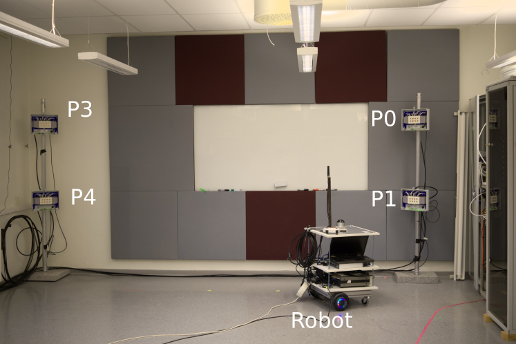
Figure 9: Photograph of the measurement setup and environment. Four of the eight panels (P3, P4, P0, P1) are visible: two on the left and two on the right. The robot is located in front of the panels.

Figure 10: Floor plan of the measurement environment and the trajectory for the uplink measurement given in red.

Figure 11: Narrowband channel gain at 5.675 GHz for a single vertically-polarized antenna per panel and the result after performing maximum ratio combining (MRC) of all 128 antennas.

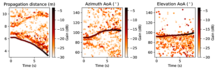
Figure 12: High-resolution parameter estimates of the MPCs seen from P0 using the SAGE algorithm for the first eight seconds of the uplink channel measurement. From left to right: propagation distance, azimuth AoA, elevation AoA.

The robot is equipped with a USRP X410, a wideband dipole antenna, two regular laptops, a Rubidium reference clock, uninterruptible power supply (UPS), a light detection and ranging (lidar) sensor and an inertial measurement unit (IMU). A laptop was responsible for controlling the USRP and the movement of the robot. The other laptop was used to collect data from the lidar and IMU, which provide ground truth information about the location of the robot and the panels in the room via a simultaneous localization and mapping (SLAM) algorithm. Reflective tape was applied to the panels to enhance their visibility in the lidar scan. The robot is an in-house design based on a hoverboard and is controlled via a game controller over Bluetooth. A detailed list of primary equipment can be found in Table III.

TABLE III: Primary equipment

Device	Amount	Model
Software-defined radio	3	NI USRP X410
Industrial computer	1	Advanctech MIC-770 V2
Dipole antenna	1	Taoglas TU.60.3H31
Rubidium clock	2	SRS FS725 & SRS FS740
Lidar	1	Ouster OSDome (128 lines)
IMU	1	Microstrain 3DM-GX5-25 (AHRS)
RF switches (panel)	8	Mini-Circuits USB-1SP16T-83H

During the measurement, the robot followed a round trajectory, maintaining a LoS connection with all panels, as illustrated in Fig. 10. The channel sounder configuration during this measurement can be found in Table II.

Fig. 11 presents the narrowband channel gains during the measurement for several vertically polarized antenna elements at different panels, and the channel gain after applying maximum ratio combining (MRC) for all 128 antennas. It can be observed that with MRC the overall channel gain increased. The deep small-scale fading experienced by every single antenna has also been effectively mitigated. This demonstrates the potential for the reliability increase with distributed massive MIMO systems. Furthermore, the SAGE algorithm is applied to extract the parameters of the MPCs observed by panel 0 are depicted in Fig. 12 for the initial eight seconds of measurement. The LoS component is readily apparent. In the propagation distance plot, we discern two additional tracks of MPCs. The track closest to the LoS emanates from reflections off the ceiling and ground. The other track, exhibiting increasing propagation distance, is most likely a reflection off one of the side walls of the room. These two tracks are also visible in the azimuth plot: the ground/ceiling reflections align closest to the LoS azimuth angle, while the other track ranges from around 77 degrees to about 70 degrees. Examining the elevation plot, we observe that MPCs originate primarily from the ceiling, attributable to the lighting infrastructure, causing significant scattering.

IV-B Scenario 2: Sensing Measurement

To demonstrate the sensing capability of our channel sounder, we have performed an additional measurement in the same environment as in Section IV-A. In contrast with the previous measurement, all eight panels are now configured as both transmitting and receiving. This configuration allows us to estimate the AoD from each panel, which can be useful for sensing purposes. The channel sounder configuration can be found in Tab. II under Scenario 2. The goal of this measurement was to test the capability of sensing a person with our channel sounder, based on the estimated parameters of the MPCs. During the measurement, a member of research group walked on the red line shown in Fig. 13 within a time of approximately 10 seconds. The person stood still at the beginning and at the middle of the walk. The SAGE estimation results of the propagation delay ($\tau$), azimuth AoD ($\phi_{\mathrm{T}}$) and AoA ($\phi_{\mathrm{R}}$) are presented in Fig. 14. The figures show that most of the estimates are not time-dependent because the panels and the environment are static, except for the walking person. However, we are interested in the MPCs that change with time because these could be related to the moving person. At 5 seconds in the AoD plot, a change in the AoD can be observed. To get a better observation of the dynamic MPCs, we have manually selected a parameter subspace $\{\tau=[29\,\mathrm{ns},32\,\mathrm{ns}],\phi_{\mathrm{R}}=[65^{\circ},110^{\circ}],\theta_{\mathrm{T}}=[70^{\circ},180^{\circ}]\}$. The MPCs in this subspace are marked with the blue line Fig. 14. To verify the MPCs in this subspace are linked to the moving person, we calculated the intersection between the AoD and the AoA, indicated with the blue crosses in Fig. 13. Because intersection points are in close proximity of the red line, we can confident that the MPCs are connected to the movement of the person.

Figure 13: Floor plan of the measurement environment. The walking trajectory of a person is given by the red line. The blue crosses are the intersections of the AoD from P3 and AoA of P1, after selecting a parameter subspace.

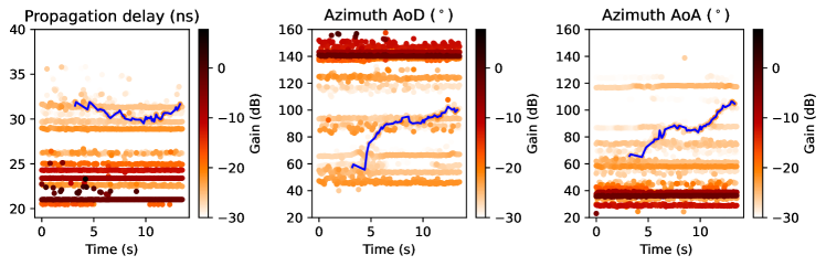
Figure 14: High-resolution parameter estimates of the MPCs between P1 (Rx) and P3 (Tx) using the SAGE algorithm during measurement scenario 2. From left to right: propagation delay, azimuth AoD, azimuth AoA

V Conclusions

In this paper we have presented the design, implementation and verification of a channel sounder for distributed massive MIMO based on open-source software and off-the-shelf electronic components. Our design utilized multiple NI USRP X410 and radio frequency switches as core components. By means of a flexible design, customized FPGA code, and integration of multiple parallel transceiver chains and RF switches, we were able to scale up the number of antennas in a cost-efficient way and without a significant compromise in dynamic capability. The combination of the high number of antennas, wide bandwidth and multi-link capability makes this design a valuable asset for conducting cutting-edge research within areas such as distributed massive MIMO and integrated sensing and communication. This potential was demonstrated through two measurement campaigns in our laboratory, one distributed massive MIMO uplink measurement and one passive sensing measurement.

References

- [1] H. Q. Ngo, A. Ashikhmin, H. Yang, E. G. Larsson, and T. L. Marzetta, “Cell-Free Massive MIMO Versus Small Cells,” IEEE Transactions on Wireless Communications, vol. 16, no. 3, pp. 1834–1850, Mar. 2017. [Online]. Available: https://ieeexplore.ieee.org/document/7827017
- [2] Özlem Tugfe Demir, E. Björnson, and L. Sanguinetti, “Foundations of user-centric cell-free massive MIMO,” Foundations and Trends® in Signal Processing, vol. 14, no. 3-4, pp. 162–472, 2021.
- [3] H. Q. Ngo, L.-N. Tran, T. Q. Duong, M. Matthaiou, and E. G. Larsson, “On the Total Energy Efficiency of Cell-Free Massive MIMO,” IEEE Transactions on Green Communications and Networking, vol. 2, no. 1, pp. 25–39, Mar. 2018.
- [4] E. Björnson and L. Sanguinetti, “Making Cell-Free Massive MIMO Competitive With MMSE Processing and Centralized Implementation,” IEEE Transactions on Wireless Communications, vol. 19, no. 1, pp. 77–90, Jan. 2020.
- [5] E. Björnson, L. Sanguinetti, H. Wymeersch, J. Hoydis, and T. L. Marzetta, “Massive MIMO is a reality—What is next?: Five promising research directions for antenna arrays,” Digital Signal Processing, vol. 94, pp. 3–20, Nov. 2019.
- [6] S. Hu, F. Rusek, and O. Edfors, “Beyond Massive MIMO: The Potential of Data Transmission With Large Intelligent Surfaces,” IEEE Transactions on Signal Processing, vol. 66, no. 10, pp. 2746–2758, May 2018.
- [7] G. Interdonato, E. Björnson, H. Quoc Ngo, P. Frenger, and E. G. Larsson, “Ubiquitous cell-free Massive MIMO communications,” EURASIP Journal on Wireless Communications and Networking, vol. 2019, no. 1, p. 197, Aug. 2019.
- [8] L. Van der Perre, E. G. Larsson, F. Tufvesson, L. D. Strycker, E. Björnson, and O. Edfors, “RadioWeaves for efficient connectivity: analysis and impact of constraints in actual deployments,” in 2019 53rd Asilomar Conference on Signals, Systems, and Computers, Nov. 2019, pp. 15–22, iSSN: 2576-2303.
- [9] E. G. Larsson and J. Vieira, “Phase Calibration of Distributed Antenna Arrays,” IEEE Communications Letters, vol. 27, no. 6, pp. 1619–1623, Jun. 2023.
- [10] C. Nelson, X. Li, T. Wilding, B. Deutschmann, K. Witrisal, and F. Tufvesson, “Large Intelligent Surface Measurements for Joint Communication and Sensing,” in 2023 Joint European Conference on Networks and Communications & 6G Summit (EuCNC/6G Summit), Jun. 2023, pp. 228–233.
- [11] S. Zelenbaba, D. Löschenbrand, M. Hofer, A. Dakić, B. Rainer, G. Humer, and T. Zemen, “A Scalable Mobile Multi-Node Channel Sounder,” in 2020 IEEE Wireless Communications and Networking Conference (WCNC), May 2020, pp. 1–6.
- [12] D. A. Wassie, I. Rodriguez, G. Berardinelli, F. M. L. Tavares, T. B. Sørensen, T. L. Hansen, and P. Mogensen, “An Agile Multi-Node Multi-Antenna Wireless Channel Sounding System,” IEEE Access, vol. 7, pp. 17 503–17 516, 2019.
- [13] D. Stanko, G. Sommerkorn, A. Ihlow, and G. D. Galdo, “Enable SDRs for Real-Time MIMO Channel Sounding featuring Parallel Coherent Rx Channels,” in 2022 IEEE 95th Vehicular Technology Conference: (VTC2022-Spring), Jun. 2022, pp. 1–5.
- [14] A. P. Guevara, S. De Bast, and S. Pollin, “Weave and Conquer: A Measurement-based Analysis of Dense Antenna Deployments,” in ICC 2021 - IEEE International Conference on Communications, Jun. 2021, pp. 1–6.
- [15] P. Laly, D. P. Gaillot, M. Lienard, P. Degauque, E. Tanghe, W. Joseph, and L. Martens, “Flexible real-time MIMO channel sounder for multidimensional polarimetric parameter estimation,” in 2015 IEEE Conference on Antenna Measurements & Applications (CAMA), Nov. 2015, pp. 1–3.
- [16] F. Euchner, M. Gauger, S. Doerner, and S. ten Brink, “A Distributed Massive MIMO Channel Sounder for “Big CSI Data”-driven Machine Learning,” in WSA 2021; 25th International ITG Workshop on Smart Antennas, Nov. 2021, pp. 1–6.
- [17] S. Malkowsky, J. Vieira, L. Liu, P. Harris, K. Nieman, N. Kundargi, I. C. Wong, F. Tufvesson, V. Öwall, and O. Edfors, “The World’s First Real-Time Testbed for Massive MIMO: Design, Implementation, and Validation,” IEEE Access, vol. 5, pp. 9073–9088, 2017.
- [18] D. Löschenbrand, M. Hofer, L. Bernadó, G. Humer, B. Schrenk, S. Zelenbaba, and T. Zemen, “Distributed Massive MIMO Channel Measurements in Urban Vehicular Scenario,” in 2019 13th European Conference on Antennas and Propagation (EuCAP), Mar. 2019, pp. 1–5.
- [19] D. Löschenbrand, M. Hofer, L. Bernadó, S. Zelenbaba, and T. Zemen, “Towards Cell-Free Massive MIMO: A Measurement-Based Analysis,” IEEE Access, vol. 10, pp. 89 232–89 247, 2022.
- [20] C. Nelson, X. Li, A. Fedorov, B. Deutschmann, and F. Tufvesson, “Distributed MIMO measurements for integrated communication and sensing in an industrial environment,” Sensors, vol. 24, no. 5, p. 1385, Feb. 2024.
- [21] J. Flordelis, G. Dahman, and F. Tufvesson, “Measurements of large-scale parameters of a distributed MIMO antenna system in a microcell environment At 2.6 GHz,” in 2013 7th European Conference on Antennas and Propagation (EuCAP), Apr. 2013, pp. 3026–3030.
- [22] P. Laly, D. Gaillot, G. Delbarre, M. V. d. Bossche, G. Vermeeren, F. Challita, E. Tanghe, E. Simon, W. Joseph, L. Martens, and M. Liénard, “Massive Radio Channel Sounder Architecture for 5G Mobility Scenarios: MaMIMOSA,” in 2020 14th European Conference on Antennas and Propagation (EuCAP), Mar. 2020, pp. 1–5.
- [23] M. Alatossava, A. Taparugssanagorn, V.-M. Holappa, and J. Ylitalo, “Measurement Based Capacity of Distributed MIMO Antenna System in Urban Microcellular Environment at 5.25 GHz,” in VTC Spring 2008 - IEEE Vehicular Technology Conference, May 2008, pp. 430–434.
- [24] T. Choi, P. Luo, A. Ramesh, and A. F. Molisch, “Co-Located vs Distributed vs Semi-Distributed MIMO: Measurement-Based Evaluation,” in 2020 54th Asilomar Conference on Signals, Systems, and Computers, Nov. 2020, pp. 836–841.
- [25] E. P. Simon, P. Laly, J. Farah, E. Tanghe, W. Joseph, and D. P. Gaillot, “Measurement of the V2I Channel in Cell-free Vehicular Networks with the Distributed MaMIMOSA Channel Sounder,” in 2023 17th European Conference on Antennas and Propagation (EuCAP), Mar. 2023, pp. 1–5.
- [26] M. Sandra, C. Nelson, and A. J. Johansson, “Ultrawideband USRP-Based Channel Sounding Utilizing the RFNoC Framework,” in 2022 IEEE Conference on Antenna Measurements and Applications (CAMA), Dec. 2022, pp. 1–3, iSSN: 2643-6795.
- [27] “Open USRP Channel Sounder.” [Online]. Available: https://github.com/michielsandra/openucs
- [28] A. F. Molisch, Wireless Communications, 2nd ed. Wiley Publishing, 2011.
- [29] D. Chu, “Polyphase codes with good periodic correlation properties (Corresp.),” IEEE Transactions on Information Theory, vol. 18, no. 4, pp. 531–532, Jul. 1972. [Online]. Available: https://ieeexplore.ieee.org/document/1054840
- [30] X. Cai, E. L. Bengtsson, O. Edfors, and F. Tufvesson, “A Switched Array Sounder for Dynamic Millimeter-Wave Channel Characterization: Design, Implementation and Measurements,” IEEE Transactions on Antennas and Propagation, 2023. [Online]. Available: http://lup.lub.lu.se/record/42028e8f-1ff7-413f-812c-61711bf66489
- [31] Ettus Research, “USRP Hardware Driver and USRP Manual.” [Online]. Available: https://files.ettus.com/manual/
- [32] M. Sandra, G. Tian, A. Fedorov, X. Cai, and A. J. Johansson, “Measurement-Based Wideband Maritime Channel Characterization,” The 17th European Conference on Antennas and Propagation (EuCAP 2023), 2023.
- [33] A. Richter, Estimation of Radio Channel Parameters: Models and Algorithms. ISLE, 2005.
- [34] X. Cai, M. Zhu, A. Fedorov, and F. Tufvesson, “Enhanced Effective Aperture Distribution Function for Characterizing Large-Scale Antenna Arrays,” IEEE Transactions on Antennas and Propagation, vol. 71, no. 8, pp. 6869–6877, Aug. 2023.
- [35] M. Feder and E. Weinstein, “Parameter estimation of superimposed signals using the EM algorithm,” IEEE Transactions on Acoustics, Speech, and Signal Processing, vol. 36, no. 4, pp. 477–489, Apr. 1988.
- [36] J. Fessler and A. Hero, “Space-alternating generalized expectation-maximization algorithm,” IEEE Transactions on Signal Processing, vol. 42, no. 10, pp. 2664–2677, Oct. 1994.
- [37] B. Fleury, M. Tschudin, R. Heddergott, D. Dahlhaus, and K. Ingeman Pedersen, “Channel parameter estimation in mobile radio environments using the SAGE algorithm,” IEEE Journal on Selected Areas in Communications, vol. 17, no. 3, pp. 434–450, Mar. 1999.