One-sided DI-QKD secure against coherent attacks over long distances

Abstract

Quantum Key Distribution (QKD) is a technique enabling provable secure communication but faces challenges in device characterization, posing potential security risks. Device-independent (DI) QKD protocols overcome this issue by making minimal device assumptions but are limited in distance because they require high detection efficiencies, which refer to the ability of the experimental setup to detect quantum states. It is thus desirable to find quantum key distribution protocols that are based on realistic assumptions on the devices as well as implementable over long distances. In this work, we consider a one-sided DI QKD scheme with two measurements per party and show that it is secure against coherent attacks up to detection efficiencies greater than 50.1% specifically on the untrusted side. This is almost the theoretical limit achievable for protocols with two untrusted measurements. Interestingly, we also show that, by placing the source of states close to the untrusted side, our protocol is secure over distances comparable to standard QKD protocols.

Quantum Key Distribution (QKD) is a technique that allows two remote users to establish a secure key over an untrusted quantum channel. This can be used to encrypt communication. QKD allows two parties to perform secure communication relying only on the laws of quantum mechanics and trusting that the devices they use follow a specific mathematical model [1, 2]. QKD is now commercially available and used for various applications. However, the challenge with QKD is that ensuring the quantum devices behave as expected is difficult, potentially opening security loopholes in the protocol [3, 4, 5, 6]. In response to these vulnerabilities, the concept of Device-Independent (DI) quantum key distribution emerges as a class of QKD protocols whose security can be proven with minimal assumptions about the devices [7, 8]. However, they are currently strongly limited in distance. This follows from the fact that they are much more sensitive than device-dependent protocols to photon losses, which in optical fibers scale exponentially with the distance.

To address these challenges, one possible approach is to incorporate well-chosen additional assumptions and ensure their validity. Many approaches have been proposed along these lines. These include Measurement-DI scenarios [9, 10], where two trusted parties send quantum states to a central untrusted measuring device, semi-DI scenarios based on dimension bounds [11, 12, 13, 14], and one-sided device-independent protocols (1SDI). A setting where only one party is trusted, can either be of the prepare-and-measure type [15, 16], where we trust the source, or of the entanglement-based type [17, 18, 19, 20, 21, 22, 23, 24], where we trust a measuring device. In general, entanglement-based 1SDI settings have an advantage over prepare-and-measure ones since they allow achieving long distances by placing the source close to the untrusted side, which is more sensitive to losses. In a prepare-and-measure scenario, the losses would need to be taken into account across the entire path from the source to the measuring device. For this reason, in this work, we consider an entanglement-based 1SDI scenario.

In our analysis, we assume that the source and one party’s device (Bob’s) are completely untrusted, while the second party’s device (Alice’s) is trusted. In particular, we assume that the trusted side measures two anti-commuting observables with a discrete number of outcomes and that the probability for a detector to click is independent of the basis choice (a.k.a. the fair-sampling assumption in the context of Bell experiments). This implies that rounds where she does not detect a photon can safely be discarded. As we do not make any assumption on the Hilbert space dimension or on the specific form of the measurements, we will say from now on that Alice’s device is semi-trusted. This framework, where only one party is untrusted while the second is (semi) trusted, is usually referred to as quantum steering [25]. From a real-world perspective, this scenario resembles a situation where a user needs to establish secure communication with a server. In this context, the device belonging to the server can be considered semi-trusted, as it is affiliated with a company that possesses the necessary resources and expertise to regularly test and validate their devices.

The robustness against photon losses of various forms of 1SDI QKD protocols with discrete variables have previously been explored in [19, 20, 22, 15, 16]. However, all these protocols are based on different forms of post-selection, where the secret key is derived only from specific measurement outcomes, discarding data from other rounds. Notably, in [20, 22, 15, 16], which are B92-like protocols, rounds yielding a particular outcome are discarded entirely. The use of protocols where certain outcomes coming from untrusted devices are discarded does not allow to prove security against the most general class of attacks in a device-independent scenario using the recently introduced Entropy Accumulation Theorem (EAT) framework of [26, 27, 28]. Moreover, it was shown in [29, 30] that protocols relying on post-selection are indeed sensitive to coherent attacks. As a result, the work by Branciard et al. [19], as mentioned by the same authors, is based on a security proof applicable against coherent attacks, only under the constraint that the devices do not retain memory from previous rounds, thus precluding consideration of fully untrusted parties. This limitation extends to subsequent works such as [22, 20]. More recently, Ioannou et al. [15, 16] studied a 1SDI prepare-and-measure setting, where the security was proven only against collective attacks. Notably, their class of protocols allows for the demonstration of security at detection efficiencies that can be relatively low. However, this setting, since it is of the prepare-and-measure type, does not allow to achieve secure communication over distances comparable to standard QKD protocols.

Figure 1: The scenario under consideration consists of an untrusted source preparing states $\rho$ and distributing them to both an untrusted measuring device (the black box), positioned near to the source, and a semi-trusted measuring device (the gray box), situated far from the source.

In this work, we explore a generalized entanglement-based version of the well-known BB84 protocol [31] and we demonstrate that, in the simple case where Bob represents the undetected quantum states as separate outcomes, our 1SDI QKD scheme is secure as long as Bob’s measurement has a detection efficiency greater than $50.1\%$ which is well within the current experimental limits. Interestingly, this threshold roughly corresponds to the one where any two-untrusted-measurements protocol becomes insecure [32]. Furthermore, as we do not perform any type of post-selection, one can analyze our protocols using the entropy-accumulation-theorem, allowing one to prove that our scheme is secure against coherent attacks. Finally, by placing a source of entangled photons close to Bob’s detector, we estimate that our 1SDI QKD protocol can be effectively implemented over distances of roughly $247$ km, assuming that Bob’s detectors and optical components have a total detection efficiency of $90\%$, that the visibility of the state prepared is of $99\%$, and that the detectors have a dark count rate of $p_{d}=10^{-6}$. All of these values have been achieved in a recent experiment on DI QKD [33].

1SDI scenario.— We will begin by outlining our setting, the additional assumptions we make beyond the standard assumptions made in DI QKD [8], and the protocol considered in this work.

Within this work, we have two spatially separated observers, Alice and Bob, who share a quantum state $\rho$ (Fig. 1). They perform measurements on their respective portions of the state corresponding to inputs $x,y$ and obtain outputs $a,b$ for Alice, Bob respectively. Alice’s and Bob’s measurements are represented as $M_{x}=\{M_{a|x}\}$ and $N_{y}=\{N_{b|y}\}$, respectively where $M_{a|x}$, $N_{b|y}$ are the measurement operators that are positive semi-definite and sum up to identity. The experiment’s observed correlations are characterized by a set of joint probability distributions or correlations, denoted as $\vec{p}=\{p(a,b|x,y)\}$. The observables of Alice and Bob are represented using the measurement operators as $A_{x}=M_{1|x}-M_{2|x}$ and $B_{y}=N_{1|y}-N_{2|y}$. The observables $A_{1}$, $A_{2}$ corresponding to Alice’s measurements are trusted to obey the relation:

$$\{A_{1},A_{2}\}=0.$$ (1)

In contrast, Bob’s measurement device is untrusted.

Figure 2: A model describing Alice’s device under the fair sampling assumption. A filter returns an output $D=\checkmark,\perp$ which is determined independently by the input $x$ and the state $\rho$. The detector performs a lossless measurement only if the filter returned $D=\checkmark$.

Let us remark here that, to account for no-detection events on Alice’s side, we will model her semi-trusted device inspired by [34]. Her device is composed of a filter and an ideal detector (Fig. 2). The filter outputs a flag $D=\checkmark,\perp$ based on whether her device produced a click or not. The filter is composed of two parts acting independently on the classical and quantum input. When they both accept the round, the device of Alice produces a click. If her device does not click, the round of the protocol gets discarded. If the filter produces a click $D=\checkmark$, Alice’s device performs one of the two ideal anti-commuting measurements according to the random input $x$ and obtains outcomes $a$. Making this assumption on Alice’s device is equivalent to performing an ideal measurement with unit efficiency. In contrast, if Bob fails to detect an incoming state, he stores a separate outcome as $b=\varnothing$.

Let us now describe the key distribution protocol.

1SDI QKD protocol: • An untrusted source prepares an entangled state $\rho$ which is distributed to Alice and Bob. • The two parties choose the measurements settings $x=1,2$ and $y=1,2$ according to a known distribution $p(x)$ and $p(y)$. • They obtain outcomes $a=1,2$, $D=\checkmark,\perp$, and $b=1,2,\varnothing$. The measurement settings and $D$ are announced publicly. If $D=\perp$, then the round is discarded. • Based on a random bit $T$, Alice and Bob decide if the round will be used to generate the secret key ($T=k$) in which case they store their outcomes, or to assess the security of the protocol ($T=t$) by revealing publicly their outcomes to estimate the probability distribution $\vec{p}$. • They use $\vec{p}$ to compute the key rate and decide whether to abort or not the protocol. • Finally, they perform error correction and privacy amplification.

An example of an honest implementation of the protocol is the case where Alice and Bob share a partially entangled state and perform the measurements of the observables $A_{1}=B_{1}=Z$ and $A_{2}=B_{2}=X$ and extract the secret key from the outcomes of the measurement of $Z$. The particular case where the state prepared is a maximally entangled state corresponds to an entanglement-based version of the BB84 protocol.

In a typical DI QKD scenario, the source of quantum states is placed in the middle between Alice and Bob and distributes two subsystems of an entangled state to the two parties. In this work, we consider a scenario (Fig. 1) where the untrusted source is positioned near Bob’s laboratory, a configuration previously explored in various contexts, e.g., [19, 35, 36, 37, 38]. This arrangement minimizes losses during the transmission of the state to Bob’s device, which is the one particularly sensitive to losses. The performance of Bob’s device is primarily affected by detector inefficiency. On Alice’s side, losses are less relevant as rounds with non-detection are simply discarded.

Key rate lower bounds.— The 1SDI QKD protocol described above satisfies the no-signaling condition of the generalized Entropy Accumulation Theorem [28]. This allows us to assess their security in the asymptotic case by verifying the positivity of the Devetak-Winter rate [39, 40]. When the secret key is extracted from Alice’s outcomes of the observables $A_{1}$ and Bob uses the outcomes of $B_{1}$ to reconstruct her string, the asymptotic key rate is given by

$$r_{\infty}\geq H(A_{1}|E)-H(A_{1}|B_{1}).$$ (2)

Here, we decided to extract the key by using one-way public communication from Alice to Bob. We make this choice because, as Alice’s device is semi-trusted, the convex-combination attacks as introduced in [41] do not apply to her device. Therefore, with this choice, we can achieve better key rates.

In eq. (2), $H(A_{1}|E)$ (or $H(A_{1}|B_{1})$) represents the conditional Von Neumann entropy of the outcomes of the measurement of $A_{1}$ given Eve’s information (or given the measurement outcomes of the observable $B_{1}$). As one can observe from (2), to find the asymptotic key rate, one needs to obtain the values of the conditional Von Neumann entropies $H(A_{1}|E)$ and $H(A_{1}|B_{1})$.

As far as $H(A_{1}|B_{1})$ is concerned, it can be estimated as

$$H(A_{1}|B_{1})=\sum_{a,b}p(a,b|1,1)\log_{2}\frac{p(a,b|1,1)}{p(b|1)}.$$ (3)

The above quantity can be directly inferred from the input-output statistics obtained through measurements of $A_{1}$ and $B_{1}$.

Let us now focus on $H(A_{1}|E)$. Here, we describe how to obtain a lower bound of $H(A_{1}|E)$ using two different techniques. The first one is analytical and based on the works of [42, 43], while the second one is numerical and based on [44]. Here, we provide a sketch of both techniques while more detailed descriptions are provided in the appendices A-B.

Let us start with the analytical case. As shown in [43], for measurements of Alice and Bob acting on two-dimensional spaces, $H(A_{1}|E)$ can be lower bounded as

$$H(A_{1}|E)\geq\phi\left(\langle A_{1}\rangle\right)-\phi\left(\sqrt{\langle A_{1}\rangle^{2}+\langle\bar{A}_{1}\otimes B\rangle^{2}}\right).$$ (4)

Here, $\phi(x)=h\left(\frac{1}{2}(1+x)\right)$, where $h(x)$ represents the binary entropy function. In this context, $\bar{A}_{1}$ is any observable that anti-commutes with the one employed for key extraction on Alice’s side, while $B$ is a unitary operator, that is, $B^{\dagger}B=\mathbbm{1}$. As described earlier, Alice’s observables are trusted to be anti-commuting. Consequently, we can substitute $\bar{A}_{1}=A_{2}$ which allows us to easily bound the quantity $\langle\bar{A}_{1}\otimes B\rangle$ by estimating the correlator $\langle A_{2}\otimes B_{2}\rangle$. At this point, as we are in a two-input-two-output scenario, we can use Jordan’s lemma [45] to make our bound valid for measurements of any dimension. This lemma asserts that all statistics in the two-input-two-output scenario can be derived by employing convex combinations of strategies involving Alice and Bob using qubits. In essence, if a lower bound is determined by assuming a qubit strategy, it must be convexified to account for the possibility of obtaining a lower bound through the mixture of strategies. This ensures that one cannot obtain further lower bounds by convex mixing of two different strategies. We show in appendix B that the function appearing on the right-hand side of eq. (4) is convex in $\langle A_{1}\rangle$ and $\langle A_{2}\otimes B_{2}\rangle$. Hence, we can say that our bound holds for states and measurements of any dimension.

The application of Jordan’s lemma necessitates the restriction that the statistics employed to bound the adversary’s information are derived only from two inputs per party with only two possible outcomes. Therefore, for the specific rounds where we estimate $\langle A_{2}\otimes B_{2}\rangle$, we need to modify the protocol by deterministically mapping Bob’s non-detection outcomes ($\varnothing$) to one of his other possible outcomes for all the rounds used for parameter estimation.

Alternatively, to compute $H(A_{1}|E)$, we can adopt a second approach focused on numerical techniques based on the NPA (Navascués-Pironio-Acín) hierarchy of semi-definite programs (SDP) [46, 47]. We will denote it as BFF (Brown-Fawzi-Fawzi) technique. As shown in [44], the quantity $H(A_{1}|E)$ can be lower bounded by the solution to a noncommutative polynomial optimization problem. In our case, we include into the optimization problem a further polynomial constraint (given by eq (1)) that will force Alice’s measurements to anti-commute (appendix A).

The latter analysis can be used to analyze more general scenarios which include both the case where Bob maps his non-detection outcomes into one of the other outcomes and the case where he keeps it as a separate outcome. Moreover, it is possible to constraint the information of Eve not only by taking into account the correlators $\langle A_{2}\otimes B_{2}\rangle$ and $\langle A_{1}\rangle$, but using the full probability table $p(a,b|x,y)$.

Reference experiment.— In order to simulate the performance of an experiment, we will assume an honest implementation of the protocol where we consider a reference state prepared by the source and reference measurements performed by both parties that generate the probability distribution $\vec{p}_{\mathrm{ref}}$. For our purpose, we assume that the source prepares the two-qubit entangled states of the form

$$|\psi(\theta)\rangle=\cos\theta|00\rangle+\sin\theta|11\rangle.$$ (5)

Alice measures the Pauli operators $A_{1}=Z$ and $A_{2}=X$. Since she is semi-trusted, she can discard the non-detection events due to which her measurements will not be affected by detection losses. For Bob’s measurements, we include the detection losses using the factor $\eta$ in the ideal measurements as

$$N_{1|y}(\eta) =\eta N_{1|y}+(1-\eta)\mathbbm{1},$$ (6)

$$N_{2|y}(\eta) =\eta N_{2|y},$$ (7)

where $N_{b|y}$ are the projective measurements that Bob performs in the ideal case, and $\eta$ represents the transmittance or detection efficiency. To obtain the optimal key rates we will maximize the lower bound to the key rate over the parameter $\theta$ of the state $|\psi(\theta)\rangle$ (5) for every value of $\eta$ taken into account. For the ideal measurements, we choose $B_{1}=Z$ as this will make Bob’s measurements used for the secret key correlated to Alice’s ones, and $B_{2}=X$ as this will maximize the correlator $\langle A_{2}\otimes B_{2}\rangle$ and thus also the value of the conditional entropy in eq. (4) (we expect the case where we use BFF to be analogous).

We now plot the lower bound to the key rates in Fig. 3 obtained using the above-mentioned techniques. Firstly, we display the bound of [19]. This bound was obtained for a protocol that includes post-selection on the untrusted party and the key rate was estimated using a different technique which allowed to prove security only for the case of memoryless devices. Notice that, as we show in appendix B, the bound of [19] can be obtained also under the same assumptions considered in this work without performing post-selection on Bob’s side and, thus, allowing us to prove security without assuming memoryless devices. In particular, the conditional entropy of Alice can be bounded by

$$H(A_{1}|E)\geq 1-\phi(\langle A_{2}\otimes B_{2}\rangle).$$ (8)

Hence, using the measurements described above and partially entangled states (eq. (5)), the key rate becomes

$$r_{\infty}\geq 1-h\left(\frac{1}{2}(1+\eta\sin(2\theta))\right)-(1-\eta)h(\cos^{2}(\theta)),$$ (9)

and its maximum is at $\theta=\pi/4$ for all $\eta$, meaning that the optimal state in this case is always a maximally entangled state.

Secondly, we plot the bound obtained using eq. (4). In this case, we obtained an improvement that comes from the use of partially entangled states together with the inclusion of the information on the bias $\langle A_{1}\rangle$ in the bound.

Additionally, we include in Fig. 3 the key rates for three different scenarios computed using the BFF technique. Firstly, we have the case where Bob maps his non-detection events into one of his other outcomes, and we only constrained the mean value $\langle A_{2}\otimes B_{2}\rangle$. In this case, displayed with a black dashed line in Fig. 3, we recovered a lower bound on the key rate which is almost identical to the one identified in [19]. We maximized the key rate over the angle of the partially entangled state for all values of $\eta$, but, as in the analytical case, the optimal angle was always $\theta\simeq\pi/4$, i.e., a maximally entangled state. Using the same technique, we could recover also the bound of eq. (4) by constraining the mean values $\langle A_{2}\otimes B_{2}\rangle$ and $\langle A_{1}\rangle$ and maximizing over the partially entangled states. Anyway, for this case, the closer we got to the threshold the more we had to increase the level of the NPA hierarchy and the number of Gauss-Radau coefficients (see appendix A for the definition), and this was possible up to slightly less than 64%, where the key rate was of the order of $10^{-5}$ and the precision of the SDP solver used was not enough to provide reliable results. We did not encounter this problem in the first case as the key rate remains above $10^{-4}$ up to $\eta=65.9\%$.

Secondly, we analyzed the same protocol using the full probability distribution $\vec{p}_{\mathrm{ref}}$ as a constraint on our problem. This procedure led to an improvement of the key rate which was positive up to a detection efficiency of $59.5\%$ as we can see from the orange dotted line. In this case, the use of optimal angles $\theta$ led to a small improvement.

Lastly, we computed the key rate using full statistics in the scenario where Bob keeps undetected photons as a separate outcome (red line). For this last case, the optimal $\theta$ was again the one of a maximally entangled state for all $\eta$. Here, we could show the positivity of the key rate up to $50.1\%$. Notice that at $\eta=50\%$ Bob’s measurements become jointly measurable, and thus no secret key can be extracted under our assumptions [32, 41].

Figure 3: Plot of the key rate as a function of Bob’s detection efficiency computed using different techniques as explained in the main text.

Finally, for the sake of comparison, we include in Fig. 3 the plot of an analogous setting for the case of a DI scenario where we make a fair sampling assumption on Alice’s side. In this case, Alice performs two measurements, and we do not assume anti-commutativity. Bob measures three different observables each with three possible outcomes. The ideal observables of Alice and Bob are

$$A_{x} =\cos(\alpha_{x})Z+\sin(\alpha_{x})X,$$ (10)

$$B_{y} =\cos(\beta_{y})Z+\sin(\beta_{y})X.$$ (11)

We apply the same noise model described before, hence, Bob’s measurement operators are evolved according to eqs. (6-7), while Alice’s ones remain the ideal ones due to the fair-sampling assumption. Here, Alice has only two possible outcomes as she discards the undetected photons, while Bob keeps his three outcomes separate. The secret key is extracted from the outcomes of $A_{1}$, while Bob uses the outcomes of $B_{3}$ to guess Alice’s ones. Moreover, we use a technique denoted as noisy pre-processing [48], where Alice randomly flips her outcomes during key generation rounds with a probability $q$. We did not use this technique for the previous case as our best result allowed us to obtain a 50.1% threshold which is already very close to optimal. We finally compute the key rates using BFF using the full probability distribution as a constraint. We optimize the key rate heuristically at each value of $\eta$ over the parameters $\theta$, $\alpha_{1}$, $\alpha_{2}$, $\beta_{1}$, $\beta_{2}$, $\beta_{3}$, $q$ and obtain a threshold of $68.5\%$.

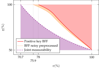
Figure 4: Regions where the key rate becomes zero as a function of visibility and detection efficiency. The region where the BFF 3 outcome protocol with partially entangled states is secure is above the red line, the case where we include also noisy preprocessing is above the orange dotted line, while the purple line denotes the boundary below which Bob’s observables are jointly measurable, rendering any protocol insecure in that region.

We will now study the robustness of our technique in the presence of depolarizing noise acting on the initial state together with photon losses. The reference statistics are obtained by adding depolarizing noise to the state generated by the source as

$$\rho=v|\psi(\theta)\rangle\!\langle\psi(\theta)|+\frac{1-v}{4}\mathbbm{1},$$ (12)

where $v$ is denoted as visibility. We show in Fig. 4 the region in the space of parameters $\eta$ and $v$ where the key rate is positive. This analysis is conducted in two scenarios. One where we optimize the key rate only over the angle of the partially entangled state and another where we additionally perform optimal noisy pre-processing. The key rate was computed using BFF with full statistics and keeping Bob’s undetected photons as a separate outcome. We noticed that for visibilities smaller than one, the use of partially entangled states (and of noisy pre-processing) leads to an improvement also for the BFF case where the three outcomes of Bob are kept separate. Moreover, we include in the plot a curve from [41] which displays the zone where the evolution of $X$ and $Z$ measurements of Bob under depolarizing noise and losses are jointly measurable. When Bob’s measurements are jointly measurable, the correlations between Alice and Bob are unsteerable. As a result, no secure key can be extracted in this region regardless of the initial state prepared, and regardless of the measurements performed by the semi-trusted party. One can see in Fig. 4 that, for non-unit values of the visibility, a region exists wherein the key rate is non-positive, and the noisy versions of $X$ and $Z$ observables are not jointly measurable. This suggests that refining our protocol or improving its analysis might enhance its resilience against such noise. Specifically, exploring variations of our protocol involving secret key extraction from both Alice’s measurements and using the BFF technique with higher levels of the NPA hierarchy may prove insightful. However, recall that the joint measurability of Bob’s measurements is only a necessary condition for the protocol to be insecure. For non-unit values of visibility, stricter conditions may be necessary.

Theoretical distance estimate of implementability.— Finally, in order to estimate the distance at which our protocols can be implemented, we will deploy a model where Alice’s and Bob’s devices observe dark counts. We describe our model in appendix D. It is crucial to note that the noise model we are about to use is regarded as part of the untrusted quantum channel that evolves the untrusted state $\rho$. Therefore, as it is typically assumed in standard QKD protocols, dark counts are not included in the model of Alice’s semi-trusted device, ensuring that her measurements remain anti-commuting. For convenience, we will evolve Alice’s ideal POVMs to compute the probability distribution resulting from our model as this is equivalent to evolving the state $\rho$.

Figure 5: Plot of the key rate as a function of the distance in a model that includes photon losses, depolarizing noise, and dark counts in the case where we assume that Alice’s measurements anti-commute.

We draw inspiration for our model from a framework detailed in [33], which provides a comprehensive depiction of the behavior observed in their experimental setup. Dark counts are essentially random clicks generated by detectors resulting from thermal fluctuations inside the detectors. These are of critical importance particularly when operating at low detection efficiencies, as their frequency becomes noteworthy over the fraction of rounds that have not been discarded under the fair sampling assumption.

Let us provide Bob’s measurement operators. We choose to categorize all the events where Bob experiences zero or double clicks as a separate outcome $\varnothing$. As explained in appendix D, his POVMs evolve as

$$N_{1,2|y}(\eta_{B},p_{d}) =\eta_{B}(1-p_{d})N_{1,2|y}+(1-\eta_{B})p_{d}(1-p_{d})\mathbbm{1},$$ (13)

$$N_{\varnothing|y}(\eta_{B},p_{d}) =\big{(}p_{d}\eta_{B}+(1-\eta_{B})(p_{d}^{2}+(1-p_{d})^{2})\big{)}\mathbbm{1},$$ (14)

where $N_{b|y}$ are the projective measurements that Bob performs in the ideal case.

On Alice’s side, we choose to discard all events where her detectors do not click or where they both click. As we discard these events, we will need to renormalize her POVMs dividing them by the probability of having only one click. We show in appendix D that the measurement operators of Alice $M_{1|x}(\eta_{A},p)$ can be expressed in terms of the ideal ones $M_{1|x}$ as

$$M_{1|x}(\eta_{A},p_{d})=\frac{\eta_{A}(1-p_{d})M_{1|x}+(1-\eta_{A})p_{d}(1-p_{d})\mathbbm{1}}{1-p_{d}\eta_{A}-(1-\eta_{A})(p_{d}^{2}+(1-p_{d})^{2})},$$ (15)

and $M_{2|x}(\eta_{A},p_{d})=\mathbbm{1}-M_{1|x}(\eta_{A},p_{d})$.

Figure 6: Plot of the key rate as a function of the distance in a model that includes photon losses, depolarizing noise, and dark counts in the case where we do not assume that Alice’s measurements anti-commute.

For the reference statistics, we will take into account the values of visibility and dark counts of the most advanced experiment we are aware of, which employs an entanglement-based scheme [33]. Specifically, we take $v=0.99$ and $p_{d}=10^{-6}$. As far as the detection efficiency is concerned, we will take into account a fixed component $\eta_{\text{fix}}$ due to the efficiency of the detectors and of the other optical components, and a variable component that accounts for optical fiber losses based on its length $l$, given by $\eta_{\text{fiber}}=10^{-\alpha\cdot l/10}$. Here, we will use the typical value for telecom wavelength of $\alpha=0.2\,dB/km$ (see e.g. [38, 32]). Since the source is placed very close to Bob’s laboratory, we can ignore the losses arising due to the fiber. Consequently, his efficiency will be $\eta_{B}=\eta_{\text{fix}}$, while Alice’s one is $\eta_{A}(l)=\eta_{\text{fix}}\cdot 10^{-\alpha\cdot l/10}$. Given these parameters of the setup, in Fig. 5 we plot the lower bound to the asymptotic key rate as a function of the distance. To show the number of key bits generated in each actual round of the protocol (and not only in the ones that have been retained), the key rates in Fig. 5 have been multiplied by the probability of retaining a round which is $1-p_{d}\eta_{A}-(1-\eta_{A})(p_{d}^{2}+(1-p_{d})^{2})$. To compute the key rates, we used the BFF method where Bob’s third outcomes are kept separate. We provide the plot for different values of $\eta_{\text{fix}}$. For each specific $\eta_{\text{fix}}$ and $l$ value, we optimized the key rate by adjusting the angle of the partially entangled state and the amount of noisy pre-processing. Let us remark that the optimization for each value of $l$ resulted only in a few kilometers of improvement compared to the case where we optimize only for $l=0$ and apply the same parameters for each $l$. This is due to the fact that the key rate drops quickly to zero when $\eta_{A}$ and $p_{d}$ reach a similar order of magnitude.

Finally, we include in Fig. 6 a plot where we estimate the achievable distance in the case of a protocol where we do not assume that Alice’s observables anti-commute and Bob makes three measurements as explained before. Similarly to the previous case, we computed the key rates using the BFF method where Bob’s third outcomes are kept separate, and we fixed $v=0.99$ and $p_{d}=10^{-6}$. In this case, for each specific $\eta_{\text{fix}}$ value, we optimized the key rate by adjusting the parameters $\theta$, $\alpha_{1}$, $\alpha_{2}$, $\beta_{1}$, $\beta_{2}$, $\beta_{3}$, $q$ for a distance of $l=0$, and then applied the same parameters to compute the key rate across all other distances. This was due to the fact that computing a key rate in this setting requires a higher level of the NPA hierarchy and optimizing over the parameters in question for each value of $l$ would require a too large computational time. We can see that we can obtain similar distances as in the previous case, but Bob’s device needs greater detection efficiencies. In particular, for $\eta_{\text{fix}}\lesssim 70\%$ this type of protocol is not secure, while the one where we assume that Alice’s observables anticommute can still be proven secure. This requirement can be inconvenient in a client-server scenario where Bob is a user with limited resources.

Discussion.— We applied to a 1SDI scenario the most recent methods to derive lower bounds on the conditional Von Neumann entropy. We provided lower bounds with both analytical and numerical methods and showed that our analytical results can be recovered with the numerical method of [44]. We showed that the first QKD protocol ever introduced, the BB84 protocol, can be proven secure in an entanglement-based 1SDI scenario with up to 50.1% detection efficiency on the untrusted side. This result is almost optimal as no protocol employing two untrusted measurements can achieve security below a 50% detection efficiency threshold. Furthermore, we observed that, by increasing the number of Gauss-Radau coefficients, we can get closer to this critical threshold.

Detection efficiencies above 50% have now been obtained in a large number of photonic experiments both in the context of Bell tests [49, 50, 51], Quantum Random Number Generation [52, 53, 54, 55, 56, 57, 58, 59] and DI QKD [33]. Therefore, our protocol is well within the current experimental limits. It is worth noting that DI QKD protocols can also be proven secure at similar distances as the ones simulated in this article but they require more complex schemes [36, 38] and much higher detection efficiencies. In the case of [38], for example, the detection efficiency required to prove security with unit visibility is $96.1\%$. Notice also that [38] assumes a dark count rate of $10^{-7}$, while here we make the more pessimistic assumption of a dark count rate of $10^{-6}$.

Finally, while our findings achieve near-optimal thresholds in terms of detection efficiency, it remains an open question whether our result is optimal also in terms of depolarizing noise. As we showed in Fig. 4, there is a region where either our protocol could be improved, or there is an attack that goes beyond the joint measurability of Bob’s measurements. Let us also point out that our work can be easily extended to the case where the measurements of Alice are not perfectly anticommuting using the BFF method. For instance, one can explore the case of $A_{1}A_{2}+A_{2}A_{1}=\epsilon\mathbbm{1}$, where $\epsilon$ is small. Another possible extension is to consider multipartite scenarios like Conference Key Agreement.

The code used to compute the key rates numerically can be found in the GitHub folder [60].

Acknowledgnements.— We extend our gratitude to Stefano Pironio for his extensive discussions and valuable insights regarding our work. His contributions have been fundamental in enhancing the quality and depth of our research. We thank Thomas Van Himbeeck for discussions on the possibility of extending the security of our work to the finite-size case. We thank Erik Woodhead for developing an open-source Julia library to compute NPA relaxations, and Abhishek Mishra for his work in extending it. We thank Marco Avesani for the discussions on estimating the distance of implementability of our work. We acknowledge funding from the VERIqTAS project within the QuantERA II Programme that has received funding from the European Union’s Horizon 2020 research and innovation programme under Grant Agreement No 101017733 and the F.R.S-FNRS Pint-Multi programme under Grant Agreement R.8014.21, from the European Union’s Horizon Europe research and innovation programme under the project "Quantum Security Networks Partnership" (QSNP, grant agreement No 101114043), from the F.R.S-FNRS through the PDR T.0171.22, from the FWO and F.R.S.-FNRS under the Excellence of Science (EOS) programme project 40007526, from the FWO through the BeQuNet SBO project S008323N, from the Belgian Federal Science Policy through the contract RT/22/BE-QCI and the EU “BE-QCI" programme. Funded by the European Union. Views and opinions expressed are however those of the authors only and do not necessarily reflect those of the European Union, which cannot be held responsible for them.

Appendix A Brown-Fawzi-Fawzi bounds

In this appendix, we provide the non-commutative polynomial optimization problem that we used to lower bound the conditional Von Neumann entropy to verify the security of our protocols. Our lower bound is a simple extension of the work of [44] to a steering scenario.

Let $t_{1},\dots,t_{m}$ and $w_{1},\dots,w_{m}$ be the nodes and weights of an $m$-point Gauss-Radau quadrature on $(0,1]$ where we fix $t_{m}=1$. These coefficients can be computed efficiently in terms of Legendre polynomials [61]. Moreover, let

$$\alpha_{i}=\frac{3}{2}\min\left\{\frac{1}{t_{i}},\frac{1}{1-t_{i}}\right\}.$$ (16)

We have that

$$H(A_{1}|E)\geq\sum_{i=1}^{m-1}\frac{w_{i}}{t_{i}\ln(2)}+\sum_{i=1}^{m-1}\frac{w_{i}}{t_{i}\ln(2)}O_{i},$$ (17)

where $O_{i}$ are the solutions to the following polynomial optimization problems

inf $$\sum_{a}\langle\psi|M_{a|1}(Z_{a,i}+Z^{*}_{a,i}+(1-t_{i})Z_{a,i}^{*}Z_{a,i})+t_{i}Z_{a,i}Z^{*}_{a,i}|\psi\rangle$$ (18)

s.t. $$\langle\psi|M_{a|x}N_{b|y}|\psi\rangle=p(a,b|x,y),$$ (19)

$$\sum_{a}M_{a|x}=\sum_{a}N_{b|y}=\mathbbm{1},$$ (20)

$$M_{a|x}\geq 0,\quad N_{b|y}\geq 0,$$ (21)

$$Z_{a,i}^{*}Z_{a,i}\leq\alpha_{i},\quad Z_{a,i}Z^{*}_{a,i}\leq\alpha_{i},$$ (22)

$$[M_{a|x},N_{b|y}]=[M_{a|x},Z^{(*)}_{a,i}]=[Z_{a,i}^{(*)},N_{b|y}]=0,$$ (23)

$$(M_{1|1}-M_{2|1})(M_{1|2}-M_{2|2})+(M_{1|2}-M_{2|2})(M_{1|1}-M_{2|1})=0.$$ (24)

In the last constraint (eq. (24)) of the optimization problem, we introduced the anti-commutation constraint. Note that we expressed w.l.o.g. $A_{x}=M_{1|x}-M_{2|x}$. The probabilities $p(a,b|x,y)$ are the ones observed during the experiment or, in our case, computed from the simulations.

In the case where we perform noisy preprocessing, the measurement operators $M_{a|1}$ in the objective function need to be replaced with

$$M_{1|1} \rightarrow(1-q)M_{1|1}+qM_{2|1},$$ (25)

$$M_{2|1} \rightarrow(1-q)M_{2|1}+qM_{1|1}.$$ (26)

The latter problem is a non-commutative polynomial optimization problem and it can be relaxed to a hierarchy of semi-definite programs [46]. The lower bound that we obtain from the solution of this problem is increasingly tighter as a function of the level of the hierarchy and as a function of the number of points of the Gauss-Radau quadrature. For the computations performed in this work in the case where Alice’s observables are assumed to anti-commute, we kept the level of the localizing matrices of the NPA hierarchy fixed to $1$ and used $m=15$ in the Gauss Radau quadrature. The level of the principal moment matrix was slightly bigger than one in order to make sure that all the terms that appear in the localizing moment matrices were also present in the principal one. Additionally, our analysis revealed that for the problems examined in this article, incorporating localizing matrices representing the constraints $Z_{a,i}^{*}Z_{a,i}\leq\alpha_{i}$ and $Z_{a,i}Z^{*}_{a,i}\leq\alpha_{i}$ did not improve the lower bounds on the conditional Von Neumann entropy. Consequently, we opted for simpler constraints $\langle\psi|Z_{a,i}^{*}Z_{a,i}|\psi\rangle\leq\alpha_{i}$ and $\langle\psi|Z_{a,i}Z^{*}_{a,i}|\psi\rangle\leq\alpha_{i}$, which still establish a valid lower bound on the conditional Von Neumann entropy.

Finally, in the case where we analyzed a DI protocol with a fair sampling assumption on Alice’s side, we did not include any localizing matrix. This comes from two reasons. First, we did not need to enforce anti-commutativity and, second, as before, we used the simpler constraints $\langle\psi|Z_{a,i}^{*}Z_{a,i}|\psi\rangle\leq\alpha_{i}$ and $\langle\psi|Z_{a,i}Z^{*}_{a,i}|\psi\rangle\leq\alpha_{i}$. However, in this scenario, achieving satisfactory results required the use of a principal moment matrix at level $2+ABZ$.

Appendix B Analytical bounds

In this appendix, we will prove extensively the analytical lower bound on the key rate described in the main text.

We will bound the quantity $H(A_{1}|E)$ as a function of input-output statistics derived from measurements of $A_{1,2}$ and $B_{1,2}$ that only have two possible outcomes. In this way, we can use Jordan’s lemma [45] and reduce our problem to deriving a convex lower bound on the conditional Von Neumann entropy between Alice and Eve in the case where Alice and Bob’s systems are two-dimensional.

If the secret key is extracted from the outcomes of the measurement of the two-outcomes observable $A_{1}$ on Alice’s side, the conditional Von Neumann entropy of Alice conditioned on Eve can be bounded by [42]

$$H(A_{1}|E)\geq 1-\phi\left(\langle|\bar{A}_{1}\otimes B\rangle|\right),$$ (27)

where $B$ is any unitary observable on Bob’s subspace, $\bar{A}_{1}$ is an observable on Alice’s subspace that anticommutes with $A_{1}$, and $\phi(x)=h(1/2(1+x))$ where $h(x)$ is the binary entropy function. Under the same assumptions, a second bound that we can use [43] is

$$H(A_{1}|E)\geq\phi\left(\langle A_{1}\rangle\right)\\ -\phi\left(\sqrt{\langle A_{1}\rangle^{2}+\langle\bar{A}_{1}\otimes B\rangle^{2}}\right),$$ (28)

At this point, we need to find a lower bound on $\langle\bar{A}_{1}\otimes B\rangle$ as a function of the input-output statistics of Alice and Bob’s devices such that it is independent of what is the form of the measurements performed by Bob.

For the steering scenario, we can choose to bound the correlator directly. By assuming that $\bar{A}_{1}=A_{2}$, and choosing $B=B_{2}$, we can evaluate $\langle A_{2}\otimes B_{2}\rangle$ from the input-output statistics. In this case, using eq. (28), our bound becomes of the type

$$H(A_{1}|E)\geq\phi\left(\langle A_{1}\rangle\right)-\phi\left(\sqrt{\langle A_{1}\rangle^{2}+\langle A_{2}\otimes B_{2}\rangle^{2}}\right).$$ (29)

Notice that for the case of eq. (27) applied to an honest implementation where Alice and Bob measure Pauli operators $Z,X$ on a maximally entangled state undergoing losses and depolarizing noise, we obtain the same lower bound of [19] just by assuming the anti-commutativity of Alice’s measurements and making a fair sampling assumption on her side.

Finally, in order to use Jordan’s lemma, we will need to prove that the bounds obtained are convex in the variables $x=\langle A_{2}\otimes B_{2}\rangle$ and $z=\langle A_{1}\rangle$.

The case of eq. (27) is straightforward since the binary entropy function is a concave function. Let us now prove the convexity for the case of eq. (28).

We start with the direct case. We need to show that, for the function

$$f(z,x)=\phi(z)-\phi\left(\sqrt{z^{2}+x^{2}}\right),$$ (30)

the hessian matrix is such that

$$\mathbf{H}(f(z,x))=\begin{pmatrix}&\frac{d^{2}}{dz^{2}}f(z,x)&\frac{d^{2}}{sz\,dx}f(z,x)\\ \\ &\frac{d^{2}}{sz\,dx}f(z,x)&\frac{d^{2}}{dx^{2}}f(z,x)\end{pmatrix}\geq 0.$$ (31)

Being a $2\times 2$ matrix, the positivity is ensured by the positivity of the diagonal elements and of the determinant. We have

$$\frac{d^{2}}{dz^{2}}f(z,x)=\frac{x^{2}}{\ln(2)}\left(\frac{x^{2}-1+2z^{2}}{(z^{2}+x^{2})(1-x^{2}-z^{2})(1-z^{2})}+\frac{\text{arctanh}\!\left(\sqrt{z^{2}+x^{2}}\right)}{\left(x^{2}+z^{2}\right)^{3/2}}\right).$$ (32)

we can easily notice that, since $z^{2}\leq 1$, the positivity of eq. (32) is ensured by the condition $z^{2}+x^{2}\leq 1$ which is proven in appendix C.

The second diagonal element is

$$\frac{d^{2}}{dx^{2}}f(z,x)=\frac{1}{\ln(2)}\left(\frac{x^{2}}{(z^{2}+x^{2})(1-x^{2}-z^{2})}+z^{2}\frac{\text{arctanh}\!\left(\sqrt{z^{2}+x^{2}}\right)}{\left(x^{2}+z^{2}\right)^{3/2}}\right),$$ (33)

whose positivity is ensured by the same conditions as before. Finally, the determinant is

$$\frac{d^{2}}{dz^{2}}f(z,x)\frac{d^{2}}{dx^{2}}f(z,x)-\left(\frac{d^{2}}{dx\,dz}f(z,x)\right)^{2}=\\ \frac{x^{2}}{(\ln(2))^{2}(z^{2}+x^{2})^{2}(1-x^{2}-z^{2})(1-z^{2})}\bigg{(}\sqrt{z^{2}+x^{2}}\,\text{arctanh}\,\sqrt{z^{2}+x^{2}}-(z^{2}+x^{2})\bigg{)},$$ (34)

whose positivity is ensured by $z^{2}\leq 1$, by $z^{2}+x^{2}\leq 1$, and by $\text{arctanh}(x)\geq x$.

We conclude that eq. (29) is a valid lower bound under the assumptions of anti-commutativity between $A_{1}$ and $A_{2}$ and under a fair sampling assumption on Alice’s side. Notice that Alice’s Hilbert space dimension does not need to be bounded.

Appendix C Domain of the correlations

In this appendix, we prove the condition

$$\langle A\rangle^{2}+\langle\bar{A}\otimes B\rangle^{2}\leq 1,$$ (35)

which is required in appendix B.

Let us begin by considering a state $\rho_{AB}$ and then purifying it to $|\psi_{ABE}\rangle$ such that $\rho_{AB}=\mathrm{Tr}_{E}\ \psi_{ABE}$ where $E$ denotes the ancillary system. Now, any general state $|\psi_{ABE}\rangle\in\mathbbm{C}^{2}\otimes\mathcal{H}_{BE}$ can be written as

$$|\psi_{ABE}\rangle=\sum_{i=0,1}\lambda_{i}|i\rangle_{A}|e_{i}\rangle_{BE}$$ (36)

where $\lambda_{i}\geq 0$, $\sum_{i=0,1}\lambda_{i}^{2}=1$ and $|e_{i}\rangle_{BE}$ are normalised but in general not orthogonal. Now, evaluating the left-hand side of eq. (35) by plugging in the state (36), we obtain

$$\langle Z\rangle^{2}+\langle X\otimes B\rangle^{2}=\left(\lambda_{0}^{2}-\lambda_{1}^{2}\right)^{2}+4\lambda_{0}^{2}\lambda_{1}^{2}\ \left(\mathrm{Re}\langle e_{0}|B|e_{1}\rangle\right)^{2}$$ (37)

where we used the fact that $B$ is Hermitian. As $B$ is unitary, we have that $-1\leq\mathrm{Re}\langle e_{0}|B|e_{1}\rangle\leq 1$ using which we arrive at

$$\langle Z\rangle^{2}+\langle X\otimes B\rangle^{2}\leq\left(\lambda_{0}^{2}-\lambda_{1}^{2}\right)^{2}+4\lambda_{0}^{2}\lambda_{1}^{2}=\left(\lambda_{0}^{2}+\lambda_{1}^{2}\right)^{2}=1.$$ (38)

This completes the proof.

Appendix D A model for dark counts and losses

In this appendix, we present a model for computing the measurement operators of Alice and Bob, taking into account photon loss and dark counts.

Figure 7: Schematic representation of an ideal detector in the absence of losses and dark counts. A polarizing beam splitter divides the incoming photonic state into two paths. At the two output ports of the beam splitter, we place two detectors and each of them corresponds to one of the two possible outcomes. Outcomes "1" and "2" correspond to two orthogonal polarizations of the photon.

In Fig. 7, we represent an ideal detector. Let us initially address photon loss. When a photon arrives at the measurement device (with probability $\eta$), it encounters a polarizing beam splitter, which then directs it to one of two detectors based on its polarization state. If the photon is lost (with probability $1-\eta$), then neither detector clicks.

Let us now assume that the detectors of Alice and Bob exhibit also a dark count behavior, with each of the two possible outcomes having a probability of $p_{d}$ of registering a spurious click in every round of the protocol. Our setup does not allow us to differentiate whether the detection was due to a genuine photon detection, or a dark count.

Let us delineate the four possible detection outcomes.

1. Single click in the first detector: This outcome indicates that only the detector "1" clicked. It could arise from the detection of a photon with a specific polarization or a dark count in the first detector.

2. Single click in the second detector: This outcome indicates that only the detector "2" clicked.

3. Double click: It occurs when both detectors register a click simultaneously. This can arise from both detectors experiencing dark counts, or one detecting a photon while the other registers a dark count.

4. No click: When neither detector registers a click, suggesting the photon was lost and no dark counts occurred.

Let us now evaluate the POVMs related to each of these four events. We will take into account the ideal POVMs $M_{1}$ and $M_{2}$ of the photon being detected by the first and second detectors, respectively, the efficiency $\eta$ of the photon’s arrival at the detectors, and the probability $p_{d}$ of a dark count occurring in each detector.

Assuming the photon arrives at the measurement device, four possible events can occur. We list them in table 1.

Event	POVM	Outcome Type
Photon at first detector, no dark count at second	$\eta\times(1-p_{d})\times M_{1}$	Single click in the first
Photon at second detector, no dark count at first	$\eta\times(1-p_{d})\times M_{2}$	Single click in the second
Photon at first detector, dark count at second	$\eta\times p_{d}\times M_{1}$	Double click
Photon at second detector, dark count at first	$\eta\times p_{d}\times M_{2}$	Double click

Table 1: POVMs of detection events with photon arrival, considering dark counts and categorized by outcome type.

For the scenario where the photon does not arrive, we have four cases which we list in table 2.

Event	POVM	Outcome Type
No dark count in either detector	$(1-\eta)\times(1-p_{d})^{2}\times\mathbbm{1}$	No click
Dark count in the first detector only	$(1-\eta)\times p_{d}\times(1-p_{d})\times\mathbbm{1}$	Single click in the first
Dark count in the second detector only	$(1-\eta)\times(1-p_{d})\times p_{d}\times\mathbbm{1}$	Single click in the second
Dark counts in both detectors	$(1-\eta)\times p_{d}^{2}\times\mathbbm{1}$	Double click

Table 2: POVMs of detection events without photon arrival, categorized by outcome type.

To compute the measurement operators of Bob, given the ideal measurement operators $N_{1|x}$ for outcome 1 and $N_{2|x}$ for outcome 2, we need to consider the probabilities of each event as previously discussed. We obtain in this way four measurement operators $N_{b|y}(\eta_{B},p_{d})$ corresponding to the four outcome types, where $\eta_{B}$ is the detection efficiency at Bob’s side.

$$N_{1|y}(\eta_{B},p_{d}) =\eta_{B}(1-p_{d})N_{1|y}+(1-\eta_{B})p_{d}(1-p_{d})\mathbbm{1},$$ (39)

$$N_{2|y}(\eta_{B},p_{d}) =\eta_{B}(1-p_{d})N_{2|y}+(1-\eta_{B})p_{d}(1-p_{d})\mathbbm{1},$$ (40)

$$N_{\text{Dc}|y}(\eta_{B},p_{d}) =\big{(}p_{d}\eta_{B}+(1-\eta_{B})p_{d}^{2}\big{)}\mathbbm{1},$$ (41)

$$N_{\text{Nc}|y}(\eta_{B},p_{d}) =(1-\eta_{B})(1-p_{d})^{2}\mathbbm{1}.$$ (42)

For simplicity, we will group Bob’s no clicks and double clicks into a single outcome, obtaining in this way

$$N_{\varnothing|y}(\eta_{B},p_{d})=\big{(}p_{d}\eta_{B}+(1-\eta_{B})(p_{d}^{2}+(1-p_{d})^{2})\big{)}\mathbbm{1}.$$ (43)

Let us finally focus on Alice’s measurements. Her ideal POVMs are denoted as $M_{a|x}$. Given the assumption that the probability of a click in Alice’s detector is independent of the basis choice, we are allowed to discard events where both her detectors do not click or where they both click. As we discard these events, we will need to renormalize Alice’s POVMs dividing them by the probability of having only one click. Consequently, the measurement operators of Alice $M_{a|x}(\eta_{A},p)$ can be expressed in terms of the ideal ones $M_{1|x}$ as

$$M_{1|x}(\eta_{A},p_{d})=\frac{\eta_{A}(1-p_{d})M_{1|x}+(1-\eta_{A})p_{d}(1-p_{d})\mathbbm{1}}{1-p_{d}\eta_{A}-(1-\eta_{A})(p_{d}^{2}+(1-p_{d})^{2})},$$ (44)

and $M_{2|x}(\eta_{A},p_{d})=\mathbbm{1}-M_{1|x}(\eta_{A},p_{d})$. Here, $\eta_{A}$ is the detection efficiency on Alice’s side.

References

- Scarani et al. [2009] V. Scarani, H. Bechmann-Pasquinucci, N. J. Cerf, M. Dušek, N. Lütkenhaus, and M. Peev, The security of practical quantum key distribution, Rev. Mod. Phys. 81, 1301 (2009).
- Xu et al. [2020] F. Xu, X. Ma, Q. Zhang, H.-K. Lo, and J.-W. Pan, Secure quantum key distribution with realistic devices, Rev. Mod. Phys. 92, 025002 (2020).
- Lydersen et al. [2010] L. Lydersen, C. Wiechers, C. Wittmann, D. Elser, J. Skaar, and V. Makarov, Hacking commercial quantum cryptography systems by tailored bright illumination, Nature Photonics 4, 686 (2010).
- Gerhardt et al. [2011] I. Gerhardt, Q. Liu, A. Lamas-Linares, J. Skaar, C. Kurtsiefer, and V. Makarov, Full-field implementation of a perfect eavesdropper on a quantum cryptography system, Nat. Commun. 2, 1 (2011).
- Jain et al. [2011] N. Jain, C. Wittmann, L. Lydersen, C. Wiechers, D. Elser, C. Marquardt, V. Makarov, and G. Leuchs, Device calibration impacts security of quantum key distribution, Phys. Rev. Lett. 107, 110501 (2011).
- Bugge et al. [2014] A. N. Bugge, S. Sauge, A. M. M. Ghazali, J. Skaar, L. Lydersen, and V. Makarov, Laser damage helps the eavesdropper in quantum cryptography, Phys. Rev. Lett. 112, 070503 (2014).
- Acín et al. [2007] A. Acín, N. Brunner, N. Gisin, S. Massar, S. Pironio, and V. Scarani, Device-independent security of quantum cryptography against collective attacks, Phys. Rev. Lett. 98, 230501 (2007).
- Primaatmaja et al. [2023] I. W. Primaatmaja, K. T. Goh, E. Y.-Z. Tan, J. T.-F. Khoo, S. Ghorai, and C. C.-W. Lim, Security of device-independent quantum key distribution protocols: a review, Quantum 7, 932 (2023).
- Lo et al. [2012] H.-K. Lo, M. Curty, and B. Qi, Measurement-device-independent quantum key distribution, Phys. Rev. Lett. 108, 130503 (2012).
- Braunstein and Pirandola [2012] S. L. Braunstein and S. Pirandola, Side-channel-free quantum key distribution, Phys. Rev. Lett. 108, 130502 (2012).
- Pawłowski and Brunner [2011] M. Pawłowski and N. Brunner, Semi-device-independent security of one-way quantum key distribution, Phys. Rev. A 84, 010302 (2011).
- Woodhead and Pironio [2015] E. Woodhead and S. Pironio, Secrecy in prepare-and-measure clauser-horne-shimony-holt tests with a qubit bound, Phys. Rev. Lett. 115, 150501 (2015).
- Woodhead [2016] E. Woodhead, Semi device independence of the bb84 protocol, New J. Phys. 18, 055010 (2016).
- Yin et al. [2014] Z.-Q. Yin, C.-H. F. Fung, X. Ma, C.-M. Zhang, H.-W. Li, W. Chen, S. Wang, G.-C. Guo, and Z.-F. Han, Mismatched-basis statistics enable quantum key distribution with uncharacterized qubit sources, Phys. Rev. A 90, 052319 (2014).
- Ioannou et al. [2022a] M. Ioannou, M. A. Pereira, D. Rusca, F. Grünenfelder, A. Boaron, M. Perrenoud, A. A. Abbott, P. Sekatski, J.-D. Bancal, N. Maring, et al., Receiver-device-independent quantum key distribution, Quantum 6, 718 (2022a).
- Ioannou et al. [2022b] M. Ioannou, P. Sekatski, A. A. Abbott, D. Rosset, J.-D. Bancal, and N. Brunner, Receiver-device-independent quantum key distribution protocols, New J. Phys. 24, 063006 (2022b).
- Mayers [2001] D. Mayers, Unconditional security in quantum cryptography, Journal of the ACM (JACM) 48, 351 (2001).
- Tomamichel and Renner [2011] M. Tomamichel and R. Renner, Uncertainty relation for smooth entropies, Phys. Rev. Lett. 106, 110506 (2011).
- Branciard et al. [2012] C. Branciard, E. G. Cavalcanti, S. P. Walborn, V. Scarani, and H. M. Wiseman, One-sided device-independent quantum key distribution: Security, feasibility, and the connection with steering, Phys. Rev. A 85, 010301 (2012).
- Lucamarini et al. [2012] M. Lucamarini, G. Vallone, I. Gianani, P. Mataloni, and G. Di Giuseppe, Device-independent entanglement-based bennett 1992 protocol, Phys. Rev. A 86, 032325 (2012).
- Tomamichel et al. [2013] M. Tomamichel, S. Fehr, J. Kaniewski, and S. Wehner, A monogamy-of-entanglement game with applications to device-independent quantum cryptography, New Journal of Physics 15, 103002 (2013).
- Vallone et al. [2014] G. Vallone, A. Dall´Arche, M. Tomasin, and P. Villoresi, Loss tolerant device-independent quantum key distribution: a proof of principle, New J. Phys. 16, 063064 (2014).
- Gehring et al. [2015] T. Gehring, V. Händchen, J. Duhme, F. Furrer, T. Franz, C. Pacher, R. F. Werner, and R. Schnabel, Implementation of continuous-variable quantum key distribution with composable and one-sided-device-independent security against coherent attacks, Nat. Commun. 6, 8795 (2015).
- Xin et al. [2020] J. Xin, X.-M. Lu, X. Li, and G. Li, One-sided device-independent quantum key distribution for two independent parties, Opt. Express 28, 11439 (2020).
- Wiseman et al. [2007] H. M. Wiseman, S. J. Jones, and A. C. Doherty, Steering, entanglement, nonlocality, and the Einstein-Podolsky-Rosen paradox, Phys. Rev. Lett. 98, 140402 (2007).
- Arnon-Friedman et al. [2018] R. Arnon-Friedman, F. Dupuis, O. Fawzi, R. Renner, and T. Vidick, Practical device-independent quantum cryptography via entropy accumulation, Nat. Commun. 9, 459 (2018).
- Dupuis et al. [2020] F. Dupuis, O. Fawzi, and R. Renner, Entropy accumulation, Commun. in Math. Phys. 379, 867 (2020).
- Metger et al. [2022] T. Metger, O. Fawzi, D. Sutter, and R. Renner, Generalised entropy accumulation, in 2022 IEEE 63rd An. Symp. on FOCS (IEEE, 2022) pp. 844–850.
- de la Torre et al. [2016] G. de la Torre, J.-D. Bancal, S. Pironio, V. Scarani, et al., Randomness in post-selected events, New J. Phys. 18, 035007 (2016).
- Sandfuchs and Wolf [2023] M. Sandfuchs and R. Wolf, Coherent attacks are stronger than collective attacks on diqkd with random postselection, arXiv preprint arXiv:2306.07364 (2023).
- Bennett and Brassard [2014] C. H. Bennett and G. Brassard, Quantum cryptography: Public key distribution and coin tossing, Theoretical Computer Science 560, 7 (2014), theoretical Aspects of Quantum Cryptography – celebrating 30 years of BB84.
- Acín et al. [2016] A. Acín, D. Cavalcanti, E. Passaro, S. Pironio, and P. Skrzypczyk, Necessary detection efficiencies for secure quantum key distribution and bound randomness, Phys. Rev. A 93, 012319 (2016).
- Liu et al. [2022] W.-Z. Liu, Y.-Z. Zhang, Y.-Z. Zhen, M.-H. Li, Y. Liu, J. Fan, F. Xu, Q. Zhang, and J.-W. Pan, Toward a photonic demonstration of device-independent quantum key distribution, Phys. Rev. Lett. 129, 050502 (2022).
- Orsucci et al. [2020] D. Orsucci, J.-D. Bancal, N. Sangouard, and P. Sekatski, How post-selection affects device-independent claims under the fair sampling assumption, Quantum 4, 238 (2020).
- Vallone [2013] G. Vallone, Einstein-podolsky-rosen steering: Closing the detection loophole with non-maximally-entangled states and arbitrary low efficiency, Phys. Rev. A 87, 020101 (2013).
- Gisin et al. [2010] N. Gisin, S. Pironio, and N. Sangouard, Proposal for implementing device-independent quantum key distribution based on a heralded qubit amplifier, Phys. Rev. Lett. 105, 070501 (2010).
- Wollmann et al. [2016] S. Wollmann, N. Walk, A. J. Bennet, H. M. Wiseman, and G. J. Pryde, Observation of genuine one-way einstein-podolsky-rosen steering, Phys. Rev. Lett. 116, 160403 (2016).
- Zapatero and Curty [2019] V. Zapatero and M. Curty, Long-distance device-independent quantum key distribution, Scientific Reports 9, 17749 (2019).
- Devetak and Winter [2005] I. Devetak and A. Winter, Distillation of secret key and entanglement from quantum states, Proc. R. Soc. A 461, 207 (2005).
- Renner et al. [2005] R. Renner, N. Gisin, and B. Kraus, Information-theoretic security proof for quantum-key-distribution protocols, Phys. Rev. A 72, 012332 (2005).
- Masini et al. [2024] M. Masini, M. Ioannou, N. Brunner, S. Pironio, and P. Sekatski, Article in preparation, (2024).
- Woodhead et al. [2021] E. Woodhead, A. Acín, and S. Pironio, Device-independent quantum key distribution with asymmetric CHSH inequalities, Quantum 5, 443 (2021).
- Masini et al. [2022] M. Masini, S. Pironio, and E. Woodhead, Simple and practical DIQKD security analysis via BB84-type uncertainty relations and Pauli correlation constraints, Quantum 6, 843 (2022).
- Brown et al. [2021] P. Brown, H. Fawzi, and O. Fawzi, Device-independent lower bounds on the conditional von neumann entropy, arXiv preprint arXiv:2106.13692 (2021).
- Jordan [1875] C. Jordan, Essai sur la géométrie à dimensions, Bull. Soc. Math. Fr. 3, 103 (1875).
- Navascués et al. [2008] M. Navascués, S. Pironio, and A. Acín, A convergent hierarchy of semidefinite programs characterizing the set of quantum correlations, New J. Phys. 10, 073013 (2008).
- Pironio et al. [2010] S. Pironio, M. Navascués, and A. Acín, Convergent relaxations of polynomial optimization problems with noncommuting variables, SIAM Journal on Optimization 20, 2157 (2010), https://doi.org/10.1137/090760155 .
- Ho et al. [2020] M. Ho, P. Sekatski, E. Y.-Z. Tan, R. Renner, J.-D. Bancal, and N. Sangouard, Noisy preprocessing facilitates a photonic realization of device-independent quantum key distribution, Phys. Rev. Lett. 124, 230502 (2020).
- Shalm et al. [2015] L. K. Shalm, E. Meyer-Scott, B. G. Christensen, P. Bierhorst, M. A. Wayne, M. J. Stevens, T. Gerrits, S. Glancy, D. R. Hamel, M. S. Allman, K. J. Coakley, S. D. Dyer, C. Hodge, A. E. Lita, V. B. Verma, C. Lambrocco, E. Tortorici, A. L. Migdall, Y. Zhang, D. R. Kumor, W. H. Farr, F. Marsili, M. D. Shaw, J. A. Stern, C. Abellán, W. Amaya, V. Pruneri, T. Jennewein, M. W. Mitchell, P. G. Kwiat, J. C. Bienfang, R. P. Mirin, E. Knill, and S. W. Nam, Strong loophole-free test of local realism, Phys. Rev. Lett. 115, 250402 (2015).
- Giustina et al. [2015] M. Giustina, M. A. M. Versteegh, S. Wengerowsky, J. Handsteiner, A. Hochrainer, K. Phelan, F. Steinlechner, J. Kofler, J.-A. Larsson, C. Abellán, W. Amaya, V. Pruneri, M. W. Mitchell, J. Beyer, T. Gerrits, A. E. Lita, L. K. Shalm, S. W. Nam, T. Scheidl, R. Ursin, B. Wittmann, and A. Zeilinger, Significant-loophole-free test of bell’s theorem with entangled photons, Phys. Rev. Lett. 115, 250401 (2015).
- Li et al. [2018] M.-H. Li, C. Wu, Y. Zhang, W.-Z. Liu, B. Bai, Y. Liu, W. Zhang, Q. Zhao, H. Li, Z. Wang, L. You, W. J. Munro, J. Yin, J. Zhang, C.-Z. Peng, X. Ma, Q. Zhang, J. Fan, and J.-W. Pan, Test of local realism into the past without detection and locality loopholes, Phys. Rev. Lett. 121, 080404 (2018).
- Liu et al. [2018a] Y. Liu, X. Yuan, M.-H. Li, W. Zhang, Q. Zhao, J. Zhong, Y. Cao, Y.-H. Li, L.-K. Chen, H. Li, T. Peng, Y.-A. Chen, C.-Z. Peng, S.-C. Shi, Z. Wang, L. You, X. Ma, J. Fan, Q. Zhang, and J.-W. Pan, High-speed device-independent quantum random number generation without a detection loophole, Phys. Rev. Lett. 120, 010503 (2018a).
- Shen et al. [2018] L. Shen, J. Lee, L. P. Thinh, J.-D. Bancal, A. Cerè, A. Lamas-Linares, A. Lita, T. Gerrits, S. W. Nam, V. Scarani, and C. Kurtsiefer, Randomness extraction from bell violation with continuous parametric down-conversion, Phys. Rev. Lett. 121, 150402 (2018).
- Bierhorst et al. [2018] P. Bierhorst, E. Knill, S. Glancy, Y. Zhang, A. Mink, S. Jordan, A. Rommal, Y.-K. Liu, B. Christensen, S. W. Nam, et al., Experimentally generated randomness certified by the impossibility of superluminal signals, Nature 556, 223 (2018).
- Liu et al. [2018b] Y. Liu, Q. Zhao, M.-H. Li, J.-Y. Guan, Y. Zhang, B. Bai, W. Zhang, W.-Z. Liu, C. Wu, X. Yuan, et al., Device-independent quantum random-number generation, Nature 562, 548 (2018b).
- Zhang et al. [2020] Y. Zhang, L. K. Shalm, J. C. Bienfang, M. J. Stevens, M. D. Mazurek, S. W. Nam, C. Abellán, W. Amaya, M. W. Mitchell, H. Fu, C. A. Miller, A. Mink, and E. Knill, Experimental low-latency device-independent quantum randomness, Phys. Rev. Lett. 124, 010505 (2020).
- Liu et al. [2021] W.-Z. Liu, M.-H. Li, S. Ragy, S.-R. Zhao, B. Bai, Y. Liu, P. J. Brown, J. Zhang, R. Colbeck, J. Fan, et al., Device-independent randomness expansion against quantum side information, Nature Physics 17, 448 (2021).
- Li et al. [2021] M.-H. Li, X. Zhang, W.-Z. Liu, S.-R. Zhao, B. Bai, Y. Liu, Q. Zhao, Y. Peng, J. Zhang, Y. Zhang, W. J. Munro, X. Ma, Q. Zhang, J. Fan, and J.-W. Pan, Experimental realization of device-independent quantum randomness expansion, Phys. Rev. Lett. 126, 050503 (2021).
- Shalm et al. [2021] L. K. Shalm, Y. Zhang, J. C. Bienfang, C. Schlager, M. J. Stevens, M. D. Mazurek, C. Abellán, W. Amaya, M. W. Mitchell, M. A. Alhejji, et al., Device-independent randomness expansion with entangled photons, Nature Physics 17, 452 (2021).
- [60] https://github.com/michelemasini1996/bff.git.
- [61] https://mathworld.wolfram.com/radauquadrature.html.