CapsLorentzNet: Integrating Physics Inspired Features with Graph Convolution

Abstract

With the advent of advanced machine learning techniques, boosted object tagging has witnessed significant progress. In this article, we take this field further by introducing novel architectural modifications compatible with a wide array of Graph Neural Network (GNN) architectures. Our approach advocates for integrating capsule layers, replacing the conventional decoding blocks in standard GNNs. These capsules are a group of neurons with vector activations. The orientation of these vectors represents important properties of the objects under study, with their magnitude characterizing whether the object under study belongs to the class represented by the capsule. Moreover, capsule networks incorporate a regularization by reconstruction mechanism, facilitating the seamless integration of expert-designed high-level features into the analysis. We have studied the usefulness of our architecture with the LorentzNet architecture for quark-gluon tagging. Here, we have replaced the decoding block of LorentzNet with a capsulated decoding block and have called the resulting architecture CapsLorentzNet. Our new architecture can enhance the performance of LorentzNet by 20 % for the quark-gluon tagging task.

1 Introduction

Machine Learning techniques have been proven highly effective in many collider studies such as jet classification Cogan:2014oua ; deOliveira:2015xxd ; Baldi:2016fql ; Barnard:2016qma ; Komiske:2016rsd ; ATL-PHYS-PUB-2017-017 ; Kasieczka:2017nvn ; Bhimji:2017qvb ; Macaluso:2018tck ; Guo:2018hbv ; Dreyer:2018nbf ; Guest:2016iqz ; Louppe:2017ipp ; Cheng:2017rdo ; Egan:2017ojy ; Fraser:2018ieu ; Almeida:2015jua ; Pearkes:2017hku ; Butter:2017cot ; Roxlo:2018adx ; Datta:2017rhs ; Aguilar-Saavedra:2017rzt ; Luo:2017ncs ; Moore:2018lsr ; Datta:2017lxt ; Komiske:2017aww , pileup removal Komiske:2017ubm , Constraing Effective Field Theories Brehmer:2018kdj ; Brehmer:2018eca ; DHondt:2018cww , and several other analysis Collins:2018epr ; DAgnolo:2018cun ; DeSimone:2018efk ; Hajer:2018kqm ; Farina:2018fyg ; Heimel:2018mkt ; deOliveira:2017pjk ; Paganini:2017hrr ; deOliveira:2017rwa ; Paganini:2017dwg ; Andreassen:2018apy ; Baldi:2014kfa ; Baldi:2014pta ; Searcy:2015apa ; Santos:2016kno ; Barberio:2017ngd ; Duarte:2018ite ; Abdughani:2018wrw ; Lin:2018cin ; Lai:2018ixk . (See ref Larkoski:2017jix ; Guest:2018yhq ; Albertsson:2018maf ; Radovic:2018dip for some excellent reviews). Among these, the most popular among the high-energy community is the tagging of boosted objects (t, W, Z, H, q, g). Boosted objects are special in that it is usually impossible to identify the individual decay products of these objects in a collider environment. It is, therefore, suitable to reconstruct these objects with a larger radius jet (fat jet), with a radius chosen according to the particle’s boost so that the object’s cumulative properties can be studied. The field of boosted object tagging is further divided into several sub-fields based on the particle that originates the fat jet. Some examples include the separation of hadronically decaying top/W/Z/H jets from quark/gluon-initiated jets, separating $W^{+}$ fat jets from $W^{-}$ fat jets, separating W jets from Z jets, and distinguishing quark-initiated jets from gluon-initiated ones. Each of these sub-fields can be further subdivided based on the choice of representation of the fat jets. While initial jet-tagging approaches heavily relied on carefully constructed High-Level Features (Jet Substructure Observables)Datta:2017rhs ; Aguilar-Saavedra:2017rzt ; Luo:2017ncs ; Moore:2018lsr ; Datta:2017lxt ; Komiske:2017aww , modern deep-learning approaches Cogan:2014oua ; deOliveira:2015xxd ; Baldi:2016fql ; Komiske:2016rsd ; ATL-PHYS-PUB-2017-017 ; Kasieczka:2017nvn ; Bhimji:2017qvb ; Macaluso:2018tck ; Guo:2018hbv ; Dreyer:2018nbf ; Guest:2016iqz ; Louppe:2017ipp ; Cheng:2017rdo ; Egan:2017ojy ; Fraser:2018ieu ; Almeida:2015jua ; Pearkes:2017hku ; Butter:2017cot ; Roxlo:2018adx ; Choi:2018dag ; Dreyer:2020brq ; Gong:2022lye ; Bogatskiy:2020tje ; Qu:2019gqs ; Moreno:2019bmu ; Mikuni:2021pou ; Konar:2021zdg ; Shimmin:2021pkm ; CMS:2020poo ; Barnard:2016qma ; Lin:2018cin ; Du:2019civ ; Li:2020grn ; Filipek:2021qbe ; Bols:2020bkb ; Erdmann:2018shi ; Moreno:2019neq ; Mikuni:2020wpr ; Bernreuther:2020vhm ; Guo:2020vvt ; Dolan:2020qkr directly utilize the low-level information and allow the training process to construct a powerful discriminant for the classification task. However, it is often unclear whether the classifier learns all the relevant information there is. The question also arises whether it is possible to enhance the performance further by incorporating efficient HLFs alongside the LLFs during the network design. To address these issues (and others discussed later), we introduce an architectural modification that can be used with most GNN architectures to include HLFs in the training process as a regularisation mechanism and enhance the overall performance. To demonstrate the method’s usefulness, we show its implementation for the case of quark/gluon tagging.

Most GNN architectures employed for boosted object tagging can be conveniently divided into three blocks. First is the input block, which processes the input data into a suitable format. Next is the main building block that incorporates the major transformations characterized by the network design. These may involve the aggregation and message-passing steps. Not that, in many cases, the distinction between the input block and main building blocks is not that apparent, but that will not affect the strategy to be discussed. Finally, the output of the main block passes through the decoding block. Here, the output of the main block is linearised and passed through several fully connected layers, with the last one having the number of nodes equal to the number of classes to generate the network prediction. Each output layer node represents a scalar (a number) characteristic of the classification problem, a function of the weights and biases of all previous layers. We think a better alternative would be to replace these scalars with vectors where, instead of just a single characteristic, the vector’s orientation (its components) can represent several characteristics of the object under study, and its magnitude can represent whether the jet belongs to that class. In other words, instead of a single neuron, we need to associate each node with a bunch of neurons. Such constructions already exist in the literature and are popularly known as capsules. (Note that instead of just the last layer, we will replace the decoding block with capsule layers).

Capsule Networks (CapsNets) are first introduced in ref 10.1007/978-3-642-21735-7_6 ; sabour2017dynamic , where the authors have used it to get state-of-the-art performance on the MINST dataset. Later, ref Katebi_2019 used capsules for Galaxy Morphology Predictions, and ref Lukic_2019 used capsules to classify radio galaxies. In the particle physics community, ref Diefenbacher:2019ezd used capsules for identifying a resonance decaying into a top pair from continuum top and QCD dijet backgrounds. Note that in all the above cases , the authors have presented capsules as natural extensions of CNNs and accordingly used them on the image representation of jets. We believe capsules are a powerful tool and should not be restricted to CNNs only. For our analysis, we will present a version of capsules that can be used with GNNs to enhance their performance (Note that the capsules are the same; only the ways the inputs to the capsule are handled are different). Capsule networks have one important characteristic: using reconstruction as a regularisation method. We took advantage of this and asked the capsule block to reconstruct many of the High-Level Features (HLFs) important for the quark and gluon jets. Note that these HLFs go as input to the main neural network, but the capsule network only sees the output of the main block and, therefore, does not have direct access to these HLFs. This step will ensure that our NN learns all the relevant information from the input data (See Section 3 for the details). As mentioned, we will only use these capsules in the decoding layer. For the complete architecture, we also need a main network. For this task, we choose to work with LorentzNet Gong:2022lye a Lorentz Equivariant, permutation Equivariant GNN. Our job will be to demonstrate how much the performance improves when replacing the usual decoding block with the capsulated one.

The main findings of this article are as follows:

• We propose an implementation of capsules with LorentzNet (CapsLorentzNet), which can be extended to any other GNN.

• We have demonstrated a technique for efficiently incorporating HLFs into the classification task along with the LLFs. To this end, we have first proved that including HLFs directly in the GNN as additional Global variables produces little improvement. This happens because the network treats these HLFs on the same footing as the LLFs without recognizing their significance. Our method provides a mechanism for the network to pay more attention to these HLFs, allowing it to take maximum advantage of these features.

The rest of the paper is organized as follows. In section 2, we discuss the dataset used for our analysis along with the validation of our methodology. In section 3, we discuss the model architecture. This includes a summary of the LorentzNet architecture together with the details of the capsulated decoding layer. Section 4 discusses the performance of our architecture for quark-gluon tagging. Finally, in section 5, we conclude our discussion.

2 Dataset

To test the model’s performance, we chose to use it for the task of quark vs. gluon discrimination. Quark-gluon tagging is a popular benchmark scenario, and many previous models have tested their performance using the publicly available dataset komiske_2019_3164691 . Having a benchmark dataset helps to compare the performance of different models on an equal footing. However, for reasons discussed below, we need a slightly modified version of the dataset for our work. Below, we provide a brief description of the original dataset and the one we are using for our analysis.

The quark-gluon dataset was originally introduced in the work Komiske:2018cqr . The dataset contains information on one million each of quark and gluon jets. These parent processes are generated using Pythia8 Bierlich:2022pfr . For generating the quark jets, the process $qg\rightarrow\gamma/Zq$ was considered. Similarly, the process $q\bar{q}\rightarrow\gamma/Zg$ was used for the gluon jets. In both cases, the photon processes are ignored, and the final state Z boson decays into invisible final states. Note that q only includes the light flavor quarks, i.e., u, d, s, and their antiparticles. The Center of mass energy was fixed at $\sqrt{s}=$ 14 TeV. ISR, FSR, and MPI are kept on for the analysis. Final state visible particles are clustered into R=0.4 anti-$k_{t}$ jets using FastJet3 Cacciari:2011ma . These jets are tested to be in the $p_{T}$ range of 500-550 GeV and must satisfy $|\eta|<$ 1.7. The four-momentum of the jet constituents is stored for the final analysis, along with their PDG ID.

For our analysis, in addition to the abovementioned information, we need information on some high-level features (HLFs) that can effectively discriminate quark-initiated jets from gluon-initiated jets. For our analysis, we considered ten such HLFs. The list includes:

• The invariant mass

• The jet charge

• The ratio of subjettiness variables : $\tau_{21}$, $\tau_{32}$, and $\tau_{43}$.

• Number of charged tracks inside the jet

• Track based $p_{T}$ weighted width of the jet:

  $$\frac{\sum_{i}p_{Ti}\Delta R_{i,J}}{\sum_{i}p_{Ti}}$$ (1)

  Where the sum runs over all the tracks inside the jet, and J stands for the jet.

• Overall $p_{T}$ weighted width of the jet:

  $$\frac{\sum_{i}p_{Ti}\Delta R_{i,J}}{\sum_{i}p_{Ti}}$$ (2)

  The sum runs over all the constituents of the jet, and J stands for the jet.

• The fraction of $p_{T}$ carried by the highest $p_{T}$ constituent.

• The two-point energy correlation function:

  $$\frac{\sum_{i,j}E_{Ti}E_{Tj}\Delta R_{i,j}^{\beta}}{\left(\sum_{i}E_{T,i}\right)^{2}}$$ (3)

  Here, the indices i and j run over all the jet constituents, and we have fixed $\beta$ at 0.2.

It is not possible to construct these HLFs directly from the publicly available dataset. Therefore, we regenerated the dataset following the above prescription for our analysis and used this newly generated data to construct these HLFs. However, before proceeding with our analysis, we want to ensure our methodology is error-free. For this, we train the LorentzNet Gong:2022lye model on both datasets and compare its performance to test the similarity between the generated and preexisting datasets. We present our results in Figure 1. As evident from the figure, the ROC curves for the two datasets match quite well for higher signal efficiencies. The greater discrepancy for smaller (larger) signal efficiency (background rejection) can be ascribed to the uncertainty of the data generation process. Since we are not comparing the performance of our architecture with any of the publicly available models, our dataset is self-sufficient, and the higher discrepancy for smaller signal efficiency with the publicly available dataset is not an issue. We have also presented the performance of LorentzNet with the two datasets in Table 1.

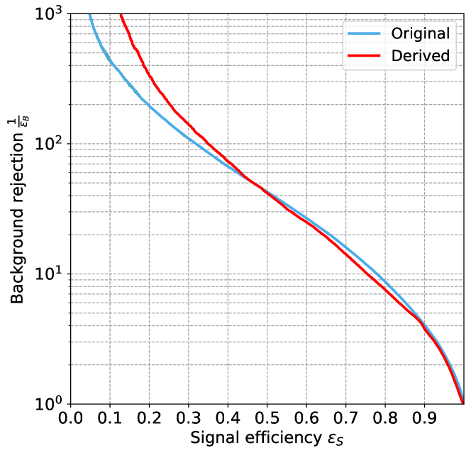
Figure 1: ROC curves of the LorentzNet classifier trained with the publicly available dataset (blue) and our generated dataset (red).

Dataset	Accuracy	AUC	$1/\epsilon_{B}(\epsilon_{s}=0.5)$	$1/\epsilon_{B}(\epsilon_{s}=0.7)$
Original	0.8439	0.916	42.57 $\pm$ 0.18	15.97 $\pm$ 0.12
Derived	0.834	0.9089	41.79	14.14

Table 1: Performance comparison between LorentzNet trained with the publicly available dataset and our generated dataset.

3 Model

As outlined in the introduction, we aim to demonstrate the effectiveness of capsules in enhancing the performance of GNNs. To serve our purpose, we choose to work with the LorentzNet architecture Gong:2022lye , augmenting it with an additional capsule block as the decoding block of the network. In the following, we will briefly review LorentzNet and the capsule block.

3.1 The LorentzNet block

LorentzNet is a permutation equivariant and Lorentz equivariant Graph Neural Network (GNN). It follows the universal approximation theorem villar2023scalars to construct Lorentz group equivariant continuous mappings. LorentzNet takes as input the jet constituents’ four vectors ($x_{i}$) and the associated scalars ($h_{i}$). In the original architecture, these scalars were constructed by one-hot encoding of particle identification (PID). For our analysis, we have also included ten additional HLFs (See section 2) as global variables. These inputs are made to pass through an input layer that projects these scalars into a higher dimensional latent space.

The building block of LorentzNet is called the Lorentz Group Equivariant Block (LGEB). It receives the output of the input layer and processes it further. The main action of the LGEBs can be summarised in three steps. Firstly, it utilizes the node embedding scalars, the Minkowski dot products, and the Minkowski norms of the jet constituent four vectors to construct the edge functions between nodes. Next, it uses these edge functions to construct the Minkowski dot product attention, aggregating the neighborhood four vectors and updating the node coordinates. Finally, it aggregates the neighborhood edge functions by weighting them by an edge-significance measure and updates the node embedding scalars. In LorentzNet, several LGEBs are used in series. If we denote the output of the $l$th LGEB as ($x^{l},h^{l}$), then the action of the $(l+1)$th LGEB can be summarised as Gong:2022lye :

$$m_{ij}^{l} =\phi_{e}\left(h_{i}^{l},h_{j}^{l},\psi(||x_{i}^{l}-x_{j}^{l}||^{2},\psi(\langle x_{i}^{l},x_{j}^{l}\rangle))\right)$$ (4)

$$x_{i}^{l+1} =x_{i}^{l}+c\sum_{j\in[N]}\phi_{x}(m_{ij}^{l}).x_{j}$$ (5)

$$h_{i}^{l+1} =h_{i}^{l}+\phi_{h}\left(h_{i}^{l},\sum_{j\in[N]}w_{ij}m_{ij}^{l}\right)$$ (6)

where, $w_{ij}=\phi_{m}(m_{ij}^{l})$ characterize the significance of the neighboring edges, ($\phi_{x},\phi_{e},\phi_{h},\phi_{m}$) are neural networks, $\psi(x)=sign(x)log(|x|+1)$ is a normalizing function and c is a constant introduced to prevent the scale of $x_{i}$ from exploding. In the original paper, the model was constructed with six LGEBs. We found five such blocks are enough for our study. We encourage the interested reader to consult ref Gong:2022lye for details on the architecture.

In the original LorentzNet model, the output of the LGEBs is passed through a decoding layer where the node embeddings ($h$’s) of the final LGEB undergo a global average pooling followed by two fully connected layers with dropout and a final softmax function to generate the classification prediction. For our analysis, we completely removed this decoding layer, replacing it with a fully connected layer. The output of this fully connected layer then passes through the capsule block to generate model predictions.

3.2 The Capsule block

Capsule Network (CapsNet) sabour2017dynamic was originally introduced as an upgraded version of CNNs for image analysis. They have proved quite effective in the analysis of overlapping images. However, as obvious from the previous discussion, we propose using capsules alongside GNNs for object-level prediction tasks. Below, we provide a brief overview of capsules and the design details of the capsule block used in our analysis.//

The key feature of capsules is that they are vector neurons where the length of the capsule gives the probability of the presence of a given object. At the same time, its orientation represents the different features of the object. A dynamic routing mechanism ensures that the output of the capsule in the lth layer is sent to the appropriate parent in the (l+1)th layer. Say, $u_{i}$ denotes the output of capsule $i$ in the lth layer. This output is multiplied with a learnable weight matrix to produce the prediction vectors $\hat{u}_{j|i}$ for the jth capsule in the (l+1)th layer. i.e., sabour2017dynamic

$$\hat{u}_{j|i}=W_{ij}u_{i}$$ (7)

A weighted sum is performed on the prediction vectors to determine the input $s_{j}$ of the next layer capsules sabour2017dynamic .

$$s_{j}=\sum_{i}c_{ij}\hat{u}_{j|i}$$ (8)

Here $c$s are the coupling coefficients that sum to one between a capsule $i$ in the lth layer and all capsules $j$ in the (l+1)th layer, i.e., $\sum_{j}c_{ij}=1$. This is ensured by expressing these coefficients as $Softmax(b_{ij})$, where $b_{ij}$s are determined following an iterative procedure. Initially, the logits $b_{ij}$ are initiated to zero so that each capsule in the lth layer is connected with all capsules in the next layer with equal weightage. with these initial logits, the initial coupling coefficient $c$’s and (l+1)th layer input $s$’s are computed. These $s_{j}$ undergo a squashing procedure to calculate the initial output $v_{j}$ of the jth capsule in the (l+1)th layer sabour2017dynamic .

$$v_{j}=\frac{||s_{j}||^{2}}{1+||s_{j}||^{2}}\frac{s_{j}}{||s_{j}||}$$ (9)

This ensures that capsules with small lengths shrink to zero and longer capsules attain a length closer to unity. These output $v_{j}$’s are used to update the initial logits $b_{ij}$s by encoding the agreement between the output of the lth layer $\hat{u}_{j|i}$ and the output of the (l+1)th layer $v_{j}$. i.e., sabour2017dynamic

$$b_{ij}=b_{ij}+\hat{u}_{j|i}.v_{j}$$ (10)

In other words, the coupling of parent capsule $j$ with the capsule $i$ in the lth layer increases when this dot product is large. This procedure is repeated a predetermined number of times, and the final output $v$s are used for further analysis.

As mentioned at the beginning of this section, the length of the capsule represents the probability that the input belongs to a given class. This is ensured by an appropriate choice of the loss function. For each class $k$, the margin loss has the form sabour2017dynamic :

$$L_{k}=T_{k}max(0,m^{+}-||v_{k}||)^{2}+\lambda(1-T_{k})max(0,||v_{k}||-m^{-})^{2}$$ (11)

where $\lambda$ is a weighting parameter. we follow the original work sabour2017dynamic and choose $m^{+}=0.9$, $m^{-}=0.1$, and $\lambda=0.5$. In addition to the margin loss, a reconstruction loss term introduces additional regularisation into the training process. In the original work, the output capsules were decoded to reproduce the original image, and the reconstruction loss quantifies the discrepancy between the original and reconstructed image. For our analysis, we use the jet-level high-level features as the analog of the image. The decoding layer of the capsule block tries to reconstruct these jet-level features and matches them with the input values. This step ensures that the network learns these important characteristics of the jet, enhancing its performance.

The implementation of the capsule block is similar to that suggested in reference sabour2017dynamic . The major difference is in the input to the capsule block. The original architecture used CNNs to generate this input; hence, the capsules’ inputs are images represented in the latent space. The capsule layers in reference sabour2017dynamic use convolution operations to process these images. In our case, the output of LorentzNet can be viewed as a linear array of numbers. To handle these, we have replaced the convolution layers of reference sabour2017dynamic with fully connected layers. The rest of the architecture is almost similar to reference sabour2017dynamic . We have one primary capsule layer accepting the output of LorentzNet. The output of LorentzNet has a shape $102\times 72$, where the number 102 corresponds to the jet constituents, and 72 represents the number of hidden dimensions. The action of the primary capsule layer results in $32\times 36$ 8-dimensional capsules. To achieve this, it first uses a fully connected layer that converts $102\times 72\rightarrow 102\times 36$. After this operation, it uses eight fully connected layers for the transformation $102\times 36\rightarrow 32\times 36$ and combines all these outputs. These are the $u_{i}$s mentioned earlier. The secondary capsule layer has two capsules (corresponding to the signal and background classes) of dimension eight. These capsules receive input from all capsules from the primary layer. They utilize the iterative routing mechanism discussed earlier to generate the output $v_{j}$s. Finally, we have the decoding layer that uses the output of the secondary capsules to reconstruct the jet-level features. We implement this decoding layer using three fully connected neural networks. We have made the model and our results available in the public repository: https://github.com/rama726/CapsLorentzNet.git. The interested reader is encouraged to consult the code for fine details regarding the architecture.

We implemented the CapsLorentzNet with PyTorch and trained it on a cluster with four Nvidia Tesla K80 GPUs. We pass the data in batches of size 32 on each GPU. The model is trained for a total of 35 epochs. At the end of each epoch, we test the model performance with the validation dataset, and the one with the best validation accuracy is saved for testing. For the optimizer and learning rate scheduler, we have followed the prescription of reference Gong:2022lye . We have used the ADAMW loshchilov2019decoupled optimizer with a weighted decay of 0.01. For the details on the learning rate scheduler, see ref Gong:2022lye .

4 Classifier Performance

This section will focus on discussing the performance of the CapsLorentzNet architecture. Before discussing our final results, we would like to check how much gain in performance can be achieved if we include these jet-level features (See Section 2) in the LorenzNet itself without making any architectural changes. In other words, we want to use these jet-level features as additional global variables in the node embedding along with the PID of each constituent. These jet-level inputs will be the same for all nodes of a graph and will represent the global characteristics of the graph.

We present our results in Figure 2 and Table 2. Here, we have denoted the classifier trained with additional global observables as LorentzNet-Global. As can be seen from the results, the inclusion of these additional features is unable to provide any improvement to the classifier’s performance. This is happening because the classifier is treating these jet-level features on the same footing as the PID information of the constituents without understanding their importance for the classification task at hand. We need some mechanism to instruct the classifier to pay special attention to these features. This is achieved through the inclusion of the regularisation by reconstruction mechanism in CapsLorentzNet.

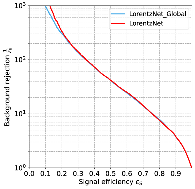
Figure 2: ROC curves of the LorentzNet classifier with (blue) and without (red) jet-level global observables.

Model	Accuracy	AUC	$1/\epsilon_{B}(\epsilon_{s}=0.5)$	$1/\epsilon_{B}(\epsilon_{s}=0.7)$
LorentzNet	0.834	0.9089	41.79	14.14
LorentzNet-Global	0.837	0.9087	41.55	13.91

Table 2: Performance comparison between LorentzNet trained with PID information of jet constituents as node embeddings and LorentzNet-Global that also includes additional jet-level observables in the node embeddings.

Now that the necessity of CapsLorentzNet architecture has been established, we will proceed to present the model’s performance on the quark-gluon dataset. In figure 3, we present the ROC curve of the CapsLorentzNet classifier. For comparison, we have also presented the performance of the original LorentzNet architecture on the same figure. Note that the results for CapsLorentzNet represent the average over six random initializations of the seeds. For consistent comparison, we have also presented some important matrices in table 3. A comparison of background rejection at 50% signal efficiency demonstrates that CapsLorentzNet can achieve almost 20 % performance gain compared to LorentzNet. This performance enhancement may not look that impressive. But notice that the current state-of-the-art architecture for quark-gluon tagging, ParT Qu:2022mxj , has a background rejection of 47.9 $\pm$ 0.5 at 50 % signal efficiency. If we take these numbers at face value, then CapsLorentzNet will be the current state of the art. But remember that although both parT and CapsLorentzNet are trained on similarly generated datasets, the datasets are not identical. A consistent comparison would require both models to be trained on the same dataset. The motivation behind this article is to demonstrate the usefulness of the architectural modification introduced in section 3 and not to present any state-of-the-art architecture. So, we refrain from presenting any such comparison. At the same time, we have made our code and dataset public , and any interested reader is welcome to do such a comparison.

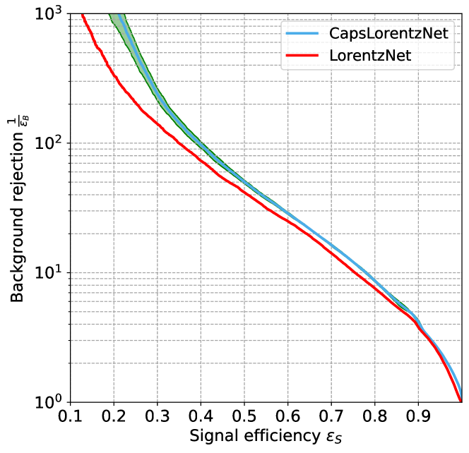
Figure 3: ROC curves of the LorentzNet (red) and CapsLorentzNet(blue) Classifiers. The results of CapsLorentzNet are averaged over six random initializations of the seeds.

Model	Accuracy	AUC	$1/\epsilon_{B}(\epsilon_{s}=0.5)$	$1/\epsilon_{B}(\epsilon_{s}=0.7)$
LorentzNet	0.834	0.9089	41.79	14.14
CapsLorentzNet	0.84303 $\pm$ 0.0009	0.91987 $\pm$ 0.0011	50.26 $\pm$ 1.43	16.36 $\pm$ 0.27

Table 3: Performance comparison between LorentzNet and CapsLorentzNet. The results of CapsLorentzNet are averaged over six random initializations of the seeds.

5 Summary and Outlook

This article proposes a new and innovative architectural modification that can be incorporated into most GNN architectures. It advocates replacing the final fully connected layers of any GNN architecture (decoding block) with capsules. This allows the scalar activations of the decoding blocks to be replaced with vector activation of the capsules. The orientation of these vectors represents important characteristics of the objects under study, and the magnitude characterizes whether the object belongs to the class the capsule represents. The regularisation by reconstruction mechanism of the capsule network provides a means to consistently incorporate High-Level Features into the analysis along with the usual low-level inputs of the GNNs. We have demonstrated the effectiveness of this strategy with the LorentzNet architecture for quark-gluon tagging. Our analysis shows a performance gain of around 20 % can be achieved with this strategy. This novel architectural modification can be extended to any other GNN architecture, and we believe similar performance gains can be achieved in all of these cases.

References

- (1) J. Cogan, M. Kagan, E. Strauss, and A. Schwarztman, Jet-Images: Computer Vision Inspired Techniques for Jet Tagging, JHEP 02 (2015) 118, [arXiv:1407.5675].
- (2) L. de Oliveira, M. Kagan, L. Mackey, B. Nachman, and A. Schwartzman, Jet-images — deep learning edition, JHEP 07 (2016) 069, [arXiv:1511.05190].
- (3) P. Baldi, K. Bauer, C. Eng, P. Sadowski, and D. Whiteson, Jet Substructure Classification in High-Energy Physics with Deep Neural Networks, Phys. Rev. D 93 (2016), no. 9 094034, [arXiv:1603.09349].
- (4) J. Barnard, E. N. Dawe, M. J. Dolan, and N. Rajcic, Parton Shower Uncertainties in Jet Substructure Analyses with Deep Neural Networks, Phys. Rev. D 95 (2017), no. 1 014018, [arXiv:1609.00607].
- (5) P. T. Komiske, E. M. Metodiev, and M. D. Schwartz, Deep learning in color: towards automated quark/gluon jet discrimination, JHEP 01 (2017) 110, [arXiv:1612.01551].
- (6) ATLAS Collaboration, Quark versus Gluon Jet Tagging Using Jet Images with the ATLAS Detector, .
- (7) G. Kasieczka, T. Plehn, M. Russell, and T. Schell, Deep-learning Top Taggers or The End of QCD?, JHEP 05 (2017) 006, [arXiv:1701.08784].
- (8) W. Bhimji, S. A. Farrell, T. Kurth, M. Paganini, Prabhat, and E. Racah, Deep Neural Networks for Physics Analysis on low-level whole-detector data at the LHC, J. Phys. Conf. Ser. 1085 (2018), no. 4 042034, [arXiv:1711.03573].
- (9) S. Macaluso and D. Shih, Pulling Out All the Tops with Computer Vision and Deep Learning, JHEP 10 (2018) 121, [arXiv:1803.00107].
- (10) J. Guo, J. Li, T. Li, F. Xu, and W. Zhang, Deep learning for -parity violating supersymmetry searches at the LHC, Phys. Rev. D 98 (2018), no. 7 076017, [arXiv:1805.10730].
- (11) F. A. Dreyer, G. P. Salam, and G. Soyez, The Lund Jet Plane, JHEP 12 (2018) 064, [arXiv:1807.04758].
- (12) D. Guest, J. Collado, P. Baldi, S.-C. Hsu, G. Urban, and D. Whiteson, Jet Flavor Classification in High-Energy Physics with Deep Neural Networks, Phys. Rev. D 94 (2016), no. 11 112002, [arXiv:1607.08633].
- (13) G. Louppe, K. Cho, C. Becot, and K. Cranmer, QCD-Aware Recursive Neural Networks for Jet Physics, JHEP 01 (2019) 057, [arXiv:1702.00748].
- (14) T. Cheng, Recursive Neural Networks in Quark/Gluon Tagging, Comput. Softw. Big Sci. 2 (2018), no. 1 3, [arXiv:1711.02633].
- (15) S. Egan, W. Fedorko, A. Lister, J. Pearkes, and C. Gay, Long Short-Term Memory (LSTM) networks with jet constituents for boosted top tagging at the LHC, arXiv:1711.09059.
- (16) K. Fraser and M. D. Schwartz, Jet Charge and Machine Learning, JHEP 10 (2018) 093, [arXiv:1803.08066].
- (17) L. G. Almeida, M. Backović, M. Cliche, S. J. Lee, and M. Perelstein, Playing Tag with ANN: Boosted Top Identification with Pattern Recognition, JHEP 07 (2015) 086, [arXiv:1501.05968].
- (18) J. Pearkes, W. Fedorko, A. Lister, and C. Gay, Jet Constituents for Deep Neural Network Based Top Quark Tagging, arXiv:1704.02124.
- (19) A. Butter, G. Kasieczka, T. Plehn, and M. Russell, Deep-learned Top Tagging with a Lorentz Layer, SciPost Phys. 5 (2018), no. 3 028, [arXiv:1707.08966].
- (20) T. Roxlo and M. Reece, Opening the black box of neural nets: case studies in stop/top discrimination, arXiv:1804.09278.
- (21) K. Datta and A. Larkoski, How Much Information is in a Jet?, JHEP 06 (2017) 073, [arXiv:1704.08249].
- (22) J. A. Aguilar-Saavedra, J. H. Collins, and R. K. Mishra, A generic anti-QCD jet tagger, JHEP 11 (2017) 163, [arXiv:1709.01087].
- (23) H. Luo, M.-x. Luo, K. Wang, T. Xu, and G. Zhu, Quark jet versus gluon jet: fully-connected neural networks with high-level features, Sci. China Phys. Mech. Astron. 62 (2019), no. 9 991011, [arXiv:1712.03634].
- (24) L. Moore, K. Nordström, S. Varma, and M. Fairbairn, Reports of My Demise Are Greatly Exaggerated: -subjettiness Taggers Take On Jet Images, SciPost Phys. 7 (2019), no. 3 036, [arXiv:1807.04769].
- (25) K. Datta and A. J. Larkoski, Novel Jet Observables from Machine Learning, JHEP 03 (2018) 086, [arXiv:1710.01305].
- (26) P. T. Komiske, E. M. Metodiev, and J. Thaler, Energy flow polynomials: A complete linear basis for jet substructure, JHEP 04 (2018) 013, [arXiv:1712.07124].
- (27) P. T. Komiske, E. M. Metodiev, B. Nachman, and M. D. Schwartz, Pileup Mitigation with Machine Learning (PUMML), JHEP 12 (2017) 051, [arXiv:1707.08600].
- (28) J. Brehmer, K. Cranmer, G. Louppe, and J. Pavez, Constraining Effective Field Theories with Machine Learning, Phys. Rev. Lett. 121 (2018), no. 11 111801, [arXiv:1805.00013].
- (29) J. Brehmer, K. Cranmer, G. Louppe, and J. Pavez, A Guide to Constraining Effective Field Theories with Machine Learning, Phys. Rev. D 98 (2018), no. 5 052004, [arXiv:1805.00020].
- (30) J. D’Hondt, A. Mariotti, K. Mimasu, S. Moortgat, and C. Zhang, Learning to pinpoint effective operators at the LHC: a study of the signature, JHEP 11 (2018) 131, [arXiv:1807.02130].
- (31) J. H. Collins, K. Howe, and B. Nachman, Anomaly Detection for Resonant New Physics with Machine Learning, Phys. Rev. Lett. 121 (2018), no. 24 241803, [arXiv:1805.02664].
- (32) R. T. D’Agnolo and A. Wulzer, Learning New Physics from a Machine, Phys. Rev. D 99 (2019), no. 1 015014, [arXiv:1806.02350].
- (33) A. De Simone and T. Jacques, Guiding New Physics Searches with Unsupervised Learning, Eur. Phys. J. C 79 (2019), no. 4 289, [arXiv:1807.06038].
- (34) J. Hajer, Y.-Y. Li, T. Liu, and H. Wang, Novelty Detection Meets Collider Physics, Phys. Rev. D 101 (2020), no. 7 076015, [arXiv:1807.10261].
- (35) M. Farina, Y. Nakai, and D. Shih, Searching for New Physics with Deep Autoencoders, Phys. Rev. D 101 (2020), no. 7 075021, [arXiv:1808.08992].
- (36) T. Heimel, G. Kasieczka, T. Plehn, and J. M. Thompson, QCD or What?, SciPost Phys. 6 (2019), no. 3 030, [arXiv:1808.08979].
- (37) L. de Oliveira, M. Paganini, and B. Nachman, Learning Particle Physics by Example: Location-Aware Generative Adversarial Networks for Physics Synthesis, Comput. Softw. Big Sci. 1 (2017), no. 1 4, [arXiv:1701.05927].
- (38) M. Paganini, L. de Oliveira, and B. Nachman, Accelerating Science with Generative Adversarial Networks: An Application to 3D Particle Showers in Multilayer Calorimeters, Phys. Rev. Lett. 120 (2018), no. 4 042003, [arXiv:1705.02355].
- (39) L. de Oliveira, M. Paganini, and B. Nachman, Controlling Physical Attributes in GAN-Accelerated Simulation of Electromagnetic Calorimeters, J. Phys. Conf. Ser. 1085 (2018), no. 4 042017, [arXiv:1711.08813].
- (40) M. Paganini, L. de Oliveira, and B. Nachman, CaloGAN : Simulating 3D high energy particle showers in multilayer electromagnetic calorimeters with generative adversarial networks, Phys. Rev. D 97 (2018), no. 1 014021, [arXiv:1712.10321].
- (41) A. Andreassen, I. Feige, C. Frye, and M. D. Schwartz, JUNIPR: a Framework for Unsupervised Machine Learning in Particle Physics, Eur. Phys. J. C 79 (2019), no. 2 102, [arXiv:1804.09720].
- (42) P. Baldi, P. Sadowski, and D. Whiteson, Searching for Exotic Particles in High-Energy Physics with Deep Learning, Nature Commun. 5 (2014) 4308, [arXiv:1402.4735].
- (43) P. Baldi, P. Sadowski, and D. Whiteson, Enhanced Higgs Boson to Search with Deep Learning, Phys. Rev. Lett. 114 (2015), no. 11 111801, [arXiv:1410.3469].
- (44) J. Searcy, L. Huang, M.-A. Pleier, and J. Zhu, Determination of the polarization fractions in using a deep machine learning technique, Phys. Rev. D 93 (2016), no. 9 094033, [arXiv:1510.01691].
- (45) R. Santos, M. Nguyen, J. Webster, S. Ryu, J. Adelman, S. Chekanov, and J. Zhou, Machine learning techniques in searches for in the decay channel, JINST 12 (2017), no. 04 P04014, [arXiv:1610.03088].
- (46) E. Barberio, B. Le, E. Richter-Was, Z. Was, D. Zanzi, and J. Zaremba, Deep learning approach to the Higgs boson CP measurement in decay and associated systematics, Phys. Rev. D 96 (2017), no. 7 073002, [arXiv:1706.07983].
- (47) J. Duarte et al., Fast inference of deep neural networks in FPGAs for particle physics, JINST 13 (2018), no. 07 P07027, [arXiv:1804.06913].
- (48) M. Abdughani, J. Ren, L. Wu, and J. M. Yang, Probing stop pair production at the LHC with graph neural networks, JHEP 08 (2019) 055, [arXiv:1807.09088].
- (49) J. Lin, M. Freytsis, I. Moult, and B. Nachman, Boosting with Machine Learning, JHEP 10 (2018) 101, [arXiv:1807.10768].
- (50) Y. S. Lai, Automated Discovery of Jet Substructure Analyses, arXiv:1810.00835.
- (51) A. J. Larkoski, I. Moult, and B. Nachman, Jet Substructure at the Large Hadron Collider: A Review of Recent Advances in Theory and Machine Learning, Phys. Rept. 841 (2020) 1–63, [arXiv:1709.04464].
- (52) D. Guest, K. Cranmer, and D. Whiteson, Deep Learning and its Application to LHC Physics, Ann. Rev. Nucl. Part. Sci. 68 (2018) 161–181, [arXiv:1806.11484].
- (53) K. Albertsson et al., Machine Learning in High Energy Physics Community White Paper, J. Phys. Conf. Ser. 1085 (2018), no. 2 022008, [arXiv:1807.02876].
- (54) A. Radovic, M. Williams, D. Rousseau, M. Kagan, D. Bonacorsi, A. Himmel, A. Aurisano, K. Terao, and T. Wongjirad, Machine learning at the energy and intensity frontiers of particle physics, Nature 560 (2018), no. 7716 41–48.
- (55) S. Choi, S. J. Lee, and M. Perelstein, Infrared Safety of a Neural-Net Top Tagging Algorithm, JHEP 02 (2019) 132, [arXiv:1806.01263].
- (56) F. A. Dreyer and H. Qu, Jet tagging in the Lund plane with graph networks, JHEP 03 (2021) 052, [arXiv:2012.08526].
- (57) S. Gong, Q. Meng, J. Zhang, H. Qu, C. Li, S. Qian, W. Du, Z.-M. Ma, and T.-Y. Liu, An efficient Lorentz equivariant graph neural network for jet tagging, JHEP 07 (2022) 030, [arXiv:2201.08187].
- (58) A. Bogatskiy, B. Anderson, J. T. Offermann, M. Roussi, D. W. Miller, and R. Kondor, Lorentz Group Equivariant Neural Network for Particle Physics, arXiv:2006.04780.
- (59) H. Qu and L. Gouskos, ParticleNet: Jet Tagging via Particle Clouds, Phys. Rev. D 101 (2020), no. 5 056019, [arXiv:1902.08570].
- (60) E. A. Moreno, O. Cerri, J. M. Duarte, H. B. Newman, T. Q. Nguyen, A. Periwal, M. Pierini, A. Serikova, M. Spiropulu, and J.-R. Vlimant, JEDI-net: a jet identification algorithm based on interaction networks, Eur. Phys. J. C 80 (2020), no. 1 58, [arXiv:1908.05318].
- (61) V. Mikuni and F. Canelli, Point cloud transformers applied to collider physics, Mach. Learn. Sci. Tech. 2 (2021), no. 3 035027, [arXiv:2102.05073].
- (62) P. Konar, V. S. Ngairangbam, and M. Spannowsky, Energy-weighted message passing: an infra-red and collinear safe graph neural network algorithm, JHEP 02 (2022) 060, [arXiv:2109.14636].
- (63) C. Shimmin, Particle Convolution for High Energy Physics, 7, 2021. arXiv:2107.02908.
- (64) CMS Collaboration, A. M. Sirunyan et al., Identification of heavy, energetic, hadronically decaying particles using machine-learning techniques, JINST 15 (2020), no. 06 P06005, [arXiv:2004.08262].
- (65) Y.-L. Du, K. Zhou, J. Steinheimer, L.-G. Pang, A. Motornenko, H.-S. Zong, X.-N. Wang, and H. Stöcker, Identifying the nature of the QCD transition in relativistic collision of heavy nuclei with deep learning, Eur. Phys. J. C 80 (2020), no. 6 516, [arXiv:1910.11530].
- (66) J. Li, T. Li, and F.-Z. Xu, Reconstructing boosted Higgs jets from event image segmentation, JHEP 04 (2021) 156, [arXiv:2008.13529].
- (67) J. Filipek, S.-C. Hsu, J. Kruper, K. Mohan, and B. Nachman, Identifying the Quantum Properties of Hadronic Resonances using Machine Learning, arXiv:2105.04582.
- (68) E. Bols, J. Kieseler, M. Verzetti, M. Stoye, and A. Stakia, Jet Flavour Classification Using DeepJet, JINST 15 (2020), no. 12 P12012, [arXiv:2008.10519].
- (69) M. Erdmann, E. Geiser, Y. Rath, and M. Rieger, Lorentz Boost Networks: Autonomous Physics-Inspired Feature Engineering, JINST 14 (2019), no. 06 P06006, [arXiv:1812.09722].
- (70) E. A. Moreno, T. Q. Nguyen, J.-R. Vlimant, O. Cerri, H. B. Newman, A. Periwal, M. Spiropulu, J. M. Duarte, and M. Pierini, Interaction networks for the identification of boosted decays, Phys. Rev. D 102 (2020), no. 1 012010, [arXiv:1909.12285].
- (71) V. Mikuni and F. Canelli, ABCNet: An attention-based method for particle tagging, Eur. Phys. J. Plus 135 (2020), no. 6 463, [arXiv:2001.05311].
- (72) E. Bernreuther, T. Finke, F. Kahlhoefer, M. Krämer, and A. Mück, Casting a graph net to catch dark showers, SciPost Phys. 10 (2021), no. 2 046, [arXiv:2006.08639].
- (73) J. Guo, J. Li, T. Li, and R. Zhang, Boosted Higgs boson jet reconstruction via a graph neural network, Phys. Rev. D 103 (2021), no. 11 116025, [arXiv:2010.05464].
- (74) M. J. Dolan and A. Ore, Equivariant Energy Flow Networks for Jet Tagging, Phys. Rev. D 103 (2021), no. 7 074022, [arXiv:2012.00964].
- (75) G. E. Hinton, A. Krizhevsky, and S. D. Wang, Transforming auto-encoders, in Artificial Neural Networks and Machine Learning – ICANN 2011 (T. Honkela, W. Duch, M. Girolami, and S. Kaski, eds.), (Berlin, Heidelberg), pp. 44–51, Springer Berlin Heidelberg, 2011.
- (76) S. Sabour, N. Frosst, and G. E. Hinton, Dynamic routing between capsules, 2017.
- (77) R. Katebi, Y. Zhou, R. Chornock, and R. Bunescu, Galaxy morphology prediction using capsule networks, Monthly Notices of the Royal Astronomical Society 486 (Apr., 2019) 1539–1547.
- (78) V. Lukic, M. Brüggen, B. Mingo, J. H. Croston, G. Kasieczka, and P. N. Best, Morphological classification of radio galaxies: capsule networks versus convolutional neural networks, Monthly Notices of the Royal Astronomical Society 487 (May, 2019) 1729–1744.
- (79) S. Diefenbacher, H. Frost, G. Kasieczka, T. Plehn, and J. M. Thompson, CapsNets Continuing the Convolutional Quest, SciPost Phys. 8 (2020) 023, [arXiv:1906.11265].
- (80) Z. Xinyi and L. Chen, Capsule graph neural network, in International Conference on Learning Representations, 2019.
- (81) P. Komiske, E. Metodiev, and J. Thaler, Pythia8 quark and gluon jets for energy flow, May, 2019.
- (82) P. T. Komiske, E. M. Metodiev, and J. Thaler, Energy Flow Networks: Deep Sets for Particle Jets, JHEP 01 (2019) 121, [arXiv:1810.05165].
- (83) C. Bierlich et al., A comprehensive guide to the physics and usage of PYTHIA 8.3, SciPost Phys. Codeb. 2022 (2022) 8, [arXiv:2203.11601].
- (84) M. Cacciari, G. P. Salam, and G. Soyez, FastJet User Manual, Eur. Phys. J. C 72 (2012) 1896, [arXiv:1111.6097].
- (85) S. Villar, D. W. Hogg, K. Storey-Fisher, W. Yao, and B. Blum-Smith, Scalars are universal: Equivariant machine learning, structured like classical physics, 2023.
- (86) I. Loshchilov and F. Hutter, Decoupled weight decay regularization, 2019.
- (87) H. Qu, C. Li, and S. Qian, Particle Transformer for Jet Tagging, arXiv:2202.03772.