Dynamic Tuning Towards Parameter and Inference Efficiency for ViT Adaptation

Abstract

Existing parameter-efficient fine-tuning (PEFT) methods have achieved significant success on vision transformers (ViTs) adaptation by improving parameter efficiency. However, the exploration of enhancing inference efficiency during adaptation remains underexplored. This limits the broader application of pre-trained ViT models, especially when the model is computationally extensive. In this paper, we propose Dynamic Tuning (DyT), a novel approach to improve both parameter and inference efficiency for ViT adaptation. Specifically, besides using the lightweight adapter modules, we propose a token dispatcher to distinguish informative tokens from less important ones, allowing the latter to dynamically skip the original block, thereby reducing the redundant computation during inference. Additionally, we explore multiple design variants to find the best practice of DyT. Finally, inspired by the mixture-of-experts (MoE) mechanism, we introduce an enhanced adapter to further boost the adaptation performance. We validate DyT across various tasks, including image/video recognition and semantic segmentation. For instance, DyT achieves comparable or even superior performance compared to existing PEFT methods while evoking only $71\%-85\%$ of their FLOPs on the VTAB-1K benchmark.

1 Introduction

With the remarkable success of Vision Transformers (ViTs) [19, 48, 25], fine-tuing pre-trained ViT on other data domains [75] or task applications [74, 34, 54, 66] is becoming a common practice. However, as model sizes increase [73, 15, 47], the associated adaptation costs become prohibitive due to the burden of fine-tuning and inference on the target task. Parameter-efficient fine-tuning (PEFT) methods (e.g. AdaptFormer [10], LoRA [32], and VPT [34]), are proposed to tackle the tuning problem by reducing tunable model parameters. They usually update a small amount of parameters while keeping the original model fixed, which reduces learnable parameters effectively while maintaining fine-tuning accuracy.

Despite the extensive research in parameter efficiency, the inference efficiency on target tasks is less explored. We numerically demonstrate the inference efficiency of three representative PEFT methods in Figure. 1(a), revealing that none of them reduces the computation during inference compared to full tuning. This limitation poses challenges for adapting pre-trained ViT to downstream tasks, particularly when the model is computationally extensive. To this end, we aim to unify both parameter and inference perspectives for efficient ViT adaptations.

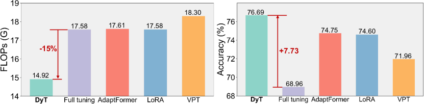
Figure 1: FLOPs and Accuracy of ViT-B/16 [19] on VTAB-1K [74]. “Full tuning” denotes that all parameters are trainable during fine-tuning. AdaptFormer [10], LoRA [32] and VPT [34] are typical PEFT methods.

Dynamic networks [69, 58, 44] demonstrate that token pruning helps to reduce model inference costs. However, these designs primarily focus on pre-training from scratch or full tuning on the same dataset, without considering data domain transfer. Furthermore, the token pruning operation constraints these methods on visual recognition scenarios, limiting their further applications e.g. dense prediction [77]. Our motivation thus arises from how to develop dynamic modules together with PEFT methods to enhance both parameter and inference efficiency during ViT adaptation, which should also suit a wide range of visual tasks.

In this paper, we introduce Dynamic Tuning (DyT), an efficient approach for ViTs adaptation that achieves both parameter and inference efficiency. Specifically, we design a token dispatcher for each transformer block learning to dynamically determine whether a token should be activated or deactivated. Only those activated tokens will traverse the entire block and an extra lightweight adapter module, while the remaining tokens skip the original block and will solely be processed by the adapter. DyT does not reduce the total number of tokens, making it suitable for both visual recognition and dense prediction scenarios. Additionally, since the impact of token skipping during adaptation has not been explored, we propose four model variants to determine the best practice for DyT. Finally, as the adapter module is set to process all the visual tokens, we propose a mixture-of-expert(MoE)-based adapter design that further enhances token processing with negligible additional FLOPs. Through these designs, our DyT fulfills both parameter and inference efficiency for ViTs adaptation.

Comprehensive evaluations for DyT are conducted from multiple perspectives. In the image domain, as shown in Figure 1(b). DyT surpasses existing PEFT methods while consuming only $85\%$ of the ViT-B FLOPs on the VTAB-1K benchmark [74]. When visual tokens are scaled up from images to videos, our DyT shows superior generalization ability on action recognition benchmarks, e.g. K400 [9] and SSV2 [24], with a reduction of 37GFLOPs. In the scenario where labels are scaled up from recognition to segmentation, our DyT even outperforms full tuning on ADE20K [77] with 21GFLOPs reduction. These experimental results indicate that the proposed DyT is efficient in both parameter and inference across various visual tasks and directs a promising field for efficient model adaptation.

2 Related Works

Parameter-efficient fine-tuning.

Parameter-efficient fine-tuning (PEFT) is designed to adapt a pre-trained model to downstream tasks by only tuning a small part of the parameters. Existing PEFT methods can broadly be categorized into three groups: adapter-based methods, re-parametrization-based methods, and prompt-based methods. Adapter-based methods [10, 31, 56, 36, 12] insert some tiny modules into the original model and only these inserted modules are updated during fine-tuning. Re-parametrization approaches [72, 32, 43, 20, 17] usually cooperate with reparameterization techniques, directly modifying specific parameters in the pre-trained model. Prompt-based methods [34, 2, 79, 78, 38, 8, 7] involve appending a small number of learnable tokens to input sequences, thereby adapting intermediate features in frozen layers. Please refer to [70, 42] to find more comprehensive reviews.

However, PEFT methods primarily focus on improving parameter efficiency during fine-tuning while overlooking inference cost reduction. In this paper, we propose to improve the parameter efficiency and address inference hosts simultaneously for efficient ViT adaptation.

Dynamic neural networks.

Dynamic neural networks[27] can dynamically adjust their architectures based on the input data, which enables them to control the computational redundancy based on input data. Existing methods have explored dynamic layer depth [61, 4, 68, 29, 26], dynamic channel width [30, 40, 28] and dynamic routing [41] in convolutional neural networks. When it comes to the era of vision transformer, many works [64, 60, 58, 44, 52] attempt to improve the inference efficiency by reducing the token redundancy. For instance, Liang et al. [44] identify and consolidate inattentive tokens into only one token in each transformer layer. Rao et al. [58] progressively discard less informative tokens between layers. Wang et al. [64] adjust the number of tokens to represent images. A more detailed literature review can be found in [27, 63]. Although these approaches have shown significant success in vision tasks, they require training a model from scratch or fine-tuning all parameters on the same dataset used in pre-training, making them unsuitable for efficient ViT adaptation.

In contrast to these methods, the proposed method can adapt pre-trained knowledge to diverse downstream datasets and tasks, while reducing the computational cost during inference by introducing negligible additional parameters.

3 ViTs Adaptation with Dynamic Tuning

In the following, we first introduce the vision transformer and the adapter architecture in Section 3.1. Subsequently, we present the proposed dynamic tuning (DyT) and explore its four variants in Section 3.2 and Section 3.3, respectively. Furthermore, we build an MoE-adapter, which effectively enhances the adaptation performance without introducing additional computational cost, as elaborated in Section 3.4. Finally, we introduce the loss functions of our method in Section 3.5.

3.1 Preliminary

Vision Transformer (ViT) consists of a stack of layers. The multi-head self-attention block denoted as $\operatorname{Attn}$, and multi-layer perceptron block, termed as $\operatorname{MLP}$ are the main components in each layer. The input of each layer can be denoted as $\mathbf{X}=[\mathbf{x}_{cls},\mathbf{x}_{1},\mathbf{x}_{2},...\mathbf{x}_{N}]\in\mathbb{R}^{(N+1)\times C}$, containing $N$ image tokens and a classification token $\mathbf{x}_{cls}$.

The adapter architectures have been widely explored in previous PEFT methods [10, 36, 31]. An adapter is generally designed as a bottleneck module, which consists of a project layer $\mathbf{W}_{down}\in\mathbb{R}^{C\times d}$ to squeeze the channel dimension and another project layer $\mathbf{W}_{up}\in\mathbb{R}^{d\times C}$ for dimension restoration. Here, $d$ denotes the bottleneck dimension and $d\ll C$ ensures the efficiency of the adapter. Given an input feature $\mathbf{X}$, the adapter operation is formulated as:

$$\mathbf{X}_{adapt}=\operatorname{Adapter}(\mathbf{X})=\sigma(\mathbf{X}\mathbf{W}_{down})\mathbf{W}_{up},$$ (1)

where $\sigma$ denotes a nonlinear function e.g. ReLU. In this study, we follow this general architecture to build the adapter within dynamic tuning. We place the adapter in parallel with an $\operatorname{Attn}$ block, $\operatorname{MLP}$, or an entire transformer layer, which will be presented in detail in Section 3.3.

3.2 Dynamic Tuning

In Vision Transformers (ViTs), the computational burden primarily resides in the transformer layers. Specifically, the operations in $\operatorname{Attn}$ and $\operatorname{MLP}$ account for approximately $35.8\%$ and $63.5\%$ of total FLOPs in ViT-B/16 [19]. Previous works [58, 44] have revealed that there exists a token-redundancy issue in ViTs and found that some tokens can be discarded without sacrificing the performance. Inspired by this, we propose an efficient ViT adaptation approach, named Dynamic Tuning (DyT), which not only maintains parameter efficiency during fine-tuning but also reduces redundant computation during inference. The core idea lies in dynamically selecting tokens for processing within transformer blocks. Given the input tokens $\mathbf{X}$ of a block, DyT can be formulated as:

$${\mathbf{X}^{\prime}}=\operatorname{Block}(\operatorname{TD}(\mathbf{X}))+\operatorname{Adapter}(\mathbf{X}),$$ (2)

where $\operatorname{Block}$ can represent an multi-head self-attention block $\operatorname{Attn}$, a multi-layer perceptron $\operatorname{MLP}$, or an entire transformer layer. The proposed token dispatcher ($\operatorname{TD}$) learns to selectively activate or deactivate tokens. Only the activated tokens are input into the $\operatorname{Block}$, while all tokens are processed by the $\operatorname{Adapter}$.

Token dispatcher.

The key point in DyT is to select partial tokens which will be passed through $\operatorname{Attn}$ and/or $\operatorname{MLP}$. A straightforward approach is randomly selecting tokens with a predefined probability and adapting the model to conduct downstream tasks with these selected tokens. However, this simplistic strategy risks discarding informative tokens while retaining less important tokens, potentially hindering the adaptation performance. To tackle this problem, we propose a token dispatcher (TD), which learns to select tokens during the adaptation. Specifically, given the input tokens $\mathbf{X}\in\mathbb{R}^{(N+1)\times C}$, $\operatorname{TD}$ learns to selectively activate a sequential of tokens $\mathbf{X}_{s}\in\mathbb{R}^{K\times C}$, where $K$ represents the number of activated tokens. To achieve this, it should obtain a mask $\mathbf{M}\in\mathbb{R}^{N+1}$, which indicates whether a token should be activated or deactivated.

To obtain $\mathbf{M}$, we adopt a projection layer $\mathbf{W}_{g}\in\mathbb{R}^{C\times 1}$ followed by a sigmoid function to predict the activation probability $\mathbf{S}\in\mathbb{R}^{N+1}$. Then, we set 0.5 as the threshold to determine the activation of each token. This can be formulated as:

$$\mathbf{S}=\operatorname{Sigmoid}(\mathbf{X}\mathbf{W}_{g}),\text{ }\mathbf{M}_{n}=\begin{cases}1&\text{ if }\mathbf{S}_{n}\geq 0.5\\ 0&\text{ if }\mathbf{S}_{n}<0.5\end{cases}\in\mathbf{M}.$$ (3)

$\mathbf{M}_{n}=1$ denotes that the $n$-th token is activated and will subsequently undergo the process of $\operatorname{Block}$. Conversely, if $\mathbf{M}_{n}=0$, the token will be deactivated and skip the $\operatorname{Block}$. In practice, we always set the mask value of the classification token $\mathbf{x}_{cls}$ to 1, allowing it to traverse the entire network. Notably, the number of additional parameters introduced in $\operatorname{TD}$ is negligible, with only $C$ parameters in the linear layer $\mathbf{W}_{g}$.

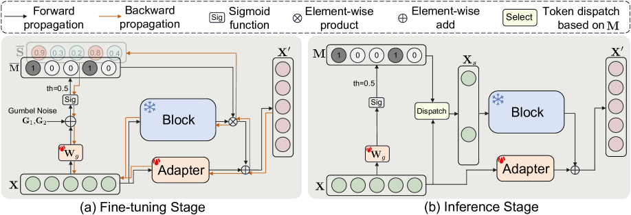
Figure 2: Overview of Dynamic Tuning. (a) In the fine-tuning stage, we adopt Gumbel Noise to enable end-to-end training. (b)In the inference stage, $\operatorname{TD}$ selects $K$ activated tokens $\mathbf{X}_{s}$ from $\mathbf{X}$ based on the mask $\mathbf{M}$, which saves the computations on those deactivated tokens in $\operatorname{Block}$. $\operatorname{Block}$ can represent a multi-head self-attention block $\operatorname{Attn}$, a multi-layer perceptron $\operatorname{MLP}$, or an entire transformer layer.

Fine-tuning stage.

However, directly using threshold makes $\mathbf{M}$ a discrete decision, resulting in a non-differentiable problem during fine-tuning. To address this, we incorporate the Gumbel Noise [30] into sigmoid to replace the original sigmoid function during fine-tuning. It can be formulated as:

$$\mathbf{\overline{S}}=\operatorname{Gumbel-Sigmoid}(\mathbf{X}\mathbf{W}_{g})=\operatorname{Sigmoid}(\frac{\mathbf{X}\mathbf{W}_{g}+\mathbf{G}_{1}-\mathbf{G}_{2}}{\tau}),$$ (4)

where $\mathbf{G}_{1}$, $\mathbf{G}_{2}\sim\operatorname{Gumbel}(0,1)$. $\tau$ represents the temperature and is set to 5.0 by default. Further details of Gumbel-Sigmoid are provided in the supplementary material. Subsequently, we can obtain $\mathbf{\overline{M}}$ using the same operation in Equation.3. The Gumbel Noise makes the sampling of $\mathbf{\overline{M}}$ stochastic during training and we adopt $\mathbf{\overline{S}}$ as a differentiable approximation of $\mathbf{\overline{M}}$. Both of these help $\operatorname{TD}$ to be trained in an end-to-end manner. The calculation of forward and backward propagations during training can be formulated as:

$$\mathbf{\overline{X}}_{s}=\begin{cases}\operatorname{Block}(\mathbf{X})\cdot\mathbf{\overline{M}}&\text{ Forward Propagation}\\ \operatorname{Block}(\mathbf{X})\cdot\mathbf{\overline{S}}&\text{ Backward Propagation}\end{cases},$$ (5)

The Equation 2 can be reformulated into:

$${\mathbf{X}^{\prime}}={\mathbf{X}}+\mathbf{\overline{X}}_{s}+\operatorname{Adapter}(\mathbf{X}),$$ (6)

From Equation 5, only the block outputs, $\operatorname{Block}(\mathbf{X})$, of those activated tokens are retained, while others are masked out by $\mathbf{\overline{M}}$. As shown in Figure 2 (a), during the fine-tuning stage, all tokens within $\mathbf{X}$ still need to traverse the $\operatorname{Block}$.

Inference stage.

During inference, we can directly adopt Equation 3 to generate the dispatch mask $\mathbf{M}$ and obtain activated tokens $\mathbf{X}_{s}\in\mathbb{R}^{K\times C}$ in $\operatorname{TD}$. Then, we can only feed them into $\operatorname{Block}$. Only processing $K$ tokens effectively reduces the computational cost because $K<N$. In practice, we add padding to the output from the $\operatorname{Block}$ to maintain tensor shape. This results in Equation 2. See Figure 2 (b) for a detailed illustration of the inference stage.

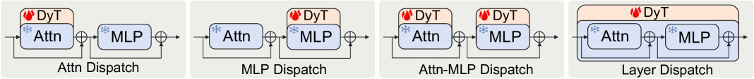
Figure 3: Model variants. For brevity, we omit the LayerNorm [1] in $\operatorname{Attn}$ and $\operatorname{MLP}$ blocks. “DyT” denotes the dynamic tuning presented in Figure 2.

3.3 Model Variants

The $\operatorname{Block}$ in Equation 2 can be instantiated into any blocks in the original ViT, such as a multi-head self-attention block $\operatorname{Attn}$, a multilayer perceptron block $\operatorname{MLP}$, or even a complete transformer layer in ViT. Since the impact of skipping tokens in these blocks during the adaptation fine-tuning remains non-trivial to estimate and has not been explored in previous works, we propose four model variants and conduct experiments to determine the best practice.

• Attention Dispatch: Considering the quadratic computational complexity of the $\operatorname{Attn}$ block with respect to the token numbers, skipping tokens before applying Attn can significantly reduce computation. In this design, multi-head self-attention is exclusively performed between activated tokens, while other tokens are bypassed, which may hurt the interaction between tokens.

• MLP Dispatch: Based on the analysis in Section 3.2, we observe that $\operatorname{MLP}$ takes $\sim$63.5% FLOPs in ViT-B/16 and propose to skip tokens only before $\operatorname{MLP}$. It enables that the interaction between tokens in $\operatorname{Attn}$ is not affected.

• Attention-MLP Dispatch: An alternative strategy is skipping tokens before both self-attention and MLP blocks. This design permits a higher activation rate in both $\operatorname{Attn}$ and $\operatorname{MLP}$ while maintaining similar computational efficiency comparable to “Attention Dispatch” and “MLP Dispatch”. However, it costs double the additional parameters in adapters.

• Layer Dispatch: Inspired by “Attention-MLP Dispatch”, we can dispatch tokens before a transformer layer. Specifically, tokens are identified by one $\operatorname{TD}$ to be activated or deactivated in the subsequent entire layer. With the same activation rate, its computation is similar to “Attention-MLP Dispatch” while requiring fewer parameters to build adapters.

We demonstrate the architecture variants in Figure 3. The experimental results and analyses of these variants are presented in Section 4.2.

3.4 MoE-Adapter

In DyT, the adapter is responsible for processing all tokens, requiring it to have enough capability, particularly when the downstream tasks e.g. semantic segmentation are challenging to adapt. To tackle this problem, we propose a MoE-adapter, inspired by mixture-of-experts [59, 67]. It effectively enhances the capability of the adapter with introducing negligible computation cost.

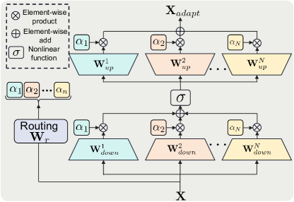
Figure 4: The architecture of the MoE-adapter. It is consist of $N$ adapter experts.

A MoE-adapter comprises a routing layer $\mathbf{W}_{r}\in\mathbb{R}^{C\times N}$ and $N$ adapter experts, denoted as $\{\mathbf{W}^{i}_{down}\in\mathbb{R}^{C\times d},\mathbf{W}^{i}_{up}\in\mathbb{R}^{d\times C}\}_{i=1}^{N}$. The routing layer generates a series of scalar as the weights for the experts based on input features. The features from different images may yield distinct expert weights. Specifically, we first conduct average pooling across all tokens to generate a feature as the global representation of them. Subsequently, this representation is fed into the routing layer to generate weight scalars $\{\alpha^{1},\alpha^{2},...\alpha^{N}\}$. Finally, tokens are processed by each expert independently and combined with the corresponding weight. We demonstrate this in Figure 4.

However, this increases the computational cost of the adapter in proportion to the number of experts $N$. To address this problem, we adopt its mathematical equivalence to process $\mathbf{X}$ in practice, which can be formulated as:

$$\mathbf{X}_{adapt}=\sigma(\mathbf{X}\mathbf{W}^{moe}_{down})\mathbf{W}^{moe}_{up},$$ (7)

where $\mathbf{W}^{moe}_{down}=\sum_{i=1}^{N}\alpha^{i}\mathbf{W}_{down}^{i}$ and $\mathbf{W}^{moe}_{up}=\sum_{i=1}^{N}\alpha^{i}\mathbf{W}_{up}^{i}$. The design endows the MoE-adapter with the same capacity as $N$ individual adapters, while maintaining computational efficiency equivalent to that of a single adapter (the computational cost in the routing layer is negligible).

3.5 Loss Functions

For an image $I$, we calculate the cross-entropy loss $\mathcal{L}_{cls}=-\mathbf{y}\operatorname{log}(\mathbf{\hat{y}})$ between the predicted probability $\mathbf{\hat{y}}$ and its corresponding one-hot label $\mathbf{y}$, to supervise the learning of classification. To control the average activation rate $r$ in the entire model, we add a loss term to constrain the number of activated tokens in the dynamic tuning, which can be formulated as:

$$\mathcal{L}_{rate}=(\frac{1}{L\times N}\sum_{l=1}^{L}\sum_{n=1}^{N}\mathbf{M}_{n}^{l}-r)^{2},$$ (8)

where $L$ denotes the number of layers in ViT. $\mathbf{M}_{n}^{l}$ represents the mask generated in $\operatorname{TD}$ from the $l$-th layer. Finally, the loss function is defined as $\mathcal{L}=\mathcal{L}_{cls}+\alpha\mathcal{L}_{rate}$, where $\alpha$ serves as the weight of the activation rate loss and is set to 2.0 by default.

4 Experiments

4.1 Experiment Settings

Datasets.

To evaluate the adaptation performance, we conduct experiments on VTAB-1K [74] benchmark. The training data in this benchmark is extremely limited, with only 1,000 training samples for each task. We also conduct experiments on three image classification datasets with complete training sets, including CIFAR-100 [39], SVHN [23], Food-101 [5]. We adopt two video datasets, Kinetic-400 (K400) [9] and Something-Something V2 (SSv2) [24], to evaluate the performance when the number of tokens scaled up. For the dense prediction task, we evaluate our method on two widely recognized semantic segmentation datasets, AED20K [77] and COCO-stuff [6].

Implementation Details.

We conduct all experiments based on the ViT-B/16 [19], which is pre-trained on ImageNet21K [16] with full supervision, unless otherwise specified. The bottleneck dimension $d$ is set to 64 by default. We adopt the same training schedule as [10]. Detailed hyperparameters for each experiment can be found in the supplementary material. The default setting in experiments is marked in color.

4.2 Analysis

Model variants.

In Table 1, we compare the performance of four model variants across both image and video datasets. We set the activation rate $r$ in “Attention Dispatch” and “MLP Dispatch” variants to 0.5, and to 0.7 for “Attention-MLP Dispatch” and “Layer Dispatch” variants, and train each respectively. This results in similar average FLOPs for four variants. We observe that the default setting “MLP Dispatch” achieves superior performance across four datasets while maintaining the lowest computational cost. Although “Attention-MLP Dispatch” and “Layer Dispatch” exhibit slightly better performance on K400, the former incurs double additional parameters while the latter lacks generalization capability on other datasets. The comparison between “MLP Dispatch” and other variants proves that only skipping tokens in MLP blocks is a better design.

In Figure 5, we further visualize the FLOPs-Accuracy curves of four model variants. We control the FLOPs by changing the activation rate $r$ for the fine-tuning stage. For “Attention Dispatch” and “MLP Dispatch”, we explore the activation rate in the range [0.1, 0.3, 0.5, 0.7, 0.9]. To maintain similar FLOPs as “Attention Dispatch” and “MLP Dispatch”, we adjust the activation rate for “Attention-MLP Dispatch” and “Layer Dispatch” within the range [0.5, 0.6, 0.7, 0.8, 0.9]. Across all datasets, “MLP Dispatch” consistently outperforms other variants. The performance of “Attn Dispatch” experiences a significant drop when the activation rate is lower than 0.9, which also indicates that skipping tokens for self-attention blocks in ViT is not a suitable way, due to the importance of the token mixing function of self-attention. Remarkably, “MLP Dispatch” can surpass full tuning with obviously fewer FLOPs on both CIFAR-100 and Food-101, further validating the effectiveness of our approach.

Table 1: Comparison of model variants. “Params. (M)” indicates the additional parameters in backbones. “FLOPs (G)” denotes the average FLOPs on CIFAR-100.

Model Variant	Params.(M) $\downarrow$	FLOPs (G) $\downarrow$	Image Accuracy (%) $\uparrow$			Video Accuracy (%) $\uparrow$
			CIFAR-100	SVHN	Food-101	K400	SSv2
Attention Dispatch	1.19	14.77	84.58	96.55	86.67	69.67	41.56
MLP Dispatch	1.19	12.21	91.37	97.08	90.32	74.39	45.34
Attention-MLP Dispatch	2.38	12.93	90.03	96.66	88.61	74.62	41.83
Layer Dispatch	1.19	13.08	89.38	96.57	89.05	74.72	43.94

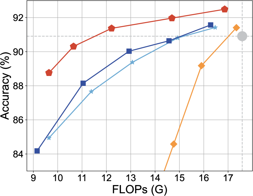
(a) CIFAR-100

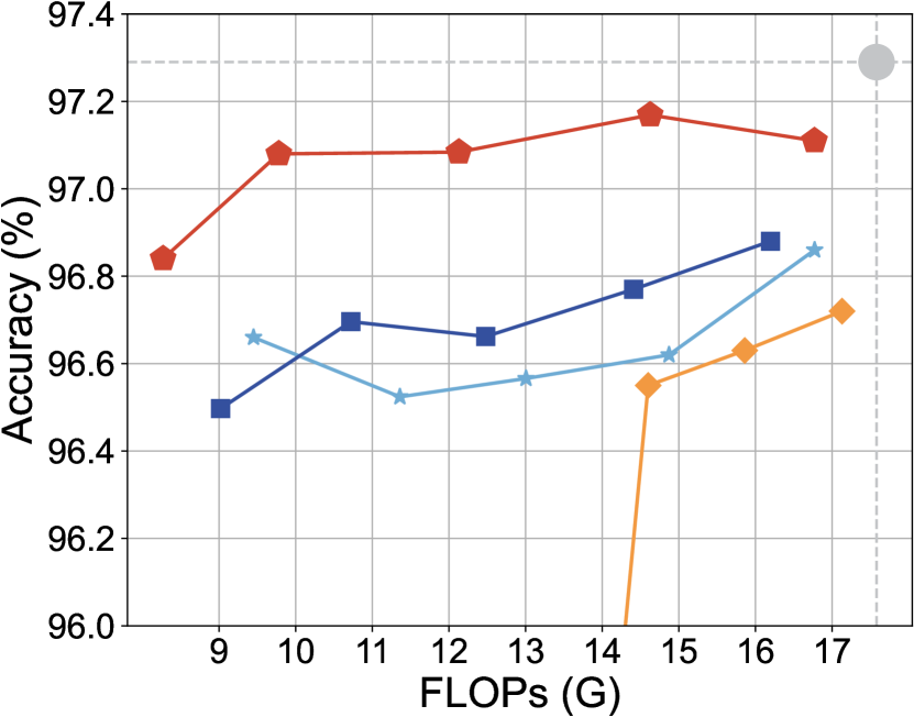
(b) SVHN

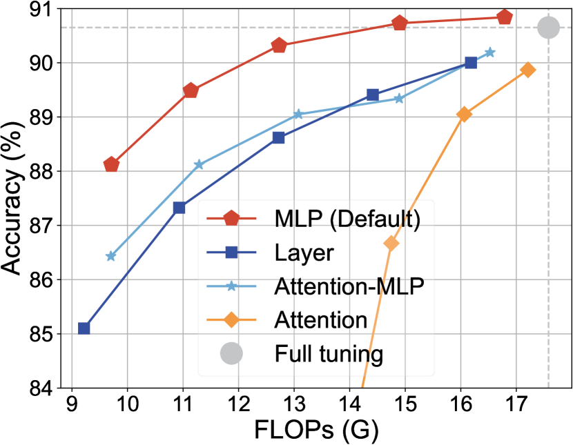
(c) Food-101

Figure 5: FLOPs-Accuracy curves of model variants on CIFAR100, SVHN, and Food-101 datasets. “MLP Dispatch” achieve the best FLOPs-Accuracy trade-off. We explore the activation rate $r$ within [0.1, 0.3, 0.5, 0.7, 0.9] for “Attention Dispatch” and “MLP Dispatch”. For “Attention-MLP Dispatch” and “Layer Dispatch” models, $r$ is adjusted within the range [0.5, 0.6, 0.7, 0.8, 0.9]. “Full tuning” denotes the traditional full fine-tuning approach. To conserve space, we use simplified names for the variants.

Investigations of dispatch level and dispatch strategy.

The proposed DyT performs dynamic dispatch at the token level using the token dispatcher (TD). In addition to token-level dispatch, we also investigate a sample-level dispatch, where all tokens within the selected samples are activated, while all tokens will be deactivated for other samples. To verify the importance of TD, we compare it against random dispatch, which randomly activates tokens or samples during both fine-tuning and inference. The experimental results are presented in Table 2.

Our observations reveal that token-level dispatch with TD consistently achieves superior performance across all datasets, except for a slight decrease compared to sample-level dispatch on the SVHN dataset. Notably, TD can achieve much better performance than the random dispatch strategy on both token-level and sample-level dispatch, particularly on video datasets K400 and SSv2, thereby validating the dispatch strategy learned in TD. Furthermore, the token-level dispatch surpasses the sample-level dispatch by a significant margin on most datasets, which demonstrates the importance of the finer-grained activation.

Table 2: Investigations of dispatch level and dispatch strategy. Combining the token-level dispatch and TD strategy results in the best performance. We consider two dispatch levels: “Token” (where dispatch is performed at the token-level) and “Sample” (where dispatch is conducted at the sample-level). “TD” and “Random” represent the learned dispatcher and random dispatch strategy, respectively.

Dispatch Level			Dispatch Strategy		Image Accuracy (%) $\uparrow$			Video Accuracy (%) $\uparrow$
Token	Sample	TD	Random	CIFAR-100	SVHN	Food-101	K400	SSv2
✓		✓		91.37	97.08	90.32	74.39	45.34
	✓	✓		90.70	97.29	89.8	71.14	44.09
✓			✓	89.38	96.79	86.39	68.27	40.13
	✓		✓	87.15	97.07	85.26	68.18	39.79

Different bottleneck dimensions.

We investigate the impact of the bottleneck dimensions of the adapter in DyT and the results are summarized in Table 3, revealing that different datasets prefer different configurations. When the dataset is easy to adapt, such as CIFAR-100, a bottleneck dimension of $d=4$ is sufficient to achieve satisfactory performance. Conversely, video datasets require larger adapter dimensions e.g. $d=256$ to attain better performance. We set the default bottleneck dimension to 64, which achieves a balance between performance and cost, such as the number of additional parameters and FLOPs. It is worth noting that the relationship between FLOPs and bottleneck dimension is not strictly monotonic. For instance, when $d=16$, the FLOPs are lower than when $d=1$, since the training may converge at activating fewer tokens as the number of adapter’s parameters increases.

Table 3: Different bottleneck dimensions. Different datasets prefer different bottleneck dimensions. $d=64$ strikes a balance between accuracy and cost, such as extra parameters and FLOPs. “FLOPs (G)” denotes the average FLOPs on CIFAR-100.

Dimension	Params. (M) $\downarrow$	FLOPs (G) $\downarrow$	Image Accuracy (%) $\uparrow$			Video Accuracy (%) $\uparrow$
			CIFAR-100	SVHN	Food-101	K400	SSv2
1	0.03	12.11	91.46	95.5	89.65	71.78	36.22
4	0.08	11.89	91.57	96.61	89.99	73.16	39.24
16	0.30	12.06	91.46	96.98	90.24	73.65	42.49
64	1.19	12.21	91.37	97.08	90.32	74.39	45.34
256	4.73	13.32	91.18	97.03	90.42	75.33	46.73

Effectiveness of MoE-adapter.

We conduct experiments to explore the effectiveness of the MoE-adapter and the results are illustrated in Table 4. The MoE-adapter design ensures that the FLOPs will theoretically remain the same as the ordinary adapter, with the computational cost from the routing function being negligible. However, in practical scenarios, the computational cost is also influenced by the learned token dispatch strategy within the Token Dispatcher (TD), leading to slightly varying FLOPs across different models in Table 4.

We observe that the performance on image datasets drops when we increase the expert number in MoE-adapter. This phenomenon can be attributed to the simplicity of image datasets and the model does not require too many parameters to adapt. In contrast, for video datasets, such as K400 and SSv2, the best accuracy is achieved with 4 and 8 experts, respectively. The reason behind this is that the domain gap between the pre-training dataset and video datasets is large and the model needs sufficient adapter capacity to learn the adaptation. This proves that we can introduce the MoE-adapter when the target dataset is difficult to adapt.

Table 4: Effectiveness of MoE-Adapter. DyT${\dagger}$ denotes the DyT with MoE-adapters. Ordinary adapter is enough to handle image datasets while MoE-adapter is more suitable for challenging scenarios, such as video datasets. It theoretically does not increase extra computational cost, but the FLOPs slightly vary in different models since the learned token dispatch strategy in the TD is different. $N$ represents the number of experts. “FLOPs (G)” denotes the average FLOPs measured on CIFAR-100.

Model	Params. (M) $\downarrow$	FLOPs (G) $\downarrow$	Image Accuracy (%) $\uparrow$			Video Accuracy (%) $\uparrow$
			CIFAR-100	SVHN	Food-101	K400	SSv2
DyT	1.19	12.21	91.37	97.08	90.32	74.39	45.34
DyT${\dagger}$ $N=2$	2.40	12.58	91.07	96.09	89.98	74.55	45.78
DyT${\dagger}$ $N=4$	4.80	12.29	91.01	96.90	89.77	75.00	46.56
DyT${\dagger}$ $N=8$	9.60	12.44	90.45	96.84	89.53	75.34	46.06
DyT${\dagger}$ $N=12$	14.40	12.43	90.31	96.72	89.32	75.17	44.97

Visualization of token activation rate in each layer.

In Figure 6, we visualize the token activation rates across different layers in ViT-B/16 [19]. We observe that the model tends to activate more tokens in lower layers while deactivating tokens in higher layers. This phenomenon can be attributed to that the model tends to take more general knowledge from the lower layers of the pre-trained model and learn more task-specific knowledge in higher levels. Additionally, the activation results vary across different datasets. For instance, SSv2 demonstrates increased token activation rate in Layer 5 and Layer 6 compared to other datasets, whereas SVHN experiences substantial token deactivation in Layer 6, 7, and 8. This discrepancy arises from that the model needs different knowledge from the pre-trained weights to address dataset-specific challenges.

It is noteworthy that nearly all tokens are deactivated in the final layer across five datasets, especially CIFAR-100, SVHN, and K400, where the activation rates are exactly 0%. This indicates that on these datasets, we can directly drop the original MLP block in Layer11 without hurting the performance, which further reduces about 4.7M , 26.6% of the ViT-B total parameters.

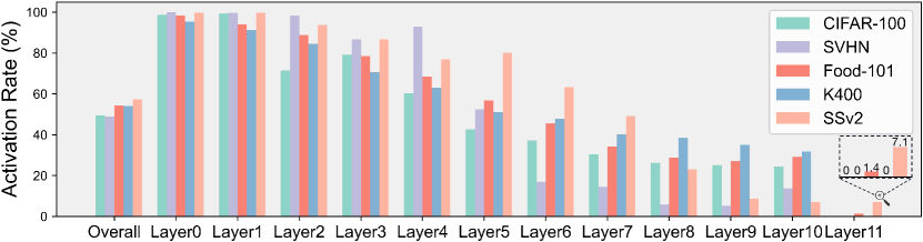
Figure 6: Token activation rate in different layers. We visualize the token activation rates from 12 layers in ViT-B/16. “Overall” denotes the mean activation rate in the whole model, which arrives at around 50% when $r$ is set to 0.5. “Layer0” and “Layer11” denote the lowest and highest level, respectively. Notably, the activation rate in the last layer is exactly 0% on CIFAR-100, SVHN, and K400 datasets..

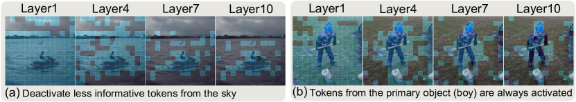
Figure 7: Visualization of activated tokens. We present two representative samples from the K400 dataset. Blue patches represent the tokens activated in token dispatcher (Detailed in Section 3.2). Results verify that the token dispatcher has learned to identify informative tokens during fine-tuning.

Visualization of activated tokens.

In Figure 7, we visualize two representative samples from K400. We can observe that the model tends to deactivate those tokens that are less informative e.g. tokens of the sky in (a) and tokens of grass in (b). In higher layers, such as layer7 and layer10, only those tokens from the primary objects are activated. This further proves the the existence of token redundancy problems in ViT and provides validation for the rationality behind our approach. Additional visualizations are available in the supplementary material.

4.3 VTAB-1K Results

To evaluate the adaptation performance when the training data is limited, we adapt the VTAB-1K [74] benchmark. Following exiting works, we reduce the bottleneck dimension $d$ to 8, resulting in only 0.16M extra parameters. We vary the activation rate $r$ in DyT in the range [0.5, 0.7, 0.9] and conduct fine-tuning, obtaining three models with different inference costs.

The results are presented in Table 5. Although previous methods, such as ConvPass [36] and Res-Tuning [35], achieve satisfactory performance, they do not improve the efficiency during inference and even introduce additional FLOPs compared with full fine-tuning. In contrast, with only 12.54 GFLOPs, about 71% of the cost in original ViT-B, our method has outperformed most previous methods e.g. LoRA [32] and VPT [34], by a large margin. Furthermore, as FLOPs increase, DyT continues to exhibit superior performance than other methods. These experimental results validate that DyT effectively improves parameter efficiency and inference efficiency while maintaining the adaptation performance.

Table 5: Performance and efficiency comparison on VTAB-1K. Our approach achieves significant adaptation performance while simultaneously enhancing both parameter and inference efficiency. “Group Mean” indicates the averaged accuracy of three groups. “Full tuning” indicates fine-tuning all parameters. “Frozen” means that all parameters in the backbone keep frozen. “Param. (M)” denotes the number of trainable parameters in backbones. “FLOPSs (G)” is the average FLOPs across all datasets. Bold font and underline denote the best and the second-best performance respectively.

	Natural							Specialized				Structured								Structured
	CIFAR-100	Caltech101	DTD	Flowers102	Pets	SVHN	Sun397	Camelyon	EuroSAT	Resisc45	Retinopathy	Clevr-Count	Clevr-Dist	DMLab	KITTI-Dist	dSpr-Loc	dSpr-Ori	sNORB-Azim	sNORB-Elev	Group Mean	Param. (M)	FLOPs (G)
Traditional methods
Full tuning	68.9	87.7	64.3	97.2	86.9	87.4	38.8	79.7	95.7	84.2	73.9	56.3	58.6	41.7	65.5	57.5	46.7	25.7	29.1	68.96	85.8	17.58
Frozen	63.4	85.0	63.2	97.0	86.3	36.6	51.0	78.5	87.5	68.6	74.0	34.3	30.6	33.2	55.4	12.5	20.0	9.6	19.2	57.64	0	17.58
Parameter-efficient tuning methods
Adapter [31]	69.2	90.1	68.0	98.8	89.9	82.8	54.3	84.0	94.9	81.9	75.5	80.9	65.3	48.6	78.3	74.8	48.5	29.9	41.6	73.85	0.16	17.61
BitFit [72]	72.8	87.0	59.2	97.5	85.3	59.9	51.4	78.7	91.6	72.9	69.8	61.5	55.6	32.4	55.9	66.6	40.0	15.7	25.1	65.21	0.10	17.58
LoRA [32]	67.1	91.4	69.4	98.8	90.4	85.3	54.0	84.9	95.3	84.4	73.6	82.9	69.2	49.8	78.5	75.7	47.1	31.0	44.0	74.60	0.29	17.58
VPT [34]	78.8	90.8	65.8	98.0	88.3	78.1	49.6	81.8	96.1	83.4	68.4	68.5	60.0	46.5	72.8	73.6	47.9	32.9	37.8	71.96	0.53	18.30
SSF [36]	69.0	92.6	75.1	99.4	91.8	90.2	52.9	87.4	95.9	87.4	75.5	75.9	62.3	53.3	80.6	77.3	54.9	29.5	37.9	75.69	0.20	17.58
NOAH [76]	69.6	92.7	70.2	99.1	90.4	86.1	53.7	84.4	95.4	83.9	75.8	82.8	68.9	49.9	81.7	81.8	48.3	32.8	44.2	75.48	0.36	17.58*
ConvPass [36]	72.3	91.2	72.2	99.2	90.9	91.3	54.9	84.2	96.1	85.3	75.6	82.3	67.9	51.3	80.0	85.9	53.1	36.4	44.4	76.56	0.33	17.64
AdaptFormer [10]	70.8	91.2	70.5	99.1	90.9	86.6	54.8	83.0	95.8	84.4	76.3	81.9	64.3	49.3	80.3	76.3	45.7	31.7	41.1	74.75	0.16	17.61
FacT-TT [37]	71.3	89.6	70.7	98.9	91.0	87.8	54.6	85.2	95.5	83.4	75.7	82.0	69.0	49.8	80.0	79.2	48.4	34.2	41.4	75.30	0.04	17.58
Res-Tuning [35]	75.2	92.7	71.9	99.3	91.9	86.7	58.5	86.7	95.6	85.0	74.6	80.2	63.6	50.6	80.2	85.4	55.7	31.9	42.0	76.32	0.51	17.67
The proposed Dynamic Tuning
DyT $r=0.5$	70.4	94.2	71.1	99.1	91.7	88.0	51.5	87.1	95.3	84.2	75.8	79.2	61.8	51.0	82.4	79.7	52.3	35.3	44.5	75.73	0.16	12.54
DyT $r=0.7$	73.9	94.9	72.1	99.4	91.8	88.4	55.5	87.2	95.6	86.2	75.9	80.3	61.8	51.7	83.1	81.6	53.7	35.3	45.2	76.69	0.16	14.92
DyT $r=0.9$	74.0	95.1	72.9	99.3	91.7	87.6	56.9	87.7	95.7	85.4	76.1	81.6	63.2	50.1	83.0	83.3	52.0	34.5	44.5	76.74	0.16	17.07

• NOAH cost larger than 17.58 FLOPS since it combines PEFT methods via neural architecture search.

4.4 Effectiveness on Image Datasets with Sufficient Training Data

Although the results from VTAB-1K have proven the superiority of our approach, we extend our investigation to complete image datasets, to evaluate the adaptation performance with sufficient training data. The results are demonstrated in Table 6. We further explore a straightforward approach, “Dynamic full tuning”, which has a token dispatcher as the same in DyT and is fine-tuned with all parameters. We observe that its performance becomes unstable and drops significantly on some datasets e.g. CIFAR-100 and Food101. This phenomenon may arise due to the potential adverse impact of dynamic dispatch on the pre-trained parameters during full-tuning adaptation, thereby validating the importance of DyT. In this data-sufficient scenario, although our method achieves performance slightly below that of full tuning and AdaptFormer, it brings a significant reduction in FLOPs.

4.5 Scaling Token Counts from Images to Videos

We conduct experiments on video datasets to show the performance when the number of tokens scaled up. The number of input frames is set to 8. For video tasks, similar to [71, 11], we employ a cross-attention layer and a query token to aggregate features from different frames. The video classification is conducted on the query token. Additional implementation details are provided in the supplementary material. We demonstrate the results in Table 6. Although DyT achieves slightly lower performance than AdaptFormer and LoRA, it costs obviously fewer FLOPs. DyT${\dagger}$ with four experts can achieve the best average accuracy, which further verifies the importance of capability in adapters.

4.6 Generalization on Semantic Segmentation

We also conduct experiments on two well-recognized semantic segmentation datasets ADE20K [77] and COCO-stuff [6] to demonstrate the ability of DyT on dense prediction tasks. Results are presented in Table 6. Following previous works [3, 18], we adopt the UperNet [65] as the segmentation head, and all images are resized into $512\times 512$. Training details can be found in the supplementary material. We observe that the computational cost of semantic segmentation is much higher than the image and video discrimination task, primarily due to the high-resolution feature maps. Both DyT and DyT${\dagger}$ still can reduce the computational cost obviously and achieve better performance than other PEFT methods, only slightly lower than full tuning on COCO-Stuff dataset.

Table 6: Results on three tasks. We present top-1 accuracy for both image and video datasets, while reporting mIOU scores for semantic segmentation datasets ADE20K and COCO-stuff. “Avg.” denotes the average results from the corresponding two datasets. The FLOPs are evaluated on CIFAR-100, K400 and ADE20K.

Method	Params. $\downarrow$	Image Datasets					Video Datasets				Semantic Segmentation Datasets
		FLOPs $\downarrow$	Image Accuracy (%)				FLOPs $\downarrow$	Video Accuracy (%)			FLOPs $\downarrow$	mIOU
	(M)	(G)	CIFAR-100	SVHN	Food101	Avg.	(G)	K400	SSv2	Avg.	(G)	ADE20K	COCO-stuff	Avg.
Traditional methods
Full tuning	85.80	17.58	90.91	97.29	90.69	92.96	142.53	75.48	45.22	60.35	605.36	47.66	45.89	46.78
Linear	0	17.58	85.87	56.29	88.07	76.74	142.53	69.04	27.64	48.34	605.36	43.86	44.46	44.16
Dynamic-Full	85.80	12.24	83.43	96.90	84.46	88.26	107.67	74.63	44.94	59.79	582.46	45.74	45.20	45.47
Parameter-efficient tuning methods
AdaptFormer [10]	1.19	17.81	92.03	97.23	90.84	93.36	144.39	75.53	45.36	60.45	606.57	47.52	45.33	46.43
LoRA [32]	1.19	17.58	91.42	97.36	90.48	93.08	142.53	75.48	45.62	60.55	605.36	47.34	45.53	46.44
VPT [34]	0.07	18.32	91.64	95.72	90.41	92.59	148.44	73.46	38.17	55.82	606.36	46.38	44.87	45.63
The proposed Dynamic Tuning
DyT	1.19	12.21	91.37	97.08	90.32	92.92	108.31	74.39	45.34	59.87	584.57	46.90	45.63	46.27
DyT${\dagger}$ $N=4$	4.80	12.29	91.01	96.90	89.77	92.56	105.45	75.00	46.56	60.78	584.40	47.67	45.71	46.69

5 Discussion and Conclusion

Previous methods for ViT adaptation primarily focus on improving the efficiency during the adaptation, thus aiming to reduce additional parameters. However, with the increasing size and computational cost of ViT models, the inference cost after the adaptation is becoming a heavy burden. In this paper, we unify both of these two problems into the efficiency problem for ViT adaptation and propose dynamic tuning (DyT) to tackle them simultaneously. We validate its performance and generalization across various tasks and datasets.

Limitations and future works. DyT is currently designed for vision tasks. We believe it would be interesting to combine vision backbones with large language models e.g. [62] to build efficient large multi-modal models e.g. [45, 80]. DyT could be further developed to be compatible with multi-modal models, which would be our future direction.

Appendix 0.A Appendix

0.A.1 Details about Gumbel-Sigmoid

Gumbel-Softmax is proposed in [33] to conduct the differentiable sampling from a distribution. Given an unnormalized log probability $\{\mathbf{E}_{i}\}_{i=1}^{N}$, the Gumbel-Softmax can be formulated as:

$$p_{i}=\frac{\exp\left(\left(\mathbf{E}_{i}+\mathbf{G}_{i}\right)/\tau\right)}{\sum_{n=1}^{N}\exp\left(\left(\mathbf{E}_{n}+\mathbf{G}_{n}\right)/\tau\right)},$$ (9)

where $\mathbf{G}_{i}$ denotes the Gumbel Noise sampled from a Gumbel distribution ($\mathbf{G}_{i}\sim\operatorname{Gumbel}(0,1)$). We can consider the special case, where $N=2$ and $E_{2}=0$, then $p_{1}$ can be defined as:

$$p_{1} =\frac{\exp\left(\frac{\mathbf{E}_{1}+\mathbf{G}_{1}}{\tau}\right)}{\exp\left(\frac{\mathbf{E}_{1}+\mathbf{G}_{1}}{\tau}\right)+\exp\left(\frac{\mathbf{G}_{2}}{\tau}\right)}$$ (10)

$$=\frac{1}{1+\exp\left(-\frac{\mathbf{E}_{1}+\mathbf{G}_{1}-\mathbf{G}_{2}}{\tau}\right)}$$ (11)

$$=\operatorname{Sigmoid}(\frac{\mathbf{E}_{1}+\mathbf{G}_{1}-\mathbf{G}_{2}}{\tau})$$ (12)

$$=\operatorname{Gumbel-Sigmoid}(\mathbf{E}_{1}),$$ (13)

obtaining the formulation of Gumbel-Sigmoid. Researchers in previous works, such as [22, 46], have also leveraged the Gumbel-Sigmoid formulation to facilitate end-to-end training of neural networks.

0.A.2 Implementation Details for each Task

Experimental settings on VTAB-1K.

Following previous works [36, 37, 35], we fine-tune the model for 100 epochs on each dataset in VTAB-1K [74]. We do not use any data augmentation strategy in these experiments. We adopt the AdamW [50] optimizer. The learning rate is set to 1e-3 and gradually decays to 0 based on a cosine schedule [49].

Experimental settings on complete image datasets.

We adopt the settings in Table 7 to fine-tune the ViT with the proposed dynamic tuning. Experiments on other parameter-efficiency methods such as AdaptFormer [10], LoRA [32], and VPT [34] also follow the settings in Table 7. When we train a model with full tuning, we adopt a 1/10 base learning rate to make the training stable, otherwise, the model can not achieve reasonable results.

Table 7: Experimental settings for complete image datasets. We present the hyperparameters in DyT. Following previous methods, we train the model with a 1/10 base learning rate in the full tuning setting. $lr=base\_lr\times batch\_size/256$

Configuration	CIFAR-100 [39], SVHN [23], Food-101 [5]
Optimizer	AdamW [50]
Base learning rate	1e-3
Weight decay	0.01
Batch size	1024
Training crop size	224
Learning rate schedule	Cosine decay [49]
GPU numbers	8
Warmup epochs	20
Training epochs	100
Augmentation	RandomResizedCrop

Experimental settings on video datasets.

We adopt two video datasets, Kinetic-400 (K400) [9] and Something-Something V2 (SSv2) [24], to evaluate the performance as the token count scales up. The experimental settings are demonstrated in Table 8. Most of the settings are borrowed from [54]. The number of input frames is set to 8. We adopt multi-view during the test, which is a common practice in video action recognition. However, the original ViT lacks temporal modeling capabilities. To address this limitation, we draw inspiration from [71, 11]. By introducing a cross-attention layer after the ViT, along with a query token, we effectively aggregate temporal information across different frames. The final video action classification is performed based on this query token. Experiments on parameter-efficient fine-tuning methods also follow these settings. We adopt a 1/10 base learning rate for those experiments on full tuning.

Table 8: Experimental settings for video datasets. We follow most of settings in [54]. The number of input frames is set to 8 in all experiments. $lr=base\_lr\times batch\_size/256$

Configuration	K400 [9]	SSV2 [24]
Optimizer	AdamW [50]
Base learning rate	1e-3
Weight decay	0.01
Batch size	128
Training Epochs	12	50
Training Resize	ShortSideJitter 224 - 256	RandomResizedCrop
Training crop size	224
Learning rate schedule	Cosine decay [49]
Frame sampling rate	16	dynamic, evenly covering the whole video
Mirror	✓	✗
RandAugment [14]	✗	✓
Num. testing views	1 spatial $\times$ 3 temporal	3 spatial $\times$ 1 temporal

Experimental settings on semantic segmentation datasets.

We conduct experiments on ADE20K [77] and COCO-stuff [6] to demonstrate the ability of DyT on dense prediction tasks. ADE20K contains 20,210 images from 150 fine-trained semantic concepts. COCO-Stuff consists of about 164k images with 172 semantic classes. The experimental settings are demonstrated in Table 9. All experiments for parameter-efficient fine-tuning methods also follow these settings. For the experiment on full tuning, we set adopt 1/10 learning rate for stable training and better performance.

Table 9: Experimental settings for semantic segmentation datasets. Following previous methods, we train the model with a 1/10 learning rate in the full tuning setting.

Configuration	ADE20K [77]	COCO-stuff [6]
Optimizer	AdamW [50]
Learning rate	1e-3
Weight decay	0.05
Batch size	16
Training crop size	512
Learning rate schedule	cosine decay [49]
Training iterations	160K	80K

0.A.3 More Experiments on Image Datasets

To reflect the performance when the training data is sufficient, we further conduct experiments on 6 datasets including CIFAR-10 [39], DTD [13], Aircraft [51], Flowers [53], Pet [55], and Car [21]. We report the top1 accuracy for CIFAR-10, Car, and DTD, while providing the mean class accuracy for the remaining datasets. The experimental settings also follow the Table 7

We find that DyT achieves comparable performance to full tuning and AdaptFormer [10], while reducing the computational cost significantly. Notably, the performance of dynamic full tuning is unstable on some datasets, such as Aircraft and Car. This phenomenon may be attributed to the dynamic token mechanism, which can potentially impact pre-trained parameters when all parameters are trainable. This further verifies the importance of the proposed dynamic tuning.

Table 10: Results on image datasets. “Dynamic full tuning” denotes that we fine-tuning all parameters in the original ViT with the proposed token dispatcher. “Frozen” means that all parameters in the backbone keep frozen. “Param. (M)” denotes the number of trainable parameters in backbones. “FLOPSs (G)” is the average FLOPs on CIFAR-10. Bold font and underline denote the best and the second-best performance respectively.

Method	Params. (M) $\downarrow$	FLOPs (G) $\downarrow$	Image Accuracy (%) $\uparrow$
			CIFAR-10	DTD	Aircraft	Flowers	Pet	Car
Traditional methods
Full tuning	85.80	17.58	98.76	74.52	80.53	99.00	93.11	88.71
Linear	0	17.58	96.70	73.67	40.51	99.03	92.78	52.85
Dynamic full tuning	85.80	12.15	97.16	54.15	62.50	61.34	75.16	70.48
Parameter-efficient tuning methods
AdaptFormer [10]	1.19	17.81	99.13	77.61	78.23	99.49	94.46	87.33
LoRA [32]	1.19	17.58	98.88	75.53	76.32	99.50	93.62	87.00
VPT [34]	0.07	18.32	98.75	72.66	68.91	99.35	93.92	80.72
The proposed DyT
DyT	1.19	11.41	98.72	75.00	78.33	99.36	93.92	87.90

0.A.4 Generalization Capability of Transformer Architecture

To verify the generalization of the proposed dynamic tuning, we conduct experiments based on Swin-B [48]. The dynamic tuning can be directly applied to MLP blocks in the swin transformer without any modifications. The bottleneck dimension $d$ of the adapter in dynamic tuning also is set to 64. The results are demonstrated in Table 11. We can observe that the dynamic tuning can reduce both the tunable parameters and FLOPs while achieving comparable or even better performance across three datasets. This verifies the generalization capability of the dynamic tuning.

Table 11: Generalization Capability on Swin Transformer [48]. The experiments are conducted based on Swin-B. “Param. (M)” denotes the number of trainable parameters in backbones. “FLOPs (G)” denotes the average FLOPs on CIFAR-100. The bottleneck dimension $d$ is set to 64.

Method	Params. (M) $\downarrow$	FLOPs (G) $\downarrow$	Image Accuracy (%) $\uparrow$
			CIFAR-100	SVHN	Food-101
Full tuning	86.74	15.40	91.82	97.66	93.05
DyT $r=0.1$	1.55	10.72	90.55	97.43	89.84
DyT $r=0.3$	1.55	12.07	91.26	97.38	90.66
DyT $r=0.5$	1.55	13.25	91.62	97.40	91.30
DyT $r=0.7$	1.55	14.05	92.14	97.21	91.96
DyT $r=0.9$	1.55	15.23	92.31	97.37	92.21

0.A.5 Scaling-up Model Size

We verify the effectiveness of dynamic tuning when the model size is scaled up. We conduct experiments on ViT-L [19] and compare dynamic tuning with full tuning. The bottleneck dimension $d$ of the adapter in dynamic tuning is also set to 64. The results are demonstrated in Table 12. We can observe that with the activation rate set to 0.3, DyT has outperformed “full tuning” obviously on both CIFAR-100 and Food-101, while resulting in significantly lower computational cost.

We further compare the proposed dynamic tuning with full tuning on the VTAB-1K benchmark [74]. The results are demonstrated in Table 13. With only 0.44M tunable parameters and 43.52 GFLOPs, dynamic tuning surpasses full tuning across most datasets and achieves much better average performance.

Table 12: Scale up the model size to ViT-L [19]. “Param. (M)” denotes the number of trainable parameters in backbones. “FLOPs (G)” denotes the average FLOPs on CIFAR-100. The default setting is marked in color. The bottleneck dimension $d$ is set to 64.

Method	Params. (M) $\downarrow$	FLOPs (G) $\downarrow$	Image Accuracy (%) $\uparrow$
			CIFAR-100	SVHN	Food-101
Full tuning	303.3	61.60	92.05	97.44	90.62
DyT $r=0.1$	3.17	32.56	91.26	97.04	89.98
DyT $r=0.3$	3.17	36.77	92.66	97.27	90.85
DyT $r=0.5$	3.17	43.79	93.49	97.38	91.49
DyT $r=0.7$	3.17	51.11	93.28	97.25	91.60
DyT $r=0.9$	3.17	60.05	93.44	97.23	91.59

Table 13: Performance and efficiency comparison on VTAB-1K. “Group Mean” indicates the averaged accuracy of three groups. “Full tuning” indicates fine-tuning all parameters. “Param. (M)” denotes the number of trainable parameters in backbones. “FLOPSs (G)” is the average FLOPs across all datasets. The bottleneck dimension is set to $d=8$.

	Natural							Specialized				Structured								Structured
	CIFAR-100	Caltech101	DTD	Flowers102	Pets	SVHN	Sun397	Camelyon	EuroSAT	Resisc45	Retinopathy	Clevr-Count	Clevr-Dist	DMLab	KITTI-Dist	dSpr-Loc	dSpr-Ori	sNORB-Azim	sNORB-Elev	Group Mean	Param. (M)	FLOPs (G)
Full tuning	69.5	96.2	73.8	98.8	90.7	91.6	44.8	85.8	96.2	87.8	75.3	83.0	62.0	50.8	80.0	85.8	54.6	29.7	35.4	75.7	303.3	61.60
DyT $r=0.5$	76.6	94.4	72.2	99.4	92.5	89.2	57.8	86.7	95.8	86.5	76.3	78.4	62.5	50.2	81.3	86.7	54.8	37.3	41.8	77.0	0.44	43.52

0.A.6 Investigation on the Temperature

We explore the temporal $\tau$ of the proposed dynamic tuning. The results are demonstrated in Table 14. When the temperature is smaller e.g. 0.1, the Gumbel Sigmoid tends to produce binary outputs close to 0 or 1. Conversely, larger temperatures lead to more uniform outputs, approaching 0.5. Results demonstrate that the performance is not too sensitive to the temperature and our model can achieve reasonable performance with all temperatures in the table. We also observe that the model with $\tau=1$ achieves the best performance on CIFAR-100, SVHN, and SSv2, while decaying the temperature with a schedule leads to the best result on Food-101 and K400, which shows that adjusting the temperature can help the model to achieve better performance. Since identifying the optimal temperature is not the primary focus of this paper, we directly set the temperature to 5 by default.

Table 14: Different temperature $\tau$ in dynamic tuning. “Schedule” denotes that the temperature gradually decays from 5 to 0.1 during fine-tuning. The default setting is marked in color.

Temperature	Image Accuracy (%) $\uparrow$			Video Accuracy (%) $\uparrow$
	CIFAR-100	SVHN	Food-101	K400	SSv2
0.1	90.91	96.24	89.72	73.16	44.84
1	91.61	97.20	90.08	74.38	45.69
5	91.37	97.08	90.32	74.39	45.34
Schedule	91.58	97.13	90.39	74.57	45.51

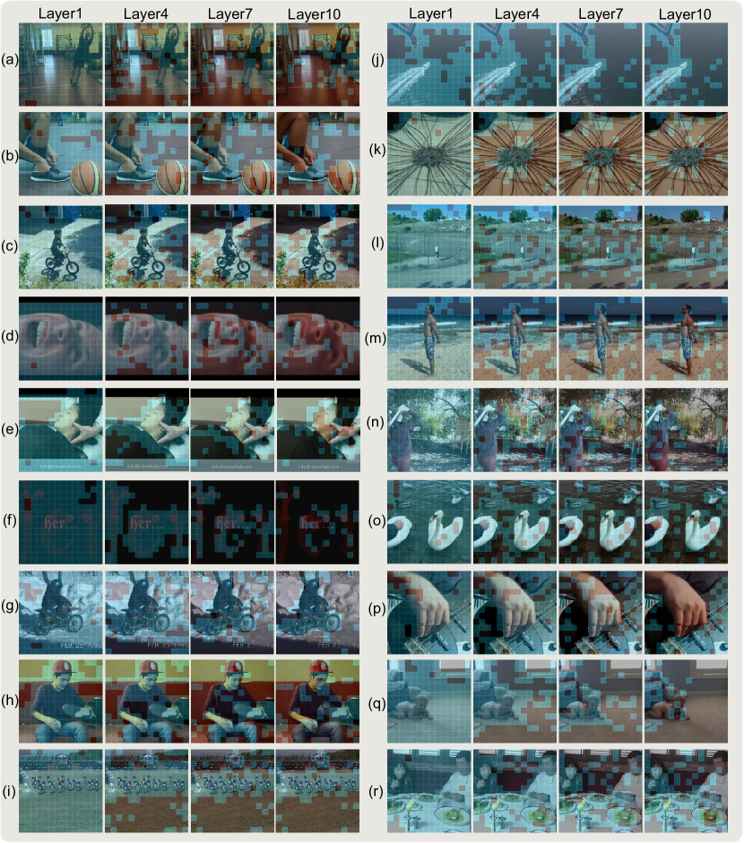
Figure 8: Visualization of activated tokens. We present representative samples from the K400 [9] dataset. Blue patches represent the tokens activated in token dispatcher. Results verify that the token dispatcher has learned to identify informative tokens during fine-tuning. Zoom in for better view.

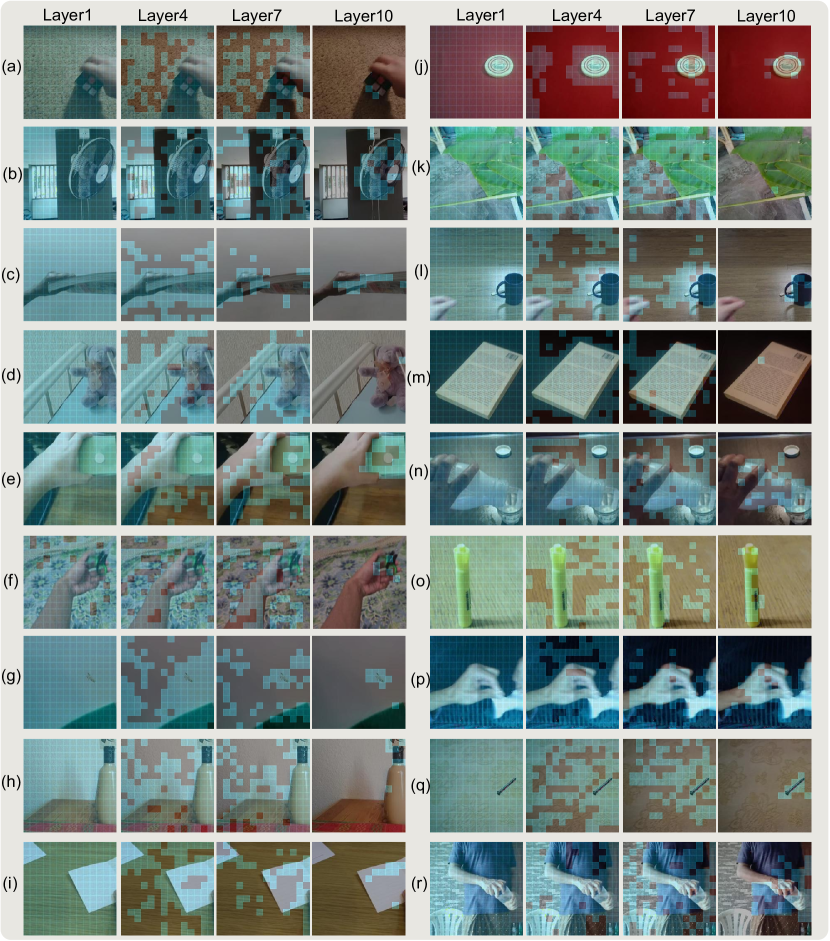
Figure 9: Visualization of activated tokens. We present representative samples from the SSv2 [24] dataset. Blue patches represent the tokens activated in token dispatcher. Results verify that the token dispatcher has learned to identify informative tokens during fine-tuning. Zoom in for better view.

0.A.7 Additional Visualizations of Activated Tokens

We provide more visualizations of activated tokens from samples in K400 [9] and SSv2 [24] in Figure 8 and Figure 9, respectively. Results demonstrate that most activated tokens in higher layers e.g. Layer10 come from the primary objects. This proves that the proposed token dispatcher learns to activate informative tokens.

References

- [1] Ba, J.L., Kiros, J.R., Hinton, G.E.: Layer normalization. arXiv preprint arXiv:1607.06450 (2016)
- [2] Bahng, H., Jahanian, A., Sankaranarayanan, S., Isola, P.: Exploring visual prompts for adapting large-scale models. arXiv preprint arXiv:2203.17274 (2022)
- [3] Bao, H., Dong, L., Wei, F.: Beit: Bert pre-training of image transformers. arxiv 2021. arXiv preprint arXiv:2106.08254
- [4] Bolukbasi, T., Wang, J., Dekel, O., Saligrama, V.: Adaptive neural networks for efficient inference. In: ICML. pp. 527–536. PMLR (2017)
- [5] Bossard, L., Guillaumin, M., Van Gool, L.: Food-101–mining discriminative components with random forests. In: ECCV. pp. 446–461. Springer (2014)
- [6] Caesar, H., Uijlings, J., Ferrari, V.: Coco-stuff: Thing and stuff classes in context. In: CVPR. pp. 1209–1218 (2018)
- [7] Cao, Q., Xu, Z., Chen, Y., Ma, C., Yang, X.: Domain-controlled prompt learning. arXiv preprint arXiv:2310.07730 (2023)
- [8] Cao, Q., Xu, Z., Chen, Y., Ma, C., Yang, X.: Domain prompt learning with quaternion networks. arXiv preprint arXiv:2312.08878 (2023)
- [9] Carreira, J., Zisserman, A.: Quo vadis, action recognition? a new model and the kinetics dataset. In: CVPR. pp. 6299–6308 (2017)
- [10] Chen, S., Ge, C., Tong, Z., Wang, J., Song, Y., Wang, J., Luo, P.: Adaptformer: Adapting vision transformers for scalable visual recognition. NeurIPS 35, 16664–16678 (2022)
- [11] Chen, X., Ding, M., Wang, X., Xin, Y., Mo, S., Wang, Y., Han, S., Luo, P., Zeng, G., Wang, J.: Context autoencoder for self-supervised representation learning. IJCV 132(1), 208–223 (2024)
- [12] Chen, Z., Duan, Y., Wang, W., He, J., Lu, T., Dai, J., Qiao, Y.: Vision transformer adapter for dense predictions. arXiv preprint arXiv:2205.08534 (2022)
- [13] Cimpoi, M., Maji, S., Kokkinos, I., Mohamed, S., Vedaldi, A.: Describing textures in the wild. In: CVPR. pp. 3606–3613 (2014)
- [14] Cubuk, E.D., Zoph, B., Shlens, J., Le, Q.V.: Randaugment: Practical automated data augmentation with a reduced search space. In: CVPR workshops. pp. 702–703 (2020)
- [15] Dehghani, M., Djolonga, J., Mustafa, B., Padlewski, P., Heek, J., Gilmer, J., Steiner, A.P., Caron, M., Geirhos, R., Alabdulmohsin, I., et al.: Scaling vision transformers to 22 billion parameters. In: ICML. pp. 7480–7512. PMLR (2023)
- [16] Deng, J., Dong, W., Socher, R., Li, L.J., Li, K., Fei-Fei, L.: Imagenet: A large-scale hierarchical image database. In: CVPR. pp. 248–255. Ieee (2009)
- [17] Dettmers, T., Pagnoni, A., Holtzman, A., Zettlemoyer, L.: Qlora: Efficient finetuning of quantized llms. arXiv preprint arXiv:2305.14314 (2023)
- [18] Dong, X., Bao, J., Zhang, T., Chen, D., Zhang, W., Yuan, L., Chen, D., Wen, F., Yu, N.: Bootstrapped masked autoencoders for vision bert pretraining. In: ECCV. pp. 247–264. Springer (2022)
- [19] Dosovitskiy, A., Beyer, L., Kolesnikov, A., Weissenborn, D., Zhai, X., Unterthiner, T., Dehghani, M., Minderer, M., Heigold, G., Gelly, S., et al.: An image is worth 16x16 words: Transformers for image recognition at scale. arXiv preprint arXiv:2010.11929 (2020)
- [20] Edalati, A., Tahaei, M., Kobyzev, I., Nia, V.P., Clark, J.J., Rezagholizadeh, M.: Krona: Parameter efficient tuning with kronecker adapter. arXiv preprint arXiv:2212.10650 (2022)
- [21] Gebru, T., Krause, J., Wang, Y., Chen, D., Deng, J., Fei-Fei, L.: Fine-grained car detection for visual census estimation. In: AAAI. vol. 31 (2017)
- [22] Geng, X., Wang, L., Wang, X., Qin, B., Liu, T., Tu, Z.: How does selective mechanism improve self-attention networks? arXiv preprint arXiv:2005.00979 (2020)
- [23] Goodfellow, I.J., Bulatov, Y., Ibarz, J., Arnoud, S., Shet, V.: Multi-digit number recognition from street view imagery using deep convolutional neural networks. arXiv preprint arXiv:1312.6082 (2013)
- [24] Goyal, R., Ebrahimi Kahou, S., Michalski, V., Materzynska, J., Westphal, S., Kim, H., Haenel, V., Fruend, I., Yianilos, P., Mueller-Freitag, M., et al.: The" something something" video database for learning and evaluating visual common sense. In: ICCV. pp. 5842–5850 (2017)
- [25] Han, K., Wang, Y., Chen, H., Chen, X., Guo, J., Liu, Z., Tang, Y., Xiao, A., Xu, C., Xu, Y., et al.: A survey on vision transformer. TPAMI 45(1), 87–110 (2022)
- [26] Han, Y., Han, D., Liu, Z., Wang, Y., Pan, X., Pu, Y., Deng, C., Feng, J., Song, S., Huang, G.: Dynamic perceiver for efficient visual recognition. In: ICCV (2023)
- [27] Han, Y., Huang, G., Song, S., Yang, L., Wang, H., Wang, Y.: Dynamic neural networks: A survey. TPAMI 44(11), 7436–7456 (2021)
- [28] Han, Y., Liu, Z., Yuan, Z., Pu, Y., Wang, C., Song, S., Huang, G.: Latency-aware unified dynamic networks for efficient image recognition. arXiv preprint arXiv:2308.15949 (2023)
- [29] Han, Y., Pu, Y., Lai, Z., Wang, C., Song, S., Cao, J., Huang, W., Deng, C., Huang, G.: Learning to weight samples for dynamic early-exiting networks. In: ECCV. pp. 362–378. Springer (2022)
- [30] Herrmann, C., Bowen, R.S., Zabih, R.: Channel selection using gumbel softmax. In: ECCV. pp. 241–257. Springer (2020)
- [31] Houlsby, N., Giurgiu, A., Jastrzebski, S., Morrone, B., De Laroussilhe, Q., Gesmundo, A., Attariyan, M., Gelly, S.: Parameter-efficient transfer learning for nlp. In: ICML. pp. 2790–2799. PMLR (2019)
- [32] Hu, E.J., Shen, Y., Wallis, P., Allen-Zhu, Z., Li, Y., Wang, S., Wang, L., Chen, W.: Lora: Low-rank adaptation of large language models. arXiv preprint arXiv:2106.09685 (2021)
- [33] Jang, E., Gu, S., Poole, B.: Categorical reparameterization with gumbel-softmax. arXiv preprint arXiv:1611.01144 (2016)
- [34] Jia, M., Tang, L., Chen, B.C., Cardie, C., Belongie, S., Hariharan, B., Lim, S.N.: Visual prompt tuning. In: ECCV. pp. 709–727. Springer (2022)
- [35] Jiang, Z., Mao, C., Huang, Z., Ma, A., Lv, Y., Shen, Y., Zhao, D., Zhou, J.: Res-tuning: A flexible and efficient tuning paradigm via unbinding tuner from backbone. arXiv preprint arXiv:2310.19859 (2023)
- [36] Jie, S., Deng, Z.H.: Convolutional bypasses are better vision transformer adapters. arXiv preprint arXiv:2207.07039 (2022)
- [37] Jie, S., Deng, Z.H.: Fact: Factor-tuning for lightweight adaptation on vision transformer. In: AAAI. vol. 37, pp. 1060–1068 (2023)
- [38] Ju, C., Han, T., Zheng, K., Zhang, Y., Xie, W.: Prompting visual-language models for efficient video understanding. In: ECCV. pp. 105–124. Springer (2022)
- [39] Krizhevsky, A., Hinton, G., et al.: Learning multiple layers of features from tiny images (2009)
- [40] Li, C., Wang, G., Wang, B., Liang, X., Li, Z., Chang, X.: Dynamic slimmable network. In: CVPR. pp. 8607–8617 (2021)
- [41] Li, Y., Song, L., Chen, Y., Li, Z., Zhang, X., Wang, X., Sun, J.: Learning dynamic routing for semantic segmentation. In: CVPR. pp. 8553–8562 (2020)
- [42] Lialin, V., Deshpande, V., Rumshisky, A.: Scaling down to scale up: A guide to parameter-efficient fine-tuning. arXiv preprint arXiv:2303.15647 (2023)
- [43] Lian, D., Zhou, D., Feng, J., Wang, X.: Scaling & shifting your features: A new baseline for efficient model tuning. NeurIPS 35, 109–123 (2022)
- [44] Liang, Y., Ge, C., Tong, Z., Song, Y., Wang, J., Xie, P.: Not all patches are what you need: Expediting vision transformers via token reorganizations. arXiv preprint arXiv:2202.07800 (2022)
- [45] Liu, H., Li, C., Wu, Q., Lee, Y.J.: Visual instruction tuning. NeurIPS 36 (2024)
- [46] Liu, P., Cao, H., Zhao, T.: Gumbel-attention for multi-modal machine translation. arXiv preprint arXiv:2103.08862 (2021)
- [47] Liu, Z., Hu, H., Lin, Y., Yao, Z., Xie, Z., Wei, Y., Ning, J., Cao, Y., Zhang, Z., Dong, L., et al.: Swin transformer v2: Scaling up capacity and resolution. In: CVPR. pp. 12009–12019 (2022)
- [48] Liu, Z., Lin, Y., Cao, Y., Hu, H., Wei, Y., Zhang, Z., Lin, S., Guo, B.: Swin transformer: Hierarchical vision transformer using shifted windows. In: ICCV. pp. 10012–10022 (2021)
- [49] Loshchilov, I., Hutter, F.: Sgdr: Stochastic gradient descent with warm restarts. arXiv preprint arXiv:1608.03983 (2016)
- [50] Loshchilov, I., Hutter, F.: Decoupled weight decay regularization. arXiv preprint arXiv:1711.05101 (2017)
- [51] Maji, S., Rahtu, E., Kannala, J., Blaschko, M., Vedaldi, A.: Fine-grained visual classification of aircraft. arXiv preprint arXiv:1306.5151 (2013)
- [52] Meng, L., Li, H., Chen, B.C., Lan, S., Wu, Z., Jiang, Y.G., Lim, S.N.: Adavit: Adaptive vision transformers for efficient image recognition. In: CVPR. pp. 12309–12318 (2022)
- [53] Nilsback, M.E., Zisserman, A.: Automated flower classification over a large number of classes. In: 2008 Sixth Indian conference on computer vision, graphics & image processing. pp. 722–729. IEEE (2008)
- [54] Pan, J., Lin, Z., Zhu, X., Shao, J., Li, H.: St-adapter: Parameter-efficient image-to-video transfer learning. NeurIPS 35, 26462–26477 (2022)
- [55] Parkhi, O.M., Vedaldi, A., Zisserman, A., Jawahar, C.: Cats and dogs. In: CVPR. pp. 3498–3505. IEEE (2012)
- [56] Pfeiffer, J., Kamath, A., Rücklé, A., Cho, K., Gurevych, I.: Adapterfusion: Non-destructive task composition for transfer learning. arXiv preprint arXiv:2005.00247 (2020)
- [57] Pytorch: Gumbel-softmax. https://pytorch.org/docs/stable/generated/torch.nn.functional.gumbel_softmax.html, pytorch
- [58] Rao, Y., Zhao, W., Liu, B., Lu, J., Zhou, J., Hsieh, C.J.: Dynamicvit: Efficient vision transformers with dynamic token sparsification. NeurIPS 34, 13937–13949 (2021)
- [59] Shazeer, N., Mirhoseini, A., Maziarz, K., Davis, A., Le, Q., Hinton, G., Dean, J.: Outrageously large neural networks: The sparsely-gated mixture-of-experts layer. arXiv preprint arXiv:1701.06538 (2017)
- [60] Song, L., Zhang, S., Liu, S., Li, Z., He, X., Sun, H., Sun, J., Zheng, N.: Dynamic grained encoder for vision transformers. NeurIPS 34, 5770–5783 (2021)
- [61] Teerapittayanon, S., McDanel, B., Kung, H.T.: Branchynet: Fast inference via early exiting from deep neural networks. In: ICPR. pp. 2464–2469. IEEE (2016)
- [62] Touvron, H., Lavril, T., Izacard, G., Martinet, X., Lachaux, M.A., Lacroix, T., Rozière, B., Goyal, N., Hambro, E., Azhar, F., et al.: Llama: Open and efficient foundation language models. arXiv preprint arXiv:2302.13971 (2023)
- [63] Wang, Y., Han, Y., Wang, C., Song, S., Tian, Q., Huang, G.: Computation-efficient deep learning for computer vision: A survey. arXiv preprint arXiv:2308.13998 (2023)
- [64] Wang, Y., Huang, R., Song, S., Huang, Z., Huang, G.: Not all images are worth 16x16 words: Dynamic transformers for efficient image recognition. NeurIPS 34, 11960–11973 (2021)
- [65] Xiao, T., Liu, Y., Zhou, B., Jiang, Y., Sun, J.: Unified perceptual parsing for scene understanding. In: ECCV. pp. 418–434 (2018)
- [66] Xie, E., Wang, W., Yu, Z., Anandkumar, A., Alvarez, J.M., Luo, P.: Segformer: Simple and efficient design for semantic segmentation with transformers. NeurIPS 34, 12077–12090 (2021)
- [67] Yang, B., Bender, G., Le, Q.V., Ngiam, J.: Condconv: Conditionally parameterized convolutions for efficient inference. NeurIPS 32 (2019)
- [68] Yang, L., Han, Y., Chen, X., Song, S., Dai, J., Huang, G.: Resolution adaptive networks for efficient inference. In: CVPR. pp. 2369–2378 (2020)
- [69] Yin, H., Vahdat, A., Alvarez, J., Mallya, A., Kautz, J., Molchanov, P.: Adavit: Adaptive tokens for efficient vision transformer. arXiv preprint arXiv:2112.07658 (2021)
- [70] Yu, B.X., Chang, J., Wang, H., Liu, L., Wang, S., Wang, Z., Lin, J., Xie, L., Li, H., Lin, Z., et al.: Visual tuning. arXiv preprint arXiv:2305.06061 (2023)
- [71] Yu, J., Wang, Z., Vasudevan, V., Yeung, L., Seyedhosseini, M., Wu, Y.: Coca: Contrastive captioners are image-text foundation models. arXiv preprint arXiv:2205.01917 (2022)
- [72] Zaken, E.B., Ravfogel, S., Goldberg, Y.: Bitfit: Simple parameter-efficient fine-tuning for transformer-based masked language-models. arXiv preprint arXiv:2106.10199 (2021)
- [73] Zhai, X., Kolesnikov, A., Houlsby, N., Beyer, L.: Scaling vision transformers. In: CVPR. pp. 12104–12113 (2022)
- [74] Zhai, X., Puigcerver, J., Kolesnikov, A., Ruyssen, P., Riquelme, C., Lucic, M., Djolonga, J., Pinto, A.S., Neumann, M., Dosovitskiy, A., et al.: A large-scale study of representation learning with the visual task adaptation benchmark. arXiv preprint arXiv:1910.04867 (2019)
- [75] Zhang, A., Lipton, Z., Li, M., Smola, A.: Dive into deep learning. arXiv preprint arXiv:2106.11342 (2023)
- [76] Zhang, Y., Zhou, K., Liu, Z.: Neural prompt search. arXiv preprint arXiv:2206.04673 (2022)
- [77] Zhou, B., Zhao, H., Puig, X., Fidler, S., Barriuso, A., Torralba, A.: Scene parsing through ade20k dataset. In: CVPR. pp. 633–641 (2017)
- [78] Zhou, K., Yang, J., Loy, C.C., Liu, Z.: Conditional prompt learning for vision-language models. In: CVPR. pp. 16816–16825 (2022)
- [79] Zhou, K., Yang, J., Loy, C.C., Liu, Z.: Learning to prompt for vision-language models. IJCV 130(9), 2337–2348 (2022)
- [80] Zhu, D., Chen, J., Shen, X., Li, X., Elhoseiny, M.: Minigpt-4: Enhancing vision-language understanding with advanced large language models. arXiv preprint arXiv:2304.10592 (2023)