A tutorial on learning from preferences and choices with Gaussian Processes

Abstract

Preference modelling lies at the intersection of economics, decision theory, machine learning and statistics. By understanding individuals’ preferences and how they make choices, we can build products that closely match their expectations, paving the way for more efficient and personalised applications across a wide range of domains. The objective of this tutorial is to present a cohesive and comprehensive framework for preference learning with Gaussian Processes (GPs), demonstrating how to seamlessly incorporate rationality principles (from economics and decision theory) into the learning process. By suitably tailoring the likelihood function, this framework enables the construction of preference learning models that encompass random utility models, limits of discernment, and scenarios with multiple conflicting utilities for both object- and label-preference. This tutorial builds upon established research while simultaneously introducing some novel GP-based models to address specific gaps in the existing literature.

Keywords: Preference Learning, Object Preference, Label Preference, Choice functions, Gaussian Process, Skew Gaussian Process

Acknowledgments

For the first author, this publication has emanated from research conducted with the financial support of the EU Commission Recovery and Resilience Facility under the Science Foundation Ireland Future Digital Challenge Grant Number 22/NCF/FD/10827. The second author acknowledges support from the SNSF grant number 212164.

1 Introduction

Preference learning (Fürnkranz and Hüllermeier, 2010) aims at learning predictive preference models from data. Unlike regression or classification, where the target variable is a scalar, preference data is in the form of pairwise comparisons, which express a subject’s preference between alternative options.

Depending on the nature of these options, we distinguish two cases: object preferences and label preferences (Fürnkranz and Hüllermeier, 2010). In object preferences, the training data consists of pairwise comparisons among the characteristics or attributes associated with the objects. Example:

• Food preference: The goal is to learn user preferences among various foods by analysing preference data such as ‘I prefer food A over food B’. Implicitly, the user is indicating preferences for specific attributes of the food, such as ingredients and cooking methods. The model learns from these preferences and can then suggest similar dishes to the user based on attributes (ingredients and cooking methods) associated with those dishes.

In label preferences, the training data consists of pairwise comparisons among labels associated with the objects. Example:

• Travel preference: The objective is to gain insights and to predict user preferences for different modes of transportation (in general referred to as labels) such as cars, trains, buses, and bicycles, based on data collected in the form ‘I prefer using a train to go from A to B’. The attributes considered in this context pertain to the user: age, education, and occupation, for example. The aim is to predict transportation modes for new users.

There are also applications where we encounter mixed-type problems, exhibiting characteristics of both label and object preference. We will provide an example in the application section of this tutorial.

There are two main approaches for learning preferences:

1. utility function based;

2. two-argument function based.

Utility function based learning.

This approach exploits a fundamental result in economics (Debreu, 1954): a rational preference relation (that is a binary relation which is asymmetric and negatively transitive) is representable by a utility function (and vice versa), see Section 2.1 for a review. This means that, when presented with various alternatives, a rational subject tends to prefer the option with the highest utility. In preference learning, the utility function is latent (not directly observable) and the objective is to learn this latent function based on the observed subject’s preferences. We can then use the inferred utility function to predict the subject’s preference among options by choosing the alternative with the highest expected utility.

However, in real-world scenarios, individuals often deviate from rationality for different reasons. To account for this behaviour, one modelling approach is to employ random utility models (McFadden, 1974, 1978). These models assume that a subject’s preference is determined by a noisy utility function. The diversity of random utility models arises from different assumptions about the distribution of this noise. Examples of proposed distributions for the noise are Gaussian (Thurstone, 1927) and Gumbel (Luce, 1959). There are other reasons why individuals can deviate from rationality, such as for instance a limit of discernibility (Luce, 1956) between options having close utilities as well as the presence of multiple conflicting utilities (Moulin, 1985). In this tutorial, we will review and implement various learning models designed to address the aforementioned source of irrationality in preferences.

Finally, we must mention that in many applications we do not observe preferences, but only the choices of a subject, that is the options the subject has selected among the given alternatives. Therefore, we must also be able to learn from choice data. Under some rationality assumptions in the way individuals make choices, it is still possible to learn the underlying utility function(s), which determines the subject’s choices. In economics, stating the conditions of rationality that make this possible is referred to as the revealed preference theory (Samuelson, 1938).

Preference learning with two-argument functions.

This approach directly learns a preference relation as a two-argument function. Expressing preferences through two-argument functions has been studied in economics to model non-transitive preferences, see, for instance, Shafer (1974); Fishburn (1988). In machine learning, this is the predominant (Fürnkranz and Hüllermeier, 2010) method for preference learning, because it allows the practitioner to frame the problem as a classification task. This approach (van Cranenburgh et al., 2022) works without imposing specific model assumptions, relying solely on a data-driven methodology. However, the effectiveness of this method in learning properties like (quasi-)transitivity from data hinges on a substantial amount of data, making it particularly well-suited for applications with large datasets (Wong and Farooq, 2020; Sifringer et al., 2020; Lederrey et al., 2021).

1.1 Objective of this tutorial

Our goal is to establish a modelling framework for preference learning that can integrate utility-based models, random utility models, limits of discernibility, and scenarios involving multiple conflicting utilities. We aim to achieve this by introducing a Gaussian Process (GP) based approach for both object and label preference learning based on the existing literature (Chu and Ghahramani, 2005; Houlsby et al., 2011; Lun Chau et al., 2022; Nguyen et al., 2021; Benavoli et al., 2023a), as well as developing novel GP-based models to address specific gaps in this literature. The presented models come with a Python library prefGP (Benavoli and Azzimonti, 2024), we have developed for this tutorial, enabling practitioners to seamlessly apply these models to their data, facilitating comparison and analysis.

Why Gaussian processes?

First, in comparison to traditional statistics literature on preference learning, GPs enable us to move beyond the assumption of a linear utility function in the covariates. In contrast to the machine learning literature, GPs allow us to directly model the utility function without the need to parameterise it, for instance, through a Neural Network. This simplifies both the modelling treatment and the model inference process. Second, for several preference models, GPs offer an efficient (rejection-free) method to sample from the posterior. Third, we seek a model that can automatically adjust its own complexity to the data – a crucial aspect in preference learning for achieving ‘exact interpolation’, essential for modelling the utility function of a rational subject. Fourth, a kernel-based approach gives greater versatility in handling various types of data; for instance, it allows the definition of kernels on images and graphs as well as defining specific preference kernels (Houlsby et al., 2011; Lomeli et al., 2019; Lun Chau et al., 2022). Finally, GPs provide an estimate of their own uncertainty, a valuable aspect in decision-making. For example, it can be employed for active preference learning (Eric et al., 2007; Zoghi et al., 2014) and Preferential Bayesian optimisation (Shahriari et al., 2015; González et al., 2017; Siivola et al., 2021; Benavoli et al., 2021c; Nguyen et al., 2021; Benavoli et al., 2023b; Xu et al., 2024; Takeno et al., 2023).

It is important to note that our modelling approach involves specifying different likelihoods, while using the same prior, a GP. Hence, this tutorial is also valuable for practitioners who aim to model preferences using the same likelihoods (cost functions) while employing alternative machine learning models to fit the utility.

We will present and derive 9 models to learn from preference and choice data:

Model 3.1:

Consistent Preferences.

Model 3.2.1:

Just Noticeable Difference.

Model 3.2.1:

Probit for Erroneous Preferences.

Model 3.2.3:

Preferences with Gaussian noise error.

Model 3.3:

Probit for Erroneous preferences as a classification problem.

Model 4.1:

Thurstonian model for label preferences.

Model 4.2:

Plackett-Luce model for label ordering data.

Model 4.3:

Paired comparison for label preferences.

Model 5.2:

Rational and Pseudo-rational models for choice data.

A drawback of GPs is their computational complexity, $\mathcal{O}(N^{3})$ time complexity and $\mathcal{O}(N^{2})$ memory complexity, where $N$ is a size of the training data. However, there are a number of well established ways to scale up GPs (to $\mathcal{O}(N)$) that can be easily applied to the above models by using inducing points (Quiñonero-Candela and Rasmussen, 2005; Snelson and Ghahramani, 2006), in combination with variational inference (Titsias, 2009; Hensman et al., 2013; Hernandez-Lobato and Hernandez-Lobato, 2016) or other well-established approaches (Bauer et al., 2016; Schuerch et al., 2020, 2023).

1.2 Literature overview

The literature in preference learning is vast. The following books provide an overview of the main models and challenges: Marden (1996); Train (2009); Fürnkranz and Hüllermeier (2010); Alvo and Philip (2014).

The most popular Random Utility Models (RUMs) for preference learning are variants of the Bradley-Terry model (Bradley and Terry, 1952), Babington-Smith model (Smith, 1950; Mallows, 1957), and Thurstone-Mosteller model (Thurstone, 1927; Mosteller and Nogee, 1951). These models assume either a Gumbel noise, resulting in a logit likelihood, or a Gaussian noise, giving rise to a probit likelihood. Traditionally, these models have been designed for label-preference and they are fitted via maximum likelihood estimation using different methods (Hunter, 2004; Shah et al., 2015; Maystre and Grossglauser, 2015; Vojnovic and Yun, 2016; Ragain and Ugander, 2016; Agarwal et al., 2018). Bayesian models and inference are instead proposed in Guiver and Snelson (2009); Caron and Doucet (2012); Azari et al. (2012).

The extensions of the above RUMs to include covariates are known as multinomial logit models (McFadden, 1974, 1978) and multinomial probit models. The main difference between these two models lies in their treatment of the noise. The first model assumes independent noises, whereas the second model assumes dependent noises, specifically in the form of Gaussian correlated noises. Apollo (Hess and Palma, 2019) and mlogit (Croissant, 2020) are R packages which allow to fit multinomial logit/probit models using maximum likelihood. Biogeme (Bierlaire, 2018), Pylogit (Brathwaite and Walker, 2018), torch-choice (Du et al., 2023) are similar Python-based libraries.

These models have been unified within the framework of generalised linear models (Critchlow and Fligner, 1991) and, then extended to support vector machines (Evgeniou et al., 2005; Maldonado et al., 2015).

A Bayesian nonparametric approach based on Gaussian Processes for preference learning was firstly proposed by Chu and Ghahramani (2005) and by Houlsby et al. (2011) for both object- and label-preference with a probit likelihood. This approach offers two advantages: a nonlinear utility in the covariates and the representation of uncertainty through the posterior. Since the posterior is not Gaussian, Chu and Ghahramani (2005) proposed the Laplace’s approximation for inference. Other approximations were considered by Houlsby et al. (2011). Recently, Benavoli et al. (2021b, a) showed that the posterior is a Skew-GP and employed a rejection-free procedure to efficiently sample from the posterior.

Apart from random utilities, there are other reasons why individuals can deviate from rationality, such as for instance a limit of discernibility (Luce, 1956) between options having close utilities. Furthermore, deviations may arise in cases where the subject’s preferences are determined by multiple utility functions. Rationalising preferences and, more in general, choices based on multiple utilities has been extensively studied in economics (Moulin, 1985; Eliaz and Ok, 2006). An extension of logit-based RUM to deal with multiple utilities has been proposed in Benson et al. (2018). A more general model derived to learn choice functions via multiple utilities (through a Pareto embedding) was derived in Pfannschmidt and Hüllermeier (2020), using a hinge-loss and a neural network based model. A GP and probit version of the above model was formulated in Benavoli et al. (2023a).

The non utility-based approach to preference learning aims to directly learn a two-argument function. This problem can be formulated as an augmented binary classification problem or constrained classification (SVM), see, e.g., Cohen et al. (1997); Herbrich et al. (1998); Aiolli and Sperduti (2004); Har-Peled et al. (2002); Fiechter and Rogers (2000); Hüllermeier et al. (2008); Fürnkranz and Hüllermeier (2010). For Gaussian Processes, Houlsby et al. (2011) derived the theoretical link between the GP-based probit model for rational preference learning based on RUM and the two-argument function. Indeed, a GP prior on the latent utility $u({\bf x}_{i})$ induces a GP prior on the two-argument function $q({\bf x}_{i},{\bf x}_{j})=u({\bf x}_{i})-u({\bf x}_{j})$ by linearity, see Section 3.3 for more. This allowed Houlsby et al. (2011) to derive the so called preference kernel. Pahikkala et al. (2010) instead, using a feature map view, derived the kernel of a two-argument function which allows one to model preferences satisfying asymmetry but not transitivity in general. This kernel is known as intransitive preference kernel. A preference-learning model which employs a GP prior on $q$ based on this intransitive kernel was proposed by Lun Chau et al. (2022).

In this tutorial, we will not cover the discussion of techniques for deducing the consensus preference within a group of subjects or about aggregation methods. It is worth noting that certain methods we will introduce in this tutorial may be applicable to such scenarios, such as interpreting multiple utilities as arising from distinct subjects (multi-self). Nonetheless, it is important to stress that the aggregation problem has been extensively investigated in the literature, see, for instance, Arrow (1963); Fligner and Verducci (1990); Meilă et al. (2007); Negahban et al. (2012); Azari Soufiani et al. (2013); Caragiannis et al. (2016). A related problem to aggregation is ranking and learning from ranking data, in this case the input-data is a complete or partial ordering of labels. For example, a partial ordering appears when users are asked to order (rank) their top-10 movies or the result of a web-search. A linear RUM used to learn from ordering data is the Plackett-Luce model (Luce, 1959; Plackett, 1975). There have been many models developed for recommendation systems (Ricci et al., 2015), for instance based on neural networks (“learning to rank”, Burges et al. (2005); Burges (2010)). A GP nonlinear extension of Plackett-Luce was derived by Nguyen et al. (2021) and we will discuss it in this tutorial.

It is important to highlight that preference learning is accompanied by its own computational challenges. The potential number of preferences among $n$ objects is $n(n-1)/2$ and it can become large for big datasets. In the case of choice data, computational complexity can increase factorially based on the choice-set’s size, depending on the specific problem and the subject’s decisions. In label-preference, the number of utilities is equal to the number of labels, leading to large number of utilities in many applications. This implies that computational considerations must also be taken into account when choosing a model. Related to this, an important area of research pertains to the elicitation of preferences (Boutilier et al., 2006; Boutilier, 2013; Bourdache et al., 2019; Adam and Destercke, 2021b, a).

Finally, in this tutorial, we will not cover preference-based reinforcement learning, a framework that enables learning from non-numerical feedback in sequential domains. Compared to standard reinforcement learning, preference-based learning offers the advantage of defining feedback that is independent of arbitrary reward choices/shaping/engineering (Wirth et al., 2017). This approach has recently found applications in training large language models (Christiano et al., 2017; Stiennon et al., 2020; Ouyang et al., 2022; Rafailov et al., 2023). In this dynamic context, an essential consideration involves extending consistency principles of preference over time (Troffaes and Goldstein, 2013).

1.3 Tutorial organisation

Section 2 introduces the mathematical objects and concepts that will be use in the rest of the tutorial. Section 3 will focus on object preference. In particular, a model to learn from consistent preference is introduced in Section 3.1. We will then modify this model to account for possible sources of irrationality: limit of discernibility in Section 3.2.1; additive Gaussian noise in Section 3.2.3 and multiple conflicting utilities in Section 3.2.4. All the above models aim to learn the utility function of the subject. Section 3.3 delves into directly learning the preference relation as a two-argument function. We will then move to label-preference in Section 4 discussing two RUMs based on Gaussian noise in Section 4.1 and Gumbel noise in Section 4.2. We then present a model for label-preference learning based on pairwise comparisons in Section 4.3. We will then move to choice functions in Section 5 introducing two models in Section 5.2. Section 6 will discuss applications. Finally, section 7 concludes the tutorial.

2 Preliminaries

In this section, we introduce some of the mathematical objects and concepts that we will use in the next sections. We start by defining preferences and utility functions. We will then move to Gaussian Processes, which is the statistical model we will use to learn from preference data.

2.1 Preferences and Utilities

Consider a finite set $\mathcal{X}$ and a binary relation $R$ on $\mathcal{X}$ expressed by a subject. $R$ is a subset of $\mathcal{X}\times\mathcal{X}$. For any two elements of $\mathcal{X}$, the statement $(x,y)\in R$, denoted by $xRy$, tells us that, according to the subject, ‘x is R-related to y’ in some way.

The following is a list of common properties of binary relations.

• Reflexive: $\forall x\in\mathcal{X}$ $xRx$;

• Irreflexive: $\forall x\in\mathcal{X}$ $\neg xRx$, where $\neg$ stands for logical negation;

• Symmetric: $\forall x,y\in\mathcal{X}$ if $xRy$ then $yRx$;

• Asymmetric: $\forall x,y\in\mathcal{X}$ if $xRy$ then not $yRx$;

• Negatively transitive: if $xRy$ then for any other element $z\in\mathcal{X}$ either $xRz$ or $zRy$ or both.

• Transitive: $\forall x,y,z\in\mathcal{X}$ if $xRy$ and $yRz$ then $xRz$.

• Acyclicity: If, for any finite number $n$, $x_{1}Rx_{2}$, $x_{2}Rx_{3}$, $\dots$, $x_{n-1}Rx_{n}$ then $x_{n}\neq x_{1}$.

• Completeness: $\forall x,y\in\mathcal{X}$ either $xRy$ or $yRx$ or both.

Preferences are particular types of relations and they are for instance used to model a consumer. Given two objects, Alice (the subject/consumer) may say that “$x$ is better than $y$” and, in this case, we write the relation $xRy$ as $x\succ y$, read as $x$ is strictly preferred to $y$.

Definition 1

A strict preference is a binary relation, denoted by $\succ$, which is asymmetric and negatively transitive.

The asymmetry implies that the subject cannot say that $x$ is better than $y$ and also that $y$ is better than $x$. The property negatively transitivity is clearer when formulated as “if $x\nsucc z$ and $z\nsucc y$ then $x\nsucc y$”, which means that if $x$ is not better than $z$ and $z$ not better than $y$ then $x$ is not better than $y$. A strict preference relation is said to be consistent – Alice is rational – when it satisfies the above two properties.

Proposition 2

(Kreps et al. (1990, Prop. 2.1)) Any strict preference is irreflexive, transitive and acyclic.

We point the reader to Kreps et al. (1990, Ch. 2) for the proofs of the results in this section. From $\succ$, we can define two new relations called weak preference and, respectively, indifference.

Definition 3

For each $x,y\in\mathcal{X}$, $x\succeq y$ (read as $x$ weakly preferred to $y$), if it is not the case that $y\succ x$. For each $x,y\in\mathcal{X}$, $x\sim y$ (read as $x$ is indifferent to $y$), if it is not the case that either $x\succ y$ or $y\succ x$.

Proposition 4

(Kreps et al. (1990, Prop. 2.2)) The above weak preference relation is complete and transitive. The above indifference relation is reflexive, symmetric and transitive.

It is worth noticing that:

Proposition 5

1. $\succ$ is asymmetric iff $\succeq$ is complete;

2. $\succ$ is negatively transitive iff $\succeq$ is transitive.

2.1.1 Representation via utility function

Strict preferences can be represented by a value function. We refer to a value function that represents preferences as a utility function.

Definition 6

For any set $\mathcal{X}$ and preference relation $\succ$ (resp. $\succeq$) on $\mathcal{X}$, the function $u:\mathcal{X}\rightarrow\mathbb{R}$ represents $\succ$ (resp. $\succeq$) if

$$x\succ y~{}~{}\textit{ iff }~{}~{}u(x)>u(y)~{}~{}~{}~{}\textit{(resp. $x\succeq y~{}~{}\textit{ iff }~{}~{}u(x)\geq u(y)$)}~{}~{}\forall x,y\in\mathcal{X}$$

We say that $u$ is a utility function for $\succ$ (resp. $\succeq$).

This means that, when presented with various alternatives, a rational subject tends to prefer the option with the highest utility. When does $\succ$ admit a utility function representation? If $\mathcal{X}$ is finite, $\succ$ admits a utility function representation iff it is asymmetric and negatively transitive (Kreps et al., 1990, Ch. 2). However, this representation is not unique. Indeed, utility functions are invariant under increasing transformations. We can define a new utility function $g(u(x))$ for any increasing function $g$, that is, $\forall x,y\in\mathcal{X}$ we have

$$x\succ y~{}\textit{ iff }~{}u(x)>u(y)~{}\textit{ iff }~{}g(u(x))>g(u(y)).$$

So $u$ and $g(u)$ represent the same strict preference relation. What this means is that, we treat utility functions as ordinal rather than cardinal. That is, only the relative ranking of two items is important, not the magnitude of their utility difference. The reader should keep this in mind for the next sections.

2.2 Gaussian process

As we will see in the next sections, there are two main ways to learn from preference data. We can learn either the preference-relation (the binary-relation) or the utility function that represents it. Since a binary-relation is a function that assigns truth values (true or false) to two elements of $\mathcal{X}$, in both cases learning preferences reduces to learning a function.

An elegant way to learn functions is by defining a prior probability over functions and then compute the posterior distribution given the data. Gaussian Processes (GPs) are prior over functions (O’Hagan, 1978; Rasmussen and Williams, 2006), that have attractive advantages over parametric (including neural networks) models. They are nonparametric, meaning that their complexity automatically grows as more data are observed and, therefore, they have the ability to exactly ‘interpolate’ the data, which is important to model consistent preference relations.

They have a small number of tunable hyperparameters (and so they can be trained on small datasets), and naturally provide an uncertainty measure on their predictions. Moreover, by being kernel based, they provide a framework to learn utility functions defined on any domain $\mathcal{X}$ on which we can define a kernel function.

To define a prior over a function $f:\mathcal{X}\rightarrow\mathbb{R}$, a GP assumes that, for every $n$, $p(f({\bf x}_{1}),\dots,f({\bf x}_{n}))$ is jointly Gaussian, with mean $[\mu({\bf x}_{1}),\dots,\mu({\bf x}_{n})]$ and covariance
$Cov(f({\bf x}_{i}),f({\bf x}_{j}))=k({\bf x}_{i},{\bf x}_{j})$, for $i,j=1,\ldots,n$. $\mu({\bf x})$ and $k({\bf x},{\bf x}^{\prime})$ are the mean function and, respectively, the (positive definite) kernel function of the GP. A GP is usually parametrised with a zero mean function $\mu({\bf x})=0$ and a covariance kernel $k_{\bm{\theta}}({\bf x},{\bf x}^{\prime})$ which depends on hyperparameters $\bm{\theta}\in\Theta$. A typical example is the automatic relevance determination (ARD) Square-Exponential (SE) kernel on $\mathbb{R}^{c}$, $c\in\mathbb{N}$. For ${\bf x},{\bf x}^{\prime}\in\mathbb{R}^{c}$ it is defined as

$$k_{\bm{\theta}}({\bf x},{\bf x}^{\prime})=\displaystyle{\sigma_{k}^{2}\,\exp\left(-\sum_{i=1}^{c}\frac{(x_{i}-x_{i}^{\prime})^{2}}{2\ell_{i}^{2}}\right)},$$ (1)

where $\bm{\theta}=[\ell_{1},\dots,\ell_{c},\sigma_{k}^{2}]$ includes the lengthscale hyperparameters $\ell_{i}>0$ (one for each dimension) and the scale parameter $\sigma_{k}^{2}$. GPs have a natural Bayesian interpretation that makes them ideal for regression problems. If we assume that the observed values are the sum of a true function evaluated at some inputs plus Gaussian noise, i.e. $y_{i}=f({\bf x}_{i})+\varepsilon_{i}$ with $\varepsilon_{i}\sim N(0,\sigma^{2})$ for $i=1,\ldots,n$, then we can analytically compute the posterior distribution of $f$. We can write the observation model more compactly as the likelihood

$$p(y_{1},\ldots,y_{n}|f({\bf x}_{1}),\ldots,f({\bf x}_{n}))=N(\mathbf{y}_{n}|{f}(X),\sigma^{2}I_{n}),$$

where $\mathbf{y}_{n}=[y_{1},\dots,y_{n}]^{\top}$, $X=[{\bf x}_{1},\dots,{\bf x}_{n}]^{\top}$ and $I_{n}$ is the identity matrix of dimension $n$. In particular, the predictive posterior at a new test point ${\bf x}^{*}\in\mathcal{X}$ is $GP(\mu_{p},k_{p})$, with mean and covariance kernel:

$$\mu_{p}({\bf x}^{*}) =K_{\bm{\theta}}({\bf x}^{*},X)(K_{\bm{\theta}}(X,X)+\sigma^{2}I_{n})^{-1}\mathbf{y}_{n}$$ (2)

$$k_{p}({\bf x}^{*},{\bf x}^{*}) =K_{\bm{\theta}}({\bf x}^{*},{\bf x}^{*})-K_{\bm{\theta}}({\bf x}^{*},X)(K_{\bm{\theta}}(X,X)+\sigma^{2}I_{n})^{-1}K_{\bm{\theta}}(X,{\bf x}^{*}),$$ (3)

where $K_{\bm{\theta}}(X,X)$ is a matrix whose ij-th element is defined as $(K_{\bm{\theta}}(X,X))_{ij}=k_{\bm{\theta}}({\bf x}_{i},{\bf x}_{j})$ (similar for $K_{\bm{\theta}}({\bf x}^{*},X)$). Note that, the variance of the likelihood $\sigma^{2}$ is also considered to be a hyperparameter. The hyperparameters $\bm{\theta},\sigma^{2}$ are commonly estimated by maximising the marginal likelihood:

$$p(({\bf x}_{i},y_{i})_{i=1}^{n}|\bm{\theta},\sigma^{2})=N(\mathbf{y}_{n},K_{\bm{\theta}}(X,X)+\sigma^{2}I_{n}).$$

In tasks with likelihoods different from the Gaussian, the posterior is not a GP. For Probit (classification/preference learning) and Skew-Normal likelihoods, the posterior is a Skew GP (Benavoli et al., 2021a). We point the reader to Appendix B for details. For other likelihoods, in general the posterior does not have a closed-form and is approximated with a GP using three main approaches: (i) Laplace’s approximation (LP) (MacKay, 1996; Williams and Barber, 1998); (ii) Expectation Propagation (EP) (Minka, 2001); (iii) Kullback-Leibler divergence (KL) minimization (Opper and Archambeau, 2009), comprising Variational Bounding (VB) (Gibbs and MacKay, 2000) as a particular case.

3 Learning from object preferences

As we discussed in Section 1, there are two types of preferences: preferences on objects and preferences on labels. In this section, we will focus on the first type.

Therefore, our aim is to learn Alice’s preference relation $\succ$ on a set of objects $\mathcal{X}$ from a finite set of examples, the training set. We represent each object by the feature vector ${\bf x}\in\mathbb{R}^{c}$ of its characteristics and denote the objects in $\mathcal{X}$ as ${\bf x}_{i}\in\mathcal{X}$. We will explore different variants of this problem that allow for some deviations from rationality in the subject, which can help address practical challenges when comparing objects.

3.1 Learning consistent preferences

First, we will focus on learning consistent (rational) preferences. Consider a vector of objects $X=[{\bf x}_{1},{\bf x}_{2},\dots,{\bf x}_{r}]^{\top}$ such that ${\bf x}_{i}\in\mathbb{R}^{c}$ for all $i=1,\dots,r$, we denote the training set of $m$ pairwise preferences as

$$\mathcal{D}_{m}=\{{\bf x}_{i_{s}}\succ{\bf x}_{j_{s}}:~{}~{}s=1,\dots,m\},$$

where ${\bf x}_{i_{s}}\succ{\bf x}_{j_{s}}$ is the s-th pairwise preference, with ${\bf x}_{i_{s}}\neq{\bf x}_{j_{s}}$, ${\bf x}_{i_{s}},{\bf x}_{j_{s}}\in X$, $i_{s},j_{s}\in\{1,2,\dots,r\}$ for each $s=1,\dots,m$. As discussed in Section 2.1, whenever Alice’s preference relation is consistent, that is, it satisfies asymmetry and negative transitivity, we can assume that Alice has in mind a function $u$ that attaches to each alternative a numerical value; the higher the value, the better Alice likes the alternative. We can then rewrite $\mathcal{D}_{m}$ as $\mathcal{D}_{m}=\{u({\bf x}_{i_{s}})-u({\bf x}_{j_{s}})>0:~{}~{}s=1,\dots,m\}$. Preference learning is then the task of learning the function $u$ from $\mathcal{D}_{m}$.

Example 1 (Thermal comfort)

To introduce the concepts, we make use of a simple running example: learning Alice’s preferred home temperature. We present Alice with pairs of temperatures (in Celsius) and ask her preferred value. Imagine Alice’s utility is as depicted in Figure 1, namely, she has three locally most preferred temperature depending on her activity in the house (home-fitness, working, relaxing).

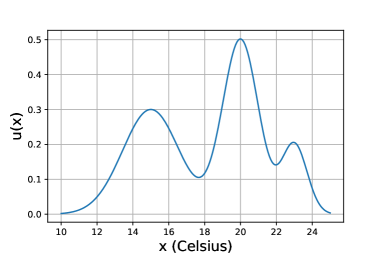
Figure 1: Alice’s utility for home temperature.

In order to infer her utility function, we consider the set of temperatures (objects) $\mathcal{X}=\{10,11,12,\dots,25\}$ and asks her preferences for $19$ pairs of temperatures. This results in the dataset:

$$\mathcal{D}_{19}= \{12\succ 10,13\succ 25,14\succ 13,15\succ 22,15\succ 23,16\succ 11,19\succ 15,19\succ 21,19\succ 22,$$

$$19\succ 24,20\succ 10,20\succ 14,20\succ 21,20\succ 24,20\succ 25,21\succ 13,21\succ 25,23\succ 25,24\succ 25\}.$$ (4)

We aim to learn Alice’s utility function for home-temperature from $\mathcal{D}_{19}$ and predict her preferences for any other pairs of temperatures.

To this purpose, it is useful to represent the statements in $\mathcal{D}_{m}$ in matrix form. Define $u(X)=[u({\bf x}_{1}),u({\bf x}_{2}),\dots,u({\bf x}_{r})]^{\top}$ and $W$ is a $m\times r$ matrix whose s-th row is all zero apart from $W_{i_{s}}=1,W_{j_{s}}=-1$. Then we can equivalently write the preference statements using a matrix representation $\mathcal{D}_{m}=\{Wu(X)>0\}$.

Example 2

For the dataset $\mathcal{D}_{19}$ in Example 1, the constraints $Wu(X)>0$ are as follows:

$$\setcounter{MaxMatrixCols}{15}\begin{bmatrix}[r]-1&0&1&0&0&0&0&0&0&0&0&0&0&0&0\\ 0&0&0&1&0&0&0&0&0&0&0&0&0&0&-1\\ 0&0&0&-1&1&0&0&0&0&0&0&0&0&0&0\\ 0&0&0&0&0&1&0&0&0&0&0&-1&0&0&0\\ 0&0&0&0&0&1&0&0&0&0&0&0&-1&0&0\\ 0&-1&0&0&0&0&1&0&0&0&0&0&0&0&0\\ 0&0&0&0&0&-1&0&0&1&0&0&0&0&0&0\\ 0&0&0&0&0&0&0&0&1&0&-1&0&0&0&0\\ 0&0&0&0&0&0&0&0&1&0&0&-1&0&0&0\\ 0&0&0&0&0&0&0&0&1&0&0&0&0&-1&0\\ -1&0&0&0&0&0&0&0&0&1&0&0&0&0&0\\ 0&0&0&0&-1&0&0&0&0&1&0&0&0&0&0\\ 0&0&0&0&0&0&0&0&0&1&-1&0&0&0&0\\ 0&0&0&0&0&0&0&0&0&1&0&0&0&-1&0\\ 0&0&0&0&0&0&0&0&0&1&0&0&0&0&-1\\ 0&0&0&-1&0&0&0&0&0&0&1&0&0&0&0\\ 0&0&0&0&0&0&0&0&0&0&1&0&0&0&-1\\ 0&0&0&0&0&0&0&0&0&0&0&0&1&0&-1\\ 0&0&0&0&0&0&0&0&0&0&0&0&0&1&-1\\ \end{bmatrix}\begin{bmatrix}u(10)\\ u(11)\\ u(12)\\ u(13)\\ u(14)\\ u(15)\\ u(16)\\ u(18)\\ u(19)\\ u(20)\\ u(21)\\ u(22)\\ u(23)\\ u(24)\\ u(25)\\ \end{bmatrix}>0.$$

It can be noticed that the 8-th column is all zero, since the temperature 18 is not included in $\mathcal{D}_{19}$. What can we infer about Alice’s preference $20\stackrel{{\scriptstyle?}}{{\succ}}18$ from the data in $\mathcal{D}_{19}$? We will answer this question in Example 4.

We can express the statements in $Wu(X)>0$ as a likelihood:

$$p(\mathcal{D}_{m}|u(X))=\prod_{s=1}^{m}I_{\{u({\bf x}_{i_{s}})-u({\bf x}_{j_{s}})>0\}}(u(X))=I_{\{Wu(X)>0\}}(u(X)),$$ (5)

where $I_{A}(x)$ is the indicator function: it is equal to one when $x\in A$, equivalently when $x$ satisfies the statement $A$, and zero otherwise.

In GP-based preference learning, we assume a GP prior over $u(X)$, the likelihood (5) and then compute the posterior distribution for $u(X)$.

Lemma 7

Assuming $p(u)=\mathrm{GP}(u;0,k_{\bm{\theta}})$ with a strictly positive definite kernel $k_{\bm{\theta}}$, the posterior is equal to:

$$p(u(X)|\mathcal{D}_{m})=TN_{\{Wu(X)>0\}}(u(X);\mathbf{0},K_{\bm{\theta}}(X,X)),$$ (6)

where the term on the right hand side denotes a multivariate normal distribution with zero mean and covariance matrix $K_{\bm{\theta}}(X,X)$ truncated in $\{u(X)\in\mathbb{R}^{r}:Wu(X)>0\}$. The posterior is well-defined provided that $\succ$ satisfies asymmetry and negative transitivity.

Remark 8

Since the set $\{u(X)\in\mathbb{R}^{r}:Wu(X)\geq 0\}\backslash\{u(X)\in\mathbb{R}^{r}:Wu(X)>0\}$ has zero measure with respect to the Gaussian distribution $N(u(X);\mathbf{0},K_{\bm{\theta}}(X,X))$, we can equivalently write the posterior as:

$$p(u(X)|\mathcal{D}_{m})=TN_{\{Wu(X)\geq 0\}}(u(X);\mathbf{0},K_{\bm{\theta}}(X,X)).$$ (7)

Observe that, this is different from assuming that the underlying preference relation is weak (instead of strict). Indeed we cannot learn a weak preference relation using a GP-based model. To see that, consider for instance the training set $\mathcal{D}_{2}=\{u({\bf x}_{1})-u({\bf x}_{2})\geq 0,u({\bf x}_{2})-u({\bf x}_{1})\geq 0\}$ (which violates asymmetry), this implies that $u({\bf x}_{1})=u({\bf x}_{2})$ but the probability of the evidence:

$$p(\mathcal{D}_{2})=\int I_{\{u({\bf x}_{1})=u({\bf x}_{2})\}}(u(X))N(u(X);\mathbf{0},K_{\bm{\theta}}(X,X))du(X)=0,$$

and, therefore, the posterior cannot be defined via Bayes’ rule (the denominator is zero).

Given the posterior (7), we can compute the predictive posterior as follows.

Proposition 9

The posterior predictive distribution for $u(X^{*})$ given the test-points $X^{*}=[{\bf x}_{1},\dots,{\bf x}_{p}]$ is

$$p(u(X^{*})|\mathcal{D}_{m})=\int p(u(X^{*})|u(X))\;TN_{\{Wu(X)\geq 0\}}(u(X);\mathbf{0},K_{\bm{\theta}}(X,X))du(X),$$ (8)

where

$$p(u(X^{*})|u(X))=N(u(X^{*}); ~{}K_{\bm{\theta}}(X^{*},X)K^{-1}_{\bm{\theta}}(X,X)u(X),$$ (9)

$$~{}K_{\bm{\theta}}(X^{*},X^{*})-K_{\bm{\theta}}(X^{*},X)K^{-1}_{\bm{\theta}}(X,X)K_{\bm{\theta}}(X,X^{*})).$$

The computation of posterior and predictive posterior expectations is nontrivial due to the analytically intractable normalising constant of the truncated normal distribution. However, we can easily approximate the posterior by Monte Carlo sampling. Efficient sampling of truncated multivariate normal distributions under linear inequality constraints can be performed by using Gibbs sampling (Kotecha and Djuric, 1999; Taylor and Benjamini, 2016) linear elliptical slice sampler (lin-ess) (Gessner et al., 2020), minimax tilting method accept-reject sampler (Botev, 2017) and Hamiltonian Monte-Carlo (Pakman and Paninski, 2014).

We will use lin-ess because it only needs the Cholesky factorisation of $K_{\bm{\theta}}(X,X)$, details can be found in Gessner et al. (2020). We provide a visual illustration of this sampling procedure in the next example.

Example 3 (Lin-ess)

Assume for simplicity we have only one preference in the dataset $\mathcal{D}=\{u({\bf x}_{2})-u({\bf x}_{1})\geq 0\}$. The above constraint on $u$ defines a half-space region depicted in Figure 2 (shaded blue region). Let $s_{0}$ be the sample of the vector $[u({\bf x}_{1}),u({\bf x}_{2})]^{\top}$ accepted at the previous step, that is satisfying the constraint. Lin-ess works as follows: (i) sample a new point from the GP (Multivariate-Normal) prior, which in this case is equal to:

$$\nu\sim N\left(\begin{bmatrix}0\\ 0\\ \end{bmatrix},\begin{bmatrix}k_{\bm{\theta}}({\bf x}_{1},{\bf x}_{1})&k_{\bm{\theta}}({\bf x}_{1},{\bf x}_{2})\\ k_{\bm{\theta}}({\bf x}_{2},{\bf x}_{1})&k_{\bm{\theta}}({\bf x}_{2},{\bf x}_{2})\\ \end{bmatrix}\right).$$

(ii) define the ellipse $\{\cos(\phi)s_{0}+\sin(\phi)\nu:~{}\phi\in[0,2\pi)\}$ shown in Figure 2. (iii) calculate analytically the interval $[\phi_{min},\phi_{max}]$ including the values of $\phi$ corresponding to the slice of the ellipse inside the constraint region. (iv) finally generate a new sample $s_{1}=\cos({\tilde{\phi}})s_{0}+\sin(\tilde{\phi})\nu$ with $\tilde{\phi}$ sampled from the Uniform distribution $\mathcal{U}(\phi_{min},\phi_{max})$. (v) set $s_{0}=s_{1}$ and continue iteratively. The algorithm is rejection-free, that is each new sample is accepted.

In the general case, the constraint region is $\{u(X)\in\mathbb{R}^{r}:Wu(X)\geq 0\}$, but the algorithm can deal with this general linear constraint in a similar way.

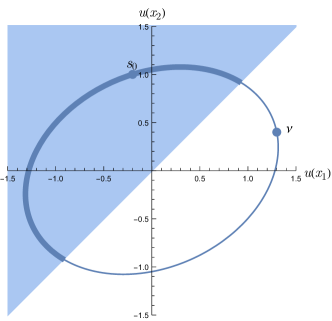
Figure 2: Sampling from a constrained region using lin-ess,

The only parameters in the model are the hyperparameters $\bm{\theta}$ in the kernel function. Since the utility function is invariant under increasing transformations, the scale (variance) parameter $\sigma_{k}^{2}$ in (1) is not identifiable. Therefore, we assume that $\sigma_{k}^{2}=1$. The other hyperparameters can be selected by maximising the marginal likelihood:

$$\hat{\bm{\theta}}=\arg\max_{\bm{\theta}\in\Theta}p(\mathcal{D}_{m}|\bm{\theta})~{}\text{ with }~{}p(\mathcal{D}_{m}|\bm{\theta})=\int I_{\{Wu(X)\geq 0\}}(u(X))N(u(X);\mathbf{0},K_{\bm{\theta}}(X,X))du(X).$$ (10)

The integral in (10) is intractable. There are a variety of approximate inference techniques that one can resort to. We use the following approach: (a) we approximate the indicator function with a sigmoid-type function; (b) we perform a local expansion of the integrand around its maximum and then analytically compute the integral. Note that, the step (b) corresponds to the Laplace’s approximation (Rasmussen and Williams, 2006).

Example 4

Our aim is to infer Alice’s utility $u({\bf x})$ from the dataset of pairwise preferences $\mathcal{D}_{19}$ in Example 1. We will then use the learned model to predict Alice’s preference for $20\stackrel{{\scriptstyle?}}{{\succ}}18$. As described in this section, we place a GP prior on $u$ and use the SE kernel in (1) with $\sigma_{k}^{2}=1$. The value of the lengthscale is fixed to $\hat{\ell}=1.5$. We then sample 60,000 samples of $u(X)$ from the posterior with lin-ess, and compute the predictive posterior for $200$ equally spaced temperatures in the interval $[10,25]$. Figure 3(a)-left shows the corresponding mean and 95% credible interval. The uncertainty is high due to the small dataset.

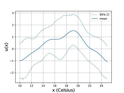
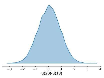
(a) 20 pairwise preferences

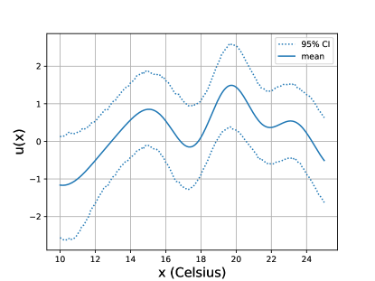
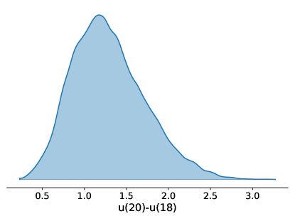
(b) 40 pairwise preferences

Figure 3: Left: learned utility functions, the mean is the continuous line and the region between the dotted-lines is the 95% credible region. Right: posterior marginal of the difference $u(20)-u(18)$.

This is the advantage of using a Bayesian approach to estimate the utility function $u$: it quantifies the uncertainty of its own estimate. Indeed, the trained model is undecided about $u(20)-u(18)\stackrel{{\scriptstyle?}}{{>}}0$ as shown by the distribution in Figure 3(a)-right (the pair $18,20$ is not included in the dataset). Note in fact that, the predictive posterior for $u(20)-u(18)$ has mass over both the positive and negative values. The uncertainty decreases if we consider 40 pairwise preferences as shown in Figure 3(b)-left (compare it with Figure 1). From Figure 3(b)-right, we conclude that $u(20)-u(18)>0$ with probability $\approx 1$, that is Alice prefers the temperature $20$ to $18$. Note that, also in this case, the pair $18,20$ is not included in the dataset.

The model is summarised in the following box.

Model 1: Consistent Preferences
Consider a vector $X=[{\bf x}_{1},{\bf x}_{2},\dots,{\bf x}_{r}]^{\top}$ of objects such that ${\bf x}_{i}\in\mathbb{R}^{c}$ for all $i=1,\dots,r$ and a training set of $m$ preferences $\mathcal{D}_{m}=\{{\bf x}_{i_{s}}\succ{\bf x}_{j_{s}}:~{}~{}s=1,\dots,m\}$ with ${\bf x}_{i_{s}}\neq{\bf x}_{j_{s}}$, ${\bf x}_{i_{s}},{\bf x}_{j_{s}}\in X$, $i_{s},j_{s}\in\{1,2,\dots,r\}$ for each $s=1,\dots,m$. Assuming the preferences are consistent, there exists a utility function $u$ which represents them. Then, the probability of observing the data $\mathcal{D}_{m}$ given the utility function vector $u(X)$ is equal to the likelihood function:

$$p(\mathcal{D}_{m}|u(X))=\prod_{s=1}^{m}I_{\{u({\bf x}_{i_{s}})-u({\bf x}_{j_{s}})>0\}}(u(X))=I_{\{Wu(X)>0\}}(u(X)).$$ (11)

Assuming a GP prior $p(u)=\mathrm{GP}(u;0,k_{\bm{\theta}})$, the predictive posterior for $u(X^{*})$ given the test-points $X^{*}=[{\bf x}_{1},\dots,{\bf x}_{p}]$ is

$$p(u(X^{*})|\mathcal{D}_{m})=\int p(u(X^{*})|u(X))\;TN_{\{Wu(X)\geq 0\}}(u(X);\mathbf{0},K_{\bm{\theta}}(X,X))du(X),$$ (12)

where $p(u(X^{*})|u(X))$ is defined in (9).

3.2 Problems arising in the modelling of preference relations

What if the preferences of a subject are irrational? Alice’s preferences may fail to satisfy asymmetry and/or negative transitivity for a number of reasons.

1. Limit of discernibility. As discussed in Section 2.1, all asymmetric and negatively transitive preference relations can be thought to be originated by a utility function according to:

   $${\bf x}\succ{\bf y}~{}\textit{ iff }~{}u({\bf x})>u({\bf y}).$$

   However, consider two objects ${\bf x},{\bf y}$ whose utilities can barely be discerned by Alice, and a third object ${\bf z}$ whose utility is between that of ${\bf x}$ and ${\bf y}$. In this case, Alice may either not be able to state her preference for ${\bf z}$ compared to ${\bf x},{\bf y}$ (violating negative transitivity), or state a wrong preference (violating asymmetry or negative transitivity).

2. Additive noise. Another potential issue arises in the case the observed utility function differs from the true utility function (due to disturbances, measurement errors). In this situation, Alice states ${\bf x}\succ{\bf y}$ if the observed utility of ${\bf x}$ is greater than the observed utility of ${\bf y}$, i.e., $o({\bf x})>o({\bf y})$. The observation error is commonly assumed to be additive Gaussian, that is $o({\bf x})=u({\bf x})+v_{x}$ and $o({\bf y})=u({\bf y})+v_{y}$, where $v_{x},v_{y}$ are two independent and Gaussian distributed variables with zero mean and variance $\sigma^{2}_{v}$. Due to the observation error, preferences may violate asymmetry or negative transitivity or both.

3. Multiple utilities. Often the apparently violation of asymmetry and negative transitivity can be explained as the result of the intersection of several primitive preferences. For instance in the home-temperature example Alice may compare temperatures based on two utility functions: relax $u_{1}$ and fitness $u_{2}$. Given two temperatures ${\bf x},{\bf y}$, Alice may prefer ${\bf x}\succ{\bf y}$ under $u_{1}$ and ${\bf y}\succ{\bf x}$ under $u_{2}$ leading to conflictual preferences.

We will now discuss how we can change the previous model to account for these issues.

3.2.1 Accounting for the limit of discernibility

In order to account for the limit of discernibility, we can employ a cardinal utility function, that is the difference $u({\bf x})-u({\bf y})$ is used as a measure of the similarity between ${\bf x},{\bf y}$. We will consider two models.

Luce’s model:

Following a model introduced by Luce (1956), the relation $\succ$ is represented by a pair $(u,\delta)$ where $u$ is a utility function and $\delta>0$ is a threshold – called the just noticeable difference – such that

$${\bf x}\succ{\bf y}~{}~{}\textit{ iff }~{}~{}u({\bf x})>u({\bf y})+\delta.$$ (13)

In other words, Alice states ${\bf x}\succ{\bf y}$ only if the difference between the utility functions of the two items is larger than the threshold $\delta$ (which is the limit of discernibility). The relation defined in (13) satisfies asymmetry and transitivity (but not negative transitivity).

In the absence of strict preference between two alternatives ${\bf x},{\bf y}$, that is, if neither ${\bf x}\succ{\bf y}$ nor ${\bf y}\succ{\bf x}$ holds, then Alice will state that there is no noticeable difference between the two objects, denoted as ${\bf x}\smile{\bf y}$, that is

$${\bf x}\smile{\bf y}~{}~{}\textit{ iff }~{}~{}|u({\bf x})-u({\bf y})|\leq\delta.$$ (14)

The relation $\smile$ is not an indifference relation because it is reflexive, symmetric but it is not transitive. We can easily modify the consistent preferences learning model presented in Section 3.1 to account for the limit of discernibility under Luce’s model.

Model 2: Just Noticeable Difference
Consider a vector $X=[{\bf x}_{1},{\bf x}_{2},\dots,{\bf x}_{r}]^{\top}$ of objects such that ${\bf x}_{i}\in\mathbb{R}^{c}$ for all $i=1,\dots,r$, a training set of $m_{a}$ preferences denoted as $\mathcal{D}_{m_{a}}=\{{\bf x}_{i_{s}}\succ{\bf x}_{j_{s}}:~{}~{}s=1,\dots,m_{a}\}$ and $m_{b}$ indiscernibility statements denoted as $\mathcal{D}_{m_{b}}=\{{\bf x}_{i_{s}}\smile{\bf x}_{j_{s}}:~{}~{}s=1,\dots,m_{b}\}$ with ${\bf x}_{i_{s}}\neq{\bf x}_{j_{s}}$, ${\bf x}_{i_{s}},{\bf x}_{j_{s}}\in X$, $i_{s},j_{s}\in\{1,2,\dots,r\}$ for each $s$. Under (13), we can rewrite these sets as $\mathcal{D}_{m_{a}}=\{\frac{1}{\delta}(u({\bf x}_{i_{s}})-u({\bf x}_{j_{s}}))>1:~{}~{}s=1,\dots,m_{a}\}$ and $\mathcal{D}_{m_{b}}=\{\frac{1}{\delta}|u({\bf x}_{i_{s}})-u({\bf x}_{j_{s}})|\leq 1:~{}~{}s=1,\dots,m_{b}\}$. Then, the probability of observing the data $\mathcal{D}_{m_{a}},\mathcal{D}_{m_{b}}$ given the utility function vector $u(X)$ is equal to the likelihood function:

$$p(\mathcal{D}_{m_{a}},\mathcal{D}_{m_{b}}|u(X))=p(\mathcal{D}_{m_{a}}|u(X))p(\mathcal{D}_{m_{b}}|u(X)),$$ (15)

$$p(\mathcal{D}_{m_{a}}|u(X))=\prod_{s=1}^{m_{a}}I_{\left\{\frac{1}{\delta}(u({\bf x}_{i_{s}})-u({\bf x}_{j_{s}}))>1\right\}}=I_{\left\{-W_{a}\frac{u(X)}{\delta}<-\mathbf{1}_{m_{a}}\right\}}(u(X)),$$ (16)

$$p(\mathcal{D}_{m_{b}}|u(X))=\prod_{s=1}^{m_{b}}I_{\left\{\frac{1}{\delta}\left(u({\bf x}_{i_{s}})-u({\bf x}_{j_{s}})\right)\leq 1\right\}}I_{\left\{\frac{1}{\delta}\left(u({\bf x}_{j_{s}})-u({\bf x}_{i_{s}})\right)\leq 1\right\}}=I_{\left\{W_{b}\frac{u(X)}{\delta}\leq\mathbf{1}_{2m_{b}}\right\}}(u(X)),$$ (17)

where $\mathbf{1}_{d}$ is the unit-vector of dimension $d$, $W_{a}\in\mathbb{R}^{m_{a}\times r},~{}W_{b}\in\mathbb{R}^{2m_{b}\times r}$ are matrices representing the linear constraints. By defining $W=[-W_{a}^{\top},W_{b}^{\top}]^{\top}$, $\mathbf{c}=[-\mathbf{1}_{m_{a}}^{\top},\mathbf{1}_{2m_{b}}^{\top}]^{\top}$, $u^{\prime}(\cdot)=\frac{u(\cdot)}{\delta}$ and assuming a GP prior $p(u^{\prime})=\mathrm{GP}(u^{\prime};0,k_{\bm{\theta}})$, the predictive posterior for $u^{\prime}(X^{*})$ given the test-points $X^{*}=[{\bf x}_{1},\dots,{\bf x}_{p}]$ is

$$p(u^{\prime}(X^{*})|\mathcal{D}_{m_{a}},\mathcal{D}_{m_{b}})=\int p(u^{\prime}(X^{*})|u^{\prime}(X))\;TN_{\{Wu^{\prime}(X)\leq\mathbf{c}\}}(u^{\prime}(X);\mathbf{0},K_{\bm{\theta}}(X,X))du^{\prime}(X),$$ (18)

with $p(u^{\prime}(X^{*})|u^{\prime}(X))$ as in (9).

After rescaling $u^{\prime}(\cdot)=\frac{u(\cdot)}{\delta}$, the only parameters in the model are the hyperparameters $\bm{\theta}$ in the kernel function. The scale (variance) parameter $\sigma_{k}^{2}$ in (1) is weakly identifiable in this case, because the inequality $|u^{\prime}({\bf x}_{i})-u^{\prime}({\bf x}_{j})|\leq 1$ determines the level of discernibility. The hyperparameters $\bm{\theta}$ can be selected by maximising the marginal likelihood using the same approach described in Section 3.1. The computation of posterior and predictive posterior inferences can again be performed via sampling using lin-ess.

Example 5

We consider the home-temperature example, whose true utility function is shown in Figure 1. We assume that two temperatures ${\bf x}_{i},{\bf x}_{j}$ are indiscernible by Alice whenever $|u({\bf x}_{i})-u({\bf x}_{j})|\leq 0.025$ In order to infer Alice’s utility function, we consider the set of temperatures (objects) $\mathcal{X}=\{10,11,12,\dots,25\}$ and asks her preferences for $19$ pairs of temperatures. This results in the datasets:

$$\mathcal{D}_{17}= \{12\succ 10,13\succ 25,14\succ 13,15\succ 22,15\succ 23,16\succ 11,19\succ 22,19\succ 24,20\succ 10,$$

$$20\succ 14,20\succ 21,20\succ 24,20\succ 25,21\succ 13,21\succ 25,23\succ 25,24\succ 25\},$$ (19)

$$\mathcal{D}_{2}= \{15\smile 19,19\smile 21\},$$ (20)

where $\mathcal{D}_{2}$ includes two indiscernible pairs of temperatures. We aim to learn Alice’s utility $u^{\prime}$ from the above datasets and predict her preferences for any other pairs of temperatures.

We place a GP prior on $u^{\prime}$ with a SE kernel. Figure 4(a)-left shows the predictive posterior mean and 95% credible interval for $u^{\prime}$. The uncertainty is high due to the small dataset. Indeed, note that the model is undecided about $|u(13)-u(18)|\stackrel{{\scriptstyle?}}{{\leq}}1$ as shown by the distribution in Figure 4(a). Instead, we can conclude with certainty that $15,19$ are indiscernible and $20\succ 18$ with high probability. The uncertainty decreases if we consider 40 pairwise preferences as shown in Figure 4(b). From Figure 4(b), we conclude that $u(20)-u(18)>0$ with probability $\approx 1$, that is Alice prefers the temperature $20$ to $18$. There is also high probability that the temperatures $13$ to $18$ are indiscernible for Alice.

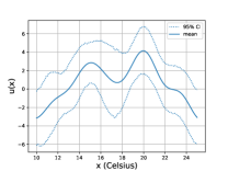
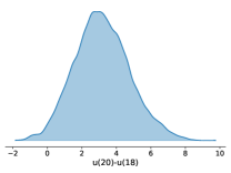
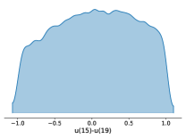
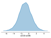
(a) 20 pairwise preferences

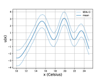
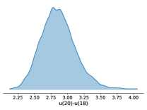
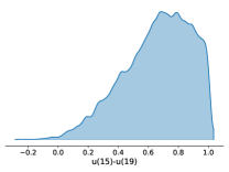
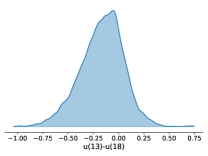
(b) 40 pairwise preferences

Figure 4: Left: learned utility functions under Luce’s model, the mean is the continuous line and the region between the dotted-lines is the 95% credible region. The other three figures are the posterior marginals of $u(20)-u(18)$, $u(15)-u(19)$ and, respectively, $u(13)-u(18)$.

Erroneous preferences model

Luce introduced an interval of no noticeable difference to model Alice’s absence of strict preference between two indiscernible objects ${\bf x},{\bf y}$. However, there are applications where Alice is forced to express her preference between ${\bf x},{\bf y}$ even when the two objects are indiscernible.

This will result in wrong preference statements – Alice may state ${\bf y}\succ{\bf x}$ when $u({\bf x})>u({\bf y})$ – overall leading to violations of asymmetry and negative transitivity. The probability of correctly stating ${\bf x}\succ{\bf y}$ is a function of the difference $u({\bf x})-u({\bf y})$, which can be modelled by the following likelihood:

$$p({\bf x}\succ{\bf y}|u)=\Phi\left(\frac{u({\bf x})-u({\bf y})}{\sigma}\right),$$ (21)

where $\Phi(\cdot)$ is the Cumulative Distribution Function (CDF) of the standard Normal distribution. $\sigma>0$ is a scaling parameter, which plays a similar role to $\delta$ in Luce’s model. As shown in Figure 5, for a given value of $\Delta_{u}=u({\bf x})-u({\bf y})$, the probability of stating the correct preference decreases with $\sigma$.

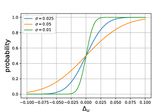
Figure 5: $\Phi(\Delta_{u}/\sigma)$ for different values of $\sigma$.

In statistics, the likelihood (21) is known as probit.

Hereafter we exploit a result derived in (Benavoli et al., 2021a) to show that, assuming a GP prior on $u$ and the likelihood (21), the predictive posterior for $u$ is a Skew-GP.

Model 3: Probit model for erroneous preferences
Consider a vector $X=[{\bf x}_{1},{\bf x}_{2},\dots,{\bf x}_{r}]^{\top}$ of objects such that ${\bf x}_{i}\in\mathbb{R}^{c}$ for all $i=1,\dots,r$, a training set of $m$ preferences $\mathcal{D}_{m}=\{{\bf x}_{i_{s}}\succ{\bf x}_{j_{s}}:~{}~{}s=1,\dots,m\}$ with ${\bf x}_{i_{s}}\neq{\bf x}_{j_{s}}$, ${\bf x}_{i_{s}},{\bf x}_{j_{s}}\in X$, for all $i_{s},j_{s}\in\{1,2,\dots,r\}$. Under the assumption that the preference statements are conditionally independent give $u(X)$ and introducing $u^{\prime}(\cdot)=u(\cdot)/\sigma$, from (21) we obtain that:

$$p(\mathcal{D}_{m}|u^{\prime}(X))=\prod_{s=1}^{m}\Phi\left(u^{\prime}({\bf x}_{i_{s}})-u^{\prime}({\bf x}_{j_{s}})\right)=\Phi_{m}(Wu^{\prime}(X)),$$ (22)

where $W$ has been defined in Section 3.1 and $\Phi_{m}(\cdot)$ is the CDF of the standard $m$-dimensional multivariate normal distribution.

Assuming $p(u^{\prime})=\mathrm{GP}(u^{\prime};0,k_{\bm{\theta}})$, the predictive posterior $u^{\prime}(X^{*})$ for the test-points $X^{*}=[{\bf x}_{1},\dots,{\bf x}_{p}]$ is a Skew GP of dimension $m$:

$$p(u^{\prime}(X^{*})|\mathcal{D}_{m})=\text{SkewGP}_{m}( {\bf 0},K_{\bm{\theta}}(X^{*},X^{*}),D_{K_{\bm{\theta}}(X^{*},X^{*})}^{-1}K_{\bm{\theta}}(X^{*},X)W^{T},$$

$${\bf 0},WK_{\bm{\theta}}(X,X)W^{T}+I_{m}),$$ (23)

where $D_{K_{\bm{\theta}}(X^{*},X^{*})}$ is a diagonal matrix equal to the square-root of the diagonal of $K_{\bm{\theta}}(X^{*},X^{*})$. The distribution (23) has 5 parameters, the first (zero) is a location parameter, the second $K_{\bm{\theta}}(X^{*},X^{*})$ is the Kernel matrix, the last three parameters determine the skewness of the distribution. More details about the Skew Gaussian distribution and the Skew GP are provided in Appendix B.

It is worth pointing out that, even when Alice’s preferences in $\mathcal{D}_{m}$ do not satisfy asymmetry and negative transitivity, the posterior is always well-defined in this case, because the model explicitly takes into account of the inconsistencies (errors) in Alice’s preferences.

At first, the predictive posterior in (23) might appear to be quite complex. However, the computation of predictive inferences (mean, credible intervals etc.) can easily be achieved by sampling from the predictive posterior (Benavoli et al., 2021a, Sec. 4):

$$u(X^{*}) =\mathbf{r}_{0}+K_{\bm{\theta}}(X^{*},X)W^{T}\left(WK_{\bm{\theta}}(X,X)W^{T}+I_{m}\right)^{-1}\mathbf{r}_{1},$$

$$\mathbf{r}_{0} \sim N\left({\bf 0},K_{\bm{\theta}}(X^{*},X^{*})-K_{\bm{\theta}}(X^{*},X)W^{T}\left(WK_{\bm{\theta}}(X,X)W^{T}+I_{m}\right)^{-1}WK_{\bm{\theta}}(X,X^{*})\right),$$

$$\mathbf{r}_{1} \sim\text{TN}_{\{u^{\prime}(X)\geq{\bf 0}\}}\left({\bf 0},WK_{\bm{\theta}}(X,X)W^{T}+I_{m}\right).$$

We sample $\mathbf{r}_{1}$ using lin-ess.

After rescaling $u^{\prime}(\cdot)=\frac{u(\cdot)}{\sigma}$, the only parameters in the model are the hyperparameters $\bm{\theta}$ in the kernel function. The scale (variance) parameter $\sigma_{k}^{2}$ is identifiable in this case, because the probability of correctly stating a preference ${\bf x}_{i}\succ{\bf x}_{j}$ is a function of the difference $u^{\prime}({\bf x}_{i})-u^{\prime}({\bf x}_{j})$. The hyperparameters $\bm{\theta}$ can be selected by maximising the marginal likelihood. The computation of the marginal likelihood requires the calculation of the CDF of the $m$-dimensional multivariate normal distribution. To approximate this integral, we can use the same approach described in Section 3.1. However, since the likelihood is already a soft indicator, we do not need to approximate it in this case.

Example 6

As before, we consider the set of temperatures $\mathcal{X}=\{10,11,12,\dots,25\}$ and asks Alice preferences for $19$ pairs of temperatures. We generate Alice’s preferences according to the model in (21) with $u$ as in Figure 1 and $\sigma=0.05$. This results in the dataset:

$$\mathcal{D}_{19}= \{12\succ 10,13\succ 25,14\succ 13,15\succ 19,15\succ 22,15\succ 23,16\succ 11,19\succ 22,19\succ 24,20\succ 10,$$

$$20\succ 14,20\succ 21,20\succ 24,20\succ 25,21\succ 13,21\succ 19,21\succ 25,23\succ 25,24\succ 25\}.$$ (24)

By comparing (4) and (24), it can be noted the following errors in Alice’s preferences $15\succ 19$ and $21\succ 19$. In order to learn Alice’s utility $u^{\prime}$ from $\mathcal{D}_{19}$, we place a GP prior on $u^{\prime}$ with a SE kernel and compute the predictive posterior as described in this section.

Figure 6(a)-left shows the predictive posterior mean and 95% credible interval for $u^{\prime}$. The model is undecided about $u(20)-u(18)\stackrel{{\scriptstyle?}}{{\geq}}0$. The uncertainty decreases if we consider 40 pairwise preferences as shown in Figure 6(b): correctly the model states that $u(20)-u(18)\geq 0$ with probability $\approx 1$, that is we can infer that Alice prefers the temperature $20$ to $18$.

Figures 7(a) show that the model performs well also when preferences are generated using $\sigma=0.2$, which leads to datasets $\mathcal{D}_{m}$ including many more errors.

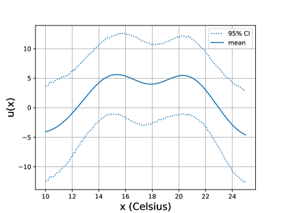
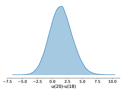
(a) 20 pairwise preferences

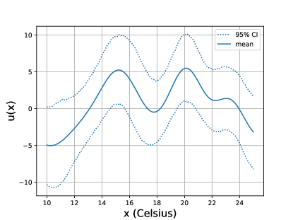
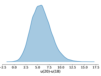
(b) 40 pairwise preferences

Figure 6: Left: learned utility functions under the probit model for erroneous preference, the mean is the continuous line and the region between the dotted-lines is the 95% credible region. Right: posterior marginal of the difference $u(20)-u(18)$. The preferences were generated using $\sigma=0.05$.

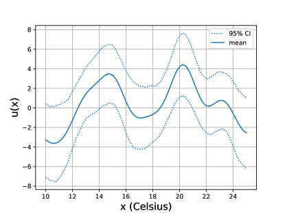
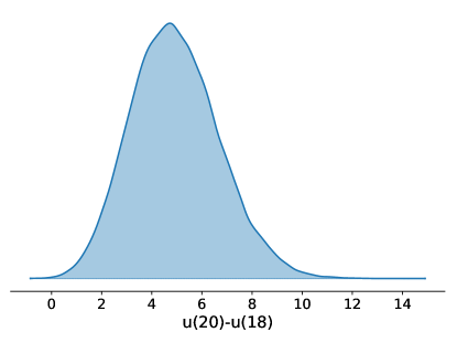
(a) 40 pairwise preferences

Figure 7: Left: learned utility functions under the probit model for erroneous preference, the mean is the continuous line and the region between the dotted-lines is the 95% credible region. Right: posterior marginal of the difference $u(20)-u(18)$. The preferences were generated using $\sigma=0.2$.

By comparing (5) and (22), it can be noticed that the indicator function in (5) has been replaced in (22) by a sigmoid function (soft indicator).

3.2.2 Convergence of the Probit model to the consistent preferences model

In the case of erroneous preferences, the probit model introduced above has a special relationship with the consistent preferences model. The parameter $\sigma$ in (21) determines how “erroneous” the observed preferences are. For small values of $\sigma$ the probit and the consistent preferences model become very similar. This relationship can be formalised as follows

Proposition 10

Consider a vector $X=[{\bf x}_{1},{\bf x}_{2},\dots,{\bf x}_{r}]^{\top}$ of objects such that ${\bf x}_{i}\in\mathbb{R}^{c}$ for all $i=1,\dots,r$, a training set of $m$ preferences $\mathcal{D}_{m}=\{{\bf x}_{i_{s}}\succ{\bf x}_{j_{s}}:~{}~{}s=1,\dots,m\}$ with ${\bf x}_{i_{s}}\neq{\bf x}_{j_{s}}$, ${\bf x}_{i_{s}},{\bf x}_{j_{s}}\in X$, $i_{s},j_{s}\in\{1,2,\dots,r\}$ for each $s=1,\dots,m$ and the likelihood of the probit model given by:

$$p(\mathcal{D}_{m}|u(X))=\prod_{s=1}^{m}\Phi\left(\dfrac{u({\bf x}_{i_{s}})-u({\bf x}_{j_{s}})}{\sigma}\right)=\Phi_{m}\left(W\dfrac{u(X)}{\sigma}\right),$$ (25)

where we kept the non-scaled GP process $u$. Assuming the preferences are consistent, then the likelihood in (25) converges to the likelihood in (11) as $\sigma\rightarrow 0$.

Proof  For any $s\in\{1,\ldots,m\}$ we have

$$\lim_{\sigma\rightarrow 0}\Phi\left(\dfrac{u({\bf x}_{i_{s}})-u({\bf x}_{j_{s}})}{\sigma}\right)=\begin{cases}0&\text{if }u({\bf x}_{i_{s}})-u({\bf x}_{j_{s}})<0\\ 1&\text{if }u({\bf x}_{i_{s}})-u({\bf x}_{j_{s}})>0\end{cases}=I_{\{u({\bf x}_{i_{s}})-u({\bf x}_{j_{s}})>0\}}(u(X)),$$

by the properties of the Gaussian CDF $\Phi$. Note that $p(\mathcal{D}_{m}|u(X))=\prod_{s=1}^{m}\Phi\left(\dfrac{u({\bf x}_{i_{s}})-u({\bf x}_{j_{s}})}{\sigma}\right)$, thus we obtain the result.  

For this reason, it is common in practice to employ the probit-likelihood model even when the subject’s preferences are known to be consistent.

3.2.3 The Gaussian noise model

In many situations, the observed utility $o({\bf x}),o({\bf y})$ of two objects ${\bf x},{\bf y}$ may differ from the true utility $u({\bf x}),u({\bf y})$ due to noise in the observation process. This observation noise is commonly modelled by using an additive Gaussian model (Thurstone, 1927; Chu and Ghahramani, 2005), that is $o({\bf x})=u({\bf x})+v_{x}$ and $o({\bf y})=u({\bf y})+v_{y}$, where $v_{x},v_{y}$ are two independent and Gaussian distributed variables with zero mean and variance $\sigma^{2}$. Due to this noise, preferences can therefore violate asymmetry or negative transitivity or both.

It is interesting to note that, for a preference statement, ${\bf x}\succ{\bf y}$, the likelihood:

$$p({\bf x}\succ{\bf y}|u(X)) =\int I_{\{u({\bf x})+v_{x}>u({\bf y})+v_{y}\}}(v_{x},v_{y})N\left(v_{x};0,\sigma^{2}\right)N\left(v_{y};0,\sigma^{2}\right)dv_{x}dv_{y}=\Phi\left(\frac{u({\bf x})-u({\bf y})}{\sqrt{2}\sigma}\right),$$ (26)

reduces to the likelihood model in (21). The only distinction is the constant $\sqrt{2}$. However, the main difference between the erroneous-preference model and the Gaussian noise model becomes evident when we compare more than two objects. Consider for instance the preferences ${\bf x}\succ{\bf y}$ and ${\bf x}\succ{\bf z}$, the likelihood

$$p({\bf x}\succ{\bf y},{\bf x}\succ{\bf z}|u(X)) =\int I_{\left\{\begin{subarray}{c}u({\bf x})+v_{x}>u({\bf y})+v_{y},\\ u({\bf x})+v_{x}>u({\bf z})+v_{z}\end{subarray}\right\}}(v_{x},v_{y},v_{z})N\left(v_{x};0,\sigma^{2}\right)N\left(v_{y};0,\sigma^{2}\right)N\left(v_{z};0,\sigma^{2}\right)dv_{x}dv_{y}dv_{z}$$ (27)

$$\neq\Phi\left(\frac{u({\bf x})-u({\bf y})}{\sqrt{2}\sigma}\right)\Phi\left(\frac{u({\bf x})-u({\bf z})}{\sqrt{2}\sigma}\right),$$

due to the common noise $v_{x}$ in the two preference statements. There is a straightforward way to account for the common noise in the preference. We can simply use an augmented prior

$$\begin{bmatrix}u(X)\\ v(X)\end{bmatrix}\sim N\left(\begin{bmatrix}{\bf 0}_{m}\\ {\bf 0}_{m}\end{bmatrix},\begin{bmatrix}K_{\bm{\theta}}(X,X)&{\bf 0}_{m\times m}\\ {\bf 0}_{m\times m}&\sigma^{2}I_{m}\end{bmatrix}\right)$$ (28)

with $v(X)=[v_{x_{1}},\dots,v_{x_{m}}]^{\top}$ and consider the indicator likelihood.

Model 4: Preferences with Gaussian noise error
Consider a vector $X=[{\bf x}_{1},{\bf x}_{2},\dots,{\bf x}_{r}]^{\top}$ of objects such that ${\bf x}_{i}\in\mathbb{R}^{c}$ for all $i=1,\dots,r$ and a training set of $m$ preferences $\mathcal{D}_{m}=\{{\bf x}_{i_{s}}\succ{\bf x}_{j_{s}}:~{}~{}s=1,\dots,m\}$ with ${\bf x}_{i_{s}}\neq{\bf x}_{j_{s}}$, ${\bf x}_{i_{s}},{\bf x}_{j_{s}}\in X$, $i_{s},j_{s}\in\{1,2,\dots,r\}$ for each $s=1,\dots,m$. Assuming the preferences are noisy due to an additive Gaussian noise. Then, the probability of observing the data $\mathcal{D}_{m}$ given the utility function vector $u(X)$ and the noise vector $v(X)$ is equal to the likelihood function:

$$p(\mathcal{D}_{m}|u(X),v(X)) =\prod_{s=1}^{m}I_{\{u({\bf x}_{i_{s}})+v_{i_{s}}-u({\bf x}_{j_{s}})-v_{j_{s}}>0\}}(u(X),v(X))$$ (29)

$$=I_{\left\{\widetilde{W}\begin{bmatrix}u(X)\\ v(X)\end{bmatrix}>0\right\}}(u(X),v(X)),$$

where $\widetilde{W}$ is a suitable matrix which allows to rewrite the inequalities in the indicator in matrix-form. Assuming a GP prior $p(u)=\mathrm{GP}(u;0,k_{\bm{\theta}})$, the predictive posterior for $u(X^{*})$ given the test-points $X^{*}=[{\bf x}_{1},\dots,{\bf x}_{p}]$ is

$$p(u(X^{*})|\mathcal{D}_{m})=\int p(u(X^{*})|u(X))$$ (30)

$$TN_{\left\{\widetilde{W}\begin{bmatrix}u(X)\\ v(X)\end{bmatrix}>0\right\}}\left(\begin{bmatrix}u(X)\\ v(X)\end{bmatrix};\begin{bmatrix}{\bf 0}_{m}\\ {\bf 0}_{m}\end{bmatrix},\begin{bmatrix}K_{\bm{\theta}}(X,X)&{\bf 0}_{m\times m}\\ {\bf 0}_{m\times m}&\sigma^{2}I_{m}\end{bmatrix}\right)du(X)dv(X)$$

where $p(u(X^{*})|u(X))$ is defined in (9).

Note that, the above model is structurally similar to Model 3.1. Therefore, we can use the same approach to compute the predictive distribution (30) via lin-ess and to learn the hyperparameters $\bm{\theta},\sigma^{2}$.

Finally, observe that, if the pairs in the preference dataset are unique (the same object is only compared once), this model is equivalent to Model 3.2.1.

Example 7

We consider the set of temperatures $\mathcal{X}=\{10,11,12,\dots,25\}$ and, for each temperature, we generated a realisation of observed temperature $o(x_{i})=u(x_{i})+v(x_{i})$, with $u$ as in Figure 1 and $v(x_{i})$ sampled from independent Gaussian distributions with $\sigma=0.1$. We then generated $80$ random pairwise preferences (without repetitions) as follows: $x_{i}\succ x_{j}$ if $o(x_{i})>o(x_{j})$. This could represent a situation where drafts in the house perturb Alice’s utility.

We compared two models. Figure 8-left displays the posterior utility (mean and credible interval) obtained from Model 3.2.3, which accounts for the common noise in the preference statements. Figure 8-right shows the posterior utility derived from Model 3.2.1, which ignores the common noise. We can see that Model 3.2.1 wrongly fits the noise and produces an incorrect estimate of the function. Moreover, the uncertainty is clearly underestimated. This demonstrates that modelling the common noise correctly is very important in practice.

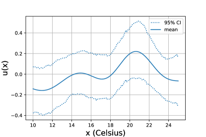
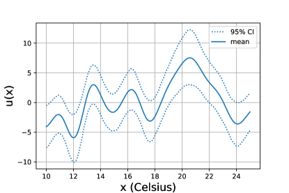
Figure 8: Left: learned utility functions under the Gaussian-noise model for preferences, the mean is the continuous line and the region between the dotted-lines is the 95% credible region. Right: learned utility functions under the Probit model for preferences.

3.2.4 Multiple implicit utility functions

In some applications, there may be a variety of attributes to consider while comparing objects. Therefore, Alice’s preference ${\bf x}\succ{\bf y}$ may be determined by multiple utility functions $u_{1},\dots,u_{d}$ taking into account different characteristics of the objects under consideration:

$$u_{1}({\bf x}),\dots,u_{d}({\bf x})~{}\text{ versus }~{}u_{1}({\bf y}),\dots,u_{d}({\bf y}).$$

We assume that both the functions $u_{i}$ and the dimension $d$ are unknown and consider two cases.

1. When expressing her judgements, Alice is able to aggregate the multiple utility functions into a single dimension. For instance, she can implicitly consider the additive aggregation:

   $$u({\bf x})=u_{1}({\bf x})+\dots+u_{d}({\bf x}).$$

   By assuming that the aggregated function $u$ is the unknown utility, we are back to the single utility model.

2. Alice judges an object to be better than another object if for instance it is better with respect to all attributes (Pareto efficiency), leading to the relations:

   $${\bf x}\succ{\bf y}\text{ iff } \min_{i}(u_{i}({\bf x})-u_{i}({\bf y}))>0,$$ (31)

   $${\bf x}\frown{\bf y}\text{ iff } \max_{i}(u_{i}({\bf x})-u_{i}({\bf y}))>0~{}\&~{}\min_{i}(u_{i}({\bf x})-u_{i}({\bf y}))<0,$$ (32)

   where ${\bf x}\frown{\bf y}$ means that there is a conflict, that is neither ${\bf x}$ nor ${\bf y}$ is judged to be better with respect to all attributes.

The relation $\succ$ in (31) is asymmetric but is not negatively transitive. The relation $\frown$ is not an indifference relation, because is not transitive.

We can extend Model 3.2.1 to handle multiple utilities. Specifically, we replace the strict statements (31)–(32) with the probit likelihood to account for errors due to Alice’s inability to distinguish two objects that have similar utility $u_{i}$ for $i=1,\dots,d$. This leads to the following likelihood:

$$p({\bf x}\succ{\bf y}|u_{1},\dots,u_{d}) =\prod_{i=1}^{d}\Phi\left(\frac{u_{i}({\bf x})-u_{i}({\bf y})}{\sigma}\right),$$ (33)

$$p({\bf x}\frown{\bf y}|u_{1},\dots,u_{d}) =1-\prod_{i=1}^{d}\Phi\left(\frac{u_{i}({\bf x})-u_{i}({\bf y})}{\sigma}\right)-\prod_{i=1}^{d}\Phi\left(\frac{u_{i}({\bf y})-u_{i}({\bf x})}{\sigma}\right).$$ (34)

Note that, (33) and (34) are probabilistic relaxations of (31) and, respectively, (32).

We will defer the discussions on multiple utilities for preferences over objects until Section 5, where we will introduce a more general model based on choice functions.

3.3 Representation via two-argument functions

A binary relation $R$ on $\mathcal{X}\times\mathcal{X}$ can be represented through a two-argument function $q:\mathcal{X}\times\mathcal{X}\rightarrow\mathbb{R}$. If $({\bf x},{\bf y})\in R$, denoted as ${\bf x}R{\bf y}$, then $q({\bf x},{\bf y})>0$. Since in general $q({\bf x},{\bf y})\neq q({\bf y},{\bf x})$ we can equivalently write $q({\bf x},{\bf y})$ as $q([{\bf x},{\bf y}])$, that is as a function of the vector $[{\bf x},{\bf y}]$. The function $q$ has been interpreted as a “strength of preference” (Shafer, 1974; Fishburn, 1988), with values of $q([{\bf x},{\bf y}])$ close to zero indicating a difficult decision (the decision maker cannot distinguish ${\bf x},{\bf y}$).

This is a natural generalisation of representation results for consistent preferences, in which case one can set $q([{\bf x},{\bf y}])=u({\bf x})-u({\bf y})$ for a utility function $u$. In this case, from the asymmetry property of preferences, we can derive that $q$ must be a skew-symmetric function $q([{\bf x},{\bf y}])=-q([{\bf y},{\bf x}])$. Moreover, $q$ must satisfy negative transitivity – if $q([{\bf x},{\bf y}])>0$ then for any other ${\bf z}\in\mathcal{X}$ either $q([{\bf x},{\bf z}])>0$ or $q([{\bf z},{\bf y}])>0$ or both. This follows by $q([{\bf x},{\bf y}])=u({\bf x})-u({\bf y})=(u({\bf x})-u({\bf z}))-(u({\bf y})-u({\bf z}))$.

In the case $q([{\bf x},{\bf y}])=u({\bf x})-u({\bf y})$, we can observe that a GP prior on $u$ induces a GP prior on $q$, because Gaussianity is preserved by affine transformations. It is easy to show that if $u\sim GP(0,k_{\bm{\theta}}({\bf x},{\bf x}^{\prime}))$, then $q\sim GP(0,k_{pref}([{\bf x},{\bf y}],[{\bf x}^{\prime},{\bf y}^{\prime}]))$ where

$$k_{pref}([{\bf x},{\bf y}],[{\bf x}^{\prime},{\bf y}^{\prime}])=k_{\bm{\theta}}({\bf x},{\bf x}^{\prime})+k_{\bm{\theta}}({\bf y},{\bf y}^{\prime})-k_{\bm{\theta}}({\bf x},{\bf y}^{\prime})-k_{\bm{\theta}}({\bf y},{\bf x}^{\prime}),$$ (35)

is the so-called preference induced kernel (Houlsby et al., 2011). It is worth noticing that the prior model $q\sim GP(0,k_{pref}([{\bf x},{\bf y}],[{\bf x}^{\prime},{\bf y}^{\prime}]))$ puts zero mass on functions $q$ violating asymmetry and negative transitivity. In fact, assume that

$$X=\begin{bmatrix}{\bf x}&{\bf y}\\ {\bf y}&{\bf x}\end{bmatrix},$$

then $K_{pref}(X,X)$ is equal to:

$$E\begin{bmatrix}q([{\bf x},{\bf y}])q([{\bf x},{\bf y}])&q([{\bf x},{\bf y}])q([{\bf y},{\bf x}])\\ q([{\bf y},{\bf x}])q([{\bf x},{\bf y}])&q([{\bf y},{\bf x}])q([{\bf y},{\bf x}])\end{bmatrix}=\begin{bmatrix}1&-1\\ -1&1\end{bmatrix}(k_{\bm{\theta}}({\bf x},{\bf x})+k_{\bm{\theta}}({\bf y},{\bf y})-k_{\bm{\theta}}({\bf x},{\bf y})-k_{\bm{\theta}}({\bf y},{\bf x})).$$

The covariance matrix has rank one and correlation coefficient equal to $-1$, which implies that $q([{\bf x},{\bf y}])=-q([{\bf y},{\bf x}])$. Therefore, $k_{pref}$ puts zero mass on functions $q$ violating asymmetry. Similarly, consider the following data-matrix

$$X=\begin{bmatrix}{\bf x}&{\bf y}\\ {\bf y}&{\bf z}\\ {\bf x}&{\bf z}\end{bmatrix},$$

this would correspond to the preference of a subject who prefers ${\bf x}\succ{\bf y}$, ${\bf y}\succ{\bf z}$ and ${\bf x}\succ{\bf z}$. The covariance matrix $K_{pref}(X,X)$ is equal to:

$$K_{pref}(X,X)=\left[\begin{smallmatrix}k({\bf x},{\bf x})+k({\bf y},{\bf y})-k({\bf x},{\bf y})-k({\bf x},{\bf y})&k({\bf x},{\bf y})+k({\bf y},{\bf z})-k({\bf x},{\bf z})-k({\bf y},{\bf y})&k({\bf x},{\bf x})+k({\bf y},{\bf z})-k({\bf x},{\bf z})-k({\bf x},{\bf y})\\ k({\bf x},{\bf y})+k({\bf y},{\bf z})-k({\bf x},{\bf z})-k({\bf y},{\bf y})&k({\bf y},{\bf y})+k({\bf z},{\bf z})-k({\bf y},{\bf z})-k({\bf y},{\bf z})&k({\bf y},{\bf x})+k({\bf z},{\bf z})-k({\bf y},{\bf z})-k({\bf x},{\bf z})\\ k({\bf x},{\bf x})+k({\bf y},{\bf z})-k({\bf x},{\bf z})-k({\bf x},{\bf y})&k({\bf y},{\bf x})+k({\bf z},{\bf z})-k({\bf y},{\bf z})-k({\bf x},{\bf z})&k({\bf x},{\bf x})+k({\bf z},{\bf z})-k({\bf x},{\bf z})-k({\bf z},{\bf x})\\ \end{smallmatrix}\right],$$

where we omitted the subscript $\bm{\theta}$ in $k_{\bm{\theta}}$ to simplify the notation. It is immediate to verify that the above matrix has rank 2 (the first column is equal to the third column minus the second column), which shows that ${\bf x}\succ{\bf z}$ is implied by ${\bf x}\succ{\bf y}$ and ${\bf y}\succ{\bf z}$.

By using $q\sim GP(0,k_{pref}([{\bf x},{\bf y}],[{\bf x}^{\prime},{\bf y}^{\prime}]))$, we can equivalently reformulate Model 3.2.1 as a GP classification problem with

$$X=\begin{bmatrix}{\bf x}_{i_{1}}&{\bf x}_{j_{1}}\\ {\bf x}_{i_{2}}&{\bf x}_{j_{2}}\\ \vdots&\vdots\\ {\bf x}_{i_{m}}&{\bf x}_{j_{m}}\\ \end{bmatrix},~{}~{}~{}Y=\begin{bmatrix}1\\ 1\\ \vdots\\ 1\\ \end{bmatrix},$$

where $X$ is the preference matrix, where each row states a preference for the left object over the right object. $Y$ is the class-label vector, which is always equal to one because we arranged the elements in each row of $X$ such that the left element is preferred the right one.

Model 5: Probit model for erroneous preferences as a classification problem
Consider the matrices:

$$X=\begin{bmatrix}{\bf x}_{i_{1}}&{\bf x}_{j_{1}}\\ {\bf x}_{i_{2}}&{\bf x}_{j_{2}}\\ \vdots&\vdots\\ {\bf x}_{i_{m}}&{\bf x}_{j_{m}}\\ \end{bmatrix},~{}~{}~{}Y=\begin{bmatrix}1\\ 1\\ \vdots\\ 1\\ \end{bmatrix},$$

with ${\bf x}_{i_{s}}\neq{\bf x}_{j_{s}}$, ${\bf x}_{i_{s}},{\bf x}_{j_{s}}\in[{\bf x}_{1},\dots,{\bf x}_{r}]$, for all $i_{s},j_{s}\in\{1,2,\dots,r\}$ and $s\in\{1,2,\dots,m\}$. We model the preferences with the function $q$, so that $q([{\bf x},{\bf y}])>0$ if ${\bf x}\succ{\bf y}$.

Under the assumption that the preference statements in $X$ are conditionally independent given $q(X)$, we obtain that:

$$p(Y|q(X))=\prod_{s=1}^{m}\Phi\left(q([{\bf x}_{i_{s}},{\bf x}_{j_{s}}])\right)=\Phi_{m}(q(X)).$$ (36)

Assuming $q\sim GP(0,k_{pref}([{\bf x},{\bf y}],[{\bf x}^{\prime},{\bf y}^{\prime}]))$, the predictive posterior $q(X^{*})$ for $X^{*}=[{\bf x}_{ia},{\bf x}_{ib}]$ (that is, the prediction for the strength of the preference ${\bf x}_{ia}\succ{\bf x}_{ib}$) is a Skew GP of dimension $m$ (Benavoli et al., 2021a, Sec. 3.2):

$$p(q(X^{*})|\mathcal{D}_{m})=\text{SkewGP}_{m}( {\bf 0},K_{pref}(X^{*},X^{*}),D_{K_{pref}(X^{*},X^{*})}^{-1}K_{pref}(X^{*},X),$$

$${\bf 0},K_{pref}(X,X)+I_{m}),$$ (37)

where $D_{K_{pref}(X^{*},X^{*})}$ is a diagonal matrix equal to the square-root of the diagonal of

$K_{pref}(X^{*},X^{*})$.

Model 3.2.1 and Model 3.3 are equivalent. The only advantage of Model 3.3 is that, by framing preference learning as a classification problem, we can directly use methods and software developed in GP classification.

3.3.1 Intrinsically nontransitive preferences

In Section 3.2, we discussed three possible reasons why a subject’s preferences may fail to satisfy asymmetry and/or negative transitivity: (i) limit of discernibility; (ii) noise; (iii) incompleteness due to multiple utilities. In all these cases, the underlying model is rational, in the sense that there are underlying utility functions, which model the subject’s preferences. By exploiting the formalism introduced in the previous section, we instead now introduce an underlying complete binary relation which is asymmetric, but nontransitive.

If negative transitivity does not hold, preferences cannot be represented by utility functions, $q([{\bf x},{\bf y}])\neq u({\bf x})-u({\bf y})$. However, it is possible to represent the nontransitive binary relations through skew-symmetric functions (that is, binary relations that only satisfy asymmetry). These binary relations are commonly referred to as nontransitive preferences. Consider a skew-symmetric function $q:\mathcal{X}\times\mathcal{X}\rightarrow\mathbb{R}$, that is such that $q([{\bf x},{\bf y}])=-q([{\bf x},{\bf y}])$. We say that a nontransitive preference on $\mathcal{X}$ is represented by a two-argument function $q$ if, for all ${\bf x},{\bf y}\in\mathcal{X}$ , $q([{\bf x},{\bf y}])>0$ holds if and only if ${\bf x}R{\bf y}$.

Pahikkala et al. (2010) has shown that is possible to define a GP prior on skew-symmetric functions $q$, which does not enforce transitivity, by considering the following kernel

$$k_{ntpref}([{\bf x},{\bf y}],[{\bf x}^{\prime},{\bf y}^{\prime}])=k_{\bm{\theta}}({\bf x},{\bf x}^{\prime})k_{\bm{\theta}}({\bf y},{\bf y}^{\prime})-k_{\bm{\theta}}({\bf x},{\bf y}^{\prime})k_{\bm{\theta}}({\bf y},{\bf x}^{\prime}),$$ (38)

which is commonly referred to as nontransitive preference kernel. Indeed, consider again the data matrix

$$X=\begin{bmatrix}{\bf x}&{\bf y}\\ {\bf y}&{\bf x}\end{bmatrix},$$

it can be verified that

$$K_{ntpref}(X,X)=\begin{bmatrix}1&-1\\ -1&1\end{bmatrix}(k_{\bm{\theta}}({\bf x},{\bf x})k_{\bm{\theta}}({\bf y},{\bf y})-k_{\bm{\theta}}({\bf x},{\bf y})k_{\bm{\theta}}({\bf y},{\bf x})),$$

which has rank one, showing that $q([{\bf x},{\bf y}])=-q([{\bf y},{\bf x}])$. However, $k_{ntpref}$ does not enforce transitivity (contrarily to $k_{pref}$). By simply replacing $q\sim GP(0,k_{pref}([{\bf x},{\bf y}],[{\bf x}^{\prime},{\bf y}^{\prime}]))$ with $q\sim GP(0,k_{ntpref}([{\bf x},{\bf y}],[{\bf x}^{\prime},{\bf y}^{\prime}]))$ in Model 3.3, we can derive a probit model for nontransitive preferences as GP classification. A preference-learning framework which employs the GP prior $q\sim GP(0,k_{ntpref}([{\bf x},{\bf y}],[{\bf x}^{\prime},{\bf y}^{\prime}]))$ was proposed by Lun Chau et al. (2022).

Given we do not know if a subject’s preferences are transitive, why do we not always resort to a model that relies on fewer assumptions (only asymmetry for instance)? The rationale behind this is that it is more insightful (and more accurate) to model the factors contributing to a subject’s apparent irrationality, such as noise, just-noticeable-differences, noise, and multiple utilities, rather than assuming the subject is simply irrational.

4 Learning from label preferences

We now turn to another kind of preferences: preferences over labels. In label preferences, each object is associated with a predefined set of labels $\mathcal{C}=\{c_{1},\dots,c_{d}\}$ and a subject is asked to express preference relations over the label set. We introduce the notation $c_{i}\succ_{\bf x}c_{j}$ to indicate that, for the object ${\bf x}$, the label $c_{i}$ is preferred to $c_{j}$. We consider two scenarios where a subject can express their preferences over the labels in different ways: either by providing pairwise comparisons between the labels or by giving a complete ordering (ranking) of the labels. We will consider classical models that have been proposed to capture these types of preferences and show how we can easily extend them with GP to introduce nonlinear utilities in the covariates (the features of the object ${\bf x}$ that determine the subject’s preferences over the labels).

Example 8

We present a simple example to illustrate label preferences. Imagine we ask Alice to express her preferences over three types of desserts: brownie, fruit cake and ice cream, throughout the year. The covariate $x$ in this case is a number between 1 and 365 (the day of the year). For some values of $x$, we have observations in the form of orderings over the three types of desserts, such as:

$$\begin{array}[]{l}x_{1}=10~{}~{}~{}~{}\textrm{brownie}\succ\textrm{fruitcake}\succ\textrm{icecream}\\ x_{2}=90~{}~{}~{}~{}\textrm{fruitcake}\succ\textrm{brownie}\succ\textrm{icecream}\\ x_{3}=100~{}~{}~{}~{}\textrm{fruitcake}\succ\textrm{brownie}\\ x_{4}=150~{}~{}~{}~{}\textrm{fruitcake}\succ\textrm{icecream}\\ x_{5}=180~{}~{}~{}~{}\textrm{icecream}\succ\textrm{fruitcake}\succ\textrm{brownie}\\ \end{array}$$

It can be noted that the above preference statements include partial orderings between the desserts (that is, complete orderings of only some items). Since we deal with strict preferences, we assume that there are no ties. Note that, these preferences can also be expressed using pairwise comparisons, for instance $\text{brownie}\succ_{x_{1}}\text{fruitcake}$, $\text{fruitcake}\succ_{x_{1}}\text{icecream}$. In this problem, our goal is to predict Alice’s preference/ordering for the different types of dessert on the day $x^{*}$.

4.1 Thurstone’s model

One natural way to represent label preferences is to define a utility function $u_{i}:\mathcal{X}\rightarrow\mathbb{R}$ for each label $c_{i}$, $i=1,\dots,d$. Here, $u_{i}({\bf x})$ is the utility assigned to label $c_{i}$ by the object ${\bf x}$. To obtain a label preference for ${\bf x}$, the labels are ordered according to these utility functions, that is

$$c_{i}\succ_{{\bf x}}c_{j}~{}\text{ iff }~{}u_{i}({\bf x})>u_{j}({\bf x}).$$

For each label, it is assumed that the observed utility is perturbed by Gaussian noise (Thurstone, 1927):

$$\widetilde{u}_{i}({\bf x})=u_{i}({\bf x})+v_{i}({\bf x}),$$ (39)

where $v_{i}({\bf x})\sim N(0,\sigma^{2})$ is the noise associated to the label $i$ in the instance $k$, and preferences are determined as follows $c_{i}\succ_{{\bf x}}c_{j}$ if $\widetilde{u}_{i}({\bf x})>\widetilde{u}_{j}({\bf x})$. We can then easily extend Model 3.2.3 to deal with label preferences.

Model 6: Thurstonian model for label preferences
Consider the training dataset:

$$\mathcal{D}_{m}=\{c_{\pi^{(k)}_{1}}\succ_{{\bf x}^{(k)}}c_{\pi^{(k)}_{2}}\succ_{{\bf x}^{(k)}}c_{\pi^{(k)}_{3}}\succ_{{\bf x}^{(k)}}\dots\succ_{{\bf x}^{(k)}}c_{\pi^{(k)}_{d}}:~{}\bm{\pi}^{(k)}\in\Pi_{d},~{}{\bf x}^{(k)}\in X,~{}k=1,\dots,m\},$$ (40)

where $\bm{\pi}^{(k)}=[\pi^{(k)}_{1},\dots,\pi^{(k)}_{d}]^{\top}\in\Pi_{d}$ is a permutation of the indices $\{1,2,\dots,d\}$, called ordering (for example for $d=3$, $\bm{\pi}^{(k)}=[3,1,2]^{\top}$), $X=\{{\bf x}_{1},{\bf x}_{2},\dots,{\bf x}_{r}\}$ with ${\bf x}_{i}\in\mathcal{X}$ and $k$ indexes the object ${\bf x}^{(k)}\in X$ considered in the $k$-th comparison between the labels. Consider the vectors

$${\bf u}({\bf x}_{i})=\begin{bmatrix}u_{1}({\bf x}_{i})\\ u_{2}({\bf x}_{i})\\ \vdots\\ u_{d}({\bf x}_{i})\\ \end{bmatrix},~{}~{}~{}{\bf u}(X)=\begin{bmatrix}{\bf u}({\bf x}_{1})\\ {\bf u}({\bf x}_{2})\\ \vdots\\ {\bf u}({\bf x}_{d})\\ \end{bmatrix},~{}~{}{\bf v}({\bf x}_{i})=\begin{bmatrix}v_{1}({\bf x}_{i})\\ v_{2}({\bf x}_{i})\\ \vdots\\ v_{d}({\bf x}_{i})\\ \end{bmatrix},~{}~{}~{}{\bf v}(X)=\begin{bmatrix}{\bf v}({\bf x}_{1})\\ {\bf v}({\bf x}_{2})\\ \vdots\\ {\bf v}({\bf x}_{d})\\ \end{bmatrix}.$$

Under the assumption that the preference statements are conditionally independent given ${{\bf u}}(X),{{\bf v}}(X)$, we obtain the likelihood:

$$p(\mathcal{D}_{m}|{\bf u}(X),{\bf v}(X))=\prod_{k=1}^{m}\prod_{i=1}^{d-1}I_{\left\{u_{{\pi_{i}^{(k)}}}({\bf x}^{(k)})+v_{{\pi_{i}^{(k)}}}({\bf x}^{(k)})-u_{{\pi_{i+1}^{(k)}}}({\bf x}^{(k)})-v_{{\pi_{i+1}^{(k)}}}({\bf x}^{(k)})>0\right\}}({\bf u}(X),{\bf v}(X)),$$ (41)

where $u_{{\pi_{i}^{(k)}}}$ (resp. $u_{{\pi_{i+1}^{(k)}}}$) denotes the utility function associated to the label $c_{{\pi_{i}^{(k)}}}$ (resp. $c_{{\pi_{i+1}^{(k)}}}$), similar notation is used for $v_{{\pi_{i}^{(k)}}},v_{{\pi_{i+1}^{(k)}}}$. We can write the constraints expressed by the $m$ indicator functions in matrix form as

$$\begin{bmatrix}\widetilde{W}&\widetilde{W}\end{bmatrix}\begin{bmatrix}{\bf u}(X)\\ {\bf v}(X)\end{bmatrix}>0,$$

where $\widetilde{W}$ is a $m\times(rd)$ data-dependent matrix. As in GP multiclass classification (Williams and Barber, 1998), we assign independent GP priors to each utility function resulting into:

$$u_{i}\sim\mathrm{GP}(u;0,k_{i}),~{}~{}~{}~{}~{}{\bf u}=\begin{bmatrix}u_{1}\\ u_{2}\\ \vdots\\ u_{d}\\ \end{bmatrix}\sim GP\left({\bf 0},\matrixquantity[k_{1}&0&0&0\\ 0&k_{2}&0&0\\ 0&0&\ddots&0\\ 0&0&0&k_{d}]\right).$$ (42)

The posterior can be derived using the algorithm described in Section 3.2.3. We assume we use the same type of kernel $k_{i}=k_{j}$ for each utility function, although the hyperparameters can be different and estimated using the same approach used for object preference.

The above model can also be applied in cases where Alice only provides a partial ordering (that is, an ordering of a subset of the labels). Indeed, the likelihood (41) is still valid, but the inner product will include less terms.

Example 9

Imagine Alice’s true utilities for brownie, fruit cake and ice cream, throughout the year, are depicted in Figure 9.

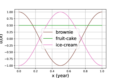
Figure 9: Alice’s true utilities for brownie, fruit cake and ice cream.

In order to infer her utility function, we ask Alice her preferences regarding the three types of desserts on 50 different days, which are randomly selected throughout the course of the year. For instance, in day $x=75/365\approx 0.2$, her preferences are $\textrm{fruit-cake}\succ\textrm{brownie}\succ\textrm{ice-cream}$ (see Figure 9). Therefore, the dataset, $\mathcal{D}_{50}$, includes a collection of fifty triplet-preferences for the three desserts, each one corresponding to each of the fifty days. We aim to learn Alice’s utility functions for the three desserts from $\mathcal{D}_{50}$ and predict her preferences for any other day of the year. Figure 10-top displays the posterior-mean of the utilities obtained from Model 4.1. It can be noticed that the the ordering between the three mean functions is in agreement with that of the original utilities (in Figure 9) for each value of $x$. Figure 10-bottom shows the posterior mean and 95% credible intervals for each of the three utilities as computed by Model 4.1.

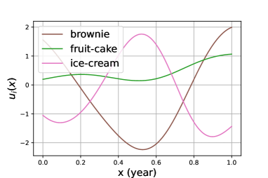
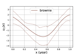
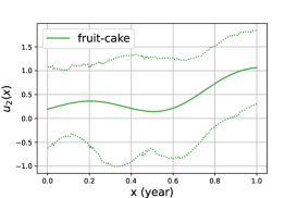
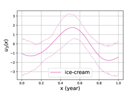
Figure 10: Top: mean of the predicted posterior utilities for the three desserts. Bottom: Predictive mean and 95% credible interval for each one of the three desserts.

If we wish to predict Alice’s preferences for the three desserts in day $x^{*}=90/365\approx 0.25$, then we can do this by computing the posterior distributions of the differences $u_{fruit-cake}-u_{brownie}$ and $u_{brownie}-u_{ice-cream}$ by sampling from the posterior. The result is shown in Figure 11. For instance, the support of the distribution for $u_{fruit-cake}-u_{brownie}>0$ does not include zero, this allows us to conclude that Alice prefers fruitcake over brownie in day $90$ with probability $\approx 1$. We are instead undecided about the comparison brownie versus ice-cream.

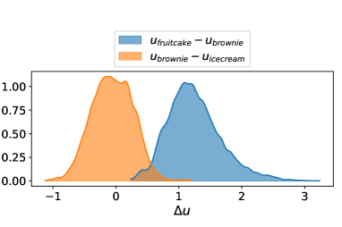
Figure 11: Posterior distributions of the differences $u_{fruitcake}-u_{brownie}$ and $u_{brownie}-u_{icecream}$.

4.2 Plackett-Luce model

Assume that, for each instance ${\bf x}^{(k)}$, we interpret a ranking of the $d$ labels as a sequence of $d-1$ independent choices, that is first Alice chooses the first item, then chooses the second among the remaining alternatives, and so on. The Plackett-Luce (PL) (Luce, 1959; Plackett, 1975) model provides a distribution over orderings. Given a dataset of orderings

$$c_{\pi^{(k)}_{1}}\succ_{{\bf x}^{(k)}}c_{\pi^{(k)}_{2}}\succ_{{\bf x}^{(k)}}c_{\pi^{(k)}_{3}}\succ_{{\bf x}^{(k)}}\dots\succ_{{\bf x}^{(k)}}c_{\pi^{(k)}_{d}},$$

for $k=1,\dots,m$, where $\bm{\pi}^{(k)}=[\pi^{(k)}_{1},\dots,\pi^{(k)}_{d}]^{\top}\in\Pi_{d}$ is a permutation of the indices $\{1,2,\dots,d\}$, the PL distribution is described in terms of the associated ordering $\bm{\pi}^{(k)}$ as

$$p(\bm{\pi}^{(k)}|{\bf a})=\prod_{i=1}^{d-1}\frac{a_{\pi^{(k)}_{i}}}{\sum_{j=i}^{d}a_{\pi^{(k)}_{j}}},$$ (43)

for $k=1,\dots,m$, where ${\bf a}\in\mathbb{R}^{d}$ with $a_{i}>0$ for $i=1,\dots,d$ are so-called score variables. This model satisfies the Luce’s axiom of Choice (Luce, 1959), which states that the odds of choosing an item over another do not depend on the set of items from which the choice is made. Indeed, for any choice $\bm{\pi}^{(k)}$ and for any two alternatives $i_{1}$ and $i_{2}$ in the choice-set ($i_{1},i_{2}\geq i$), the ratio of the probabilities is

$$\frac{\frac{a_{\pi^{(k)}_{i_{1}}}}{\sum_{j=i}^{d}a_{\pi^{(k)}_{j}}}}{\frac{a_{\pi^{(k)}_{i_{2}}}}{\sum_{j=i}^{d}a_{\pi^{(k)}_{j}}}}=\frac{a_{\pi^{(k)}_{i_{1}}}}{a_{\pi^{(k)}_{i_{2}}}},$$

which does not depend on any alternatives other than $i_{1}$ and $i_{2}$. A standard approach is to define the score $a_{i}$ as function of the utility $u_{i}$, in particular it is common to consider the relation $a_{i}=e^{u_{i}}$. In this case, the likelihood (43) becomes equal to:

$$p(\bm{\pi}^{(k)}|{\bf u}({\bf x}^{(k)}))=\prod_{i=1}^{d-1}\frac{e^{u_{i}({\bf x}^{(k)})}}{\sum_{j=i}^{d}e^{u_{j}({\bf x}^{(k)})}},$$ (44)

which is known as exploded logit likelihood model. It can be noticed that each term in the product in (44) corresponds to the softmax function used in multi-class classification.

In Model 4.2, we will use GPs to learn the utility functions underlying the PL-model.

Model 7: Plackett-Luce model for label ordering data
Consider a training dataset including the ordering of $d$-labels for each one of the $m$ covariates:

$$\mathcal{D}_{m}=\{c_{\pi^{(k)}_{1}}\succ_{{\bf x}^{(k)}}c_{\pi^{(k)}_{2}}\succ_{{\bf x}^{(k)}}c_{\pi^{(k)}_{3}}\succ_{{\bf x}^{(k)}}\dots\succ_{{\bf x}^{(k)}}c_{\pi^{(k)}_{d}}:~{}~{}\bm{\pi}^{(k)}\in\Pi_{d},{\bf x}^{(k)}\in X,~{}k=1,\dots,m\}.$$

Under the assumption that the $m$ orderings statements are conditionally independent given $\mathbf{u}(X)$, we obtain the likelihood:

$$p(\mathcal{D}_{m}|{\bf u}(X))=\prod_{k=1}^{m}\prod_{i=1}^{d-1}\frac{e^{u_{\pi_{i}^{(k)}}({\bf x}^{(k)})}}{\sum_{j=i}^{d}e^{u_{\pi_{j}^{(k)}}({\bf x}^{(k)})}}.$$ (45)

We assign independent GP priors to each utility function resulting into:

$$u_{i}\sim\mathrm{GP}(u;0,k_{i}),~{}~{}~{}~{}~{}{\bf u}=\begin{bmatrix}u_{1}\\ u_{2}\\ \vdots\\ u_{d}\\ \end{bmatrix}\sim GP\left({\bf 0},\matrixquantity[k_{1}&0&0&0\\ 0&k_{2}&0&0\\ 0&0&\ddots&0\\ 0&0&0&k_{d}]\right).$$ (46)

The posterior has not analytical form. We use a variational inference technique to learn an approximate Gaussian posterior distribution and, at the same time, infer the value of the kernels’ hyperparameters. For simplicity, we assume the same kernel $k_{i}=k_{j}$ for each utility function, although the hyperparameters can be different.

This model was proposed by Nguyen et al. (2021), who also account for ties using a threshold $\delta$ that represents the limit of discernibility. Therefore, their model integrates Model 4.2 with Model 3.2.1.

Note that, Model 4.2 can also be applied in cases where Alice only provides an ordering of a subset of the labels. Indeed, the likelihood (45) is still valid, but the inner product will include less terms. Furthermore, we can see that if Alice only states her most preferred label, the likelihood (45) and Model 4.3 simplify to the standard multiclass classification GP model. We can exploit the structure of the likelihood to reduce the number of variational parameters in the covariance matrix of the Gaussian variational distribution, similarly to what done in (Opper and Archambeau, 2009). However, in this case, the variational covariance matrix cannot be diagonal, we need some additional parameters to model the correlation between the various utilities functions.

There is a connection between Thurstone’s model and Plackett-Luce’s model. A key result by Yellott Jr (1977) states that if the variables $\widetilde{u}_{i}$ in (39) are independent, and their distributions are identical except for their means, then Thurstone’s model gives rise to a PL model if and only if the $\widetilde{u}_{i}$ are distributed according to a Gumbel distribution.

Proposition 11 (Yellott Jr (1977))

Assume that $v_{i}$ in (39) are independent variables distributed according to a Gumbel distribution, whose cumulative distribution is $p(v_{i})=e^{-e^{-v_{i}}}$, then

$$p(\widetilde{u}_{i}=\max(\widetilde{u}_{1},\dots,\widetilde{u}_{d}))=\frac{a_{i}}{\sum_{j=1}^{d}a_{j}},~{}\text{ with }~{}a_{j}=e^{u_{j}}.$$ (47)

The proof and details are reported in Appendix A. This relation is known in machine learning as the “Gumbel-max trick”.

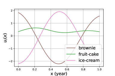
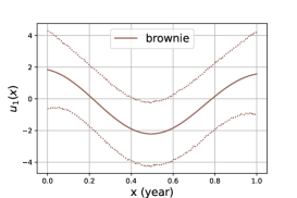
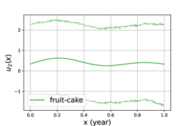
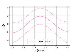
Figure 12: Top: mean of the predicted posterior utilities for the three desserts. Bottom: Predictive mean and 95% credible interval for each one of the three desserts.

Example 10

We consider the same scenario as in Example 9, where Alice orders her favourite dessert among brownie, fruit cake and ice cream on 50 different days, according to the true utilities shown in Figure 9. This results in the same dataset as in Example 9, but we interpret the triplets as orderings. Our goal is to infer Alice’s utility functions for each dessert from the dataset $\mathcal{D}_{50}$ and predict how she would order them on any other day of the year. Figure 12-top shows the posterior-mean of the utilities obtained from Model 4.1. Also in this case, it can be noticed that the the ranking between the three mean functions is in agreement with that of the original utilities. Figure 12-bottom shows the mean and 95% credible intervals for each of the three utilities separately. Since the number of possible orderings is equal to the factorial of the total number of choices (three desserts), to calculate the predicted probability of each possible ordering on a given day $x$, we can draw samples of the utilities $\mathbf{u}(x)$ from the posterior distribution and then use them to approximate ranking distribution. For this simple example, the ranking distribution at day $x=0.25$ is shown in Figure 13.

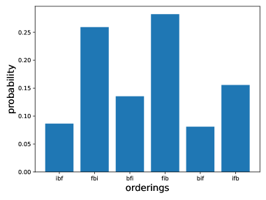
Figure 13: Predicted ranking distribution at day $x=0.25$. The string ‘ifb’ stays for icecream $\succ$ fruitcake $\succ$ brownie. The most probable ordering is ‘fib’ fruitcake $\succ$ icecream $\succ$ brownie.

4.3 Paired comparison data

Instead of asking Alice to order the $d$ labels we could ask her to choose which of each pair of labels is preferred. Thus instead of giving the ordering ($\textrm{brownie}\succ_{\bf x}\textrm{fruitcake}\succ_{\bf x}\textrm{icecream}$), she would say that, for object ${\bf x}$, “brownie is preferred to fruitcake”, “fruitcake is preferred to icecream” and “brownie is preferred to icecream”. For $d$ labels there are ${m}\choose{2}$ of such pairwise comparisons. In the following model, we assume that every time label $i$ is compared with other labels, a new utility observation $\widetilde{u}_{i}({\bf x})$ is produced, resulting in a new realisation of the noise in (39) (even for the same object ${\bf x}$). In this case, under Gaussian noise in (39), the resulting preference model is just an extension of Model 3.2.1 presented in Section 3.2.1.

Model 8: Paired comparison model with GP prior

Consider the training dataset

$$\mathcal{D}_{m}=\left\{c^{(k)}_{i}\succ_{{\bf x}^{(k)}}c^{(k)}_{j}:~{}~{}k=1,\dots,m\right\},$$ (48)

where, for each $k$, $c^{(k)}_{i}\neq c^{(k)}_{j}$, $c^{(k)}_{i},c^{(k)}_{j}\in\mathcal{C}$ and ${\bf x}^{(k)}\in\{{\bf x}_{1},{\bf x}_{2},\dots,{\bf x}_{r}\}$ with ${\bf x}_{i}\in\mathcal{X}$. Consider the vector $X=[{\bf x}_{1},{\bf x}_{2},\dots,{\bf x}_{r}]^{\top}$ and

$${\bf u}({\bf x}_{i})=\begin{bmatrix}u_{1}({\bf x}_{i})\\ u_{2}({\bf x}_{i})\\ \vdots\\ u_{d}({\bf x}_{i})\\ \end{bmatrix},~{}~{}~{}{\bf u}(X)=\begin{bmatrix}{\bf u}({\bf x}_{1})\\ {\bf u}({\bf x}_{2})\\ \vdots\\ {\bf u}({\bf x}_{d})\\ \end{bmatrix}.$$

Under the assumption that the preference statements are conditionally independent given ${\bf u}(X)$, we obtain the likelihood:

$$p(\mathcal{D}_{m}|{\bf u}(X))=\prod_{k=1}^{m}\Phi\left(u_{c^{(k)}_{i}}({\bf x}^{(k)})-u_{c^{(k)}_{j}}({\bf x}^{(k)})\right)=\Phi\left(\widetilde{W}{\bf u}(X)\right),$$ (49)

where $u_{c^{(k)}_{i}}$ (resp. $u_{c^{(k)}_{j}}$) denotes the utility function associated to the label $c^{(k)}_{i}$ (resp. $c^{(k)}_{j}$) and the last term in (49) gives the expression of the likelihood using the matrix form for a suitable $m\times(rd)$ matrix $\widetilde{W}$. We assign independent GP priors to each utility function resulting into:

$$u_{i}\sim\mathrm{GP}(u;0,k_{i}),~{}~{}~{}~{}~{}{\bf u}=\begin{bmatrix}u_{1}\\ u_{2}\\ \vdots\\ u_{d}\\ \end{bmatrix}\sim GP\left({\bf 0},\matrixquantity[k_{1}&0&0&0\\ 0&k_{2}&0&0\\ 0&0&\ddots&0\\ 0&0&0&k_{d}]\right).$$ (50)

The posterior is similar to that in (23) but with $\widetilde{W}$ instead of $W$, and the diagonal kernel in (50).

This model was first derived by Chu and Ghahramani (2005). Note that, under Gumbel noise in (39), the likelihood (49) is equal to

$$p(\mathcal{D}_{m}|{\bf u}(X))=\prod_{k=1}^{m}\frac{\exp({u_{c^{(k)}_{i}}({\bf x}^{(k)})})}{\exp({u_{c^{(k)}_{i}}({\bf x}^{(k)})})+\exp({u_{c^{(k)}_{j}}({\bf x}^{(k)})})},$$ (51)

which corresponds to a combination of Bradley and Terry model (Bradley and Terry, 1952) and Babington Smith model (Smith, 1950) proposed by (Mallows, 1957).

In order to understand the difference between the above pairwise comparison model and the previous two models consider the preferences: $\textrm{brownie}\succ_{\bf x}\textrm{fruitcake}$ and $\textrm{fruitcake}\succ_{\bf x}\textrm{icecream}$. Under the independence assumption underlying the likelihood (49) and Gaussian noise, these preferences imply the utility relations:

1. first preference: $u_{\textrm{brownie}}+v_{\textrm{brownie}}>u_{\textrm{fruitcake}}+v_{\textrm{fruitcake}}$;

2. second preference: $u_{\textrm{fruitcake}}+v^{\prime}_{\textrm{fruitcake}}>u_{\textrm{icecream}}+v_{\textrm{icecream}}$;

where $v_{\textrm{fruitcake}},v^{\prime}_{\textrm{fruitcake}}$ are two different realisations of the noise. Therefore, we cannot invoke the transitive property to conclude that $\textrm{brownie}\succ_{\bf x}\textrm{icecream}$ (and, in general, Model 4.3 will not predict that). Therefore, Model 4.3 should only be applied when the pairwise comparisons are independent, otherwise the posterior will be incorrect, as similarly shown in Example 7.

5 Choice functions

In the previous sections, we have assumed that Alice expresses her judgements either as preferences or as an ordering. However, we often only observe her choices. For instance, given a set of products on an internet commerce site, she may decide to click on/buy some of them.

Mathematically, Alice’s choices can be formalised through the concept of choice functions. Let $\mathcal{Q}$ denote the set of all finite subsets of $\mathcal{X}$ (or $\mathcal{C}$ for label preference).

Definition 12

A choice function $C$ is a set-valued operator on sets of options. More precisely, it is a map $C:\mathcal{Q}\rightarrow\mathcal{Q}$ such that, for any set of options $A\in\mathcal{Q}$, the corresponding value of $C$ is a subset $C(A)$ of $A$ (see for instance Kreps et al. (1990)).

It will be assumed throughout this paper that Alice is able to find a choosable option in every set she is presented with, and therefore $C(A)\neq\emptyset$ for all $A$. It is convenient to introduce the set of rejected options, denoted by $R(A)$, and equal to $A\backslash C(A)$.

Example 11

Let’s explore another example where we seek to model Alice’s preferences among various types of cupcake. We assume that the differences between these cupcake types is determined by their recipe. In the context of choice modelling, our primary goal is on observing Alice’s choices among the various cupcake options, without delving into the specifics of how her preferences are determined. To be more specific, we present Alice with a set of different cupcakes, each one prepared with a different recipe that defines its characteristics, and ask her to pick the ones that appeal to her the most. Like for example, given the choice set $A=$$\bigg{\{}$ , , , $\bigg{\}}$, she chooses

$C(A)=$$\bigg{\{}$ , $\bigg{\}}$ and, therefore, she rejects $R(A)=$$\bigg{\{}$, $\bigg{\}}$.

There are two main interpretations of choice functions. In both interpretations, for a given option set $A\in\mathcal{Q}$, the statement that an option $o_{j}\in A$ is rejected from $A$ (that is, $o_{j}\notin C(A)$) means that there is at least one option $o_{i}\in A$ that a subject prefers over $o_{j}$. Alice is not required to tell us which option(s) in $C(A)$ she prefers to $o_{j}$. This makes choice functions a very easy-to-use tool to express choices.

The two interpretations differ instead in the meaning of the statement $o_{i}\in C(A)$.

1. In the traditional interpretation, one reads the statement $o_{i}\in C(A)$ as “$o_{i}$ is considerate to be at least as good as all other options in $A$,” and thus infers from a statement like $\{o_{i},o_{j}\}\subseteq C(A)$ that Alice is indifferent between $o_{i}$ and $o_{j}$.

2. The alternative and more general interpretation of $\{o_{i},o_{j}\}\subseteq C(A)$ is that $o_{i}$ and $o_{j}$ are incomparable for Alice. Equivalently, $\{o_{i},o_{j}\}\subseteq C(A)$ should be read as “$o_{i}$ and $o_{j}$ are undominated in $A$” (in a sense that will be clarified hereafter).

Example 12

For simplicity, we only consider a single ingredient for the cupcakes, denoted as $x\in[0,1]$. For instance, $x$ may be the normalised amount of butter. We present Alice with sets of different cupcakes (only differing in the amount of butter) and asks Alice to taste them and pick up her favourite ones.

$$A_{1} =\{0,0.25,0.5\}, C(A_{1}) =\{0.25,0.5\},$$

$$A_{2} =\{0.4,0.5,0.6\}, C(A_{2}) =\{0.4,0.5,0.6\},$$

$$A_{3} =\{0,0.1,0.2\}, C(A_{3}) =\{0.2\}.$$

It can be noted that there are cases where she chooses more than one cupcake. This may happen because she is considering different characteristics of the object, such as taste and softness. This may also happen because she is uncertain about her choices, for instance because she is selecting cupcakes to share with a group of friends (in economics this problem is referred to multiple-self decision making). From a machine learning perpsective, our goal is to learn a model that allows us to predict Alice’s choices for the different set of cupcakes $A^{*}=\{x_{a}^{*},x_{b}^{*},x_{c}^{*}\}$.

5.1 Consistency of choice functions

In Section 2.1, we have discussed the properties that a preference relation should have to be considered consistent. There are three important properties for choice functions (Chernoff, 1954; Sen, 1971; Aizerman and Malishevski, 1981; Moulin, 1985; Schwartz, 1986).

The first property states that if an object is selected from a set of alternatives $A$, it should also be selected in any subset $A^{\prime}$ that contains it.

Chernoff:

if $A^{\prime}\subset A$ then $(C(A)\cap A^{\prime})\subset C(A^{\prime})$.

The second property states that every object that is selected from two different sets $A,A^{\prime}$ should also be selected from their union $A\cup A^{\prime}$.

Expansion:

$\forall A,A^{\prime}$,  $(C(A)\cap C(A^{\prime}))\subset C(A\cup A^{\prime})$.

The third property states that the subset of objects chosen from a set cannot expand when non selected objects are removed from that set.

Aizerman:

$\forall A,A^{\prime}$, if $C(A)\subset A^{\prime}\subset A$ then $C(A^{\prime})\subset C(A)$.

Chernoff and Expansion are also known as $\alpha$ and $\gamma$ consistency rules. Similarly to what was done for preferences, we can ask if a consistent choice function defines/it is defined by some utility functions. We first introduce to concept of Pareto rationalisability.

Definition 13 (Pareto rationalisability)

Given a collection of strict orders $\{\succ_{k}\}_{k=1}^{d}$, they are said to Pareto rationalise $C$ when the following condition holds:

$\forall A\in\mathcal{Q}$, $\forall o_{i}\in A$, $o_{i}\in C(A)$ if and only $\nexists o_{j}\in A$ such that $o_{j}\succ_{k}o_{i}$ $\forall k\in\{1,2\dots,d\}$.

Pareto Rationalisability means that only the objects that are not dominated by any other objects in the same set are chosen.

Proposition 14 (Moulin (1985))

Let $C:\mathcal{Q}\rightarrow\mathcal{Q}$ be a choice function. There exists a set of strict preferences $\{\succ_{k}\}_{k=1}^{d}$ that Pareto rationalises $C$ if and only if $C$ satisfies Chernoff, Expansion and Aizerman.

As discussed in Section 2.1, any strict order $\succ_{i}$ can be represented by a utility function $u_{i}$ and vice versa. Proposition 14 tells us that there is a latent vector of utility functions ${\bf u}(o)=[u_{1}(o),\dots,u_{d}(o)]^{\top}$, for some finite dimension $d$, which represents the choice function $C$ if and only if $C$ satisfies Chernoff, Expansion and Aizerman. ${\bf u}$ embeds the options $o$ into a space $\mathbb{R}^{d}$ and the choice set $C(A)$ expresses a Pareto set of strongly undominated options with respect the utilities ${\bf u}$.

We may question if Chernoff, Expansion and Aizerman are always desirable properties. Thinking in terms of a vector of utilities, we may think of situations where Alice, in case of options with conflicting quality attributes (utilities), might pick those options that are optimal for at least one of these attributes. Then, this way of choosing is called pseudo-rational.

Proposition 15 (Moulin (1985))

A choice function is pseudo-rationalisable if and only if it satisfies Chernoff and Aizerman.

Pseudo-rationalisability is a weaker property than Pareto rationalisability. It represents a choice function in the form

$$C(A)=\bigcup\limits_{k=1,\dots,d}\arg\max_{o\in A}u_{k}(o),$$ (52)

and, therefore, it requires less rationality (less consistency of the choice sets) than representing it in the Pareto sense.

5.2 Learning rational and pseudo-rational choice functions

We will start with Pareto rational choice functions. For each $A$, we interpret $C(A)$ as the undominated set in the strong Pareto sense, with $R(A)$ being the set of dominated options. We consider a latent vector of utility functions ${\bf u}({\bf o})=[u_{1}({\bf o}),\dots,u_{d}({\bf o})]^{\top}$, which embeds the objects ${\bf o}$ into a space $\mathbb{R}^{d}$. We say that an object ${\bf o}\in A$ is not dominated by an object ${\bf v}$ if

$$\min_{i\in\{1,\ldots,d\}}(u_{i}({\bf o})-u_{i}({\bf v}))>0,$$ (53)

that is all utilities $u_{i}$ take a larger value at ${\bf o}$ than at ${\bf v}$.

The choice set can then be represented through a Pareto set of strongly undominated options:

$$\neg \left(\min_{i\in\{1,\dots,d\}}(u_{i}({\bf o})-u_{i}({\bf v}))\leq 0,~{}~{}\forall{\bf o}\in C(A)\right),~{}~{}\forall{\bf v}\in R(A),$$ (54)

$$\min_{i\in\{1,\dots,d\}}(u_{i}({\bf o})-u_{i}({\bf v}))\leq 0,~{}\forall{\bf o},{\bf v}\in C(A),~{}~{}{\bf o}\neq{\bf v}.$$ (55)

The first condition, in (54), means that, for each option ${\bf v}\in R(A)$, it is not true ($\neg$ stands for logical negation) that all options in $C(A)$ are no-better than ${\bf v}$. In particular, there is at least an option in $C(A)$ which is better than ${\bf v}$. Condition (55) means that, for each option in $C(A)$, there is no better option in $C(A)$. This requires that the latent functions values of the options should be consistent with the choice function implied relations.

To account for possible violations of rationality, similarly to what done in Model (3.2.1), we replace the hard-constraints (54)–(55) with soft-constraints defining a likelihood model. In particular, consider the dataset

$$\mathcal{D}_{m}=\{(A_{k},C(A_{k})):\text{ for }k=1,\dots,m\},$$

given the latent vector function ${\bf u}$, the likelihood is

$$p(\mathcal{D}_{m}|{\bf u}(X))=\prod_{k=1}^{m}p(C(A_{k}),A_{k}|{\bf u}(X)),$$ (56)

with

$$p(C(A_{k}),A_{k}|{\bf u}(X)) =\prod\limits_{\{{\bf o},{\bf v}\}\in C_{\sharp}(A_{k})}\Bigg{(}1-\prod_{i=1}^{d}\Phi\left(\frac{u_{i}({\bf o})-u_{i}({\bf v})}{\sigma}\right)-\prod_{i=1}^{d}\Phi\left(\frac{u_{i}({\bf v})-u_{i}({\bf o})}{\sigma}\right)\Bigg{)}$$ (57)

$$\prod_{{\bf v}\in R(A_{k})}\Bigg{(}1-\prod_{{\bf o}\in C(A_{k})}\left(1-\prod_{i=1}^{d}\Phi\left(\frac{u_{i}({\bf o})-u_{i}({\bf v})}{\sigma}\right)\right),$$

where the notation $\{{\bf o},{\bf v}\}\in C_{\sharp}(A_{k})$ means that the pair $\{{\bf o},{\bf v}\}$ is an element of $C_{\sharp}(A_{k})$, which denotes the set of all possible 2-combination (without repetition) of the elements of the set $C(A_{k})$. We assumed that the choice-statements $k=1,\dots,m$ are conditionally independent given the utilities ${\bf u}(X)$, which is in line with our model based on Pareto rationalisation. The product in the first and second row in (57) is a probabilistic relaxation of (55). Note the negation $1-\prod_{i=1}^{d}\Phi\left(\frac{u_{i}({\bf o})-u_{i}({\bf v})}{\sigma}\right)-\prod_{i=1}^{d}\Phi\left(\frac{u_{i}({\bf v})-u_{i}({\bf o})}{\sigma}\right)$, which states that ${\bf o}$ does not dominate ${\bf v}$ and vice versa. The product in the last row in (57) is a probabilistic relaxation of (54).

Example 13 (Inspired by example 1 in Benavoli et al. (2023a))

To understand the likelihood (57), let us consider four objects ${\bf o}_{1},{\bf o}_{2},{\bf o}_{3},{\bf o}_{4}$ and the utilities:

$${\bf u}({\bf o}_{1})=\begin{bmatrix}0.2\\ 0\end{bmatrix},{\bf u}({\bf o}_{2})=\begin{bmatrix}0.1\\ 0.2\end{bmatrix},{\bf u}({\bf o}_{3})=\begin{bmatrix}-1\\ -1\end{bmatrix},{\bf u}({\bf o}_{4})=\begin{bmatrix}-0.5\\ -0.5\end{bmatrix}.$$

The objects $\{{\bf o}_{1},{\bf o}_{2}\}$ are hard to tell apart since they have very similar utilities. For this reason, Alice may make mistakes when comparing them. For instance, she makes the following choices:

$$C(\{{\bf o}_{1},{\bf o}_{2},{\bf o}_{3}\})=\{{\bf o}_{1},{\bf o}_{2}\},~{}~{}C(\{{\bf o}_{1},{\bf o}_{2},{\bf o}_{4}\})=\{{\bf o}_{1}\}.$$

Those choices are not Pareto rationalisable according to the order induced by the utility functions above. In particular, this implies that conditions (54)–(55) are not simultaneously satisfied. On the other hand, the likelihood (57) is not zero on this dataset, because it accounts for errors in Alice’s choices. Assuming $\sigma=1$, the likelihood for the two choices is

$${}p(\{{\bf o}_{1},{\bf o}_{2}\},\{{\bf o}_{1},{\bf o}_{2},{\bf o}_{3}\}|{\bf u}(X)) \approx 0.48,$$

$$p(\{{\bf o}_{1}\},\{{\bf o}_{1},{\bf o}_{2},{\bf o}_{4}\}|{\bf u}(X)) \approx 0.12.$$

This means that, for the above latent utilities, the probability that Alice jointly makes these choices is $0.48\cdot 0.12=0.057$. Note that, the probability of error increases with the parameter $\sigma$. Indeed, the probability $p(\{{\bf o}_{1},{\bf o}_{2}\},\{{\bf o}_{1},{\bf o}_{2},{\bf o}_{3}\}|{\bf u}(X))p(\{{\bf o}_{1}\},\{{\bf o}_{1},{\bf o}_{2},{\bf o}_{4}\}|{\bf u}(X))$ tends to zero for $\sigma\rightarrow 0$, since in this case the likelihood (57) reduces to (54)–(55) and Alice’s choice is Pareto irrational.

We will now move to pseudo-rationalisable choice functions. In this case, we say that an object ${\bf o}\in A$ is not dominated by an object ${\bf v}$ if:

$$\max_{i\in\{1,\ldots,d\}}(u_{i}({\bf o})-u_{i}({\bf v}))>0,$$ (58)

that is, there is a utility where object ${\bf o}$ is better than ${\bf v}$. The choice set is then represented through the following conditions:

$$\left(\forall i\in\{1,\dots,d\}~{}~{}\neg\left(\min_{{\bf o}\in C(A)}(u_{i}({\bf v})-u_{i}({\bf o}))\geq 0\right)\right),~{}~{}\forall v\in R(A),$$ (59)

$$\min_{i\in\{1,\dots,d\}}(u_{i}({\bf o})-u_{i}({\bf v}))\leq 0,~{}\forall{\bf o},{\bf v}\in C(A),~{}~{}{\bf o}\neq{\bf v},$$ (60)

where condition (59) means that for all ${\bf v}\in R(A)$, it is not true that the value of any latent function in ${\bf v}$ is higher than their value in any ${\bf o}\in C(A)$. Condition (60) instead imposes that each object in $C(A)$ is not dominated according to (58). By using the same technique used above to relax the constraints we obtain the likelihood $p(\mathcal{D}_{m}|{\bf u}(X))=\prod_{k=1}^{m}p(C(A_{k}),A_{k}|{\bf u}(X))$ with:

$$p(C(A_{k}),A_{k}|{\bf u}(X)) =\prod\limits_{\{{\bf o},{\bf v}\}\in C_{\sharp}(A_{k})}\Bigg{(}1-\prod_{i=1}^{d}\Phi\left(\frac{u_{i}({\bf o})-u_{i}({\bf v})}{\sigma}\right)-\prod_{i=1}^{d}\Phi\left(\frac{u_{i}({\bf v})-u_{i}({\bf o})}{\sigma}\right)\Bigg{)}$$ (61)

$$\prod_{{\bf v}\in R(A_{k})}\Bigg{(}\prod_{i=1}^{d}\left(1-\prod_{{\bf o}\in C(A_{k})}\Phi\left(\frac{u_{i}({\bf v})-u_{i}({\bf o})}{\sigma}\right)\right).$$

Note that the first part of (61) remains the same as in the rational case, however the second part now enforces the dominance defined in (58).

Example 14

To understand the above likelihood, let us consider again four objects ${\bf o}_{1},{\bf o}_{2},{\bf o}_{3},{\bf o}_{4}$ and the utilities:

$${\bf u}({\bf o}_{1})=\begin{bmatrix}0.2\\ -1.5\end{bmatrix},{\bf u}({\bf o}_{2})=\begin{bmatrix}-1.5\\ 0.2\end{bmatrix},{\bf u}({\bf o}_{3})=\begin{bmatrix}-1\\ -1\end{bmatrix},{\bf u}({\bf o}_{4})=\begin{bmatrix}-2\\ -2\end{bmatrix}.$$

Assume Alice makes the following choices:

$$C(\{{\bf o}_{1},{\bf o}_{2},{\bf o}_{3}\})=\{{\bf o}_{1},{\bf o}_{2}\},~{}~{}C(\{{\bf o}_{1},{\bf o}_{2},{\bf o}_{4}\})=\{{\bf o}_{1},{\bf o}_{2}\}.$$

Those choices are not Pareto rationalisable, but they are Pareto pseudo-rationalisable according to the order induced by the utility functions above. In particular, this implies that conditions (54)– (55) are not simultaneously satisfied, while this is the case for (59)–(60). Indeed, for $\sigma=1$, the likelihood (61)

$$p(\{{\bf o}_{1},{\bf o}_{2}\},\{{\bf o}_{1},{\bf o}_{2},{\bf o}_{3}\}|{\bf u}(X)) \approx 0.77,$$

$$p(\{{\bf o}_{1},{\bf o}_{2}\},\{{\bf o}_{1},{\bf o}_{2},{\bf o}_{4}\}|{\bf u}(X)) \approx 0.91.$$

and their product is $0.77\cdot 0.91\approx 0.71$, while the likelihood (57) is equal to

$${}p(\{{\bf o}_{1},{\bf o}_{2}\},\{{\bf o}_{1},{\bf o}_{2},{\bf o}_{3}\}|{\bf u}(X)) \approx 0.43,$$

$$p(\{{\bf o}_{1},{\bf o}_{2}\},\{{\bf o}_{1},{\bf o}_{2},{\bf o}_{4}\}|{\bf u}(X)) \approx 0.82.$$

and their product is $0.43\cdot 0.82=0.35$. For $\sigma\rightarrow 0$, the two products converge to $1$ and, respectively $0$. This holds because Alice’s choices are pseudo-rationalisable but not Pareto rationalisable.

Model 9: Rational and Pseudo-rational models for choice data
Consider the training dataset:

$$\mathcal{D}_{m}=\{(A_{k},C(A_{k})):\text{ for }k=1,\dots,m\},$$ (62)

where, for each $k$, $\emptyset\neq C(A_{k})\subseteq A_{k}$ and $A_{k}\subset\{{\bf x}_{1},{\bf x}_{2},\dots,{\bf x}_{r}\}$ with ${\bf x}_{i}\in\mathcal{X}$. Consider the vector $X=[{\bf x}_{1},{\bf x}_{2},\dots,{\bf x}_{r}]^{\top}$ and

$${\bf u}({\bf x}_{i})=\begin{bmatrix}u_{1}({\bf x}_{i})\\ u_{2}({\bf x}_{i})\\ \vdots\\ u_{d}({\bf x}_{i})\\ \end{bmatrix},~{}~{}~{}{\bf u}(X)=\begin{bmatrix}{\bf u}({\bf x}_{1})\\ {\bf u}({\bf x}_{2})\\ \vdots\\ {\bf u}({\bf x}_{d})\\ \end{bmatrix}.$$

Under the assumption that the choice statements are conditionally independent given ${\bf u}(X)$, we obtain the likelihood:

$$p(\mathcal{D}_{m}|{\bf u}(X)) =\prod_{k=1}^{m}p(C(A_{k}),A_{k}|{\bf u}(X))~{}~{}\text{ with }$$ (63)

$$p(C(A_{k}),A_{k}|{\bf u}(X)) =\left\{\begin{array}[]{ll}\text{\eqref{eq:likelihoodexpanse00}}&\text{for rational choices}\\ \text{\eqref{eq:likelihoodpseudorat}}&\text{for pseudo-rational choices}\end{array}\right.$$

We assign independent GP priors to each utility function resulting into:

$$u_{i}\sim\mathrm{GP}(u;0,k_{i}),~{}~{}~{}~{}~{}{\bf u}=\begin{bmatrix}u_{1}\\ u_{2}\\ \vdots\\ u_{d}\\ \end{bmatrix}\sim GP\left({\bf 0},\matrixquantity[k_{1}&0&0&0\\ 0&k_{2}&0&0\\ 0&0&\ddots&0\\ 0&0&0&k_{d}]\right).$$ (64)

The posterior is approximated using variational inference.

Note that, Model 5.2 comprises two distinct models depending on the selected likelihood. The derivation of the likelihood (61) is based on less assumptions regarding the choice functions, making it more general. However, it is less informative in applications where the subject’s choices are based on Pareto rationalisation. In this case, it is better to use (57). Learning Rationalisable choice functions via a Pareto embedding was originally proposed by Pfannschmidt and Hüllermeier (2020), but using a hinge-loss and a neural network based model. The GP model was derived in Benavoli et al. (2023a). Recently, Pfannschmidt et al. (2022) have extended their work to learn context-based choices. This framework deals with situations in which a subject’s choices are context-dependent, which means that the preference in favour of a certain choice alternative may depend on what other options are also available in the choice-set. In general, these models reject the Chernoff-axiom (Tversky and Simonson, 1993).

In Model 5.2, we have assumed that the number of latent utilities is fixed/known. Model 5.2 works well if the number of latent functions in the model is greater than equal of the number implicit criteria that Alice uses to make her choices. If this upper bound is unknown, a way to learn the number of utility functions is through the Leave-One-Out cross-validation score, which can be computed from the posterior distribution (Benavoli et al., 2023a).

Example 15

We consider a scenario as in Example 9, where Alice chooses her favourite cupcakes from given choice-sets (where the cupcakes differ for the amount of butter). We assume her choices are Pareto-rational and determined by the two latent utilities shown in Figure 14.

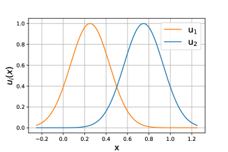
Figure 14: True latent utilities function that underlay Alice’s Pareto-rational choices.

We use these utilities ${\bf u}=[u_{1},u_{2}]^{\top}$ to define a choice function via Pareto dominance. For instance, consider the set of options $A=\{x_{1},x_{2},x_{3}\}$, assume that ${\bf u}(x_{1})=[1,0.05]$, ${\bf u}(x_{2})=[0.5,0]$, ${\bf u}(x_{3})=[0.05,1]$, we have that $C(A)=\{x_{1},x_{3}\}$ and $R(A)=A\backslash C(A_{k})=\{x_{2}\}$. In fact, one can notice that $[1,0.05]$ dominates $[0.5,0]$ on both the utilities, and $[1,0.05]$ and $[0.05,1]$ are incomparable. We sample $60$ inputs $x_{i}$ at random in $[-0.25,1.25]$ and, using the above approach, we generated a dataset of $m=200$ random subsets $\{A_{k}\}_{k=1}^{m}$ of the $60$ points each one of size $|A_{k}|=3$ and compute the corresponding choice pairs $(C(A_{k}),A_{k})$ based on ${\bf u}$.

Our goal is to infer Alice’s utility functions from the dataset $\mathcal{D}_{200}$ and predict her choices.

Figure 15-left shows the posterior-mean of the utilities and 95% credible intervals for the learned two utility functions. It can be noticed that the learned utilities are in agreement with the true ones in Figure 14. Figure 15-right shows 5 samples of the two utilities from the posterior. These samples are correlated – they always cross near the middle. This happens because the variational posterior captures the relative difference between the two utilities that determines the Pareto-based choices (modelled through the likelihood (57)).

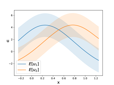
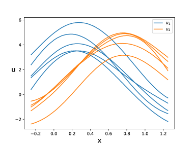
Figure 15: Learned utilities from rational choice data using Model 5.2 with rational likelihood. Left: mean and credible region of the predicted posterior utilities. Right: a sample from the posterior.

We have repeated this experiment generating pseudo-rational choices and then used the rational-likelihood and, respectively, pseudo-rational-likelihood based model to learn back the utilities. The posterior in the two cases are shown in Figure 16 and, respectively, 17. In Figure 16, it can be noticed that the relative difference between the two expected utilities and the posterior samples is wrong. They do not cross in the middle of the interval $[-0.25,1.25]$. This holds because the data are not Pareto rational and the learned model is therefore “biased”. Figure 17 shows instead that the pseudo-rational model is able to correctly learn the utilities.

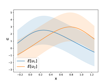
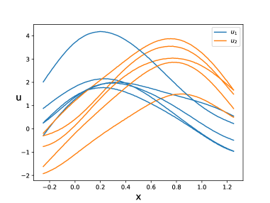
Figure 16: Learned utilities from pseudo-rational choice data using Model 5.2 with rational likelihood. Left: mean and credible region of the predicted posterior utilities. Right: 5 samples from the posterior.

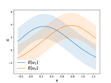
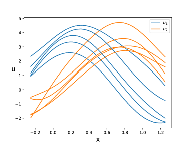
Figure 17: Learned utilities from pseudo-rational choice data using Model 5.2 with pseudo-rational likelihood. Left: mean and credible region of the predicted posterior utilities. Right: 5 samples from the posterior.

6 Applications

Hereafter, we will apply the models introduced earlier to real datasets.

6.1 Transportation mode preference

First, we consider a dataset including the choices made by subjects regarding their preferred transport mode for the Montreal-Toronto corridor (Forinash and Koppelman, 1993; Croissant, 2020). There are four transport modes (air, bus, car and train) and we have the following information about the journey: dist the distance of the trip, cost the monetary cost, ivt the in-vehicle-time, ovt the out-of-vehicle time, freq the frequency and noalt the number of available alternatives. There are also subject specific variables: income the household income and urban an indicator variable for trips which have a large city at the origin or the destination. Table 1 shows a subset of the dataset. Each case corresponds to a different choice set for an individual. The dataset includes 4221 different transport modes and 4322 cases (leading to 15520 rows). This dataset will allow us to explore how the various models we have previously introduced can be applied to address diverse choice tasks.

case	alt	choice	dist	cost	ivt	ovt	freq	income	urban	noalt
129	train	0	387	58.25	316	59	2	55	0	4
129	air	0	387	145.80	56	85	9	55	0	4
129	bus	0	387	26.67	301	58	8	55	0	4
129	car	1	387	73.53	251	0	0	55	0	4
130	train	0	387	58.25	316	59	2	45	0	4
130	air	0	387	145.80	56	85	9	45	0	4
130	bus	0	387	26.67	301	58	8	45	0	4
130	car	1	387	73.53	251	0	0	45	0	4
131	train	0	404	60.25	316	74	2	70	0	4
131	air	0	404	146.20	56	94	9	70	0	4
131	bus	0	404	26.67	301	93	8	70	0	4
131	car	1	404	76.76	265	0	0	70	0	4
132	train	1	365	60.85	237	94	4	70	1	4
132	air	0	365	151.20	56	77	9	70	1	4
132	bus	0	365	27.82	301	83	8	70	1	4
132	car	0	365	69.35	245	0	0	70	1	4

Table 1: Each case is a different choice task.

We will only focus on the subset of the choices with noalt=4, namely those for which four transportation modes are available. In Table 1, we can see four cases belonging to this subset. For instance in case $129$, a subject (income=55, urban=0) selected the car-mode (with features dist=387, cost=73.53, ivt=251, ovt=0, freq=0). In this first analysis, we will disregard subject-specific variables (income and urban), approaching the problem as an object-preference problem. Therefore, we will select the subset of subjects with income=70 and urban=1 (a total of $679$ cases). Since subjects make always a transportation-mode choice, instances where the same individuals select both transportation modes cannot occur. In simpler terms, we will not observe instances of indifference (for instance if several transportation modes have closely ranked utilities for the subject), nor will we observe cases of incompatibility (where a subject makes both choices).

In this first analysis, we will interpret a choice, for instance car, as the set of binary preferences over the covariates of the transportation modes, that is ${\bf x}_{car}\succ{\bf x}_{air}$, ${\bf x}_{car}\succ{\bf x}_{bus}$, ${\bf x}_{car}\succ{\bf x}_{train}$. We will assume independent pairwise comparisons and use Model 3.2.1 (which is equivalent to Model 3.2.3 under independent noises). We first consider a linear utility in the covariates:

$$u({\bf x})=\beta_{1}\texttt{dist}+\beta_{2}\texttt{cost}+\beta_{3}\texttt{ivt}+\beta_{4}\texttt{ovt}+\beta_{5}\texttt{freq},$$ (65)

with ${\bf x}=[\texttt{dist},\texttt{cost},\texttt{ivt},\texttt{ovt},\texttt{freq}]^{\top}$, but we estimate the unknown coefficients $\beta_{i}$ through Bayesian inference under the independent priors $\beta_{i}\sim N(0,\sigma_{i}^{2})$. Note that, for any two objects ${\bf x},{\bf x}^{\prime}$, we have that $E[u({\bf x})]=E[u({\bf x}^{\prime})]=0$ and

$$E[u({\bf x})u({\bf x}^{\prime})]=k({\bf x},{\bf x}^{\prime})=\sum_{i=1}^{5}\sigma^{2}_{i}x_{i}x^{\prime}_{i},$$ (66)

which is know as linear kernel. Therefore, using the kernel (66), Model 3.2.1 is equivalent to a classical Bayesian linear utility model with Probit likelihood. In Model 3.2.1, the variances $\sigma^{2}_{i}$ are inferred by maximising the marginal likelihood computed by using the Laplace’s approximation. The estimated variances for the training data (after standardising the data) are:

$$\sigma^{2}_{\texttt{dist}}\approx 0.14,~{}\sigma^{2}_{\texttt{cost}}\approx 0.085,~{}\sigma^{2}_{\texttt{ivt}}\approx 1.54,~{}\sigma^{2}_{\texttt{ovt}}\approx 0.33,~{}\sigma^{2}_{\texttt{freq}}\approx 0,$$

which highlights that the most important features are ivt,ovt and dist. By randomly splitting the dataset in 70% training and 30% testing ($10$ repetitions), we computed the model’s predictive accuracy for subjects’ choices in the test set: 84.3%. For one of the splitting, we reported the posterior predicted utilities, in Figure 18 (left), for the transportation modes (in the testing set) listed in Table 2. Assume, for instance, that we wish to predict the effect of a reduction of the ivt for the train to $30$ minutes with an increasing in cost to $50$. Figure 18 (right) shows that car and the new train transportation mode have now similar utilities.

alt	dist	cost	ivt	ovt	freq
bus	175	18.43	119	75	4
car	175	33.25	115	0	0
train	175	38.15	109	65	5
air	175	155.90	60	118	6

Table 2: Four transportation modes

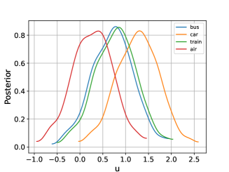
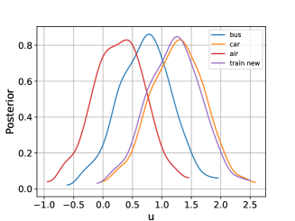
Figure 18: Predicted utilities for the Transportation modes in Table 2 for the linear kernel (left). The right plot shows the predicted utility for a new transportation mode.

The advantage of working with GPs is that we can move from linear to nonlinear utility in the covariates by simply changing the kernel. For instance, we have considered the Square-Exponential kernel:

$$E[u({\bf x})u({\bf x}^{\prime})]=k({\bf x},{\bf x}^{\prime})=\sigma^{2}e^{-\sum_{i=1}^{5}\frac{(x_{i}-x_{i}^{\prime})^{2}}{2\ell_{i}^{2}}},$$ (67)

and estimated (after standardising the data) its $6$ hyperparameters.

$$\ell_{\texttt{dist}}\approx 0.94,~{}\ell_{\texttt{cost}}\approx 0.49,~{}\ell_{\texttt{ivt}}\approx 4.1,~{}\ell_{\texttt{ovt}}\approx 1.31,~{}\ell_{\texttt{freq}}\approx 0.52,~{}\sigma^{2}=3.8,$$

which highlights that the most important features (small means more important) are cost, freq, dist and ovt. By randomly splitting the dataset in 70% training and 30% testing ($10$ repetitions), we computed the model’s predictive accuracy for subjects’ choices in the test set: 90%. This is considerably higher than the accuracy of the linear model. Figure 19 (left) shows the posterior predicted utilities for the transportation modes in Table 2, and Figure 19 (right) reports the posterior for the new train transportation mode.

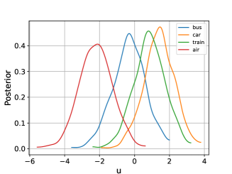
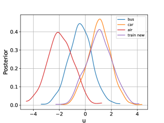
Figure 19: Predicted utilities for the Transportation modes in Table 2 for the SE kernel (left). The right plot shows the predicted utility for a new transportation mode.

Finally, instead of interpreting a choice as the set of binary preferences over the covariates of the other transportation modes (example: ${\bf x}_{car}\succ{\bf x}_{air}$, ${\bf x}_{car}\succ{\bf x}_{bus}$, ${\bf x}_{car}\succ{\bf x}_{train}$), we could directly consider choice functions $A=\{{\bf x}_{air},{\bf x}_{bus},{\bf x}_{car},{\bf x}_{train}\}$ and $C(A)=\{{\bf x}_{car}\}$ using Model 5.2. However, since each subject always selects a single transportation mode, this model is equivalent to Model 3.2.1. Table 3 summarises the accuracy results.

	Model 3.2.1 Linear Kernel	Model 3.2.1 SE Kernel	Model 5.2 SE Kernel
Accuracy	0.84	0.90	0.90

Table 3: Prediction accuracy for the transportation dataset.

There are various approaches to incorporating the subjects’ covariates income,urban into this analysis and join preference data from different Income groups. For example, in the SE kernel, one could employ distinct variance parameters for each income group (using instead the same lengthscales across groups). In light of the interpretation of Model 3.2.1, this would suggest that individuals belonging to different income groups may have varying notions of close-utility. We considered preference data from three income groups (with incomes of $35,45,55$, all having similar dataset sizes) and assessed the performance of Model 3.2.1 using a block diagonal SE kernel. Each income group had its own block, sharing a common lengthscale but with either shared variance or different variance parameter. The predictive accuracy achieved were 86% and 88%, respectively.

6.2 Ranked data for gaming platforms

For label-preference, we consider the results of a survey among 91 Dutch students (Fok et al., 2012). This survey considered the purchase of a new gaming platform and students were required to rank six options: the Xbox, PlayStation, GameCube, PlayStation Portable, Game Boy, and a regular PC. Additionally, we know (1) their age; (2) which of the 6 platforms the student owns; (3) the average number of hours that each student spends on gaming each week. As an example, the results of the survey for three students with age 33, 19 and 18 is shown in Table 4.

age	hours	platform	choice	own	choceid
33	2.00	GameBoy	6	0	1
33	2.00	GameCube	5	0	1
33	2.00	PC	4	1	1
33	2.00	PlayStation	1	1	1
33	2.00	PSPortable	3	0	1
33	2.00	Xbox	2	0	1
19	3.25	GameBoy	6	0	2
19	3.25	GameCube	5	0	2
19	3.25	PC	1	1	2
19	3.25	PlayStation	2	1	2
19	3.25	PSPortable	3	0	2
19	3.25	Xbox	4	0	2
18	4.00	GameBoy	6	0	3
18	4.00	GameCube	4	0	3
18	4.00	PC	5	1	3
18	4.00	PlayStation	1	1	3
18	4.00	PSPortable	2	0	3
18	4.00	Xbox	3	0	3

Table 4: Dataset: ranked data for gaming platforms

Since these are ranked data, we can use Model 4.2 to predict their ranking. There are 6 different labels (Xbox, PlayStation, GameCube, PlayStation Portable, Game Boy) and the subject’s covariates are age, hours and own. For instance, for the first subject (age=33, hours=2, own=$\{$PC,PlayStation$\}$) in Table 4, the ranking is PlayStation, Xbox, PlayStation Portable, PC, GameCube and Game Boy. Given the covariates of a subject

$${\bf x}=[\texttt{ownGameBoy},\texttt{ownGameCube},\texttt{ownPC},\texttt{ownPlayStation},\texttt{ownPSPortable},\texttt{ownXbox},\texttt{age},\texttt{hours}],$$

the goal is to learn their gaming platforms ranking. This can be accomplished by learning the utilities

$${\bf u}({\bf x})=[u_{\texttt{GameBoy}}({\bf x}),u_{\texttt{GameCube}}({\bf x}),u_{\texttt{PC}}({\bf x}),u_{\texttt{PlayStation}}({\bf x}),u_{\texttt{PSPortable}}({\bf x}),u_{\texttt{Xbox}}({\bf x})].$$

In this case, we have directly used a nonlinear utility in the covariates by setting a SE kernel for each GP (one for each label). We have partitioned the dataset into 90% for training and 10% for testing, and we computed the predicted ranking for the students in the test set. Figure 20 shows the posterior marginal distributions of the predicted utilities for the 6 labels. In particular, the left-plot shows the posteriors for a student with covariates ownPC=1, age=18 and hours=2. To produce an ordering of the gaming platforms, we can sample from the joint distribution of the 6 utilities and compute the most probable ordering. We have reported the predicted ordering and the observed one in the first and, respectively, second row of the following table:

	Xbox	PlayStation	PSPortable	GameCube	GameBoy	PC
predicted	2	3	4	6	5	1
observed	1	2	3	4	6	5

Kendall-$\tau$ is a measure of correspondence between two rankings. It is defined as

$$\tau=\frac{n_{c}-n_{d}}{n_{0}}$$

where $n_{0}=n(n-1)/2$ is the number of possible pairs for $n$ elements, $n_{c}$ is the number of concordant pairs, $n_{d}$ is the number of discordant pairs. It is a number between $[-1,1]$, where $1$ indicates complete agreement and $-1$ complete disagreement. We can scale the Kendall-$\tau$ as $\tau^{\prime}=(\tau+1)/2$, which is a number in $[0,1]$. A random predictor achieves $\tau^{\prime}=0.5$. For the two orderings in the above table, we obtain $\tau^{\prime}=0.66$. Figure 20-right shows the marginal posterior utilities for a student with covariates ownPlayStation=1, ownPC=1, age=20 and hours=15. The predicted and true ordering are:

	Xbox	PlayStation	PSPortable	GameCube	GameBoy	PC
predicted	3	2	4	5	6	1
observed	3	2	5	4	6	1

which gives $\tau^{\prime}=0.93$. The average $\tau^{\prime}$ computed using 10-fold cross-validation is 69%.

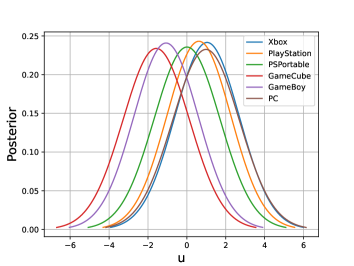
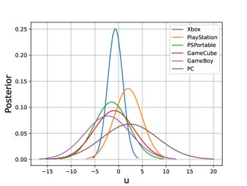
Figure 20: Predictive posterior for the utilities of the platforms. Covariates ownPC=1, age=18 and hours=2 (left), and for covariates ownPlayStation=1, ownPC=1 (right).

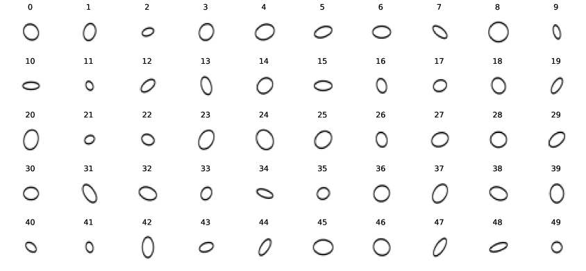
Figure 21: Thumbnail images of the 50 ellipses.

Figure 22: Ellipses shown to the student (ID=32, 15, 25 from left to right). The student selected 15.

6.3 Choosing ellipses

We implemented a gallery demonstration on a computer, showcasing three distinct images of ellipses to a student. These images were randomly selected from the 50 images shown in Figure 21. As it can be seen, these ellipses differ in dimension and orientation relative to the coordinate axes. The task assigned to the student involved selecting ellipses based on two criteria: (i) small eccentricity (being close to a circular shape); (ii) alignment of their axes with the Cartesian axes. It was emphasised to the student that, in case of incomparability due to conflicting criteria, multiple choices were acceptable. Figure 22 shows a screenshot of the image shown to the student and the student’s choice in the caption. Note that, we decreased the resolution of the image to make this task harder. The student repeated this task 160 times generating a dataset including 160 choices, for example $A_{1}=\{6,36,47\},C(A_{1})=\{6\},~{}A_{2}=\{37,42,47\},C(A_{2})=\{37,42\}$.

We use this dataset ($50$ images $25\times 25$ pixels and $160$ choices) to learn the latent utilities through Model 5.2 with pseudo-rational likelihood (since we do not know if the student used Pareto-dominance). The dataset was partitioned into 90% for training and 10% for testing using 10-fold cross-validation, and we computed the accuracy in predicting the student’s choices. More precisely, given a choice set $A$, we computed the most probable choice $\hat{C}(A),\hat{R}(A)$ using the posterior samples of the utility computed according to Model 5.2. Then, given the observed choice $C(A),R(A)$, the accuracy was computed as

$$acc=\frac{1}{|A|}\left(\sum_{o\in C(A)}I_{\hat{C}(A)}(o)+\sum_{v\in R(A)}I_{\hat{R}(A)}(v)\right).$$

The model achieved 84% accuracy. Figure 23(a) depicts the learned utilities for the ellipses presented in Figure 22. As expected, ellipse ID=6 dominates the other ellipses (ID=3 and 23) in both latent utilities. It is worth noting that we do not have explicit labels for the two learned utilities, and their mapping to specific criteria (small eccentricity and alignment to the Cartesian axes) remains unknown. This is analogous to the arbitrary labels in clustering.

Figure 23(b) showcases the utilities for a case of incomparability. Ellipse 15 dominates ID=21 in terms of the first latent utility, whereas ID=21 dominates ID=15 in terms of the second latent utility. The model arrives at a decision that matches the student’s selection, who selected the ellipse $C(A)=\{15,21\}$.

Mostly of the errors result from the ellipses having nearly identical eccentricities and similar aligning to the axes, as shown in Figure 23(c). For $A=\{27,35,41\}$, the model predicts $\hat{C}(A)=\{27,35\}$, while the student selected $\hat{C}(A)=\{35\}$. In these cases, the student’s choices are often wrong. Therefore, the choice model appears to work quite well overall.

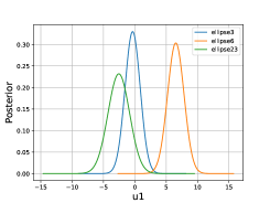
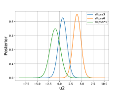
(a)

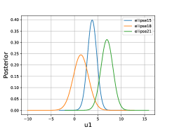
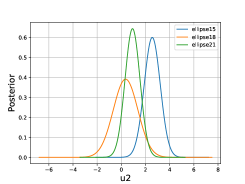
(b)

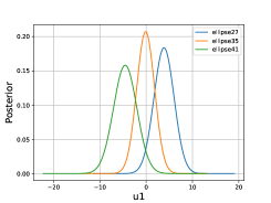
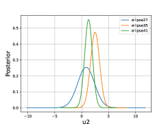
(c)

Figure 23: Predictive posterior for the two latent utilities (top and bottom plot) for the ellipses with (ID=3, 6, 23), (ID=15, 18, 21) and (ID=10, 30, 47).

6.4 Connection with recommender systems

In this section, we will explore the relationship between preference and choice learning within recommendation systems. Additionally, we will discuss how to perform preference and choice learning when dealing with millions of preference pair data.

A recommender system (Aggarwal, 2016) is an algorithm that, given user’s feedback, provides one or more suggestions regarding items that might interest a specific user. Often those systems are based on user-item interactions and use collaborative filtering methods to provide recommendations. In this section we outline how a preference model, such as Model 4.3, can be used as a recommender system.

Let us consider a system with $d$ items $c_{1},\ldots,c_{d}$ and $m$ users ${\bf x}^{(k)}$, $k=1,\ldots,m$. We can assume that we either have explicit interactions (e.g., user’s rankings) or implicit interactions (e.g., browsing history). The recommendation problem consists in providing a suggestion for a new user ${\bf x}^{*}$ or a new (unobserved) suggestion $c_{i}$ to user ${\bf x}^{(k)}$ for some $k$. We can view this task either as the problem of learning the ranking of the $d$ labels for a user ${\bf x}$, or the problem of learning a user’s preferences.

	age	sex	profession
1	24	M	technician
2	53	F	other
3	23	M	writer
4	24	M	technician
5	33	F	other
$\cdots$	$\cdots$	$\cdots$	$\cdots$

	age	sex	technician	other	writer	movie
1	-0.65	1.	1.	0.	0.	0.
2	1.90	0.	0.	1.	0.	0.
$\cdots$	$\cdots$	$\cdots$	$\cdots$	$\cdots$	$\cdots$	$\cdots$
51	-0.65	1.	1.	0.	0.	7.
52	1.90	0.	0.	1.	0.	1.
$\cdots$	$\cdots$	$\cdots$	$\cdots$	$\cdots$	$\cdots$	$\cdots$

movie 1	movie 2
0	350
1	51
$\cdots$	$\cdots$

(a)                                                                                              (b)                                                                                              (c)

Table 5: MovieLens example: (a) users’ features; (b) tiled users’ features with additional feature for pairwise preferences; (c) preference encoding: movie 1 $\succ$ movie 2.

We can frame this task as a preference learning task by rearranging the data in the following format. We assume that, for each user $k$, we have a vector of features ${\bf x}^{(k)}$ that identifies them. Moreover, we can create a sequence of pairwise preferences $c_{i}\succ_{{\bf x}^{(k)}}c_{j}$ for $i,j\in I_{(k)}$, where $I_{(k)}$ is the set of indices identifying the items that have an interaction with user $k$. Note that since $c_{i}\succ_{{\bf x}^{(k)}}c_{j}$ is a pairwise preference, this implies that the user must have chosen the item $c_{i}$ over $c_{j}$. This is available in the data either with an explicit interaction with both $c_{i}$ and $c_{j}$, i.e. the user $k$ ranked $c_{i}$ better than $c_{j}$, or with an implicit interaction, i.e. the user $k$ viewed item $c_{i}$ but not item $c_{j}$. We can further stack all preferences for all available users. Table 5 shows an example of how the data is formatted. We start from the users’ features in Table 5 (a) and with the data “user 1 prefers movie 0 over movie 7” (not shown). We first transform the user features with normalisation and one-hot encoding, first 5 columns of Table 5 (b); then we stack all user features for all movies, as shown in Table 5 (b). Note that Table 5 (b) repeats the features of user 1, in blue, for as many rows as the number of movies. The last column in Table 5 (b) allows us to encode the block diagonal structure of Model 4.3. Finally Table 5 (c) shows the preference encoding: each preference is encoded with a unique movie user pair. For example “user 1 prefers movie 0 over movie 7” is encoded as item 0 $\succ$ item 350 ($7\times 50+0$) and “user 2 prefers movie 0 over movie 1” is encoded as item 0 $\succ$ 51 ($1\times 50+1$). This data structure now allows us to learn the user’s behaviour by using Model 4.3.

We show the effectiveness of this learning procedure on the MovieLens dataset (Harper and Konstan, 2015). The original datasets consists of 100,000 ratings given by $943$ users to $1682$ movies. Each user has rated at least $20$ movies and demographic information is available for each user. We consider a subset of $650$ movies and $50$ users and we generate $2.68$ million pairwise preferences with the procedure outlined above.

Model 4.3 is implemented in GPyTorch (Gardner et al., 2018) and trained with a variational sparse inducing point approximation, $800$ inducing points and stochasic gradient descent on mini-batches of size $5096$. Note that the mini-batch size here is the number of pairwise preferences considered at each gradient step. We compare the performances of this method against Bayesian Personalized Ranking (BPR, Rendle et al. (2009)), a standard Bayesian learning procedure for recommender systems, based on a k-nearest neighbours algorithm. We evaluate the performance with classification metrics: for each new item in the test set an item is correctly classified if the suggested item was preferred by the user. Model 4.3 achieves an accuracy of $0.90$ and a ROC AUC of $0.97$ on the test set. BPR instead achieves an accuracy of $0.71$ and ROC AUC of $0.80$ when trained on the same subset of movies. Note that BPR can be regarded as a linear parametric equivalent of our preference based model. Moreover, our GP-based approach allows us to use the users’ features as covariates to improve the performance, while BPR uses latent features.

7 Conclusions

In this tutorial, we provided an overview of object and label-preference learning using Gaussian Processes. We delved into nine models in detail, exploring their approaches to modelling rational preferences and addressing challenges to deal with irrational preferences such as noisy utilities, comparisons among alternatives with similar utilities, and the presence of conflicting utilities. Lastly, we examined the “duality” between preferences and choices, and introduced a model designed to learn directly from choice data. We showed the application of these models to different datasets and also provided a connection with recommender systems.

We quickly mention here an important application of GP based models: Bayesian optimisation. Preferential Bayesian optimisation has been applied to preference data, as shown in several recent papers (see, e.g., González et al. (2017), Benavoli et al. (2021c), Benavoli et al. (2023b); Takeno et al. (2023)), however research on Bayesian optimisation methods is still very active and work is still required to tailor standard acquisition function to this setting.

The models shown in this tutorial show how to apply Gaussian process models to many preference learning settings. An interesting research direction to be explored is how to learn from a mix of preference data and other type of data sources. For example, a mixed likelihood was proposed in Benavoli et al. (2021a) for data coming from evaluations of the utility function and erroneous preferences. Often an objective evaluation of the utility function is not available, however the users’ response times (see, e.g., Ratcliff and McKoon, 2008) could be recorded. Another direction to improve preference based approaches could be to include this data into the learning process. In certain applications, it is desirable to enforce additional consistency properties on preference and choice data, such as monotonicity and convexity. These properties have been extensively investigated in economics, decision theory and probability theory (Kreps et al., 1990; De Bock and De Cooman, 2019; Seidenfeld et al., 2010; Van Camp et al., 2018). Future research directions include the extension of the models presented in this tutorial to include these other sources of information.

A Proof of Proposition 11 and remarks

Consider the noisy utility model:

$$\widetilde{u}_{i}=u_{i}+v_{i},$$ (68)

fro $i=1,\dots,d$, where we have removed the dependence on the covariates to simplify the notation. Assume that $v_{i}$ is Gumbel distributed with location $0$ and scale $1$, that is its cumulative distribution is $F(v_{i})=e^{-e^{-v_{i}}}$ and its probabiltiy density function is $p(v_{i})=e^{-v_{i}-e^{-v_{i}}}$. Consider the quantity

$$s=\arg\max_{i=1,\dots,d}u_{i}+v_{i},~{}~{}~{}v_{i}\sim\text{Gumbel}(0,1),$$

then we have that

$$P(S=s) =P(\tilde{u}_{s}>\tilde{u}_{i}~{}\forall i\neq s)=\int_{-\infty}^{\infty}P(\tilde{u}_{s}>\tilde{u}_{i}~{}\forall i\neq s|\tilde{u}_{s})p(\tilde{u}_{s})d\tilde{u}_{s}$$

$$=\int_{-\infty}^{\infty}\prod_{i\neq s}P(\tilde{u}_{s}>\tilde{u}_{i}|\tilde{u}_{s})p(\tilde{u}_{s})d\tilde{u}_{s}=\int_{-\infty}^{\infty}\prod_{i\neq s}e^{-e^{u_{i}-\tilde{u}_{s}}}p(\tilde{u}_{s})d\tilde{u}_{s}$$

$$=\int_{-\infty}^{\infty}e^{-\sum_{i\neq s}e^{u_{i}-\tilde{u_{s}}}}e^{u_{s}-\tilde{u_{s}}-e^{u_{s}-\tilde{u_{s}}}}d\tilde{u_{s}}=\int_{-\infty}^{\infty}e^{-\sum_{i}e^{u_{i}-\tilde{u_{s}}}}e^{u_{s}-\tilde{u_{s}}}d\tilde{u_{s}}$$

$$=\int_{-\infty}^{\infty}e^{-e^{-\tilde{u_{s}}}\sum_{i}e^{u_{i}}}e^{u_{s}}e^{-\tilde{u_{s}}}d\tilde{u_{s}}$$

Now if we define $c=\sum_{i}e^{u_{i}}$ then we have that

$$P(S=s) =e^{u_{s}}\int_{-\infty}^{\infty}e^{-ce^{-\tilde{u_{s}}}}e^{-\tilde{u_{s}}}d\tilde{u_{s}}=e^{u_{s}}\int_{-\infty}^{\infty}e^{-\tilde{u_{s}}-ce^{-\tilde{u_{s}}}}d\tilde{u_{s}}=\frac{e^{u_{s}}}{c}=\frac{e^{u_{s}}}{\sum_{i}e^{u_{i}}}.$$

This proves that

$$p(\widetilde{u}_{s}=\max(\widetilde{u}_{1},\dots,\widetilde{u}_{d}))=\frac{a_{s}}{\sum_{j=1}^{d}a_{j}},$$ (69)

with $a_{i}=e^{u_{i}}$.

It is worth noticing that, under normal distributed $v_{i}$, an analogous formula does not hold and also Luce’s axiom of Choice is not satisfied.

B Skew Gaussian Process

The unified skew-normal distribution (Arellano and Azzalini, 2006; Azzalini, 2013; Durante, 2019; Alodat and Shakhatreh, 2020; Anceschi et al., 2023) generalises the normal distribution by introducing skewness. A skew-normal distrbution can be built from a the marginal of a truncated multivariate normal, see (Azzalini, 2013, Ch.7). Consider two vectors ${\bf z}_{0}\in\mathbb{R}^{s},{\bf z}_{1}\in\mathbb{R}^{p}$ such that:

$$\begin{bmatrix}{\bf z}_{1}\\ {\bf z}_{0}\end{bmatrix}\sim N({\bf 0}_{s+p},M),~{}M=\begin{bmatrix}\Omega&\Delta\\ \Delta^{\top}&\Gamma\end{bmatrix},$$ (70)

where $M$ is a full-rank covariance matrix. We then define $\bm{\zeta}$ to be distributed as $({\bf z}_{1}|{\bf z}_{0}+\bm{\gamma}>{\bf 0}_{s})$, where $\bm{\gamma}\in\mathbb{R}^{s}$ and the inequality ${\bf z}_{0}+\bm{\gamma}>{\bf 0}_{s}$ is intended to be component-wise. Then the vector ${\bf z}=\bm{\xi}+\bm{\zeta}\in\mathbb{R}^{p}$ is distributed as a multivariate unified skew-normal distribution with latent skewness dimension $s$. We denote it as ${\bf z}\sim\text{SUN}_{p,s}(\bm{\xi},\Omega,\Delta,\bm{\gamma},\Gamma)$ and its Probability Density Function (PDF) is given by:

$$p({\bf z}) =\phi_{p}({\bf z}-\bm{\xi};\Omega)\frac{\Phi_{s}\left(\bm{\gamma}+\Delta^{\top}{\Omega}^{-1}({\bf z}-\bm{\xi});\Gamma-\Delta^{\top}{\Omega}^{-1}\Delta\right)}{\Phi_{s}\left(\bm{\gamma};\Gamma\right)},$$ (71)

where $\phi_{p}({\bf z}-\bm{\xi};\Omega)$ denotes the PDF of a multivariate normal distribution with mean $\bm{\xi}\in\mathbb{R}^{p}$ and covariance $\Omega\in\mathbb{R}^{p\times p}$. $\Phi_{s}({\bf a};M)$ represents the Cumulative Distribution Function (CDF) of a $s$-dimensional multivariate normal distribution with zero mean and covariance matrix $M$ evaluated at ${\bf a}\in\mathbb{R}^{s}$. The following parameters $\bm{\gamma}\in\mathbb{R}^{s},\Gamma\in\mathbb{R}^{s\times s},\Delta\in\mathbb{R}^{p\times s}$ control the skewness of the distribution. In particular, the parameter $\Delta$ is called skewness matrix. When $\Delta=0$, eq. (71) reduces to $\phi_{p}({\bf z}-\bm{\xi};\Omega)$, i.e. a skew-normal with zero skewness matrix is a normal distribution. Moreover, we assume that $\Phi_{0}(\cdot)=1$, so that, for $s=0$, eq. (71) becomes a multivariate normal distribution. Figure 24 shows the density of a univariate SUN distribution with latent dimensions $s=1$ and $s=2$.

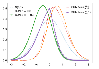
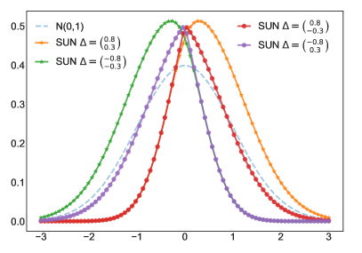
$s=1$, $\Gamma=1$	$s=2$, $\Gamma_{0,1}=\Gamma_{1,0}=0.8$.

Figure 24: Density plots for $\text{SUN}_{1,s}(0,1,\Delta,\gamma,\Gamma)$. For all plots $\Gamma$ is a correlation matrix, $\gamma=0$, dashed blue lines represent the density of $y\sim N_{1}(0,1)$.

A SkewGP (Benavoli et al., 2020, 2021a) is a generalisation of a SUN distribution to a stochastic process which becomes a GP when skewness is zero. To define a SkewGP, we consider a location function $\xi:\mathbb{R}^{d}\rightarrow\mathbb{R}$, a scale (kernel) function $\Omega:\mathbb{R}^{d}\times\mathbb{R}^{d}\rightarrow\mathbb{R}$, a skewness vector function $\Delta:\mathbb{R}^{d}\rightarrow\mathbb{R}^{s}$ and the parameters $\bm{\gamma}\in\mathbb{R}^{s},\Gamma\in\mathbb{R}^{s\times s}$. A real function $f:\mathbb{R}^{d}\rightarrow\mathbb{R}$ is said to be SkewGP-distributed with latent dimension $s$, if for any sequence of $n$ points ${\bf x}_{1},\ldots,{\bf x}_{n}\in\mathbb{R}^{d}$, the vector $[f({\bf x}_{1}),\ldots,f({\bf x}_{n})]^{\top}\in\mathbb{R}^{n}$ is SUN distributed with parameters $\bm{\gamma},\Gamma$ and location, scale and skewness matrices, respectively, given by

$$\begin{array}[]{rl}\xi(X)&=\left[\begin{smallmatrix}\xi({\bf x}_{1}),\xi({\bf x}_{2}),\dots,\xi({\bf x}_{n})\end{smallmatrix}\right]^{\top},\vspace{0.1cm}\\ \Omega(X,X)&=\left[\begin{smallmatrix}\Omega({\bf x}_{1},{\bf x}_{1})&\Omega({\bf x}_{1},{\bf x}_{2})&\dots&\Omega({\bf x}_{1},{\bf x}_{n})\\ \Omega({\bf x}_{2},{\bf x}_{1})&\Omega({\bf x}_{2},{\bf x}_{2})&\dots&\Omega({\bf x}_{2},{\bf x}_{n})\\ \vdots&\vdots&\dots&\vdots\\ \Omega({\bf x}_{n},{\bf x}_{1})&\Omega({\bf x}_{n},{\bf x}_{2})&\dots&\Omega({\bf x}_{n},{\bf x}_{n})\\ \end{smallmatrix}\right],\vspace{0.1cm}\\ \Delta(X)&=\left[\begin{smallmatrix}\Delta({\bf x}_{1}),\Delta({\bf x}_{2}),\dots,\Delta({\bf x}_{n})\\ \end{smallmatrix}\right],\end{array}$$ (72)

where $X=[{\bf x}_{1},{\bf x}_{2},\dots,{\bf x}_{n}]^{\top}$. In this case, we write $f({\bf x})\sim\text{SkewGP}_{s}(\xi({\bf x}),\Omega({\bf x},{\bf x}),\Delta({\bf x}),\bm{\gamma},\Gamma)$. SkewGPs are conjugate with both the normal and affine probit likelihood and, more in general, with their product. This allows us to derive their posterior for nonparametric regression, classification, preference learning and mixed problems.

In particular, consider the affine-probit-normal product likelihood:

$$p(Y,Z,W\mid f(X)) =\Phi_{m_{a}}(Z+Wf(X);\Sigma)\phi_{m_{r}}(Y-Cf(X);R).$$ (73)

where $m_{r}$ (the subscript $r$ stands for regression) denotes the number of regression-type observations and $m_{a}$ the number of binary/preference-type observations (the subscript $a$ stands for affine). Therefore, we have that $Y\in\mathbb{R}^{m_{r}},C\in\mathbb{R}^{m_{r}\times n},W\in\mathbb{R}^{m_{a}\times n},Z\in\mathbb{R}^{m_{a}\times 1}$. The matrices $\Sigma\in\mathbb{R}^{m_{a}\times m_{a}},R\in\mathbb{R}^{m_{r}\times m_{r}}$ are covariance matrices. This likelihood encompasses all the standard likelihood functions used in regression, classification and preference-learning. For instance, a standard regression is obtained by setting $C=I_{m_{r}}$, $R=\sigma^{2}I_{m_{r}}$ and $m_{a}=0$; classification is obtained for $W=diag(2Y-1)$, $Z={\bf 0}_{m_{a}}$, $\Sigma=I_{m_{a}}$ and $m_{r}=0$, where $Y$ is the vector containing the observed class values $Y_{i}\in\{0,1\}$. Preference learning is obtained with $Z={\bf 0}_{m_{a}}$, $\Sigma=I_{m_{a}}$ and $m_{r}=0$ and $W\in\mathbb{R}^{m_{a}\times n}$ whose s-th row is all zero apart from $W_{i}=1,W_{j}=-1$ if the data includes the preference ${\bf x}_{i}\succ{\bf x}_{j}$.

We now include this result from (Benavoli et al., 2021a, Theorem 3).

Proposition 16

Let us assume a SkewGP prior $f({\bf x})\sim\text{SkewGP}_{s}(\xi({\bf x}),\Omega({\bf x},{\bf x}),\Delta({\bf x}),\bm{\gamma},\Gamma)$, the likelihood (73), then a-posteriori $f({\bf x})$ is SkewGP with mean, covariance and skewness functions:

$$\tilde{\bm{\xi}}({\bf x}) =\bm{\xi}({\bf x})+\Omega({\bf x},X)C^{T}(C\Omega(X,X)C^{T}+R)^{-1}(Y-C\xi(X)),$$

$$\tilde{\Omega}({\bf x},{\bf x}) =\Omega({\bf x},{\bf x})-\Omega({\bf x},X)C^{T}(C\Omega(X,X)C^{T}+R)^{-1}C\Omega(X,{\bf x}),$$

$$\tilde{\Delta}({\bf x}) =\begin{bmatrix}\Delta({\bf x})~{}&\Omega({\bf x},X)W^{T}\end{bmatrix}-\Omega({\bf x},X)C^{T}(C\Omega(X,X)C^{T}+R)^{-1}C\begin{bmatrix}\Delta(X)~{}&\Omega(X,X)W^{T}\end{bmatrix},$$

$$\tilde{\bm{\gamma}} =\bm{\gamma}_{p}+\begin{bmatrix}\Delta(X)~{}&\Omega(X,X)W^{T}\end{bmatrix}^{T}{\Omega}(X,X)^{-1}(\tilde{\bm{\xi}}(X)-\bm{\xi}(X))$$

$$\tilde{\Gamma} =\Gamma_{p}-\begin{bmatrix}\Delta(X)~{}&\Omega(X,X)W^{T}\end{bmatrix}^{T}\Omega^{-1}(X,X)\begin{bmatrix}\Delta(X)~{}&\Omega(X,X)W^{T}\end{bmatrix}+\Delta_{p}^{T}\tilde{\Omega}(X,X)^{-1}\Delta_{p},$$

$$\Delta_{p} =\tilde{\Omega}(X,X){\Omega}^{-1}(X,X)\begin{bmatrix}\Delta(X)~{}&\Omega(X,X)W^{T}\end{bmatrix},$$

$$\bm{\gamma}_{p} =[\bm{\gamma},~{}~{}Z+W\xi(X)]^{T},$$

$$\Gamma_{p} =\begin{bmatrix}\Gamma&~{}~{}\Delta(X)^{T}W^{T}\\ W\Delta(X)&~{}~{}(W\Omega(X,X)W^{T}+\Sigma)\end{bmatrix}.$$

The computation of predictive inference (posterior mean, credible intervals etc.) can be achieved by sampling. Note that (Azzalini, 2013, Ch.7) that
$\mathbf{z}\sim\operatorname{SUN}_{p,s}(\bm{\xi},\Omega,\Delta,\bm{\gamma},\Gamma)$ can be written as $\mathbf{z}=\bm{\xi}+\mathbf{r}_{0}+\Delta\Gamma^{-1}\mathbf{r}_{1,-\gamma}$ with $\mathbf{r}_{0}\sim\phi_{p}(0;\bar{\Omega}-\Delta\Gamma^{-1}\Delta^{T})$ and $\mathbf{r}_{1,-\gamma}$ is the truncation below $\gamma$ of $\mathbf{r}_{1}\sim\phi_{s}(0;\Gamma)$. Samples of the vector $\mathbf{r}_{0}$ can be achieved efficiently with standard methods, and $\mathbf{r}_{1,-\gamma}$ can be obtained efficiently using the methods discussed in Section 3.1. Similarly to GPs, the functions and matrices defining a SkewGP, $\text{SkewGP}_{s}(\xi({\bf x}),\Omega({\bf x},{\bf x}),\Delta({\bf x}),\bm{\gamma},\Gamma)$ may depend on hyperparamters ${\bm{\theta}}$. These parameters are usually estimated by maximising the marginal likelihood, which is equal to:

$$p(Y)=\phi_{m_{r}}(Y-C\xi(X);C\Omega(X,X)C^{T}+R)\frac{\Phi_{s+m_{a}}(\tilde{\bm{\gamma}};~{}\tilde{\Gamma})}{\Phi_{s}(\bm{\gamma};~{}\Gamma)},$$ (74)

with $\tilde{\bm{\gamma}},\tilde{\Gamma}$ are defined in Proposition 16. This involves the computation of a high-dimensional multivariate CDFs $\Phi_{s+m_{a}}(\cdot),\Phi_{s}(\cdot)$. In this tutorial, we use the Laplace’s approximation to approximate this integral.

C PrefGP library

This tutorial is supported by a Python software library, prefGP (Benavoli and Azzimonti, 2024), that implements Models 1-9 and reproduces the results presented in the paper via notebooks. Further models can be developed by modifying the likelihood, as the inference process relies on generic Laplace’s and Variational approximations (implemented using either Jax or PyTorch).

References

- Adam and Destercke (2021a) Loïc Adam and Sébastien Destercke. Incremental elicitation of preferences: optimist or pessimist? In Algorithmic Decision Theory: 7th International Conference, ADT 2021, Toulouse, France, November 3–5, 2021, Proceedings 7, pages 71–85. Springer, 2021a.
- Adam and Destercke (2021b) Loïc Adam and Sébastien Destercke. Possibilistic preference elicitation by minimax regret. In Uncertainty in artificial intelligence, pages 718–727. PMLR, 2021b.
- Agarwal et al. (2018) Arpit Agarwal, Prathamesh Patil, and Shivani Agarwal. Accelerated spectral ranking. In International Conference on Machine Learning, pages 70–79. PMLR, 2018.
- Aggarwal (2016) Charu C. Aggarwal. Recommender Systems. Springer International Publishing, Cham, 2016. ISBN 978-3-319-29657-9. doi: 10.1007/978-3-319-29659-3.
- Aiolli and Sperduti (2004) Fabio Aiolli and Alessandro Sperduti. Learning preferences for multiclass problems. Advances in neural information processing systems, 17, 2004.
- Aizerman and Malishevski (1981) Mark Aizerman and Andrew Malishevski. General theory of best variants choice: Some aspects. IEEE Transactions on Automatic Control, 26(5):1030–1040, 1981.
- Alodat and Shakhatreh (2020) MT Alodat and Mohammed K Shakhatreh. Gaussian process regression with skewed errors. Journal of Computational and Applied Mathematics, 370:112665, 2020.
- Alvo and Philip (2014) Mayer Alvo and LH Philip. Statistical methods for ranking data, volume 1341. Springer, 2014.
- Anceschi et al. (2023) Niccolò Anceschi, Augusto Fasano, Daniele Durante, and Giacomo Zanella. Bayesian conjugacy in probit, tobit, multinomial probit and extensions: A review and new results. Journal of the American Statistical Association, 118(542):1451–1469, 2023.
- Arellano and Azzalini (2006) R. B Arellano and Adelchi Azzalini. On the unification of families of skew-normal distributions. Scandinavian Journal of Statistics, 33(3):561–574, 2006.
- Arlegi and Teschl (2022) Ricardo Arlegi and Miriam Teschl. Pareto rationalizability by two single-peaked preferences. Mathematical Social Sciences, 118:1–11, 2022.
- Arrow (1963) Kenneth J Arrow. Social choice and individual values. Yale university press, 1963.
- Azari et al. (2012) Hossein Azari, David Parks, and Lirong Xia. Random utility theory for social choice. Advances in Neural Information Processing Systems, 25, 2012.
- Azari Soufiani et al. (2013) Hossein Azari Soufiani, William Chen, David C Parkes, and Lirong Xia. Generalized method-of-moments for rank aggregation. Advances in Neural Information Processing Systems, 26, 2013.
- Azzalini (2013) Adelchi Azzalini. The skew-normal and related families, volume 3. Cambridge University Press, 2013.
- Bauer et al. (2016) Matthias Bauer, Mark van der Wilk, and Carl Edward Rasmussen. Understanding probabilistic sparse Gaussian process approximations. In Advances in neural information processing systems, pages 1533–1541, 2016.
- Benavoli and Azzimonti (2024) Alessio Benavoli and Dario Azzimonti. prefGP: A python package for preference and choice learning with gaussian processes. https://github.com/benavoli/prefGP, 2024.
- Benavoli et al. (2020) Alessio Benavoli, Dario Azzimonti, and Dario Piga. Skew Gaussian Processes for Classification. Machine Learning, 109:1877–1902, 2020. doi: 10.1007/s10994-020-05906-3. URL https://arxiv.org/abs/2005.12987.
- Benavoli et al. (2021a) Alessio Benavoli, Dario Azzimonti, and Dario Piga. A unified framework for closed-form nonparametric regression, classification, preference and mixed problems with Skew Gaussian Processes. Machine Learning, pages 1–39, 2021a. doi: 10.1007/s10994-021-06039-x. URL https://link.springer.com/article/10.1007/s10994-021-06039-x.
- Benavoli et al. (2021b) Alessio Benavoli, Dario Azzimonti, and Dario Piga. Preferential Bayesian optimisation with Skew Gaussian Processes. In 2021 Genetic and Evolutionary Computation Conference Companion (GECCO ’21 Companion), July 10–14, 2021, Lille, France, New York, NY, USA, 2021b. ACM.
- Benavoli et al. (2021c) Alessio Benavoli, Dario Azzimonti, and Dario Piga. Preferential bayesian optimisation with skew gaussian processes. In Proceedings of the Genetic and Evolutionary Computation Conference Companion, pages 1842–1850, 2021c.
- Benavoli et al. (2023a) Alessio Benavoli, Dario Azzimonti, and Dario Piga. Learning choice functions with gaussian processes. In Robin J. Evans and Ilya Shpitser, editors, Proceedings of the Thirty-Ninth Conference on Uncertainty in Artificial Intelligence, volume 216 of Proceedings of Machine Learning Research, pages 141–151. PMLR, 2023a. URL https://proceedings.mlr.press/v216/benavoli23a.html.
- Benavoli et al. (2023b) Alessio Benavoli, Dario Azzimonti, and Dario Piga. Bayesian optimization for choice data. In 2023 Genetic and Evolutionary Computation Conference Companion (GECCO ’23 Companion), July 15–19, 2023, Lisbon, 2023b. doi: 10.1145/3583133.3596324.
- Benson et al. (2018) Austin R Benson, Ravi Kumar, and Andrew Tomkins. A discrete choice model for subset selection. In Proceedings of the eleventh ACM international conference on web search and data mining, pages 37–45, 2018.
- Bierlaire (2018) Michel Bierlaire. Pandasbiogeme: a short introduction. Report TRANSP-OR: Lausanne, Switzerland, 181219, 2018.
- Botev (2017) Zdravko I Botev. The normal law under linear restrictions: simulation and estimation via minimax tilting. Journal of the Royal Statistical Society Series B: Statistical Methodology, 79(1):125–148, 2017.
- Bourdache et al. (2019) Nadjet Bourdache, Patrice Perny, and Olivier Spanjaard. Incremental elicitation of rank-dependent aggregation functions based on bayesian linear regression. In IJCAI-19-Twenty-Eighth International Joint Conference on Artificial Intelligence, pages 2023–2029. International Joint Conferences on Artificial Intelligence Organization, 2019.
- Boutilier (2013) Craig Boutilier. Computational decision support: Regret-based models for optimization and preference elicitation, 2013.
- Boutilier et al. (2006) Craig Boutilier, Relu Patrascu, Pascal Poupart, and Dale Schuurmans. Constraint-based optimization and utility elicitation using the minimax decision criterion. Artificial Intelligence, 170(8-9):686–713, 2006.
- Bradley and Terry (1952) Ralph Allan Bradley and Milton E Terry. Rank analysis of incomplete block designs: I. the method of paired comparisons. Biometrika, 39(3/4):324–345, 1952.
- Brathwaite and Walker (2018) Timothy Brathwaite and Joan L Walker. Asymmetric, closed-form, finite-parameter models of multinomial choice. Journal of choice modelling, 29:78–112, 2018.
- Burges et al. (2005) Chris Burges, Tal Shaked, Erin Renshaw, Ari Lazier, Matt Deeds, Nicole Hamilton, and Greg Hullender. Learning to rank using gradient descent. In Proceedings of the 22nd international conference on Machine learning, pages 89–96, 2005.
- Burges (2010) Christopher JC Burges. From ranknet to lambdarank to lambdamart: An overview. Learning, 11(23-581):81, 2010.
- Caragiannis et al. (2016) Ioannis Caragiannis, Ariel D. Procaccia, and Nisarg Shah. When do noisy votes reveal the truth? ACM Transactions on Economics and Computation, 4(3):1–30, Jun 2016. ISSN 2167-8375, 2167-8383. doi: 10.1145/2892565.
- Caron and Doucet (2012) Francois Caron and Arnaud Doucet. Efficient bayesian inference for generalized bradley–terry models. Journal of Computational and Graphical Statistics, 21(1):174–196, 2012.
- Chernoff (1954) Herman Chernoff. Rational selection of decision functions. Econometrica: journal of the Econometric Society, pages 422–443, 1954.
- Christiano et al. (2017) Paul F Christiano, Jan Leike, Tom Brown, Miljan Martic, Shane Legg, and Dario Amodei. Deep reinforcement learning from human preferences. Advances in neural information processing systems, 30, 2017.
- Chu and Ghahramani (2005) Wei Chu and Zoubin Ghahramani. Preference Learning with Gaussian Processes. In Proceedings of the 22nd International Conference on Machine Learning, ICML ’05, page 137–144, New York, NY, USA, 2005. Association for Computing Machinery. ISBN 1595931805. doi: 10.1145/1102351.1102369.
- Cohen et al. (1997) William W Cohen, Robert E Schapire, and Yoram Singer. Learning to order things. Advances in neural information processing systems, 10, 1997.
- Critchlow and Fligner (1991) Douglas E Critchlow and Michael A Fligner. Paired comparison, triple comparison, and ranking experiments as generalized linear models, and their implementation on glim. Psychometrika, 56(3):517–533, 1991.
- Croissant (2020) Yves Croissant. Estimation of random utility models in r: the mlogit package. Journal of Statistical Software, 95:1–41, 2020.
- De Bock and De Cooman (2019) Jasper De Bock and Gert De Cooman. Interpreting, axiomatising and representing coherent choice functions in terms of desirability. In International Symposium on Imprecise Probabilities: Theories and Applications, pages 125–134. PMLR, 2019.
- Debreu (1954) Gerard Debreu. Representation of a preference ordering by a numerical function. Decision processes, 3:159–165, 1954.
- Du et al. (2023) Tianyu Du, Ayush Kanodia, and Susan Athey. Torch-choice: A pytorch package for large-scale choice modelling with python. arXiv preprint arXiv:2304.01906, 2023.
- Durante (2019) Daniele Durante. Conjugate Bayes for probit regression via unified skew-normal distributions. Biometrika, 106(4):765–779, 08 2019.
- Eliaz and Ok (2006) Kfir Eliaz and Efe A Ok. Indifference or indecisiveness? choice-theoretic foundations of incomplete preferences. Games and economic behavior, 56(1):61–86, 2006.
- Eric et al. (2007) Brochu Eric, Nando Freitas, and Abhijeet Ghosh. Active preference learning with discrete choice data. Advances in neural information processing systems, 20, 2007.
- Evgeniou et al. (2005) Theodoros Evgeniou, Constantinos Boussios, and Giorgos Zacharia. Generalized robust conjoint estimation. Marketing Science, 24(3):415–429, 2005.
- Fiechter and Rogers (2000) Claude-Nicolas Fiechter and Seth Rogers. Learning subjective functions with large margins. In ICML, pages 287–294, 2000.
- Fishburn (1988) Peter C. Fishburn. Nonlinear preference and utility theory. Johns Hopkins series in the mathematical sciences. Johns Hopkins University Press, Baltimore, 1988. ISBN 978-0-8018-3598-8.
- Fligner and Verducci (1990) Michael A Fligner and Joseph S Verducci. Posterior probabilities for a consensus ordering. Psychometrika, 55:53–63, 1990.
- Fok et al. (2012) Dennis Fok, Richard Paap, and Bram Van Dijk. A rank-ordered logit model with unobserved heterogeneity in ranking capabilities. Journal of applied econometrics, 27(5):831–846, 2012.
- Forinash and Koppelman (1993) Christopher V Forinash and Frank S Koppelman. Application and interpretation of nested logit models of intercity mode choice. Transportation research record, (1413), 1993.
- Fürnkranz and Hüllermeier (2010) Johannes Fürnkranz and Eyke Hüllermeier. Preference learning. Springer, 2010.
- Gardner et al. (2018) Jacob R. Gardner, Geoff Pleiss, David Bindel, Kilian Q. Weinberger, and Andrew Gordon Wilson. Gpytorch: Blackbox matrix-matrix gaussian process inference with gpu acceleration. Advances in Neural Information Processing Systems, 2018-Decem(NeurIPS):7576–7586, 2018. ISSN 10495258. arXiv: 1809.11165.
- Gessner et al. (2020) Alexandra Gessner, Oindrila Kanjilal, and Philipp Hennig. Integrals over Gaussians under Linear Domain Constraints. In Silvia Chiappa and Roberto Calandra, editors, Proceedings of the Twenty Third International Conference on Artificial Intelligence and Statistics, volume 108, pages 2764–2774. PMLR, 26–28 Aug 2020.
- Gibbs and MacKay (2000) Mark N Gibbs and David JC MacKay. Variational Gaussian process classifiers. IEEE Transactions on Neural Networks, 11(6):1458–1464, 2000.
- González et al. (2017) Javier González, Zhenwen Dai, Andreas Damianou, and Neil D. Lawrence. Preferential Bayesian Optimization. In Proceedings of the 34th International Conference on Machine Learning, pages 1282–1291. PMLR, 2017. URL https://proceedings.mlr.press/v70/gonzalez17a.html.
- Guiver and Snelson (2009) John Guiver and Edward Snelson. Bayesian inference for plackett-luce ranking models. In proceedings of the 26th annual international conference on machine learning, pages 377–384, 2009.
- Har-Peled et al. (2002) Sariel Har-Peled, Dan Roth, and Dav Zimak. Constraint classification: A new approach to multiclass classification. In International conference on algorithmic learning theory, pages 365–379. Springer, 2002.
- Harper and Konstan (2015) F. Maxwell Harper and Joseph A. Konstan. The MovieLens Datasets: History and Context. ACM Transactions on Interactive Intelligent Systems, 5(4):19:1–19:19, 2015. ISSN 2160-6455. doi: 10.1145/2827872.
- Hensman et al. (2013) James Hensman, Nicolò Fusi, and Neil D. Lawrence. Gaussian processes for big data. In Proceedings of the Twenty-Ninth Conference on Uncertainty in Artificial Intelligence, UAI’13, pages 282–290, Arlington, Virginia, USA, 2013. AUAI Press.
- Herbrich et al. (1998) Ralf Herbrich, Thore Graepel, Peter Bollmann-Sdorra, and Klaus Obermayer. Learning preference relations for information retrieval. In ICML-98 Workshop: text categorization and machine learning, pages 80–84, 1998.
- Hernandez-Lobato and Hernandez-Lobato (2016) Daniel Hernandez-Lobato and Jose Miguel Hernandez-Lobato. Scalable gaussian process classification via expectation propagation. In Proceedings of the 19th International Conference on Artificial Intelligence and Statistics, page 168–176. PMLR, 2016. URL https://proceedings.mlr.press/v51/hernandez-lobato16.html.
- Hess and Palma (2019) Stephane Hess and David Palma. Apollo: A flexible, powerful and customisable freeware package for choice model estimation and application. Journal of choice modelling, 32:100170, 2019.
- Houlsby et al. (2011) Neil Houlsby, Ferenc Huszár, Zoubin Ghahramani, and Máté Lengyel. Bayesian active learning for classification and preference learning. arXiv preprint arXiv:1112.5745, 2011.
- Hüllermeier et al. (2008) Eyke Hüllermeier, Johannes Fürnkranz, Weiwei Cheng, and Klaus Brinker. Label ranking by learning pairwise preferences. Artificial Intelligence, 172(16-17):1897–1916, 2008.
- Hunter (2004) David R Hunter. MM algorithms for generalized Bradley-Terry models. The Annals of Statistics, 32(1):384–406, 2004.
- Kotecha and Djuric (1999) Jayesh H Kotecha and Petar M Djuric. Gibbs sampling approach for generation of truncated multivariate gaussian random variables. In 1999 IEEE International Conference on Acoustics, Speech, and Signal Processing. Proceedings. ICASSP99 (Cat. No. 99CH36258), volume 3, pages 1757–1760. IEEE, 1999.
- Kreps et al. (1990) David M Kreps et al. A course in microeconomic theory. Princeton university press, 1990.
- Lederrey et al. (2021) Gael Lederrey, Virginie Lurkin, Tim Hillel, and Michel Bierlaire. Estimation of discrete choice models with hybrid stochastic adaptive batch size algorithms. Journal of Choice Modelling, 38:100226, 2021. ISSN 1755-5345.
- Lomeli et al. (2019) Maria Lomeli, Mark Rowland, Arthur Gretton, and Zoubin Ghahramani. Antithetic and monte carlo kernel estimators for partial rankings. Statistics and Computing, 29:1127–1147, 2019.
- Luce (1956) R Duncan Luce. Semiorders and a theory of utility discrimination. Econometrica, Journal of the Econometric Society, pages 178–191, 1956.
- Luce (1959) R Duncan Luce. Individual Choice Behavior: A Theoretical Analysis. Wiley, New York, 1959.
- Lun Chau et al. (2022) Siu Lun Chau, Javier Gonzalez, and Dino Sejdinovic. Learning Inconsistent Preferences with Gaussian Processes. In Gustau Camps-Valls, Francisco J. R. Ruiz, and Isabel Valera, editors, Proceedings of The 25th International Conference on Artificial Intelligence and Statistics, volume 151 of Proceedings of Machine Learning Research, pages 2266–2281. PMLR, 2022. URL https://proceedings.mlr.press/v151/lun-chau22a.html.
- MacKay (1996) David JC MacKay. Bayesian methods for backpropagation networks. In Models of neural networks III, pages 211–254. Springer, 1996.
- Maldonado et al. (2015) Sebastián Maldonado, Ricardo Montoya, and Richard Weber. Advanced conjoint analysis using feature selection via support vector machines. European Journal of Operational Research, 241(2):564–574, 2015.
- Mallows (1957) Colin L Mallows. Non-null ranking models. i. Biometrika, 44(1/2):114–130, 1957.
- Marden (1996) John I Marden. Analyzing and modeling rank data. CRC Press, 1996.
- Maystre and Grossglauser (2015) Lucas Maystre and Matthias Grossglauser. Fast and accurate inference of plackett–luce models. Advances in neural information processing systems, 28, 2015.
- McFadden (1974) Daniel McFadden. The measurement of urban travel demand. Journal of Public Economics, 3(4):303–328, 1974.
- McFadden (1978) Daniel McFadden. Modeling the choice of residential location. In Handbook of Regional and Urban Economics, volume 2, pages 753–803. 1978.
- Meilă et al. (2007) Marina Meilă, Kapil Phadnis, Arthur Patterson, and Jeff Bilmes. Consensus ranking under the exponential model. In Proceedings of the Twenty-Third Conference on Uncertainty in Artificial Intelligence, UAI’07, page 285–294, Arlington, Virginia, USA, 2007. AUAI Press. ISBN 978-0-9749039-3-4. URL http://arxiv.org/abs/1206.5265. arXiv:1206.5265 [cs, stat].
- Minka (2001) Thomas Peter Minka. A family of algorithms for approximate Bayesian inference. PhD thesis, Massachusetts Institute of Technology, 2001.
- Mosteller and Nogee (1951) Frederick Mosteller and Philip Nogee. An experimental measurement of utility. Journal of Political Economy, 59(5):371–404, 1951.
- Moulin (1985) Hervé Moulin. Choice functions over a finite set: a summary. Social Choice and Welfare, 2(2):147–160, 1985.
- Negahban et al. (2012) Sahand Negahban, Sewoong Oh, and Devavrat Shah. Iterative ranking from pair-wise comparisons. Advances in neural information processing systems, 25, 2012.
- Nguyen et al. (2021) Quoc Phong Nguyen, Sebastian Tay, Bryan Kian Hsiang Low, and Patrick Jaillet. Top-k ranking bayesian optimization. Proceedings of the AAAI Conference on Artificial Intelligence, 35(1010):9135–9143, 2021. ISSN 2374-3468. doi: 10.1609/aaai.v35i10.17103.
- O’Hagan (1978) Anthony O’Hagan. Curve fitting and optimal design for prediction. Journal of the Royal Statistical Society: Series B (Methodological), 40(1):1–24, 1978.
- Opper and Archambeau (2009) Manfred Opper and Cédric Archambeau. The variational gaussian approximation revisited. Neural computation, 21(3):786–792, 2009.
- Ouyang et al. (2022) Long Ouyang, Jeffrey Wu, Xu Jiang, Diogo Almeida, Carroll Wainwright, Pamela Mishkin, Chong Zhang, Sandhini Agarwal, Katarina Slama, Alex Ray, et al. Training language models to follow instructions with human feedback. Advances in Neural Information Processing Systems, 35:27730–27744, 2022.
- Pahikkala et al. (2010) Tapio Pahikkala, Willem Waegeman, Evgeni Tsivtsivadze, Tapio Salakoski, and Bernard De Baets. Learning intransitive reciprocal relations with kernel methods. European Journal of Operational Research, 206(3):676–685, 2010.
- Pakman and Paninski (2014) Ari Pakman and Liam Paninski. Exact hamiltonian monte carlo for truncated multivariate gaussians. Journal of Computational and Graphical Statistics, 23(2):518–542, 2014.
- Pfannschmidt and Hüllermeier (2020) Karlson Pfannschmidt and Eyke Hüllermeier. Learning Choice Functions via Pareto-Embeddings. In German Conference on Artificial Intelligence (Künstliche Intelligenz), pages 327–333. Springer, 2020.
- Pfannschmidt et al. (2022) Karlson Pfannschmidt, Pritha Gupta, Björn Haddenhorst, and Eyke Hüllermeier. Learning context-dependent choice functions. International Journal of Approximate Reasoning, 140:116–155, 2022.
- Plackett (1975) Robin L Plackett. The analysis of permutations. Journal of the Royal Statistical Society Series C: Applied Statistics, 24(2):193–202, 1975.
- Quiñonero-Candela and Rasmussen (2005) Joaquin Quiñonero-Candela and Carl Edward Rasmussen. A unifying view of sparse approximate Gaussian process regression. Journal of Machine Learning Research, 6(Dec):1939–1959, 2005.
- Rafailov et al. (2023) Rafael Rafailov, Archit Sharma, Eric Mitchell, Christopher D Manning, Stefano Ermon, and Chelsea Finn. Direct preference optimization: Your language model is secretly a reward model. In A. Oh, T. Neumann, A. Globerson, K. Saenko, M. Hardt, and S. Levine, editors, Advances in Neural Information Processing Systems, volume 36, page 53728–53741. Curran Associates, Inc., 2023. URL https://proceedings.neurips.cc/paper_files/paper/2023/file/a85b405ed65c6477a4fe8302b5e06ce7-Paper-Conference.pdf.
- Ragain and Ugander (2016) Stephen Ragain and Johan Ugander. Pairwise choice markov chains. Advances in neural information processing systems, 29, 2016.
- Rasmussen and Williams (2006) Carl Edward Rasmussen and Christopher KI Williams. Gaussian processes for machine learning. MIT press Cambridge, MA, 2006.
- Ratcliff and McKoon (2008) Roger Ratcliff and Gail McKoon. The diffusion decision model: Theory and data for two-choice decision tasks. Neural computation, 20(4):873–922, 2008. ISSN 0899-7667. doi: 10.1162/neco.2008.12-06-420.
- Rendle et al. (2009) Steffen Rendle, Christoph Freudenthaler, Zeno Gantner, and Lars Schmidt-Thieme. Bpr: Bayesian personalized ranking from implicit feedback. In Proceedings of the Twenty-Fifth Conference on Uncertainty in Artificial Intelligence, UAI ’09, pages 452–461, Arlington, Virginia, USA, 2009. AUAI Press. ISBN 978-0-9749039-5-8.
- Ricci et al. (2015) Francesco Ricci, Lior Rokach, and Bracha Shapira. Recommender systems: introduction and challenges. Recommender systems handbook, pages 1–34, 2015.
- Samuelson (1938) Paul A Samuelson. A note on the pure theory of consumer’s behaviour. Economica, 5(17):61–71, 1938.
- Schuerch et al. (2020) Manuel Schuerch, Dario Azzimonti, Alessio Benavoli, and Marco Zaffalon. Recursive estimation for sparse Gaussian process regression. Automatica, 120:109–127, 2020. ISSN 0005-1098.
- Schuerch et al. (2023) Manuel Schuerch, Dario Azzimonti, Alessio Benavoli, and Marco Zaffalon. Correlated product of experts for sparse gaussian process regression. Machine Learning, 2023. doi: 10.1007/s10994-022-06297-3.
- Schwartz (1986) Thomas Schwartz. Chapter 1. Choice Functions, pages 11–23. Columbia University Press, New York Chichester, West Sussex, 1986. ISBN 9780231895309. doi: doi:10.7312/schw93758-004. URL https://doi.org/10.7312/schw93758-004.
- Seidenfeld et al. (2010) Teddy Seidenfeld, Mark J Schervish, and Joseph B Kadane. Coherent choice functions under uncertainty. Synthese, 172(1):157–176, 2010.
- Sen (1971) Amartya K Sen. Choice functions and revealed preference. The Review of Economic Studies, 38(3):307–317, 1971.
- Shafer (1974) Wayne J Shafer. The nontransitive consumer. Econometrica: Journal of the Econometric Society, pages 913–919, 1974.
- Shah et al. (2015) Nihar Shah, Sivaraman Balakrishnan, Joseph Bradley, Abhay Parekh, Kannan Ramchandran, and Martin Wainwright. Estimation from pairwise comparisons: Sharp minimax bounds with topology dependence. In Artificial intelligence and statistics, pages 856–865. PMLR, 2015.
- Shahriari et al. (2015) Bobak Shahriari, Kevin Swersky, Ziyu Wang, Ryan P Adams, and Nando De Freitas. Taking the human out of the loop: A review of Bayesian optimization. Proceedings of the IEEE, 104(1):148–175, 2015.
- Sifringer et al. (2020) Brian Sifringer, Virginie Lurkin, and Alexandre Alahi. Enhancing discrete choice models with representation learning. Transportation Research Part B: Methodological, 140:236–261, 2020. ISSN 0191-2615.
- Siivola et al. (2021) Eero Siivola, Akash Kumar Dhaka, Michael Riis Andersen, Javier González, Pablo García Moreno, and Aki Vehtari. Preferential Batch Bayesian Optimization. In 2021 IEEE 31st International Workshop on Machine Learning for Signal Processing (MLSP), pages 1–6. IEEE, 2021.
- Smith (1950) B Babington Smith. Discussion of professor ross’s paper. Journal of the Royal Statistical Society B, 12(1):41–59, 1950.
- Snelson and Ghahramani (2006) Edward Snelson and Zoubin Ghahramani. Sparse Gaussian processes using pseudo-inputs. In Advances in neural information processing systems, pages 1257–1264, 2006.
- Stiennon et al. (2020) Nisan Stiennon, Long Ouyang, Jeffrey Wu, Daniel Ziegler, Ryan Lowe, Chelsea Voss, Alec Radford, Dario Amodei, and Paul F Christiano. Learning to summarize with human feedback. Advances in Neural Information Processing Systems, 33:3008–3021, 2020.
- Takeno et al. (2023) Shion Takeno, Masahiro Nomura, and Masayuki Karasuyama. Towards practical preferential bayesian optimization with skew gaussian processes. In Proceedings of the 40th International Conference on Machine Learning, page 33516–33533. PMLR, July 2023. URL https://proceedings.mlr.press/v202/takeno23b.html.
- Taylor and Benjamini (2016) J Taylor and Y Benjamini. Restrictedmvn: multivariate normal restricted by affine constraints. R package version, 1, 2016.
- Thurstone (1927) Louis L. Thurstone. A law of comparative judgment. Psychological Review, 34(4):273–286, Jul 1927. ISSN 1939-1471, 0033-295X. doi: 10.1037/h0070288.
- Titsias (2009) Michalis Titsias. Variational learning of inducing variables in sparse Gaussian processes. In David van Dyk and Max Welling, editors, Proceedings of the Twelth International Conference on Artificial Intelligence and Statistics, volume 5 of Proceedings of Machine Learning Research, pages 567–574, Hilton Clearwater Beach Resort, Clearwater Beach, Florida USA, 16–18 Apr 2009. PMLR.
- Train (2009) Kenneth E Train. Discrete choice methods with simulation. Cambridge university press, 2009.
- Troffaes and Goldstein (2013) Matthias Troffaes and Michael Goldstein. A note on the temporal sure preference principle and the updating of lower previsions. In 8th International Symposium on Imprecise Probability: Theories and Applications, Compiegne, France, 2013.
- Tversky and Simonson (1993) Amos Tversky and Itamar Simonson. Context-dependent preferences. Management science, 39(10):1179–1189, 1993.
- Van Camp et al. (2018) Arthur Van Camp, Gert De Cooman, Enrique Miranda, and Erik Quaeghebeur. Coherent choice functions, desirability and indifference. Fuzzy sets and systems, 341:1–36, 2018.
- van Cranenburgh et al. (2022) Sander van Cranenburgh, Shenhao Wang, Akshay Vij, Francisco Pereira, and Joan Walker. Choice modelling in the age of machine learning-discussion paper. Journal of Choice Modelling, 42:100340, 2022.
- Vojnovic and Yun (2016) Milan Vojnovic and Seyoung Yun. Parameter estimation for generalized thurstone choice models. In International Conference on Machine Learning, pages 498–506. PMLR, 2016.
- Williams (1996) Christopher Williams. Computing with infinite networks. Advances in neural information processing systems, 9, 1996.
- Williams and Barber (1998) Christopher KI Williams and David Barber. Bayesian classification with gaussian processes. IEEE Transactions on Pattern Analysis and Machine Intelligence, 20(12):1342–1351, 1998.
- Wirth et al. (2017) Christian Wirth, Riad Akrour, Gerhard Neumann, Johannes Fürnkranz, et al. A survey of preference-based reinforcement learning methods. Journal of Machine Learning Research, 18(136):1–46, 2017.
- Wong and Farooq (2020) Melvin Wong and Bilal Farooq. A bi-partite generative model framework for analyzing and simulating large scale multiple discrete-continuous travel behaviour data. Transportation Research Part C: Emerging Technologies, 110:247–268, 2020.
- Xu et al. (2024) Wenjie Xu, Wenbin Wang, Yuning Jiang, Bratislav Svetozarevic, and Colin N. Jones. Principled preferential bayesian optimization, 2024.
- Yellott Jr (1977) John I Yellott Jr. The relationship between luce’s choice axiom, thurstone’s theory of comparative judgment, and the double exponential distribution. Journal of Mathematical Psychology, 15(2):109–144, 1977.
- Zoghi et al. (2014) Masrour Zoghi, Shimon Whiteson, Remi Munos, and Maarten Rijke. Relative upper confidence bound for the k-armed dueling bandit problem. In International conference on machine learning, pages 10–18. PMLR, 2014.