Full-Duplex MU-MIMO Systems with Coarse Quantization: How Many Bits Do We Need?

Abstract

This paper investigates full-duplex (FD) multi-user multiple-input multiple-output (MU-MIMO) system design with coarse quantization. We first analyze the impact of self-interference (SI) on quantization in FD single-input single-output systems. The analysis elucidates that the minimum required number of analog-to-digital converter (ADC) bits is logarithmically proportional to the ratio of total received power to the received power of desired signals. Motivated by this, we design a FD MIMO beamforming method that effectively manages the SI. Dividing a spectral efficiency maximization beamforming problem into two sub-problems for alternating optimization, we address the first by optimizing the precoder: obtaining a generalized eigenvalue problem from the first-order optimality condition, where the principal eigenvector is the optimal stationary solution, and adopting a power iteration method to identify this eigenvector. Subsequently, a quantization-aware minimum mean square error combiner is computed for the derived precoder. Through numerical studies, we observe that the proposed beamformer reduces the minimum required number of ADC bits for achieving higher spectral efficiency than that of half-duplex (HD) systems, compared to FD benchmarks. The overall analysis shows that, unlike with quantized HD systems, more than 6 bits are required for the ADC to fully realize the potential of the quantized FD system.

I Introduction

Beyond 5G and advancing towards 6G, wireless communications have evolved to meet requirements for lower power consumption, higher speeds, and enhanced reliability [2, 3, 4]. These future networks face significant challenges, including the need for highly improved spectral efficiency (SE) and energy efficiency (EE). A promising solution is the utilization of full-duplex (FD) technology combined with low-resolution analog-to-digital converters (ADCs) and digital-to-analog converters (DACs). FD systems enable simultaneous transmission and reception, potentially doubling the SE when compared to half-duplex (HD) systems [5]. Additionally, the use of low-resolution quantizers can effectively reduce power consumption, thereby increasing EE, while minimizing the impact on SE degradation [6].

However, FD systems face inherent limitations not found in HD systems, due to the presence of self-interference (SI) in the uplink (UL) and co-channel interference (CCI) in the downlink (DL). The introduction of quantization errors further complicates the FD system’s practical implementation by adding intertwined distortions and interference. Therefore, without thorough insights into FD system design under coarse quantization, the potential of quantized FD systems cannot be fully realized. In this context, we offer a comprehensive characterization of FD multi-user multiple-input multiple-output (MU-MIMO) system design with coarse quantization.

I-A Prior Works

The FD systems have been widely investigated due to their potential to enhance the SE compared to the HD systems [7, 8, 9, 10, 11, 12, 13, 14, 15, 16, 17]. To mitigate the SI, which is one of the primary performance bottlenecks of FD systems, substantial efforts have been conducted [5]. In one of the earliest studies [7], an experimental radio frequency (RF) system was reported for SI mitigation to enable FD operation. Since then, significant attention has been drawn to the study of SI reduction from both hardware and theoretical perspectives. In [8], a solution involving SI cancellation (SIC) and spatial suppression was presented for FD relay communications. In [9], an experiment-based characterization of passive SI suppression was introduced, along with an active analog and digital SIC, thereby providing a statistical characterization of the SI. In [10], an analog SIC circuit and a digital SIC algorithm were proposed for typical signal-to-noise ratio (SNR) conditions. This approach attenuated the SI power by up to 110 dB, thus reducing the SI down to the noise floor and minimally affecting communication performance.

Several studies have explored multi-antenna beamforming techniques to maximize the SE of FD systems [11, 12, 13, 14, 15, 16, 17]. In [11], joint precoding and decoding designs, along with antenna selection schemes, were proposed, considering rank-one zero-forcing (ZF). [12] introduced the use of hop-by-hop ZF at both the transmitter and receiver in FD relay communications. [14] presented two beamforming methods employing a Frank-Wolfe method and sequential parametric convex approximation. Additionally, two mean squared error (MSE)-based methods were introduced in [13] to maximize the SE for FD MIMO relay systems by optimizing the precoder and combiner. [15] proposed a joint precoding and SIC transceiver structure using sequential convex programming for both single-user and MU-MIMO systems. [16] utilized the duality between multiple-access and broadcast channels to transform DL into dual UL for jointly optimizing beamformers. [17] also proposed a joint beamforming method to enhance the SE while considering proportional fairness.

On the other hand, from the EE perspective, there have been several works that focused on efficiently reducing power consumption by employing low-resolution qauntizers with marginal SE degradation [18, 19, 20, 21, 22, 23, 24, 25, 26, 27, 28]. In [18], massive MIMO systems with 1-bit ADCs were introduced. A mixed-ADC architecture for the massive MIMO systems was further proposed to represent a significant improvement compared to 1-bit ADC systems [19]. In [20], a hybrid beamforming MIMO architecture with resolution-adaptive ADCs was presented to offer a potential energy-efficient millimeter-wave receiver architecture. A beamforming method that jointly designs the precoder and antenna selection was presented to maximize the EE in [21], offering high flexibility on quantizer configuration. Prior studies on the HD systems with low-resolution quantization demonstrated that using 4-bit quantizers is sufficient to achieve the comparable performance with the high-resolution quantization system [21, 22, 23, 24]. In addition, several works [25, 26, 27, 28] demonstrated that the use of coarse quantizers provides sufficient benefits for various types of HD systems by efficiently reducing power consumption.

Beyond the HD system, the low-resolution quantizers were also considered in the FD systems to maximize both the SE and EE [29, 30, 31, 32]. In [29], maximum-ratio transmission (MRT) and combining (MRC) were considered in the FD massive MU-MIMO system with low-resolution ADCs and DACs. In [30], an analysis of the SE was carried out for the FD MIMO relay system with low-resolution ADCs, employing MRT and MRC. In [31], the performances of SE and EE were evaluated in the FD cell-free MIMO system with low-resolution ADCs at an access point (AP) and DL users. Additionally, in [32], the analyses of the SE and EE were performed for the FD massive MIMO system under Rician fading channel. From the studies, it was verified that the use of coarse quantization can enhance the EE in the FD system, while marginally sacrificing the SE.

We remark that the prior works [29, 30, 31, 32] successfully showed the benefits of the joint consideration of FD techniques with coarse quantization considering the use of conventional linear beamformers. However, such linear beamformers are still highly sub-optimal. In particular, in the medium to high SNR regime where quantization error becomes more pronounced [30, 32], using low-resolution quantizers challenges traditional linear beamforming techniques to manage this quantization error effectively. More importantly, the effect of the analog SIC to the ADC quantization decoupled from the digital SIC is not considered in the previous work [30, 29, 32, 31], which is critical for analyzing the impact of ADC quantization errors in FD systems.

In [33, 34], considering the analog SIC and digital SIC jointly with finite-resolution ADCs, the impact of analog and digital SIC under coarse quantization was numerical studied without beamforming, showing that performance in FD systems is limited more likely by the total analog and digital suppression than by the dynamic range. Despite the insightful numerical study, a comprehensive characterization on the FD MU-MIMO system design with coarse quantization including the number of required ADC quantization bits and advanced FD beamforming is still limited.

I-B Contributions

In this paper, we investigate the FD MU-MIMO system design with low-resolution quantizers. This encompasses a comprehensive evaluation of several aspects: quantization resolution, analog and digital SIC, ADC dynamic range, CCI, and beamforming. Our contributions are summarized as follows:

• We consider the FD MU-MIMO systems in which the FD AP is equipped with low-resolution DACs and ADCs, adopting a linear approximation model for the quantization process. The AP serves multiple DL and UL users simultaneously through precoding and combining. In contrast to prior works [29, 30, 31, 32], the FD MU-MIMO system under consideration includes the effect of analog SIC on ADC quantization errors. Since the residual analog SI increases the ADC quantization noise, the influence of analog SIC needs to be considered separately from digital SIC to accurately characterize the quantized FD system.

• We initially provide a theoretical analysis of the quantized FD SISO system to draw system insights. We derive conditions for the minimum number of ADC bits required to ensure that the received UL desired signal power is greater than the ADC quantization noise and that the ADC dynamic range is sufficient to resolve the UL received signal. The derived conditions reveal that: i) the minimum required number of ADC bits in the FD system is logarithmically proportional to the ratio of the total received signal power to the received UL signal power, and ii) the ADC dynamic range can always resolve the received signals. These insights suggest that managing the residual analog SI in quantized FD systems is crucial.

• Inspired by the derived insights, we put forth an advanced SI-aware beamforming design by jointly incorporating the impact of the SI, analog SIC, and quantization noise, as well as IUI and CCI. To this end, we formulate a problem for total sum SE maximization in the FD MU-MIMO system with coarse quantization. To address the challenges in solving this problem, we divide it into two sub-problems: precoding and combining optimization. For the precoder optimization, we identify the first-order optimality condition via problem reformulation and interpret the condition as a Nonlinear Eigenvalue Problem with eigenvector dependency (NEPv). Leveraging the fact that the eigenvalue is proportional to the objective function, we adopt a generalized power iteration (GPI) method to find a principal eigenvector, which corresponds to the best stationary point. Based on the derived precoder, we solve the combiner optimization problem by designing the combiner as a quantization-aware minimum mean squared error (MMSE) equalizer. The precoder and combiner are updated in an alternating manner.

• In the numerical study, we validate the SE and EE performance of the proposed algorithm. We observe that, compared to FD benchmark algorithms, the proposed beamformer reduces the minimum required number of ADC bits necessary to achieve higher SE than HD systems, thereby offering an opportunity to further increase the EE. It is also demonstrated that employing more antennas provides greater benefits to the FD system than to the HD system by mitigating the SI while maximizing the DL SE. Additionally, analog SIC emerges as a key performance bottleneck due to the quantization noise, which is different from that in FD systems without quantization error. The overall analysis reveals that the minimum required number of ADC bits is $b_{\sf ADC}\geq 6$, and using 6 to 8 ADC bits is desirable for the considered system in terms of both SE and EE. This result is distinct from the well-known results in the quantized HD system, where $4$ to $5$ bits are known to be sufficient.

$\mathit{Notations}$: $a$ is a scalar, ${\bf a}$ is a vector, ${\bf A}$ is a matrix, ${\bf I}_{N}$ is an identity matrix of size $N\times N$, $\mathbf{0}_{M\times N}$ is a zero matrix of size $M\times N$, ${\bf A}\otimes{\bf B}$ is the Kronecker product of two matrices ${\bf A}$ and ${\bf B}$, ${\bf e}_{k}^{N}$ is a standard basis for $1\leq k\leq N$ in $N$-dimensional space, and $\mbox{$\mathcal{C}$}\mbox{$\mathcal{N}$}(\mu,\sigma^{2})$ is a complex Gaussian distribution with mean $\mu$ and variance $\sigma^{2}$. The operations $(\cdot)^{\sf T}$, $(\cdot)^{\sf H}$, $(\cdot)^{-1}$, $\mbox{$\mathbb{E}$}[\cdot]$, $\mathrm{Tr}(\cdot)$, and $\mbox{$\mathcal{O}$}(\cdot)$ denote a matrix transpose, Hermitian, matrix inverse, expectation, trace, and big-O operator, respectively. We use $\mathrm{diag}\{{\bf a}\}$ for a diagonal matrix with elements of $\bf a$.

II System model

We consider a single-cell FD MU-MIMO system with low-resolution quantizers, where the FD AP with $N_{t}$ transmit and $N_{r}$ receive antennas simultaneously serves $K_{\sf D}$ DL users and $K_{\sf U}$ UL users as in Fig. 1. The users are equipped with a single antenna, and the AP employs low-resolution ADCs and DACs.

In DL perspective, the AP transmits symbols for each DL user $k$, $s_{{\sf D},k}\sim\mbox{$\mathcal{C}$}\mbox{$\mathcal{N}$}(0,P_{\sf D})$ for $k\in\{1,\dots,K_{\rm D}\}$, where $P_{\sf D}$ is a maximum transmit power at the AP. Defining ${\bf s}_{\sf D}=[s_{{\sf D},1},...,s_{{\sf D},K_{\sf D}}]^{\sf T}\in\mbox{$\mathbb{C}$}^{K_{\sf D}}$, the digital baseband precoded symbol vector is given as

$${\bf x}_{\sf D}={\bf W}{\bf s}_{\sf D},$$ (1)

where ${\bf W}\in\mbox{$\mathbb{C}$}^{N_{t}\times K_{\sf D}}$ is a precoding matrix whose $k$th column is denoted as ${\bf w}_{k}\in\mbox{$\mathbb{C}$}^{N_{t}}$ for $k\in\{1,...,K_{\sf D}\}$.

Then, ${\bf x}_{\sf D}$ is quantized at the DACs. We denote the number of $n$th DAC bits as $b_{{\sf DAC},n}$. For analytical tractability, we adopt an additive quantization noise model (AQNM) [35] that approximates the quantization process in a linear representation [20, 21, 25, 26, 27, 28, 30, 29]. Accordingly, a quantized ${\bf x}_{\sf D}$ is given as

$$Q({\bf x}_{\sf D})\approx{\bf x}_{\sf D,q}=\;\boldsymbol{\Phi}_{\alpha_{\sf DAC}}{\bf x}_{\sf D}+{\bf q}_{\sf DAC},$$ (2)

where $Q(\cdot)$ represents a scalar quantizer that operates separately on both the real and imaginary parts, $\boldsymbol{\Phi}_{\alpha_{\sf DAC}}$ = $\mathrm{diag}\{\alpha_{\sf{DAC},1},...,\alpha_{{\sf DAC},N_{t}}\}\in\mbox{$\mathbb{C}$}^{N_{t}\times N_{t}}$ denotes a diagonal matrix of DAC quantization loss for the $n$th DAC pair $\alpha_{{\sf DAC},n}$, and ${\bf q}_{\sf{DAC}}\in\mbox{$\mathbb{C}$}^{N_{t}}$ is a DAC quantization noise vector. To be specific, $\alpha_{{\sf DAC},n}$ is defined as $\alpha_{{\sf DAC},n}=1-\beta_{{\sf DAC},n}\in(0,1)$, where $\beta_{{\sf DAC},n}$ is a normalized mean squared quantization error, i.e., $\beta_{{\sf DAC},n}=\frac{\mbox{$\mathbb{E}$}[|x-Q_{n}(x)|]^{2}}{\mbox{$\mathbb{E}$}[|x|]^{2}}$ [35]. The values of $\beta_{{\sf DAC},n}$ depend on the number of quantization bits $b_{{\sf DAC},n}$ and are given in Table 1 in [36] for $b_{\sf DAC}\leq 5$. For $b_{\sf DAC}>5$, $\beta_{{\sf DAC},n}$ can be approximated by $\beta_{{\sf DAC},n}\approx\frac{\pi\sqrt{3}}{2}2^{-2b_{\sf DAC}}$. We assume ${\bf q}_{\sf{DAC}}\sim\mbox{$\mathcal{C}$}\mbox{$\mathcal{N}$}(\mathbf{0}_{N_{t}\times 1},{\bf R}_{{\bf q}_{\sf{DAC}}{\bf q}_{\sf{DAC}}}({\bf W}))$ [28], where the covariance matrix of ${\bf q}_{\sf{DAC}}$ is computed as [35, 28]

$${\bf R}_{{\bf q}_{\sf{DAC}}{\bf q}_{\sf{DAC}}}({\bf W})= \;\boldsymbol{\Phi}_{\alpha_{\sf DAC}}\boldsymbol{\Phi}_{\beta_{\sf DAC}}\mathrm{diag}{\left\{\mbox{$\mathbb{E}$}\left[{\bf x}_{\sf D}{\bf x}_{\sf D}^{\sf H}\right]\right\}}$$

$$= \;\boldsymbol{\Phi}_{\alpha_{\sf DAC}}\boldsymbol{\Phi}_{\beta_{\sf DAC}}\mathrm{diag}{\left\{P_{\sf D}{\bf W}{\bf W}^{\sf H}\right\}}.$$ (3)

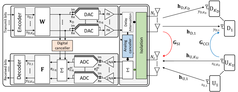
Figure 1: Full-duplex MU-MIMO system model with coarse quantization.

In UL perspective, UL user $k$ transmits $s_{{\sf U},k}\sim\mbox{$\mathcal{C}$}\mbox{$\mathcal{N}$}(0,P_{\sf U})$ for $k\in\{1,...,K_{\sf U}\}$, where $P_{\sf U}$ is a maximum transmit power of the UL user. We define ${\bf s}_{\sf U}=[s_{{\sf U},1},...,s_{{\sf U},K_{\sf U}}]^{\sf T}\in\mbox{$\mathbb{C}$}^{K_{\sf U}}$. According to [37], an UL analog received signal after analog SIC is then represented as

$${\bf r}_{\sf U}^{\sf ac}={\bf H}_{\sf U}{\bf s}_{\sf U}+{\bf G}_{\sf SI}{\bf x}_{\sf D,q}+{\bf n}_{\sf U},$$ (4)

where ${\bf H}_{\sf U}=\left[{{\bf h}_{{\sf U},1}},...,{{\bf h}_{{\sf U},K_{\sf U}}}\right]\in\mbox{$\mathbb{C}$}^{N_{r}\times K_{\sf U}}$ is a channel matrix from the UL users to the AP, ${\bf G}_{\sf SI}=\left[{\bf g}_{{\sf SI},1},...,{\bf g}_{{\sf SI},N_{t}}\right]\in\mbox{$\mathbb{C}$}^{N_{r}\times N_{t}}$ is a SI channel matrix, and ${\bf n}_{\sf U}\in\mbox{$\mathbb{C}$}^{N_{r}}$ is an UL noise vector, where ${\bf n}_{\sf U}\sim\mbox{$\mathcal{C}$}\mbox{$\mathcal{N}$}(\mathbf{0}_{N_{r}\times 1},\sigma_{\sf U}^{2}{\bf I}_{N_{r}})$ and each entry of ${\bf G}_{\sf SI}$ follows an independent and identically distributed (IID) $\mbox{$\mathcal{C}$}\mbox{$\mathcal{N}$}({0},\kappa_{\sf a})$. Here, $\kappa_{\sf a}$ is an analog SIC capability which includes passive and active cancellation. The UL channel vector for UL user $k$ is expressed as

$${\bf h}_{{\sf U},k}=\sqrt{\rho_{{\sf U},k}}\tilde{{\bf h}}_{{\sf U},k},$$ (5)

where $\rho_{{\sf U},k}$ and $\tilde{{\bf h}}_{{\sf U},k}$ are the UL path-loss and a small-scale fading vector with $\tilde{{\bf h}}_{{\sf U},k}\sim\mbox{$\mathcal{C}$}\mbox{$\mathcal{N}$}(\mathbf{0}_{N_{r}\times 1},{\bf C}_{{\sf U},k})$, respectively.

The UL analog received signal after analog SIC in (4) is quantized at ADCs. We denote the number of $k$th ADC bits as $b_{{\sf ADC},k}$. Using the AQNM, the quantized ${\bf r}_{\sf U}^{\sf ac}$ is given as

$$Q({\bf r}_{\sf U}^{\sf ac}) \approx{\bf r}_{\sf U,q}^{\sf ac}=\;\boldsymbol{\Phi}_{\alpha_{\sf ADC}}{\bf r}_{\sf U}^{\sf ac}+{\bf q}_{\sf ADC}$$

$$=\boldsymbol{\Phi}_{\alpha_{\sf ADC}}{\bf H}_{\sf U}{\bf s}_{\sf U}\!+\!\boldsymbol{\Phi}_{\alpha_{\sf ADC}}{\bf G}_{\sf SI}{\bf x}_{\sf D,q}\!+\!\boldsymbol{\Phi}_{\alpha_{\sf ADC}}{\bf n}_{\sf U}\!+\!{\bf q}_{\sf ADC},$$ (6)

where $\boldsymbol{\Phi}_{\alpha_{\sf ADC}}$ = $\mathrm{diag}\{\alpha_{\sf{ADC},1},...,\alpha_{{\sf ADC},N_{r}}\}\in\mbox{$\mathbb{C}$}^{N_{r}\times N_{r}}$ denotes a diagonal matrix of ADC quantization loss $\alpha_{{\sf ADC},n}$ which is defined as $\alpha_{{\sf ADC},n}=1-\beta_{{\sf ADC},n}\in(0,1)$ and ${\bf q}_{\sf{ADC}}\in\mbox{$\mathbb{C}$}^{N_{r}}$ is an ADC quantization noise vector. We assume $\beta_{{\sf ADC},n}$ can also be obtained as Table 1 in [36] for $b_{\sf ADC}\leq 5$ and $\beta_{{\sf ADC},n}\approx\frac{\pi\sqrt{3}}{2}2^{-2b_{{\sf ADC},n}}$ for $b_{\sf ADC}>5$. We also assume ${\bf q}_{\sf{ADC}}\sim\mbox{$\mathcal{C}$}\mbox{$\mathcal{N}$}(\mathbf{0}_{N_{r}\times 1},{\bf R}_{{\bf q}_{\sf{ADC}}{\bf q}_{\sf{ADC}}}({\bf W}))$ whose covariance matrix is computed as [35, 28]

$${\bf R}_{{\bf q}_{\sf{ADC}}{\bf q}_{\sf{ADC}}}({\bf W})=\boldsymbol{\Phi}_{\alpha_{\sf ADC}}\boldsymbol{\Phi}_{\beta_{\sf ADC}}\mathrm{diag}{\left\{\mbox{$\mathbb{E}$}\left[{\bf r}_{\sf U}^{\sf ac}({\bf r}_{\sf U}^{\sf ac})^{\sf H}\right]\right\}},$$ (7)

where

$$\mbox{$\mathbb{E}$}\left[{\bf r}_{\sf U}^{\sf ac}({\bf r}_{\sf U}^{\sf ac})^{\sf H}\right]= \;P_{\sf U}{\bf H}_{\sf U}{\bf H}_{\sf U}^{\sf H}+P_{\sf D}{\bf G}_{\sf SI}\boldsymbol{\Phi}_{\alpha_{\sf DAC}}{\bf W}{\bf W}^{\sf H}\boldsymbol{\Phi}_{\alpha_{\sf DAC}}^{\sf H}{\bf G}_{\sf SI}^{\sf H}$$

$$+{\bf G}_{\sf SI}{\bf R}_{{\bf q}_{\sf DAC}{\bf q}_{\sf DAC}}({\bf W}){\bf G}_{\sf SI}^{\sf H}+\sigma_{\sf U}^{2}{\bf I}_{N_{r}}.$$ (8)

Remark 1.

Since the received UL desired signal power $P_{\sf U}{\bf H}_{\sf U}{\bf H}_{\sf U}^{\sf H}$ and the UL noise power $\sigma_{\sf U}^{2}$ are much lower than the residual analog SI, the ADC quantization noise is dominated by the DL transmit power, the analog SIC capability, the number of ADC bits, and the precoder. In this regard, it is desirable to carefully determine the quantization resolution and design the precoder for 1) putting the residual analog signal power level down to the ADC dynamic range, 2) maintaining the ADC quantization noise power less than the received UL desired signal power, and 3) handling the quantization noise.

After digital SIC [37], the quantized signal in (6) becomes

$${\bf r}_{\sf U,q}\!=\!\boldsymbol{\Phi}_{\alpha_{\sf ADC}}{\bf H}_{\sf U}{\bf s}_{\sf U}\!+\!\sqrt{\kappa_{\sf d}}\boldsymbol{\Phi}_{\alpha_{\sf ADC}}\!{\bf G}_{\sf SI}{\bf x}_{\sf D,q}\!+\!\boldsymbol{\Phi}_{\alpha_{\sf ADC}}{\bf n}_{\sf U}\!+\!{\bf q}_{\sf ADC},$$ (9)

where $\kappa_{\sf d}$ denotes the digital SIC capability as shown in Fig. 2. The quantized signal vector in (9) is then combined as

$${\bf y}_{\sf U}= \;{\bf F}^{\sf H}\boldsymbol{\Phi}_{\alpha_{\sf ADC}}{\bf H}_{\sf U}{\bf s}_{\sf U}+\sqrt{\kappa_{\sf d}}{\bf F}^{\sf H}\boldsymbol{\Phi}_{\alpha_{\sf ADC}}{\bf G}_{\sf SI}\boldsymbol{\Phi}_{\alpha_{\sf DAC}}{\bf W}{\bf s}_{\sf D}$$

$$+\!\sqrt{\kappa_{\sf d}}{\bf F}^{\sf H}\boldsymbol{\Phi}_{\alpha_{\sf ADC}}{\bf G}_{\sf SI}{\bf q}_{\sf DAC}\!+\!{\bf F}^{\sf H}\boldsymbol{\Phi}_{\alpha_{\sf ADC}}{\bf n}_{\sf U}\!+\!{\bf F}^{\sf H}{\bf q}_{\sf ADC},$$ (10)

where ${\bf F}\in\mbox{$\mathbb{C}$}^{N_{r}\times K_{\sf U}}$ is a combining matrix whose $k$th column is ${\bf f}_{k}$. The received digital baseband signal for $k$th UL user is

$$y_{{\sf U},k}= \;{\bf f}_{k}^{\sf H}\boldsymbol{\Phi}_{\alpha_{\sf ADC}}{\bf h}_{{\sf U},k}s_{{\sf U},k}+\sum_{i=1,i\neq k}^{K_{\sf U}}{\bf f}_{k}^{\sf H}\boldsymbol{\Phi}_{\alpha_{\sf ADC}}{\bf h}_{{\sf U},i}s_{{\sf U},i}$$

$$+\sqrt{\kappa_{\sf d}}\sum_{i=1}^{K_{\sf D}}{\bf f}_{k}^{\sf H}\boldsymbol{\Phi}_{\alpha_{\sf ADC}}{\bf G}_{\sf SI}\boldsymbol{\Phi}_{\alpha_{\sf DAC}}{\bf w}_{i}s_{{\sf D},i}$$

$$+\sqrt{\kappa_{\sf d}}{\bf f}_{k}^{\sf H}\boldsymbol{\Phi}_{\alpha_{\sf ADC}}{\bf G}_{\sf SI}{\bf q}_{\sf DAC}\!+\!{\bf f}_{k}^{\sf H}\boldsymbol{\Phi}_{\alpha_{\sf ADC}}{\bf n}_{\sf U}\!+\!{\bf f}_{k}^{\sf H}{\bf q}_{\sf ADC}.$$ (11)

Returning to the DL perspective, we express a DL received signal vector at the DL users as

$${\bf y}_{\sf D}= \;{\bf H}^{\sf H}_{\sf D}{\bf x}_{\sf D,q}+{\bf G}_{\sf CCI}^{\sf H}{\bf s}_{\sf U}+{\bf n}_{\sf D}$$

$$= \;{\bf H}^{\sf H}_{\sf D}\boldsymbol{\Phi}_{\alpha_{\sf DAC}}{\bf W}{\bf s}_{\sf D}+{\bf H}^{\sf H}_{\sf D}{\bf q}_{\sf DAC}+{\bf G}_{\sf CCI}^{\sf H}{\bf s}_{\sf U}+{\bf n}_{\sf D},$$ (12)

where ${\bf H}_{\sf D}=\left[{{\bf h}_{{\sf D},1}},...,{{\bf h}_{{\sf D},K_{\sf D}}}\right]\in\mbox{$\mathbb{C}$}^{N_{t}\times K_{\sf D}}$ is a channel matrix from the AP to the DL users, ${\bf G}_{\sf CCI}=\left[{\bf g}_{{\sf CCI},1},...,{\bf g}_{{\sf CCI},K_{\sf D}}\right]\in\mbox{$\mathbb{C}$}^{K_{\sf U}\times K_{\sf D}}$ is a CCI channel matrix, and ${\bf n}_{\sf D}\in\mbox{$\mathbb{C}$}^{K_{\sf D}}$ is a DL noise vector. Similar to the UL channel, the $k$th DL user channel is

$${\bf h}_{{\sf D},k}=\sqrt{\rho_{{\sf D},k}}\tilde{{\bf h}}_{{\sf D},k},$$ (13)

where $\rho_{{\sf D},k}$ and $\tilde{{\bf h}}_{{\sf D},k}$ are the DL path-loss and a small-scale fading vector with $\tilde{{\bf h}}_{{\sf D},k}\sim\mbox{$\mathcal{C}$}\mbox{$\mathcal{N}$}({\bf 0}_{N_{t}\times 1},{\bf C}_{{\sf D},k})$, respectively. We assume that ${\bf g}_{{\sf CCI},k}=\sqrt{\rho_{{\sf CCI},k}}\tilde{{\bf g}}_{{\sf CCI},k}$ where $\rho_{{\sf CCI},k}$ denotes the CCI channel path-loss and $\tilde{{\bf g}}_{{\sf CCI},k}\sim\mbox{$\mathcal{C}$}\mbox{$\mathcal{N}$}(\mathbf{0}_{K_{\sf U}\times 1},{\bf I}_{K_{\sf U}})$, and ${\bf n}_{\sf D}\sim\mbox{$\mathcal{C}$}\mbox{$\mathcal{N}$}(\mathbf{0}_{K_{\sf D}\times 1},\sigma_{\sf D}^{2}{\bf I}_{K_{\sf D}})$. The received digital baseband signal for DL user $k$ is

$$y_{{\sf D},k}= \;{\bf h}_{{\sf D},k}^{\sf H}\boldsymbol{\Phi}_{\alpha_{\sf DAC}}{\bf w}_{k}s_{{\sf D},k}+\sum_{i=1,i\neq k}^{K_{\sf D}}{\bf h}_{{\sf D},k}^{\sf H}\boldsymbol{\Phi}_{\alpha_{\sf DAC}}{\bf w}_{i}s_{{\sf D},i}$$

$$+{\bf h}_{{\sf D},k}^{\sf H}{\bf q}_{\sf DAC}+{\bf g}_{{\sf CCI},k}^{\sf H}{\bf s}_{\sf U}+n_{{\sf D},k}.$$ (14)

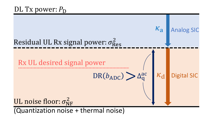
Figure 2: An illustrative example of the SIC procedure and the conditions of the ADC dynamic range and the received UL desired signal power.

III Analysis of ADC Dynamic Range and Quantization Noise in FD SISO System

In previous literature [18, 19, 20, 21, 25, 26, 27, 28], it has been demonstrated that using low-resolution quantizers increases the EE of the HD systems. Unlike HD systems, however, the strong residual analog SI challenges the use of low-resolution ADCs in the FD systems as discussed in Remark 1. Hence, we first aim to analyze the requirement on the ADCs for the considered FD system, thereby drawing system design insights. In the analysis, we assume that our system reduces to a scenario where the AP with a single transmit and a single receive antenna serves one UL user, i.e., a FD SISO system. We further assume infinite-resolution DACs at the AP.

Considering the average power, from (7) and (8), we first derive the average ADC quantization noise power as

$$\mathrm{\eta}_{\sf ADC}\!=\!\alpha_{\sf ADC}(1-\alpha_{\sf ADC})(P_{\sf U}\rho_{\sf U}+P_{\sf D}\kappa_{\sf a}+\sigma^{2}_{\sf U}).$$ (15)

We also compute the residual UL received signal power after analog SIC and UL noise floor after ADC quantization, respectively, as

$$\sigma^{2}_{\sf Res} =P_{\sf D}\kappa_{\sf a}+P_{\sf U}\rho_{\sf U}+\sigma^{2}_{\sf U},$$ (16)

$$\sigma^{2}_{\sf NF} =\mathrm{\eta}_{\sf ADC}+\sigma^{2}_{\sf U}\alpha^{2}_{\sf ADC}.$$ (17)

Based on (15), (16), and (17), we define the gap between the residual UL received analog signal power and the UL noise floor with the quantization noise in dB as shown in Fig. 2 as

$$\Delta_{\sf q}^{\sf ac}= \,10\mathrm{log}_{10}\sigma^{2}_{\sf Res}-10\mathrm{log}_{10}\sigma^{2}_{\sf NF}.$$ (18)

Now, considering $\beta_{\sf ADC}=\frac{\pi\sqrt{3}}{2}2^{-2b_{\sf ADC}}$ for any ADC quantization bits, we derive the following proposition:

Proposition 1.

Let us assume $\sigma^{2}_{\sf U}\ll P_{\sf D}\kappa_{\sf a}$ and $b_{\sf DAC}=\infty$. Then, for $\frac{P_{\sf D}\kappa_{\sf a}}{P_{\sf U}\rho_{\sf U}}\geq 3$, the received power of the UL desired signal achieves a higher power than the UL noise floor if the number of ADC bits satisfies the following condition:

$$b_{\sf ADC}\!>\!\frac{1}{2}\!\log_{2}\left(\!\frac{\pi}{2}\sqrt{\frac{3P_{\sf total}^{\sf Rx}}{4(P_{\sf UL}^{\sf Rx})^{2}}}\left(\sqrt{P_{\sf total}^{\sf Rx}}\!+\!\sqrt{P_{\sf total}^{\sf Rx}\!-\!4P_{\sf UL}^{\sf Rx}}\right)\!\right),$$ (19)

where $P_{\sf total}^{\sf Rx}=P_{\sf U}\rho_{\sf U}+P_{\sf D}\kappa_{\sf a}$ and $P_{\sf UL}^{\sf Rx}=P_{\sf U}\rho_{\sf U}$.

Proof.

We need to compute the following inequality with respect to the number of bits $b_{\sf ADC}$:

$$P_{\sf U}\rho_{\sf U}>\sigma^{2}_{\sf NF}.$$ (20)

With the assumption in this proposition, the UL received noise floor $\sigma^{2}_{\sf NF}$ in (17) reduces with $\alpha_{\sf DAC}=1$ to

$$\sigma^{2}_{\sf NF}\approx\alpha_{\sf ADC}(1-\alpha_{\sf ADC})(P_{\sf U}\rho_{\sf U}+P_{\sf D}\kappa_{\sf a}).$$ (21)

Now, recall $\alpha_{\sf ADC}=1-\frac{\pi\sqrt{3}}{2}2^{-2b_{\sf ADC}}$ which is particularly more accurate for $b_{\sf ADC}>5$. For analytical tractability, we assume $\alpha_{\sf ADC}=1-\frac{\pi\sqrt{3}}{2}2^{-2b_{\sf ADC}}$ for any $b_{\sf ADC}>0$. Then, applying $\alpha_{\sf ADC}=1-\frac{\pi\sqrt{3}}{2}2^{-2b_{\sf ADC}}$ to (21), the condition in (20) becomes

$$4^{2b_{\sf ADC}+1}P_{\sf U}\rho_{\sf U}\!>\!(\sqrt{3}\pi 2^{2b_{\sf ADC}+1}\!-\!3\pi^{2})(P_{\sf D}\kappa_{\sf a}\!+\!P_{\sf U}\rho_{\sf U}).$$ (22)

Solving (22) with respect to $b_{\sf ADC}$, we derive the condition (19). This completes the proof. ∎

Note that (19) is an increasing function of $P_{\sf total}^{\sf Rx}$ and a decreasing function of $P_{\sf UL}^{\sf Rx}$. Accordingly, the minimum of $b_{\sf ADC}$ is computed at $P_{\sf total}^{\sf Rx}=4P_{\sf UL}^{\sf Rx}$ since we need to have $P_{\sf total}^{\sf Rx}\geq 4P_{\sf UL}^{\sf Rx}$ to make $b_{\sf ADC}$ a real value. Hence, (19) has minimum value at $\frac{P_{\sf D}\kappa_{\sf a}}{P_{\sf U}\rho_{\sf U}}\geq 3$ (equal to $P_{\sf total}^{\sf Rx}=4P_{\sf UL}^{\sf Rx}$), which is $b_{\sf ADC}>0.72$. This indicates that the required number of bits can be reduced down to one bit when the UL desired signal power is comparable to the residual analog SI, which is typically not the case.

We further approximate (19) assuming $P^{\sf Rx}_{\sf total}\gg 4P^{\sf Rx}_{\sf UL}$ as

$$b_{\sf ADC}>\frac{1}{2}\log_{2}\frac{P^{\sf Rx}_{\sf total}}{P^{\sf Rx}_{\sf UL}}+\frac{1}{2}\log_{2}\frac{\pi\sqrt{3}}{2}.$$ (23)

This indicates that the required number of ADC bits in the FD system is logarithmically proportional to the ratio of the total received signal power and received UL desired signal power.

Now, we provide analysis on the ADC resolvability for the FD signal. The ADC dynamic range is approximated as [38]

$${\rm DR}(b_{\sf ADC})\!\approx\!20\log_{10}\left(\sqrt{\frac{3}{2}}2^{b_{\sf ADC}}\right).$$ (24)

Under the approximated dynamic range and quantization model, we have Proposition 2.

Proposition 2.

Let us assume $P_{\sf U}\rho_{\sf U}\ll P_{\sf D}\kappa_{\sf a}$. Then, under the same assumption as in Proposition 1 and considered system models, the ADC at the AP with FD can always resolve the quantization input signal, i.e., the following condition is always met:

$$\mathrm{DR}(b_{\sf ADC})>\Delta_{\sf q}^{\sf ac}.$$ (25)

Proof.

Based on (21), the gap between the residual UL received analog signal power and UL received noise floor in (18) reduces to (26) under the assumption of Proposition 2:

$$\Delta_{\sf q}^{\sf ac}\approx \,10\mathrm{log}_{10}(P_{\sf D}\kappa_{\sf a}+P_{\sf U}\rho_{\sf U})$$

$$-10\mathrm{log}_{10}(\alpha_{\sf ADC}(1-\alpha_{\sf ADC})(P_{\sf U}\rho_{\sf U}+P_{\sf D}\kappa_{\sf a}))$$

$$\stackrel{{\scriptstyle(a)}}{{\approx}} 10\mathrm{log}_{10}\left(\frac{1}{\alpha_{\sf ADC}(1-\alpha_{\sf ADC})}\right),$$ (26)

where $(a)$ follows from $P_{\sf U}\rho_{\sf U}\ll P_{\sf D}\kappa_{\sf a}$. Using (26) and the ADC dynamic range model in (24) with $\alpha_{\sf ADC}=1-\frac{\pi\sqrt{3}}{2}2^{-2b_{\sf ADC}}$, the condition in (25) becomes

$$20\log_{10}\left(\sqrt{\frac{3}{2}}2^{b_{\sf ADC}}\right)> -10\mathrm{log}_{10}\left(\pi\sqrt{3}\cdot 2^{-2b_{\sf ADC}-1}\right.$$

$$\left.\qquad\times(1-\pi\sqrt{3}\cdot 2^{-2b_{\sf ADC}-1})\right).$$ (27)

By rewriting (III) with respect to $b_{\sf ADC}$, we have

$$b_{\sf ADC}>\log_{2}3\pi-\frac{1}{2}\log_{2}(3\pi\sqrt{3}-4)-\frac{1}{2}\approx 0.9247.$$ (28)

Therefore, the condition in (25) is satisfied for any ADC bits $b_{\sf ADC}\in\mathbb{N}$. This completes the proof. ∎

TABLE I: ADC quantization noise $\eta_{\sf ADC}$, UL received signal range $\Delta_{\sf q}^{\sf ac}$, and ADC dynamic range DR$(b_{\sf ADC})$ for different analog SIC capability $\kappa_{\sf a}$, AP’s transmit power $P_{\sf D}$, and ADC/DAC bits $b$ with UL transmit power of $20\ \mathrm{dBm}$. All values are in $\rm dB$ or $\rm dBm$.

$\kappa_{\sf a}$	$b$	4 bits			5 bits			6 bits			7 bits			8 bits
	$P_{\sf D}$	${\eta}_{\sf ADC}$	$\Delta_{\sf q}^{\sf ac}$	DR	${\eta}_{\sf ADC}$	$\Delta_{\sf q}^{\sf ac}$	DR	${\eta}_{\sf ADC}$	$\Delta_{\sf q}^{\sf ac}$	DR	$\eta_{\sf ADC}$	$\Delta_{\sf q}^{\sf ac}$	DR	$\eta_{\sf ADC}$	$\Delta_{\sf q}^{\sf ac}$	DR
$-40$	$20$	$-42.80$	$22.80$	$25.84$	$-48.56$	$28.56$	$31.86$	$-54.31$	$34.31$	$37.88$	$-60.33$	$40.33$	$43.90$	$-66.35$	$46.35$	$49.92$
	$30$	$-32.80$	$22.80$		$-38.57$	$28.57$		$-44.31$	$34.31$		$-50.33$	$40.33$		$-56.35$	$46.35$
	$40$	$-22.80$	$22.80$		$-28.57$	$28.57$		$-34.31$	$34.31$		$-40.33$	$40.33$		$-46.35$	$46.35$
$-60$	$20$	$-62.73$	$22.73$	$25.84$	$-68.50$	$28.50$	$31.86$	$-74.24$	$34.24$	$37.88$	$-80.26$	$40.26$	$43.90$	$-86.28$	$46.28$	$49.92$
	$30$	$-52.78$	$22.78$		$-58.55$	$28.55$		$-64.30$	$34.30$		${\bf-70.32}$	$40.32$		$-76.34$	$46.34$
	$40$	$-42.80$	$22.80$		$-47.56$	$28.56$		$-54.31$	$34.31$		$-60.33$	$40.33$		$-66.35$	$46.35$

We note that the system assumptions such as $\sigma^{2}_{\sf U}\ll P_{\sf D}\kappa_{\sf a}$, $\frac{P_{\sf D}\kappa_{\sf a}}{P_{\sf U}\rho_{\sf U}}\geq 3$, and $P_{\sf U}\rho_{\sf U}\ll P_{\sf D}\kappa_{\sf a}$ are practical in most wireless systems. Then, we have the following remark:

Remark 2.

Based on Proposition 1 and Proposition 2, it is concluded that the ADC resolution for the FD system needs to be determined primarily by (19) to guarantee the UL signal quality as well as the ADC resolvability when DAC has no quantization error.

The finding described in Remark 2 is analogous to the numerical study in [33] in that analog SIC is particularly more important than the dynamic range. For the practical examination of Proposition 1, we provide the following example:

Example 1.

Considering an indoor communications, we set $P_{\sf D}=24\,\mathrm{dBm}$ and $P_{\sf U}=23\,\mathrm{dBm}$. We use $\kappa_{\sf a}=-60\,\mathrm{dB}$ which is typically the maximum analog SIC capability including passive and active cancellations [37]. We also set $\rho_{\sf U}=-90\,\mathrm{dBm}$ computed from the close-in (CI) path-loss model [39]. Then, the condition in (19) becomes $b_{\sf ADC}>5.87$.

Remark 3.

This result indicates that unlike the findings in HD low-resolution ADC systems that around $4$-bit ADC systems can provide the SE close to that of the infinite-bit ADC system [21, 22, 23, 24], a higher number of ADC bits, at least 6 bits, are needed for FD systems to avoid UL signals from drowning in the ADC quantization noise floor due to the strong residual analog SI. The required number of bits increases with higher $P_{\sf D}$ and lower analog SIC capability.

Furthermore, via simulations, numerical examples for the considered system with $N_{t}=1$ and $N_{r}=1$ are summarized in Table I. The simulation setup in Table I is as follows: the UL channel is randomly generated for each iteration of simulation, with the UL maximum transmit power of $20\,\mathrm{dBm}$. In the UL channel modeling, the UL path-loss and small-scale fading factor are derived by the one-ring channel model [40] and the CI path-loss model [39], respectively. Moreover, the UL user is randomly distributed within a circle with a radius of 4$\,\mathrm{m}$, where the circle is located 15$\,\mathrm{m}$ away from the AP. We ignore the thermal noise in this example. Then, the ADC quantization noise power $\eta_{\sf ADC}$ and the UL received signal power range $\Delta_{\sf q}^{\sf ac}$ are averaged. DR is computed from (24). From Table I, one can infer the minimum number of ADC bits required for guaranteeing the UL desired signal quality in FD systems.

For instance, let us also consider $\rho_{\sf U}=-90\,\mathrm{dBm}$ UL path-loss. Then, with $\kappa_{\sf a}=-60\,\mathrm{dB}$ and $P_{\sf D}=30\,\mathrm{dBm}$, the derived condition (19) gives $b_{\sf ADC}>7.37$. Similarly, from Table I, at least $b_{\sf ADC}\geq 7$ is required to make the average UL received signal power $P_{\sf U}\rho_{\sf U}=-70\,\mathrm{dBm}$ larger than the quantization noise floor $\eta_{\sf ADC}$ which turns out to be $\eta_{\sf ADC}=-70.32\,\mathrm{dBm}$. In addition, we note that $\mathrm{DR}$ is always larger than $\Delta_{\sf q}^{\sf ac}$ regardless of the system parameters, which guarantees ADC resolvability. Both the observations align with the findings in Proposition 1 and Proposition 2.

The derived findings highlight that unlike the infinite-resolution ADC FD systems where the SI can be almost fully cancelled, it is imperative to exert control over the residual analog SI in the low-resolution ADC FD systems. Consequently, the FD MU-MIMO system design under coarse quantization requires to jointly consider beamforming and its impact to the quantization noise due to the SI. In other words, the FD MU-MIMO beamformer needs to not only maximize the DL signal-to-interference-plus-noise ratio (SINR), but also mitigate the SI under coarse quantization.

IV Sum Spectral Efficiency Maximization

Motivated by the insights obtained in Section III, we develop an advanced FD MU-MIMO beamforming algorithm that considers the effect of the SI as well as IUI, CCI and quantization noise for maximizing the UL and DL sum SE. To this end, we first formulate the sum SE maximization problem and then split the problem into two sub-problems. In each problem, either precoder or combiner is optimized. In particular, the precoder is designed by incorporating the SI jointly with the quantization noise.

IV-A Performance Metric and Problem Formulation

For the FD MU-MIMO system described in Section II, we compute the SEs of the DL and UL users as (29) and (30), respectively, which are shown at the top of next page,

$$R_{{\sf D},k}({\bf W})=\mathrm{log}_{2}\left(1+\frac{|{\bf h}_{{\sf D},k}^{\sf H}\boldsymbol{\Phi}_{\alpha_{\sf DAC}}{\bf w}_{k}|^{2}P_{\sf D}}{\sum_{i=1,i\neq k}^{K_{\sf D}}|{\bf h}_{{\sf D},k}^{\sf H}\boldsymbol{\Phi}_{\alpha_{\sf DAC}}{\bf w}_{i}|^{2}P_{\sf D}+\mathrm{QN}_{{\sf DAC},k}+I_{{\sf CCI},k}+\sigma_{\sf D}^{2}}\right).$$ (29)

 

$$R_{{\sf U},k}({\bf W},{\bf F})=\mathrm{log}_{2}\left(1+\frac{|{\bf f}_{k}^{\sf H}\boldsymbol{\Phi}_{\alpha_{\sf ADC}}{\bf h}_{{\sf U},k}|^{2}P_{\sf U}}{\sum_{i=1,i\neq k}^{K_{\sf U}}|{\bf f}_{k}^{\sf H}\boldsymbol{\Phi}_{\alpha_{\sf ADC}}{\bf h}_{{\sf U},i}|^{2}P_{\sf U}+\mathrm{QN}_{{\sf ADC},k}+I_{{\sf SI},k}+\|{\bf f}_{k}^{\sf H}\boldsymbol{\Phi}_{\alpha_{\sf ADC}}\|^{2}\sigma_{\sf U}^{2}}\right).$$ (30)

 

where

$${I}_{{\sf CCI},k} =\,\|{\bf g}_{{\sf CCI},k}\|^{2}P_{\sf U},$$ (31)

$$I_{{\sf SI},k} =\,\kappa_{\sf d}\sum_{i=1}^{K_{\sf D}}|{\bf f}_{k}^{\sf H}\boldsymbol{\Phi}_{\alpha_{\sf ADC}}{\bf G}_{\sf SI}\boldsymbol{\Phi}_{\alpha_{\sf DAC}}{\bf w}_{i}|^{2}P_{\sf D}$$

$$+\kappa_{\sf d}{\bf f}_{k}^{\sf H}\boldsymbol{\Phi}_{\alpha_{\sf ADC}}{\bf G}_{\sf SI}{\bf R}_{{\bf q}_{\sf{DAC}}{\bf q}_{\sf{DAC}}}({\bf W}){\bf G}_{\sf SI}^{\sf H}\boldsymbol{\Phi}_{\alpha_{\sf ADC}}^{\sf H}{\bf f}_{k},$$ (32)

$$\mathrm{QN}_{{\sf DAC},k} =\;{\bf h}_{{\sf D},k}^{\sf H}{\bf R}_{{\bf q}_{\sf{DAC}}{\bf q}_{\sf{DAC}}}({\bf W}){\bf h}_{{\sf D},k},$$ (33)

$$\mathrm{QN}_{{\sf ADC},k} =\;{\bf f}_{k}^{\sf H}{\bf R}_{{\bf q}_{\sf{ADC}}{\bf q}_{\sf{ADC}}}({\bf W}){\bf f}_{k}.$$ (34)

In addition, the DL transmit power is computed as

$$\mathrm{Tr}\left(\mbox{$\mathbb{E}$}\left[{\bf x}_{\sf D,q}{\bf x}_{\sf D,q}^{\sf H}\right]\right)$$

$$=\mathrm{Tr}\bigg{(}P_{\sf D}\boldsymbol{\Phi}_{\alpha_{\sf DAC}}{\bf W}{\bf W}^{\sf H}\boldsymbol{\Phi}_{\alpha_{\sf DAC}}^{\sf H}+\boldsymbol{\Phi}_{\alpha_{\sf DAC}}\boldsymbol{\Phi}_{\beta_{\sf DAC}}\mathrm{diag}{\left\{P_{\sf D}{\bf W}{\bf W}^{\sf H}\right\}}\bigg{)}$$

$$\overset{(a)}{=}\mathrm{Tr}\left(P_{\sf D}\boldsymbol{\Phi}_{\alpha_{\sf DAC}}{\bf W}{\bf W}^{\sf H}\right),$$ (35)

where $(a)$ is derived from the relationship of between $\boldsymbol{\Phi}_{\alpha_{\sf DAC}}$ and $\boldsymbol{\Phi}_{\beta_{\sf DAC}}$, i.e., $\boldsymbol{\Phi}_{\alpha_{\sf DAC}}+\boldsymbol{\Phi}_{\beta_{\sf DAC}}={\bf I}_{N_{t}}$, and the trace property.

Then, we formulate a maximum total sum SE problem as

$$\underset{{\bf W},{\bf F}}{\mathrm{maximize}} \;\sum_{k=1}^{K_{\sf D}}R_{{\sf D},k}({\bf W})+\sum_{k=1}^{K_{\sf U}}R_{{\sf U},k}({\bf W};{\bf F})$$ (36)

$$\mathrm{subject\;to} \;\mathrm{Tr}\left(\boldsymbol{\Phi}_{\alpha_{\sf DAC}}{\bf W}{\bf W}^{\sf H}\right)\leq 1,$$ (37)

where (37) is a transmit power constraint at the AP. We assume that the UL and DL channel state information (CSI) are perfectly known at the AP. It is important to find the precoding and combining solutions that effectively incorporate the quantization noise, SI, and CCI for maximizing the sum SE. Unfortunately, solving the optimization problem (36) is significantly challenging due to the presence of the CCI, residual SI, and quantization error. In particular, the residual SI and quantization error are coupled with the precoder and combiner, making the problem more difficult to solve. To resolve these challenges, we divide the problem into two sub-problems each of which corresponds to the precoder optimization or the combiner optimization.

IV-B Precoder Optimization

Let us consider the sub-problem associated with the precoder ${\bf W}$ optimization for a fixed combiner ${\bf F}$ from the problem in (36). Notwithstanding the fixed combiner, (36) is still non-convex and thus, it is infeasible to find a global optimal solution. Accordingly, we convert the problem in (36) into a more tractable form and derive a first-order optimality condition to identify local optimal solutions.

IV-B1 Problem Reformulation

We rewrite the problem to be a GPI-friendly form to utilize the GPI method [41]; the DAC quantization noise-related term in (33) is reformulated as

$${\mathrm{QN}_{{\sf DAC},k}} =P_{\sf D}{\bf h}_{{\sf D},k}^{\sf H}\boldsymbol{\Phi}_{\alpha_{\sf DAC}}\boldsymbol{\Phi}_{\beta_{\sf DAC}}\mathrm{diag}{\left\{\sum_{i=1}^{K_{\sf D}}{\bf w}_{i}{\bf w}^{\sf H}_{i}\!\right\}}{\bf h}_{{\sf D},k}$$

$$=P_{\sf D}\sum_{i=1}^{K_{\sf D}}\!{\bf w}^{\sf H}_{i}\boldsymbol{\Phi}_{\alpha_{\sf DAC}}\boldsymbol{\Phi}_{\beta_{\sf DAC}}\mathrm{diag}{\left\{{\bf h}_{{\sf D},k}{\bf h}_{{\sf D},k}^{\sf H}\right\}}{\bf w}_{i}.$$ (38)

Applying (38) to (29) with simplification, we have the reformulated SE of DL user $k$ in (39) at the top of next page.

$$R_{{\sf D},k}^{\sf ref}({\bf W})=\mathrm{log}_{2}\left(1+\frac{|{\bf h}_{{\sf D},k}^{\sf H}\boldsymbol{\Phi}_{\alpha_{\sf DAC}}{\bf w}_{k}|^{2}}{\sum_{i=1,i\neq k}^{K_{\sf D}}|{\bf h}_{{\sf D},k}^{\sf H}\boldsymbol{\Phi}_{\alpha_{\sf DAC}}{\bf w}_{i}|^{2}+\sum_{i=1}^{K_{\sf D}}\!{\bf w}^{\sf H}_{i}\boldsymbol{\Phi}_{\alpha_{\sf DAC}}\boldsymbol{\Phi}_{\beta_{\sf DAC}}\mathrm{diag}{\left\{{\bf h}_{{\sf D},k}{\bf h}_{{\sf D},k}^{\sf H}\right\}}{\bf w}_{i}+\|{\bf g}_{{\sf CCI},k}\|^{2}\frac{P_{\sf U}}{P_{\sf D}}+\frac{\sigma_{\sf D}^{2}}{P_{\sf D}}}\right).$$ (39)

 

Next, we define a weighted precoding vector as

$${\bf v}_{k}=\boldsymbol{\Phi}_{\alpha_{\sf DAC}}^{1/2}{\bf w}_{k},$$ (40)

where ${\bf v}_{k}\in\mbox{$\mathbb{C}$}^{N_{t}}$ for $k\in\{1,...,K_{\sf D}\}$. Stacking ${\bf v}_{k}$, we have

$$\bar{{\bf v}}=\left[{\bf v}_{1}^{\sf{T}},{\bf v}_{2}^{\sf{T}},...,{\bf v}_{K_{\sf D}}^{\sf{T}}\right]^{\sf T}\in\mbox{$\mathbb{C}$}^{N_{t}K_{\sf D}}.$$ (41)

We assume $\|\bar{{\bf v}}\|^{2}=1$ which implies using maximum transmit power $P_{\sf D}$. Using $\|\bar{\bf v}\|^{2}=1$, we rewrite the CCI and noise power in (39) that are the precoder-independent term as

$$\|{\bf g}_{{\sf CCI},k}\|^{2}\frac{P_{\sf U}}{P_{\sf D}}+\frac{\sigma_{\sf D}^{2}}{P_{\sf D}}=\bar{\bf v}^{\sf H}\left(\|{\bf g}_{{\sf CCI},k}\|^{2}\frac{P_{\sf U}}{P_{\sf D}}+\frac{\sigma_{\sf D}^{2}}{P_{\sf D}}\right)\bar{\bf v}.$$ (42)

Let ${\bf M}_{k}$ be

$${\bf M}_{k}\!=\!(\boldsymbol{\Phi}_{\alpha_{\sf DAC}}^{1/2})^{\sf H}{\bf h}_{{\sf D},k}{\bf h}_{{\sf D},k}^{\sf H}\boldsymbol{\Phi}_{\alpha_{\sf DAC}}^{1/2}+\boldsymbol{\Phi}_{\beta_{\sf DAC}}\mathrm{diag}{\left\{{\bf h}_{{\sf D},k}{\bf h}_{{\sf D},k}^{\sf H}\right\}}.$$ (43)

Then, using (40), (41), (42), and (43), we can represent $R^{\sf ref}_{{\sf D},k}({\bf W})$ in (39) as a Rayleigh quotient form in logarithm:

$$\gamma_{{\sf D},k}(\bar{\bf v})=\mathrm{log}_{2}\left(\frac{\bar{{\bf v}}^{\sf H}{\bf A}_{k}\bar{{\bf v}}}{\bar{{\bf v}}^{\sf H}{\bf B}_{k}\bar{{\bf v}}}\right),$$ (44)

where ${\bf A}_{k}\in\mbox{$\mathbb{C}$}^{N_{t}K_{\sf D}\times N_{t}K_{\sf D}}$ and ${\bf B}_{k}\in\mbox{$\mathbb{C}$}^{N_{t}K_{\sf D}\times N_{t}K_{\sf D}}$ are

$${\bf A}_{k}=\;\mathbf{I}_{K_{\sf D}}\otimes{\bf M}_{k}+\left(\|{\bf g}_{{\sf CCI},k}\|^{2}\frac{P_{\sf U}}{P_{\sf D}}+\!\frac{\sigma_{\sf D}^{2}}{P_{\sf D}}\right){\bf I}_{N_{t}K_{\sf D}},$$ (45)

$${\bf B}_{k}={\bf A}_{k}-\mathrm{diag}\left\{{\bf e}_{k}^{N_{t}}\right\}\otimes(\boldsymbol{\Phi}_{\alpha_{\sf DAC}}^{1/2})^{\sf H}{\bf h}_{{\sf D},k}{\bf h}_{{\sf D},k}^{\sf H}\boldsymbol{\Phi}_{\alpha_{\sf DAC}}^{1/2}.$$ (46)

Likewise, to rewrite the UL SE, we re-express $I_{{\sf SI},k}$ in (32) as

$$\bar{I}_{{\sf SI},k}=\frac{I_{{\sf SI},k}}{P_{\sf U}}=\kappa_{\sf d}\frac{P_{\sf D}}{P_{\sf U}}\sum_{i=1}^{K_{\sf D}}{\bf w}_{i}^{\sf H}\Psi_{{\sf SI},k}{\bf w}_{i},$$ (47)

where

$$\Psi_{{\sf SI},k}= \,\boldsymbol{\Phi}_{\alpha_{\sf DAC}}^{\sf H}{\bf G}_{\sf SI}^{\sf H}\boldsymbol{\Phi}_{\alpha_{\sf ADC}}^{\sf H}{\bf f}_{k}{\bf f}_{k}^{\sf H}\boldsymbol{\Phi}_{\alpha_{\sf ADC}}{\bf G}_{\sf SI}\boldsymbol{\Phi}_{\alpha_{\sf DAC}}$$

$$+\,\boldsymbol{\Phi}_{\alpha_{\sf DAC}}\boldsymbol{\Phi}_{\beta_{\sf DAC}}\mathrm{diag}{\left\{{\bf G}_{\sf SI}^{\sf H}\boldsymbol{\Phi}_{\alpha_{\sf ADC}}^{\sf H}{\bf f}_{k}{\bf f}_{k}^{\sf H}\boldsymbol{\Phi}_{\alpha_{\sf ADC}}{\bf G}_{\sf SI}\right\}}.$$ (48)

We also rewrite the ADC quantization-related term in (34) as

$$\bar{\mathrm{QN}}_{{\sf ADC},k} =\frac{\mathrm{QN}_{{\sf ADC},k}}{P_{\sf U}}=\sum_{i=1}^{K_{\sf U}}{\bf h}_{{\sf U},i}^{\sf H}\boldsymbol{\Phi}_{\alpha_{\sf ADC}}\boldsymbol{\Phi}_{\beta_{\sf ADC}}\mathrm{diag}\left\{{\bf f}_{k}{\bf f}_{k}^{\sf H}\right\}{\bf h}_{{\sf U},i}$$

$$+\frac{P_{\sf D}}{P_{\sf U}}\sum_{i=1}^{K_{\sf D}}{\bf w}_{i}^{\sf H}\Psi_{{\sf QN},k}{\bf w}_{i}\!+\!\frac{\sigma_{\sf U}^{2}}{P_{\sf U}}{\bf f}_{k}^{\sf H}\boldsymbol{\Phi}_{\alpha_{\sf ADC}}\boldsymbol{\Phi}_{\beta_{\sf ADC}}{\bf f}_{k},$$ (49)

where

$$\Psi_{{\sf QN},k}=\;\boldsymbol{\Phi}_{\alpha_{\sf DAC}}^{\sf H}{\bf G}_{\sf SI}^{\sf H}\boldsymbol{\Phi}_{\alpha_{\sf ADC}}\boldsymbol{\Phi}_{\beta_{\sf ADC}}\mathrm{diag}{\left\{{\bf f}_{k}{\bf f}_{k}^{\sf H}\right\}}{\bf G}_{\sf SI}\boldsymbol{\Phi}_{\alpha_{\sf DAC}}$$

$$\ +\boldsymbol{\Phi}_{\alpha_{\sf DAC}}\boldsymbol{\Phi}_{\beta_{\sf DAC}}\mathrm{diag}{\left\{{\bf G}_{\sf SI}^{\sf H}\boldsymbol{\Phi}_{\alpha_{\sf ADC}}\boldsymbol{\Phi}_{\beta_{\sf ADC}}\mathrm{diag}{\left\{{\bf f}_{k}{\bf f}_{k}^{\sf H}\right\}}{\bf G}_{\sf SI}\right\}}.$$ (50)

We note that the SI is included in the attenuated SI term $\Psi_{{\sf SI},k}$ in (48) and the ADC quantization noise-related term $\Psi_{{\sf QN},k}$ in (50). Accordingly, the precoders ${\bf w}_{i}$ need to be designed to mitigate $\Psi_{{\sf SI},k}$ and $\Psi_{{\sf QN},k}$. Since the digital SIC is not applied to $\Psi_{{\sf QN},k}$, it is more critical in low-resolution ADC systems to reduce $\Psi_{{\sf QN},k}$. Applying (47) and (49) to (30), we also reorganize the UL SE in (51) at the top of the next page.

$$R_{{\sf U},k}^{\sf ref}({\bf W},{\bf F})=\mathrm{log_{2}}{\left(1+\frac{|{\bf f}_{k}^{\sf H}\boldsymbol{\Phi}_{\alpha_{\sf ADC}}{\bf h}_{{\sf U},k}|^{2}}{\sum_{i=1,i\neq k}^{K_{\sf U}}|{\bf f}_{k}^{\sf H}\boldsymbol{\Phi}_{\alpha_{\sf ADC}}{\bf h}_{{\sf U},i}|^{2}+\bar{\mathrm{QN}}_{{\sf ADC},k}+\bar{I}_{{\sf SI},k}+\|{\bf f}_{k}^{\sf H}\boldsymbol{\Phi}_{\alpha_{\sf ADC}}\|^{2}\frac{\sigma_{\sf U}^{2}}{P_{\sf U}}}\right)}.$$ (51)

 

Similar to the DL SE in (44), defining ${\bf N}_{k}$ as

$${\bf N}_{k}= \;\frac{P_{\sf D}}{P_{\sf U}}\boldsymbol{(\Phi}_{\alpha_{\sf DAC}}^{-1/2})^{\sf H}\bigg{(}\Psi_{{\sf QN},k}+\kappa_{\sf d}\Psi_{{\sf SI},k}\bigg{)}\boldsymbol{\Phi}_{\alpha_{\sf DAC}}^{-1/2},$$ (52)

and using (40), (41) with $\|\bar{{\bf v}}\|^{2}=1$, we also rewrite $R^{\sf ref}_{{\sf U},k}({\bf W},{\bf F})$ in (51) as a Rayleigh quotient form in logarithm:

$$\gamma_{{\sf U},k}(\bar{\bf v};{\bf F})=\mathrm{log}_{2}\left(\frac{\bar{{\bf v}}^{\sf H}{\bf C}_{k}\bar{{\bf v}}}{\bar{{\bf v}}^{\sf H}{\bf D}_{k}\bar{{\bf v}}}\right),$$ (53)

where ${\bf C}_{k}\in\mbox{$\mathbb{C}$}^{N_{t}K_{\sf D}\times N_{t}K_{\sf D}}$ and ${\bf D}_{k}\in\mbox{$\mathbb{C}$}^{N_{t}K_{\sf D}\times N_{t}K_{\sf D}}$ are

$${\bf C}_{k}=\mathbf{I}_{K_{\sf D}}\otimes{\bf N}_{k}+\phi_{k}{\bf I}_{N_{t}K_{\sf D}},$$ (54)

$${\bf D}_{k}={\bf C}_{k}-\mathrm{diag}\{{\bf e}_{k}^{N_{t}}\}\otimes|{\bf f}_{k}^{\sf H}\boldsymbol{\Phi}_{\alpha_{\sf ADC}}{\bf h}_{{\sf U},k}|^{2}.$$ (55)

Here $\phi_{k}$ is the precoder-independent term of (51) and given with some simplification using $\boldsymbol{\Phi}_{\alpha_{\sf ADC}}={\bf I}_{N_{r}}-\boldsymbol{\Phi}_{\beta_{\sf ADC}}$ as

$$\phi_{k}= \sum_{i=1}^{K_{\sf U}}|{\bf f}_{k}^{\sf H}\boldsymbol{\Phi}_{\alpha_{\sf ADC}}{\bf h}_{{\sf U},i}|^{2}\!+\!\sum_{i=1}^{K_{\sf U}}{\bf h}_{{\sf U},i}^{\sf H}\boldsymbol{\Phi}_{\alpha_{\sf ADC}}\boldsymbol{\Phi}_{\beta_{\sf ADC}}\mathrm{diag}\left\{{\bf f}_{k}{\bf f}_{k}^{\sf H}\right\}{\bf h}_{{\sf U},i}$$

$$+{\bf f}_{k}^{\sf H}\boldsymbol{\Phi}_{\alpha_{\sf ADC}}{\bf f}_{k}\frac{\sigma_{\sf U}^{2}}{P_{\sf U}}.$$ (56)

Based on (40), (44) and (53), the optimization problem in (36) is reformulated with fixed ${\bf F}$ as

$$\underset{\bar{{\bf v}}}{\mathrm{maximize}} \;R_{\Sigma}(\bar{\bf v})=\sum_{k=1}^{K_{\sf D}}\gamma_{{\sf D},k}(\bar{\bf v})+\sum_{k=1}^{K_{\sf U}}\gamma_{{\sf U},k}(\bar{\bf v};{\bf F})$$ (57)

$$\mathrm{subject\;to} \;\|\bar{{\bf v}}\|^{2}=1.$$ (58)

IV-B2 Precoding Algorithm

It is noticed that the non-convexity still remains in the reformulated problem (57). To address this challenge, we derive the first-order optimality condition of (57) to identify stationary points of the problem.

Lemma 1.

The first-order optimality condition of (57) is represented in the generalized eigenvalue problem as

$${\bf B}^{-1}_{\sf KKT}(\bar{{\bf v}}){\bf A}_{\sf KKT}(\bar{{\bf v}})\bar{{\bf v}}=\lambda(\bar{{\bf v}})\bar{{\bf v}},$$ (59)

where

$${\bf A}_{\sf KKT}(\bar{{\bf v}})= \left[\sum_{k=1}^{\sf K_{\sf D}}\left(\frac{{\bf A}_{k}}{\bar{{\bf v}}^{\sf H}{\bf A}_{k}\bar{{\bf v}}}\right)+\sum_{k=1}^{\sf K_{\sf U}}\left(\frac{{\bf C}_{k}}{\bar{{\bf v}}^{\sf H}{\bf C}_{k}\bar{{\bf v}}}\right)\right]\lambda_{\sf num}(\bar{{\bf v}}),$$ (60)

$${\bf B}_{\sf KKT}(\bar{{\bf v}})= \left[\sum_{k=1}^{\sf K_{\sf D}}\left(\frac{{\bf B}_{k}}{\bar{{\bf v}}^{\sf H}{\bf B}_{k}\bar{{\bf v}}}\right)+\sum_{k=1}^{\sf K_{\sf U}}\left(\frac{{\bf D}_{k}}{\bar{{\bf v}}^{\sf H}{\bf D}_{k}\bar{{\bf v}}}\right)\right]\lambda_{\sf den}(\bar{{\bf v}}),$$ (61)

$$\lambda(\bar{{\bf v}})= \;\prod_{k=1}^{K_{\sf D}}\left(\frac{\bar{{\bf v}}^{\sf H}{\bf A}_{k}\bar{{\bf v}}}{\bar{{\bf v}}^{\sf H}{\bf B}_{k}\bar{{\bf v}}}\right)\prod_{k=1}^{K_{\sf U}}\left(\frac{\bar{{\bf v}}^{\sf H}{\bf C}_{k}\bar{{\bf v}}}{\bar{{\bf v}}^{\sf H}{\bf D}_{k}\bar{{\bf v}}}\right),$$ (62)

and $\lambda_{\sf num}(\bar{{\bf v}})$ and $\lambda_{\sf den}(\bar{{\bf v}})$ can be any functions that satisfy $\lambda(\bar{{\bf v}})=\lambda_{\sf num}(\bar{{\bf v}})/\lambda_{\sf den}(\bar{{\bf v}})$.

Proof.

See Appendix A. ∎

It is important to note that the eigenvalue $\lambda(\bar{\bf v})$ is related with the objective function in (57) as $R_{\Sigma}(\bar{{\bf v}})=\log_{2}\lambda(\bar{\bf v})$. According to Lemma 1, the stationary points satisfy (59) as an eigenvector of ${\bf B}^{-1}_{\sf KKT}(\bar{{\bf v}}){\bf A}_{\sf KKT}(\bar{{\bf v}})$, and the corresponding eigenvalue is $\lambda(\bar{\bf v})$ which is proportional to the sum SE $R_{\Sigma}(\bar{\bf v})$. This interpretation implies that we need to find the principal eigenvector of the problem (59) for maximizing $R_{\Sigma}(\bar{\bf v})$, and the principal eigenvector is the precoding vector on one of the stationary points. Specifically, the first-order optimality condition (59) is equivalent to the NEPv, and we leverage the GPI method to find its principal eigenvector.

We present the sum SE maximization precoding algorithm in Algorithm 1. The key steps of Algorithm 1 are as follows: we first initialize the stacked precoding vectors $\bar{{\bf v}}^{(0)}$ using a conventional linear precoder such as MRT, ZF, and regularized ZF (RZF). At each iteration $n$, we build the matrices ${\bf A}_{\sf KKT}(\bar{{\bf v}}^{(n-1)})$ and ${\bf B}_{\sf KKT}(\bar{{\bf v}}^{(n-1)})$ according to $\eqref{eq:A_KKT}$ and $\eqref{eq:B_KKT}$. Then, we compute $\bar{{\bf v}}^{(n)}$ as $\bar{{\bf v}}^{(n)}$ = ${\bf B}_{\sf KKT}^{-1}(\bar{{\bf v}}^{(n-1)}){\bf A}_{\sf KKT}(\bar{{\bf v}}^{(n-1)})\bar{{\bf v}}^{(n-1)}$ followed by normalization $\bar{{\bf v}}^{(n)}=\bar{{\bf v}}^{(n)}/\|\bar{{\bf v}}^{(n)}\|$. This normalization ensures the transmit power constraint. We repeat this process until the stopping criterion $\|\bar{{\bf v}}^{(n)}-\bar{{\bf v}}^{(n-1)}\|<\varepsilon_{\sf{\bf v}}$ is met, where $\varepsilon_{\sf{\bf v}}>0$ denotes a tolerance level or until the iteration count reaches the maximum count $n>n_{\sf max}$.

1 initialize: $\bar{{\bf v}}^{(0)}$

2 Set the iteration count $n=1.$

3 while $\|\bar{{\bf v}}^{(n)}-\bar{{\bf v}}^{(n-1)}\|>\varepsilon_{{\bf v}}$ and $n\leq n_{\sf max}$ do

4       Build matrix ${\bf A}_{\sf KKT}(\bar{{\bf v}}^{(n-1)})$ in (60).

5       Build matrix ${\bf B}_{\sf KKT}(\bar{{\bf v}}^{(n-1)})$ in (61).

6       Compute $\bar{{\bf v}}^{(n)}$ = ${\bf B}_{\sf KKT}^{-1}(\bar{{\bf v}}^{(n-1)}){\bf A}_{\sf KKT}(\bar{{\bf v}}^{(n-1)})\bar{{\bf v}}^{(n-1)}.$

7       Normalize $\bar{{\bf v}}^{(n)}=\bar{{\bf v}}^{(n)}/\|\bar{{\bf v}}^{(n)}\|.$

8       $n\leftarrow n+1.$

9      

10$\bar{{\bf v}}^{\star}\leftarrow\bar{{\bf v}}^{(n)}.$

return $\bar{{\bf v}}^{\star}$

Algorithm 1 Precoder Design

IV-C Combiner Optimization

Regarding the combiner optimization, it is known that the MMSE equalizer maximizes the received SINR. Accordingly, we build a quantization-aware linear MMSE (qMMSE) equalizer with the derived precoder from Algorithm 1. Let ${\bf z}_{k}$ be the sum of the IUI including the SI and UL noise including the quantization noise before passing through ${\bf F}$, i.e.,

$${\bf z}_{k}= \sum_{i=1,i\neq k}^{K_{\sf U}}\boldsymbol{\Phi}_{\alpha_{\sf ADC}}{\bf h}_{{\sf U},i}s_{{\sf U},i}+\sqrt{\kappa_{\sf d}}\sum_{i=1}^{K_{\sf D}}\boldsymbol{\Phi}_{\alpha_{\sf ADC}}{\bf G}_{\sf SI}\boldsymbol{\Phi}_{\alpha_{\sf DAC}}{\bf w}_{i}s_{{\sf D},i}$$

$$+\sqrt{\kappa_{\sf d}}\boldsymbol{\Phi}_{\alpha_{\sf ADC}}{\bf G}_{\sf SI}{\bf q}_{\sf DAC}+{\bf q}_{\sf ADC}+\boldsymbol{\Phi}_{\alpha_{\sf ADC}}{\bf n}_{\sf U}.$$ (63)

Using (63), the combining vector is defined as

$${\bf f}_{k}={\bf K}_{{\bf z}_{k}}^{-1}{\bf h}_{{\sf U},k},$$ (64)

where

$${\bf K}_{{\bf z}_{k}}=\; \mbox{$\mathbb{E}$}\left[{\bf z}_{k}{\bf z}_{k}^{\sf H}\right]=\;P_{\sf U}\sum_{i=1,i\neq k}^{K_{\sf U}}\boldsymbol{\Phi}_{\alpha_{\sf ADC}}{\bf h}_{{\sf U},i}{\bf h}_{{\sf U},i}^{\sf H}\boldsymbol{\Phi}_{\alpha_{\sf ADC}}^{\sf H}$$

$$+\kappa_{\sf d}P_{\sf D}\sum_{i=1}^{K_{\sf D}}\boldsymbol{\Phi}_{\alpha_{\sf ADC}}{\bf G}_{\sf SI}\boldsymbol{\Phi}_{\alpha_{\sf DAC}}{\bf w}_{i}{\bf w}_{i}^{\sf H}\boldsymbol{\Phi}_{\alpha_{\sf DAC}}^{\sf H}{\bf G}_{\sf SI}^{\sf H}\boldsymbol{\Phi}_{\alpha_{\sf ADC}}^{\sf H}$$

$$+\kappa_{\sf d}\boldsymbol{\Phi}_{\alpha_{\sf ADC}}{\bf G}_{\sf SI}{\bf R}_{{\bf q}_{\sf{DAC}}{\bf q}_{\sf{DAC}}}{\bf G}_{\sf SI}^{\sf H}\boldsymbol{\Phi}_{\alpha_{\sf ADC}}^{\sf H}+{\bf R}_{{\bf q}_{\sf{ADC}}{\bf q}_{\sf{ADC}}}$$

$$+\sigma_{\sf U}^{2}\boldsymbol{\Phi}_{\alpha_{\sf ADC}}\boldsymbol{\Phi}_{\alpha_{\sf ADC}}^{\sf H}.$$ (65)

IV-D Joint FD Beamforming Algorithm

1 initialize: $\bar{{\bf u}}^{(0)},\bar{{\bf v}}^{(0)},\bar{{\bf f}}^{(0)}$

2 Set the iteration count $t=1.$

3 while $\|\bar{{\bf u}}^{(t)}-\bar{{\bf u}}^{(t-1)}\|>\varepsilon_{{\bf u}}$ or $\|\bar{{\bf f}}^{(t)}-\bar{{\bf f}}^{(t-1)}\|/\|\bar{{\bf f}}^{(t)}\|>\varepsilon_{{\bf f}}$ and $t\leq t_{\sf max}$ do

4       Find $\bar{{\bf v}}\leftarrow$ Algorithm 1($\bar{\bf f}^{(t-1)};{\bf H}_{\sf D},{\bf G}_{\sf CCI}$).

5       Compute qMMSE $\bar{{\bf f}}^{(t)}$ in (64) by using (40).

6       Set $\bar{{\bf u}}^{(t)}\leftarrow\bar{{\bf v}}$.

7       Set $t\leftarrow t+1.$

8$\bar{{\bf v}}^{\star}\leftarrow\bar{{\bf u}}^{(t)}$ and ${\bf f}^{\star}\leftarrow\bar{{\bf f}}^{(t)}$.

return ${\bf V}^{\star}=\left[{\bf v}_{1}^{\star},{\bf v}_{2}^{\star},...,{\bf v}_{K_{\sf D}}^{\star}\right]$ and ${\bf F}^{\star}=\left[{\bf f}_{1}^{\star},{\bf f}_{2}^{\star},...,{\bf f}_{K_{\sf U}}^{\star}\right]$

Algorithm 2 Proposed Algorithm

The joint FD beamformer is optimized by using Algorithm 1 and the qMMSE combiner in (64) in an alternating manner. The steps of the proposed algorithm are: we first initialize the stacked precoding vectors $\bar{{\bf v}}^{(0)}$ and $\bar{{\bf u}}^{(0)}$ and combining vector $\bar{{\bf f}}^{(0)}$ using the conventional linear precoder, and combining vector $\bar{{\bf f}}^{(0)}$, where we define $\bar{{\bf f}}=[{\bf f}_{1}^{\sf T},...,{\bf f}_{K_{\sf U}}^{\sf T}]^{\sf T}$ for notational consistency with the precoding vector. At each iteration $t$, we derive $\bar{{\bf v}}^{(n)}$ from Algorithm 1. Then, we build ${{\bf w}}_{k}$ by using (40) with $\bar{{\bf v}}^{(t)}$, and compute $\bar{{\bf f}}^{(t)}$. We repeat this process until $\|\bar{{\bf u}}^{(t)}-\bar{{\bf u}}^{(t-1)}\|<\varepsilon_{\sf{\bf u}}$ and $\|\bar{{\bf f}}^{(t)}-\bar{{\bf f}}^{(t-1)}\|/\|\bar{{\bf f}}^{(t)}\|<\varepsilon_{\sf{\bf f}}$, where $\varepsilon_{\sf{\bf u}}>0$ and $\varepsilon_{\sf{\bf f}}>0$ denote a tolerance level or until $t>t_{\sf max}$.

The primary factor that determines the computational complexity of the proposed algorithm is the matrix inversion ${\bf B}_{\sf KKT}^{-1}(\bar{{\bf v}})$ in Algorithm 1. Although ${\bf B}_{\sf KKT}(\bar{{\bf v}})$ is an $N_{t}K_{\sf D}\times N_{t}K_{\sf D}$ matrix, thanks to its block-diagonal structure, we only need $\mathcal{O}\left(K_{\sf D}N_{t}^{3}\right)$ instead of $\mathcal{O}\left((K_{\sf D}N_{t})^{3}\right)$ by computing the inverses of $K_{\sf D}$ sub-matrices in ${\bf B}_{\sf KKT}(\bar{{\bf v}})$ separately. In this regard, the total complexity is $\mathcal{O}\left(TK_{\sf D}N_{t}^{3}\right)$, where $T$ is the total number of iterations of the power method in Algorithm 1 including the outer loop alternation. We remark that the complexity is lower than the state-of-the-art FD precoding method such as the minorization-maximization (MM) algorithm adopted in [16] for FD precoding optimization whose complexity, with abuse of the iteration notation, is $\mathcal{O}\left(T_{\sf MM}(N_{r}K_{\sf U})^{4.5}\right)$ for UL and $\mathcal{O}\left(T_{\sf MM}(N_{t}K_{\sf D})^{4.5}\right)$ for DL. Accordingly, the total computational complexity is $\mathcal{O}\left(T_{\sf MM}((N_{r}K_{\sf U})^{4.5}+(N_{t}K_{\sf D})^{4.5})\right)$, where $T_{\sf MM}$ is total iterations of the MM algorithm in [16].

V Numerical Analysis

In this section, we evaluate the performance of the proposed method and numerically characterize the quantized FD MU-MIMO system design under the considered system model.

V-A Simulation Setup and Benchmarks

As shown in Fig. 3, we set the DL and UL user groups as follows: the distance between the centers of DL and UL user groups and the AP are denoted as $d_{\sf D}$ and $d_{\sf U}$, respectively. We set $d_{\sf D}=d_{\sf U}=15\ \mathrm{m}$. The users of each DL and UL link are randomly located within a circle with a radius of $\Delta d_{\sf D}=\Delta d_{\sf U}=4\ \mathrm{m}$. The distance between the centers of DL and UL user groups is set to $d_{\sf CCI}=30\ \mathrm{m}$, i.e., maximum separation, unless mentioned otherwise. To generate the small-scale channel covariance for DL ${\bf C}_{{\sf D},k}$ and UL ${\bf C}_{{\sf U},k}$, we adopt the one-ring channel model [40]. For the DL and UL path-loss, i.e., $\rho_{{\sf D},k}$ and $\rho_{{\sf U},k}$, we employ the CI path-loss model [39] in the open square scenario. For the CCI path-loss, we use the same path-loss model as the DL and UL channels, and assume $\rho_{{\sf CCI},k}=\rho_{\sf CCI}$ for simplicity. Our setup involves $10\,\mathrm{GHz}$ carrier frequency, $500\,\mathrm{MHz}$ bandwidth, $5\,\mathrm{dB}$ noise figure, $8.4\,\mathrm{dB}$ shadow fading standard deviation, $2.8$ path-loss exponent, and noise power spectral density of $-174\,\mathrm{dBm/Hz}$.

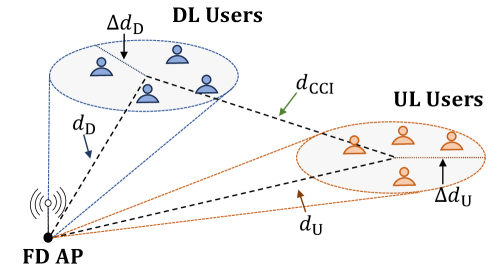
Figure 3: The considered FD MU-MIMO wireless networks in simulations.

In simulations, we set $\epsilon_{{\bf u}}=\epsilon_{{\bf v}}=\epsilon_{{\bf f}}=10^{-2}$ and $t_{\sf max}=n_{\sf max}=30$. We assume that the digital SIC can reduce the residual SI power after analog SIC down to the noise floor, i.e., $P_{\sf D}\kappa_{\sf a}\kappa_{\sf d}=\sigma_{\sf NF}^{2}$ as shown in Fig. 2. We also compare the HD system. For the HD system, we set $\kappa_{\sf a}=\kappa_{\sf d}=0$ and $\rho_{\sf CCI}=0$ in the considered FD system, and thus, we compute the sum of HD DL and UL spectral efficiencies as $\sum_{k=1}^{K_{\sf D}}R^{\sf HD}_{{\sf D},k}=(1-\lambda)\sum_{k=1}^{K_{\sf D}}R_{{\sf D},k}({\bf W})$ and $\sum_{k=1}^{K_{\sf U}}R^{\sf HD}_{{\sf U},k}=\lambda\sum_{k=1}^{K_{\sf U}}R_{{\sf U},k}({\bf W},{\bf F})$ without SI and CCI. We use $\lambda=1/2$. Then, we consider the following FD and HD benchmarks:

• (FD) qMM-qMMSE: The FD optimization algorithm which designed by modifying the MM precoding in [16] to incorporate quantization errors and adopting qMMSE.

• (FD) qRZF-qMMSE: The linear FD algorithm using by a quantization-aware RZF (qRZF) for precoding and qMMSE for combining.

• (HD) qGPI $\&$ qMMSE: The HD algorithm that uses a quantization-aware GPI (qGPI) based on the power method in [41] for precoding and qMMSE for combining.

• (HD) qWMMSE $\&$ qMMSE: The HD method that uses a quantization-aware weighted MMSE (qWMMSE) based approach [42] for precoding and qMMSE for combining.

• (HD) qWMMSE-AO $\&$ qMMSE: The HD approach that uses a qWMMSE alternating optimization (qWMMSE-AO) scheme inspired by successive convex approximation in [43] for precoding and qMMSE for combining.

• (HD) qRZF $\&$ qMMSE: The HD method that uses the qRZF for precoding and qMMSE for combining.

V-B Spectral Efficiency Analysis

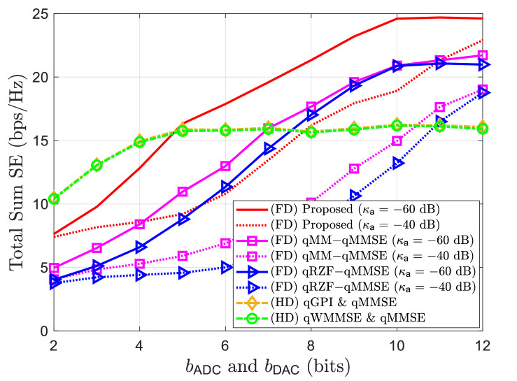
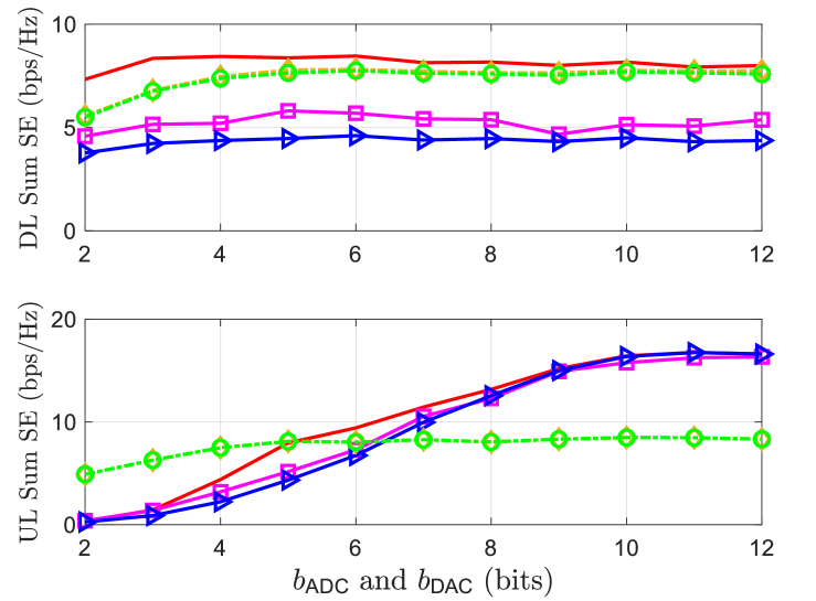
Figure 4: (a) The total sum SE with analog SIC capability $\kappa_{\sf a}\in\{-40,-60\}\,\mathrm{dB}$, (b) DL and UL sum SEs with $\kappa_{\sf a}=-60\,\mathrm{dB}$ versus the number of ADC and DAC bits for $N_{t}=N_{r}=16$, $K_{\sf D}=K_{\sf U}=4$, $P_{\sf D}=24\,\mathrm{dBm}$, $P_{\sf U}=23\,\mathrm{dBm}$.

Now, we compare the proposed method and other baselines in terms of the SE performance. Considering a small cell scenario, we set $P_{\sf D}=24\,\mathrm{dBm}$, $P_{\sf U}=23\,\mathrm{dBm}$, and $\kappa_{\sf a}=-60\,\mathrm{dB}$ which is typically considered to be a maximum analog SIC capability [37]. For the considered values, the condition in Proposition 1 for the required number of ADC bits is $b_{\sf ADC}>5.87$. Accordingly, we set $b_{{\sf ADC},n}=b_{{\sf DAC},m}=7$ bits $\forall n,m$ to have 1-bit margin, unless mentioned otherwise. The simulations are based on the considered AQNM model.

Fig. 4 illustrates that the total FD sum SE versus the resolution bits $b_{\sf ADC}$ and $b_{\sf DAC}$. We observe that the proposed method outperforms the benchmark FD methods. In the case of $\kappa_{\sf a}=-60\,\mathrm{dB}$, the proposed algorithm begins to provide the noticeable improvement than the HD cases when employing $b_{\sf ADC}=b_{\sf DAC}\geq 6$ bits. As shown in Fig. 4, the primary reason is that the UL sum SE is highly degraded compared to the HD case under $6$ bits due to the impact of the residual analog SI to the quantization noise – different from the well-known results in the HD system that using 4-bit ADC is sufficient [21, 22, 23, 24]. This result is analogous to the discussion in Remark 3. It is also noticeable that even more bits $b_{\sf ADC}=b_{\sf DAC}\geq 8$ are needed when $\kappa_{\sf a}=-40$ dB. Accordingly, it is necessary to improve the analog SIC capability as much as possible under coarse quantization. In addition, we note that the benchmark FD algorithms require more bits, i.e., $b_{\sf ADC}\geq 8$ with $\kappa_{\sf a}=-60$ dB, than the proposed method because of insufficient control over SI and IUI. Therefore, this reveals that careful optimization of the beamforming can reduce the required number of ADC bits, thereby offering more opportunities for enhancing the EE.

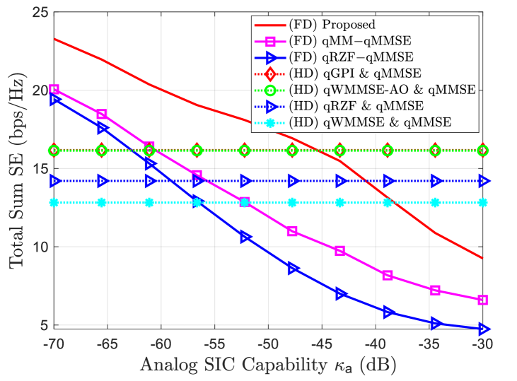
Figure 5: The total sum SE versus the analog SIC capability for $N_{t}=N_{r}=16$, $K_{\sf D}=K_{\sf U}=4$, $P_{\sf D}=24\,\mathrm{dBm}$, $P_{\sf U}=23\,\mathrm{dBm}$, and $b_{{\sf ADC},n}=b_{{\sf DAC},m}=7$ bits.

Fig. 5 shows the total sum SE versus the analog SIC capability. We can observe that worsening the analog SIC capability leads to the diminution of the total sum SE of all FD algorithms. With $7$ bits, the proposed method can achieve a noticeable SE gain compared to the HD systems when the analog SIC capability is $\kappa_{\sf a}<-50$ dB. This observation implies that the analog SIC capability has a significant impact on the FD systems as it directly determines the quantization noise power, which is a different result from the FD systems without quantization errors. In this respect, we can conjecture similar insight as in Fig. 4 that it is necessary to improve the beamforming design and the analog SIC capability to utilize lower-resolution ADCs.

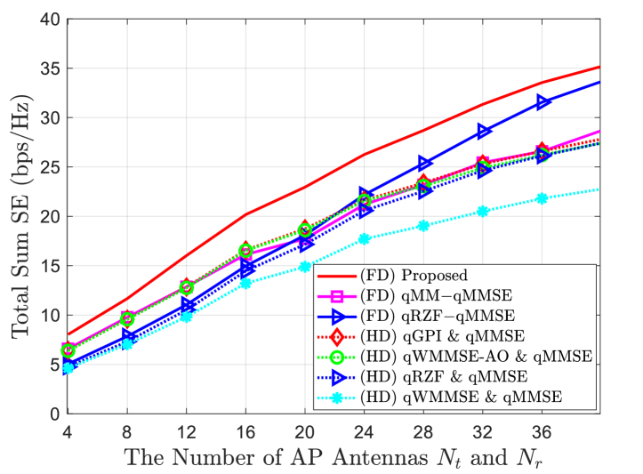
Figure 6: The total sum SE versus the number of AP antennas for $K_{\sf D}=K_{\sf U}=4$, $P_{\sf D}=24\,\mathrm{dBm}$, $P_{\sf U}=23\,\mathrm{dBm}$, $\kappa_{\sf a}=-60\,\mathrm{dB}$, and $b_{{\sf ADC},n}=b_{{\sf DAC},m}=7$ bits.

Fig. 6 demonstrates that the total sum SE versus the number of AP’s transmit and receive antennas. It is shown that the proposed algorithm accomplishes the highest sum SE over the FD and HD benchmarks. Moreover, as the number of antennas increases, the FD systems exhibit more improvement than the HD systems. Based on this observation, we can conjecture that the MIMO precoding with a larger number of antennas contributes to improving the sum SE by not only increasing the DL SINR but also decreasing the SI. This results suggest that it is more important to have larger antenna arrays with an optimized SI-aware beamformer in the quantized FD systems than the quantized HD systems.

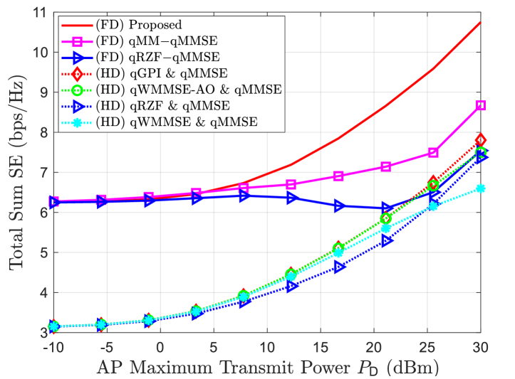
Figure 7: The total sum SE versus the AP transmit power for $N_{t}=N_{r}=4$, $K_{\sf D}=K_{\sf U}=2$, $P_{\sf U}=23\,\mathrm{dBm}$, $\kappa_{\sf a}=-60\,\mathrm{dB}$, and $b_{{\sf ADC},n}=b_{{\sf DAC},m}=7$ bits.

In Fig. 7, we evaluate the total sum SE versus the AP maximum transmit power. The proposed algorithm exhibits the highest SE. We note that the SE gain of the FD systems over the HD systems decreases with the AP transmit power for the FD benchmarks. This is because increasing the AP transmit power increases the SI, and it leads to the larger residual analog SI after analog SIC, which contributes to increasing the ADC quantization error. The proposed method, however, maintains the gain by managing the SI as well as the DL SINR. Consequently, optimizing precoding for SI reduction with DL SINR maximization is highly desirable in the quantized FD systems to efficiently utilize higher transmit power.

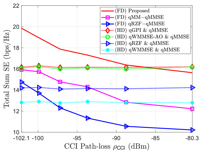
Figure 8: The total sum SE versus the CCI path-loss determined by $d_{\sf CCI}\in\{30,25,20,15,10,5\}\,\mathrm{m}$ for $N_{t}=N_{r}=16$, $K_{\sf D}=K_{\sf U}=4$, $P_{\sf D}=24\,\mathrm{dBm}$, $P_{\sf U}=23\,\mathrm{dBm}$, $\kappa_{\sf a}=-60\,\mathrm{dB}$, and $b_{{\sf ADC},n}=b_{{\sf DAC},m}=7$ bits.

In Fig. 8, we validate the total sum SE versus the CCI power by varying $d_{\sf CCI}$ from 30$\,\mathrm{m}$ to 5$\,\mathrm{m}$. Fig. 8 shows that the proposed algorithm achieves the highest performance when the CCI is lower than approximately $-88\,\mathrm{dBm}$. We note that all FD algorithms exhibit a gradual decrease in the total sum SE as the CCI increases or equivalently, $d_{\sf CCI}$ decreases, thereby detrimentally affecting the DL sum SE. Therefore, it is critical for FD systems to serve DL and UL user groups that are properly separated in distance through careful scheduling.

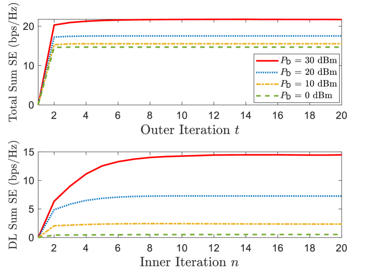
Figure 9: The convergence of the outer and inner iterations for $N_{t}=N_{r}=16$, $K_{\sf D}=K_{\sf U}=4$, $P_{\sf U}=23\,\mathrm{dBm}$, $\kappa_{\sf a}=-60\,\mathrm{dB}$, and $b_{{\sf ADC},n}=b_{{\sf DAC},m}=7$ bits.

Fig. 9 illustrates the numerical convergence of the proposed algorithm. As $P_{\sf D}$ improves, it requires a greater number of inner iterations for the algorithm to converge, while the number of outer iterations remains almost unchanged. Specifically, the highest number of the inner iteration converges within approximately 10 iterations, and that of the outer iteration is 2 iterations. Since it can be operated with a small number of iterations, the proposed algorithm is practical and computationally beneficial for the wireless communications.

V-C Energy Efficiency Analysis

Now, we evaluate the EE performance of proposed algorithm to examine the desirable range of the quantization resolution that provides the highest EE while guaranteeing the SE advantage of FD systems over HD systems. According to [21], we define the normalized EE using (29) and (30) as

$$\mathrm{EE}=\frac{\sum_{k=1}^{K_{\sf D}}R_{{\sf D},k}({\bf W})+\sum_{k=1}^{K_{\sf U}}R_{{\sf U},k}({\bf W};{\bf F})}{P_{\sf AP}+P_{\sf UE}},$$ (66)

where the unit of EE is $\mathrm{bits/Joule/Hz}$, $P_{\sf AP}$ is total power consumption of the AP, and $P_{\sf UE}$ is a sum of total power consumption of DL and UL users.

Then, based on [44, 45], we define $P_{\sf AP}$ as

$$P_{\sf AP}=P^{\sf tx}_{\sf AP}+P^{\sf rx}_{\sf AP},$$ (67)

where $P^{\sf tx}_{\sf AP}=P_{\sf LO}+N_{t}(2P_{\sf LP}+2P_{\sf M}+P_{\sf H}+\kappa^{-1}_{\sf PA}P_{\sf TX})+2N_{t}(P_{\sf AGC}+P_{\sf DAC}(b_{\sf DAC},f_{s}))+P_{\sf BB}$ and $P^{\sf rx}_{\sf AP}=P_{\sf LO}+N_{r}(2P_{\sf LP}+2P_{\sf M}+P_{\sf H}+P_{\sf LNA})+2N_{r}(P_{\sf AGC}+P_{\sf ADC}(b_{\sf ADC},f_{r}))+P_{\sf BB}.$ Here, $P^{\sf tx}_{\sf AP}$ and $P^{\sf rx}_{\sf AP}$ are a transmit and receive power consumption at the AP, respectively. In addition, $\kappa_{\sf PA}$ is the power amplifier efficiency, and $P_{\sf TX}$, $P_{\sf LO}$, $P_{\sf LP}$, $P_{\sf M}$, $P_{\sf H}$, $P_{\sf DAC}$, $P_{\sf ADC}$, $P_{\sf LNA}$, $P_{\sf AGC}$, and $P_{\sf BB}$ are the power consumptions of a target transmit power, a local oscillator, a low-pass filter, a mixer, a $90^{\circ}$ hybrid with buffer, DAC, ADC, a low noise amplifier, an automatic gain control, and a baseband processor, respectively [21, 44]. Since we use maximum transmit power, we have $P_{\sf TX}=P_{\sf D}$, and $P_{\sf DAC}$ and $P_{\sf ADC}$ (in $\mathrm{W}$) are given as [44, 46]

$$P_{\sf DAC} =1.5\times 10^{-5}\cdot 2^{b_{\sf DAC}}+9\times 10^{-12}\cdot f_{s}\cdot b_{\sf DAC},$$ (68)

$$P_{\sf ADC} =c_{e}\cdot f_{r}\cdot 2^{b_{\sf ADC}},$$ (69)

where $c_{e}$ is an power consumption per conversion step, and $f_{s}$ and $f_{r}$ are sampling rates of AP’s transmitter and receiver, respectively. We use $c_{e}=494\;\mathrm{fJ}$ in [47], and $f_{s}=f_{r}=500$ MHz which is critically sampled.

Now, based on [44, 45], we can represent $P_{\sf UE}$ as

$$P_{\sf UE}=K_{\sf D}P^{\sf DL}_{\sf UE}+K_{\sf U}P^{\sf UL}_{\sf UE},$$ (70)

where the total power consumption of DL and UL users are

$$P^{\sf DL}_{\sf UE}= \,P_{\sf LO}\!+\!2P_{\sf LP}\!+\!2P_{\sf M}\!+\!P_{\sf H}\!+\!P^{\sf UE}_{\sf LNA}\!+\!2P_{\sf AGC}\!+\!P_{\sf BB},$$ (71)

$$P^{\sf UL}_{\sf UE}= \,P_{\sf LO}\!+\!2P_{\sf LP}\!+\!2P_{\sf M}\!+\!P_{\sf H}\!+\!P^{\sf UE}_{\sf PA}\!+\!2P_{\sf AGC}\!+\!P_{\sf BB}.$$ (72)

We assume that the parameters (e.g., $P_{\sf LO}$, $P_{\sf LP}$, $P_{\sf M}$, $P_{\sf H}$, $P_{\sf AGC}$, and $P_{\sf BB}$) used to define the total power consumption for the AP are the same as (71) and (72). $P^{\sf UE}_{\sf LNA}$ and $P^{\sf UE}_{\sf PA}=\kappa_{\sf PA}^{-1}P_{\sf U}$ are a power consumption of the low noise amplifier at the DL user and the power amplifier at the UL user, respectively. We set the circuit power consumption according to [21, 44, 48].

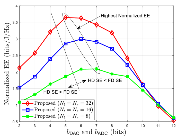
Figure 10: The normalized EE versus the ADC and DAC bits for $N_{t}=N_{r}\in\{8,16,32\}$, $K_{\sf D}=K_{\sf U}=4$, $P_{\sf D}=24\,\mathrm{dBm}$, $P_{\sf U}=23\,\mathrm{dBm}$, $\kappa_{\sf a}=-60\,\mathrm{dB}$.

In Fig. 10, we evaluate the EE with respect to the number of ADC and DAC bits. The left region, divided by the black line, represents the area where the total sum SE of the proposed algorithm is lower than that of the HD system, while the right region denotes the area where the total sum SE of the proposed algorithm exceeds that of the HD system. The key finding is that the EE of the FD system improves as reducing the ADC and DAC resolutions, and there exists the optimal number of bits which is around $6$ bits. Since we observed from both the analysis in Section III and numerical results in Section V-B that at least $b_{\sf ADC}\geq 6$ is required for the consider system, it seems desirable to design the quantized FD MU-MIMO system with 6 to 8 bits in terms of both the SE and EE.

Overall, our study shows that $b_{\sf ADC}\geq 6$ is needed even for the ADC-favorable scenario, i.e., high analog SIC capability and moderate transmit power. In addition, the adopted quantization model is less restrictive in reducing the ADC resolution than the practical ADC operation. Therefore, it is concluded that the minimum required ADC bits for the considered FD system is around $6$ bits in order to simultaneously achieve the high SE and the high EE. Other important findings include that increasing the number of antennas with SI-aware beamforming can reduce the required number of bits by mitigating the SI, analog SIC capability is a primary performance factor for the quantized FD MIMO systems, and DL and UL users need to be properly scheduled to guarantee minimal CCI.

VI Conclusion

In this paper, we provide a comprehensive characterization of the quantized FD MU-MIMO system design, specifically focusing on the challenges posed by employing low-resolution ADCs. In contrast to prior research, our approach accounts for the influence of analog SIC on ADC quantization. Our investigation led to the derivation of the requisite number of ADC bits to prevent the submersion of desired UL signals in quantization noise and guarantee ADC resolvability, pivotal factors in determining ADC resolution for the system. The analysis underscores the significance of managing residual analog SI in quantized FD systems. Inspired by the findings, we introduce an advanced SI-aware beamforming design, which, by identifying optimal stationary points for the precoder, demonstrates superior performance. Numerical analyses further illuminate that the proposed SI-aware beamforming reduces the required number of ADC bits compared to FD benchmarks, thereby providing more opportunities for enhancing EE. Diverging from HD systems, our study uncovered that a minimum of 6 ADC bits is essential for practical FD scenarios. In particular, employing 6 to 8-bit ADCs shows FD systems outperforming HD systems without compromising UL SE when using the proposed method, concurrently attaining high EE. Therefore, it is concluded that FD systems need to employ more ADC bits than the HD system, i.e., minimum $6$ bits, which can be achieved by the proposed method, surpassing the performance of HD systems and optimizing EE.

Appendix A Proof of Lemma 1

We note that the power constraint in (58) can be ignored indeed since $\gamma_{{\sf D},k}(\bar{\bf v})$ and $\gamma_{{\sf U},k}(\bar{\bf v};{\bf F})$ are invariant up to the scaling of $\bar{\bf v}$. Then, the Lagrangian function of the problem is

$$\mbox{$\mathcal{L}$}(\bar{{\bf v}})=\mathrm{log}_{2}\prod_{k=1}^{K_{\sf D}}\left(\frac{\bar{{\bf v}}^{\sf H}{\bf A}_{k}\bar{{\bf v}}}{\bar{{\bf v}}^{\sf H}{\bf B}_{k}\bar{{\bf v}}}\right)\prod_{k=1}^{K_{\sf U}}\left(\frac{\bar{{\bf v}}^{\sf H}{\bf C}_{k}\bar{{\bf v}}}{\bar{{\bf v}}^{\sf H}{\bf D}_{k}\bar{{\bf v}}}\right).$$ (73)

We need to compute the derivative of (73) to obtain the first-order optimality condition. Let us define $\lambda(\bar{{\bf v}})$ as

$$\lambda(\bar{{\bf v}})= \;\prod_{k=1}^{K_{\sf D}}\left(\frac{\bar{{\bf v}}^{\sf H}{\bf A}_{k}\bar{{\bf v}}}{\bar{{\bf v}}^{\sf H}{\bf B}_{k}\bar{{\bf v}}}\right)\prod_{k=1}^{K_{\sf U}}\left(\frac{\bar{{\bf v}}^{\sf H}{\bf C}_{k}\bar{{\bf v}}}{\bar{{\bf v}}^{\sf H}{\bf D}_{k}\bar{{\bf v}}}\right),$$ (74)

and thus $\mbox{$\mathcal{L}$}(\bar{{\bf v}})=\mathrm{log_{2}}\,\lambda(\bar{{\bf v}})$.

Now, we compute a derivative of $\mbox{$\mathcal{L}$}(\bar{{\bf v}})$ which is denoted as

$$\frac{\partial\mbox{$\mathcal{L}$}(\bar{{\bf v}})}{\partial\bar{{\bf v}}^{\sf H}}=\frac{1}{\lambda(\bar{{\bf v}})\mathrm{ln}\,2}\frac{\partial\lambda(\bar{{\bf v}})}{\partial\bar{{\bf v}}^{\sf H}}.$$ (75)

Hence, the derivative of $\lambda(\bar{{\bf v}})$ is computed as

$$\frac{\partial\lambda(\bar{{\bf v}})}{\partial\bar{{\bf v}}^{\sf H}}=$$ (76)

$$2\lambda(\bar{{\bf v}})\left(\sum_{k=1}^{K_{\sf D}}\left(\frac{{\bf A}_{k}\bar{{\bf v}}}{\bar{{\bf v}}^{\sf H}{\bf A}_{k}\bar{{\bf v}}}-\frac{{\bf B}_{k}\bar{{\bf v}}}{\bar{{\bf v}}^{\sf H}{\bf B}_{k}\bar{{\bf v}}}\right)+\sum_{k=1}^{K_{\sf U}}\left(\frac{{\bf C}_{k}\bar{{\bf v}}}{\bar{{\bf v}}^{\sf H}{\bf C}_{k}\bar{{\bf v}}}-\frac{{\bf D}_{k}\bar{{\bf v}}}{\bar{{\bf v}}^{\sf H}{\bf D}_{k}\bar{{\bf v}}}\right)\right).$$

Setting (76) equal to zero with reorganization provides the stationary condition as

$$\lambda_{\sf num}(\bar{{\bf v}})\left(\sum_{k=1}^{K_{\sf D}}\frac{{\bf A}_{k}}{\bar{{\bf v}}^{\sf H}{\bf A}_{k}\bar{{\bf v}}}+\sum_{k=1}^{K_{\sf U}}\frac{{\bf C}_{k}}{\bar{{\bf v}}^{\sf H}{\bf C}_{k}\bar{{\bf v}}}\right)\bar{{\bf v}}$$

$$=\lambda(\bar{{\bf v}})\lambda_{\sf den}(\bar{{\bf v}})\left(\sum_{k=1}^{K_{\sf D}}\frac{{\bf B}_{k}}{\bar{{\bf v}}^{\sf H}{\bf B}_{k}\bar{{\bf v}}}+\sum_{k=1}^{K_{\sf U}}\frac{{\bf D}_{k}}{\bar{{\bf v}}^{\sf H}{\bf D}_{k}\bar{{\bf v}}}\right)\bar{{\bf v}}.$$ (77)

Accordingly, we derive the necessary condition of the first-order optimality condition from (A) as

$${\bf A}_{\sf KKT}(\bar{{\bf v}})\bar{{\bf v}}=\lambda(\bar{{\bf v}}){\bf B}_{\sf KKT}(\bar{{\bf v}})\bar{{\bf v}},$$ (78)

where ${\bf A}_{\sf KKT}(\bar{{\bf v}})$ and ${\bf B}_{\sf KKT}(\bar{{\bf v}})$ are defined in (60) and (61), respectively. This completes the proof. ∎

References

• [1] S. Yoo, S. Park, and J. Choi, “Joint Precoding and Combining for Quantized Full-Duplex MU-MIMO Systems,” in IEEE Veh. Technol. Conf. Workshop (VTC), 2023, pp. 1–6.
• [2] Z. Zhang, Y. Xiao, Z. Ma, M. Xiao, Z. Ding, X. Lei, G. K. Karagiannidis, and P. Fan, “6G Wireless Networks: Vision, Requirements, Architecture, and Key Technologies,” IEEE Veh. Technol. Mag., vol. 14, no. 3, pp. 28–41, 2019.
• [3] M. Z. Chowdhury, M. Shahjalal, S. Ahmed, and Y. M. Jang, “6G Wireless Communication Systems: Applications, Requirements, Technologies, Challenges, and Research Directions,” IEEE Open J. Commun. Soc., vol. 1, pp. 957–975, 2020.
• [4] S. Elmeadawy and R. M. Shubair, “6G Wireless Communications: Future Technologies and Research Challenges,” in Proc. Int. Conf. Electr. Comput. Technol. Appl. (ICECTA).   IEEE, 2019, pp. 1–5.
• [5] R. Li, Y. Chen, G. Y. Li, and G. Liu, “Full-Duplex Cellular Networks,” IEEE Commun. Mag., vol. 55, no. 4, pp. 184–191, 2017.
• [6] S. Jacobsson, G. Durisi, M. Coldrey, T. Goldstein, and C. Studer, “Quantized Precoding for Massive MU-MIMO,” IEEE Trans. Commun., vol. 65, no. 11, pp. 4670–4684, 2017.
• [7] S. Chen, M. Beach, and J. McGeehan, “Division-Free Duplex for Wireless Applications,” Electronics Lett., vol. 34, no. 2, pp. 147–148, 1998.
• [8] T. Riihonen, S. Werner, and R. Wichman, “Mitigation of Loopback Self-Interference in Full-Duplex MIMO Relays,” IEEE Trans. Signal Process., vol. 59, no. 12, pp. 5983–5993, 2011.
• [9] M. Duarte, C. Dick, and A. Sabharwal, “Experiment-Driven Characterization of Full-Duplex Wireless Systems,” IEEE Trans. Wireless Commun., vol. 11, no. 12, pp. 4296–4307, 2012.
• [10] D. Bharadia, E. McMilin, and S. Katti, “Full Duplex Radios,” in Proc. ACM SIGCOMM Conf. 2013, 2013, pp. 375–386.
• [11] H. A. Suraweera, I. Krikidis, G. Zheng, C. Yuen, and P. J. Smith, “Low-Complexity End-to-End Performance Optimization in MIMO Full-Duplex Relay Systems,” IEEE Trans. Wireless Commun., vol. 13, no. 2, pp. 913–927, 2014.
• [12] A. Almradi, P. Xiao, and K. A. Hamdi, “Hop-by-Hop ZF Beamforming for MIMO Full-Duplex Relaying With Co-Channel Interference,” IEEE Trans. Commun., vol. 66, no. 12, pp. 6135–6149, 2018.
• [13] Y. Shao and T. A. Gulliver, “Precoding Design for Two-Way MIMO Full-Duplex Amplify-and-Forward Relay Communication Systems,” IEEE Access, vol. 7, pp. 76 458–76 469, 2019.
• [14] D. Nguyen, L.-N. Tran, P. Pirinen, and M. Latva-aho, “On the Spectral Efficiency of Full-Duplex Small Cell Wireless Systems,” IEEE Trans. Wireless Commun., vol. 13, no. 9, pp. 4896–4910, 2014.
• [15] S. Huberman and T. Le-Ngoc, “MIMO Full-Duplex Precoding: A Joint Beamforming and Self-Interference Cancellation Structure,” IEEE Trans. Wireless Commun., vol. 14, no. 4, pp. 2205–2217, 2014.
• [16] J. Kim, W. Choi, and H. Park, “Beamforming for Full-Duplex Multiuser MIMO Systems,” IEEE Trans. Veh. Technol., vol. 66, no. 3, pp. 2423–2432, 2016.
• [17] A. C. Cirik, “Fairness Considerations for Full Duplex Multi-User MIMO Systems,” IEEE Wireless Commun. Lett., vol. 4, no. 4, pp. 361–364, 2015.
• [18] C. Risi, D. Persson, and E. G. Larsson, “Massive MIMO with 1-bit ADC,” arXiv preprint arXiv:1404.7736, 2014.
• [19] N. Liang and W. Zhang, “Mixed-ADC Massive MIMO,” IEEE J. Sel. Areas Commun., vol. 34, no. 4, pp. 983–997, 2016.
• [20] J. Choi, B. L. Evans, and A. Gatherer, “Resolution-Adaptive Hybrid MIMO Architectures for Millimeter Wave Communications,” IEEE Trans. Signal Process., vol. 65, no. 23, pp. 6201–6216, 2017.
• [21] J. Choi, J. Park, and N. Lee, “Energy Efficiency Maximization Precoding for Quantized Massive MIMO Systems,” IEEE Trans. Wireless Commun., vol. 21, no. 9, pp. 6803–6817, 2022.
• [22] C. Studer and G. Durisi, “Quantized Massive MU-MIMO-OFDM Uplink,” IEEE Trans. on Commun., vol. 64, no. 6, pp. 2387–2399, 2016.
• [23] D. Verenzuela, E. Björnson, and M. Matthaiou, “Hardware Design and Optimal ADC Resolution for Uplink Massive MIMO Systems,” in IEEE Sensor Array and Multichannel Signal Process. Workshop, 2016, pp. 1–5.
• [24] S. Jacobsson, G. Durisi, M. Coldrey, U. Gustavsson, and C. Studer, “Throughput Analysis of Massive MIMO Uplink With Low-Resolution ADCs,” IEEE Trans. on Wireless Commun., vol. 16, no. 6, pp. 4038–4051, 2017.
• [25] J. Dai, Y. Wang, C. Pan, K. Zhi, H. Ren, and K. Wang, “Reconfigurable Intelligent Surface Aided Massive MIMO Systems With Low-Resolution DACs,” IEEE Commun. Lett., vol. 25, no. 9, pp. 3124–3128, 2021.
• [26] X. Hu, C. Zhong, X. Chen, W. Xu, H. Lin, and Z. Zhang, “Cell-Free Massive MIMO Systems With Low Resolution ADCs,” IEEE Trans. Commun., vol. 67, no. 10, pp. 6844–6857, 2019.
• [27] S. Kim, J. Choi, and J. Park, “Downlink NOMA for Short-Packet Internet of Things Communications With Low-Resolution ADCs,” IEEE Int. Things J., vol. 10, no. 7, pp. 6126–6139, 2022.
• [28] S. Park, J. Choi, J. Park, W. Shin, and B. Clerckx, “Rate-Splitting Multiple Access for Quantized Multiuser MIMO Communications,” IEEE Trans. Wireless Commun., 2023.
• [29] J. Dai, J. Liu, J. Wang, J. Zhao, C. Cheng, and J.-Y. Wang, “Achievable Rates for Full-Duplex Massive MIMO Systems With Low-Resolution ADCs/DACs,” IEEE Access, vol. 7, pp. 24 343–24 353, 2019.
• [30] C. Kong, C. Zhong, S. Jin, S. Yang, H. Lin, and Z. Zhang, “Full-Duplex Massive MIMO Relaying Systems With Low-Resolution ADCs,” IEEE Trans. Wireless Commun., vol. 16, no. 8, pp. 5033–5047, 2017.
• [31] P. Anokye, R. K. Ahiadormey, and K.-J. Lee, “Full-Duplex Cell-Free Massive MIMO With Low-Resolution ADCs,” IEEE Trans. on Veh. Technol., vol. 70, no. 11, pp. 12 179–12 184, 2021.
• [32] Q. Ding, Y. Lian, and Y. Jing, “Performance Analysis of Full-Duplex Massive MIMO Systems With Low-Resolution ADCs/DACs Over Rician Fading Channels,” IEEE Trans. Veh. Technol., vol. 69, no. 7, pp. 7389–7403, 2020.
• [33] T. Riihonen and R. Wichman, “Analog and Digital Self-interference Cancellation in Full-Duplex MIMO-OFDM Transceivers with Limited Resolution in A/D Conversion,” in IEEE Asilomar Conf. on Signals, Systems and Computers, 2012, pp. 45–49.
• [34] D. Korpi, T. Riihonen, V. Syrjälä, L. Anttila, M. Valkama, and R. Wichman, “Full-Duplex Transceiver System Calculations: Analysis of ADC and Linearity Challenges,” IEEE Trans. Wireless Commun., vol. 13, no. 7, pp. 3821–3836, 2014.
• [35] A. K. Fletcher, S. Rangan, V. K. Goyal, and K. Ramchandran, “Robust Predictive Quantization: Analysis and Design Via Convex Optimization,” IEEE J. Sel. Topics Signal Process., vol. 1, no. 4, pp. 618–632, 2007.
• [36] L. Fan, S. Jin, C.-K. Wen, and H. Zhang, “Uplink Achievable Rate for Massive MIMO Systems With Low-Resolution ADC,” IEEE Commun. Lett., vol. 19, no. 12, pp. 2186–2189, 2015.
• [37] J. Kim, H. Lee, H. Do, J. Choi, J. Park, W. Shin, Y. C. Eldar, and N. Lee, “On the Learning of Digital Self-Interference Cancellation in Full-Duplex Radios,” arXiv preprint arXiv:2308.05966, 2023.
• [38] R. H. Walden, “Analog-to-Digital Converter Survey and Analysis,” IEEE J. Sel. Areas Commun., vol. 17, no. 4, pp. 539–550, 1999.
• [39] S. Sun, T. S. Rappaport, S. Rangan, T. A. Thomas, A. Ghosh, I. Z. Kovacs, I. Rodriguez, O. Koymen, A. Partyka, and J. Jarvelainen, “Propagation Path Loss Models for 5G Urban Micro-and Macro-Cellular Scenarios,” in Proc. IEEE Veh. Technol. Conf., 2016, pp. 1–6.
• [40] A. Adhikary, J. Nam, J.-Y. Ahn, and G. Caire, “Joint Spatial Division and Multiplexing—The Large-Scale Array Regime,” IEEE Trans. Inf. Theory, vol. 59, no. 10, pp. 6441–6463, 2013.
• [41] J. Choi, N. Lee, S.-N. Hong, and G. Caire, “Joint User Selection, Power Allocation, and Precoding Design With Imperfect CSIT for Multi-Cell MU-MIMO Downlink Systems,” IEEE Trans. Wireless Commun., vol. 19, no. 1, pp. 162–176, 2019.
• [42] S. S. Christensen, R. Agarwal, E. De Carvalho, and J. M. Cioffi, “Weighted Sum-Rate Maximization using Weighted MMSE for MIMO-BC Beamforming Design,” IEEE Trans. Wireless Commun., vol. 7, no. 12, pp. 4792–4799, 2008.
• [43] M. Razaviyayn, “Successive Convex Approximation: Analysis and Applications,” Ph.D. dissertation, Univ. of Minnesota, Minneapolis, MN, 2014.
• [44] J. Zhang, L. Dai, Z. He, S. Jin, and X. Li, “Performance Analysis of Mixed-ADC Massive MIMO Systems Over Rician Fading Channels,” IEEE J. Sel. Areas Commun., vol. 35, no. 6, pp. 1327–1338, 2017.
• [45] J. Zhang, L. Dai, Z. He, B. Ai, and O. A. Dobre, “Mixed-ADC/DAC Multipair Massive MIMO Relaying Systems: Performance Analysis and Power Optimization,” IEEE Trans. Commun., vol. 67, no. 1, pp. 140–153, 2018.
• [46] Q. Ding, Y. Deng, and X. Gao, “Spectral and Energy Efficiency of Hybrid Precoding for mmWave Massive MIMO With Low-Resolution ADCs/DACs,” IEEE Access, vol. 7, pp. 186 529–186 537, 2019.
• [47] H.-S. Lee and C. G. Sodini, “Analog-to-Digital Converters: Digitizing the Analog World,” Proc. of the IEEE, vol. 96, no. 2, pp. 323–334, 2008.
• [48] Y. Shang, D. Cai, W. Fei, H. Yu, and J. Ren, “An 8mW Ultra Low Power 60GHz Direct-conversion Receiver with 55dB Gain and 4.9 dB Noise Figure in 65nm CMOS,” in IEEE Radio-Frequency Integration Technol., 2012, pp. 47–49.