Embedded Named Entity Recognition using Probing Classifiers

Abstract

Extracting semantic information from generated text is a useful tool for applications such as automated fact checking or retrieval augmented generation. Currently, this requires either separate models during inference, which increases computational cost, or destructive fine-tuning of the language model. Instead, we propose directly embedding information extraction capabilities into pre-trained language models using probing classifiers, enabling efficient simultaneous text generation and information extraction. For this, we introduce an approach called EMBER and show that it enables named entity recognition in decoder-only language models without fine-tuning them and while incurring minimal additional computational cost at inference time. Specifically, our experiments using GPT-2${}_{\text{XL}}$ show that EMBER maintains high token generation rates during streaming text generation, with only a negligible decrease in speed of around 1% compared to a 43.64% slowdown measured for a baseline using a separate NER model. Code and data are available at https://github.com/nicpopovic/EMBER.

Embedded Named Entity Recognition using Probing Classifiers

Nicholas Popovič  and Michael Färber Karlsruhe Institute of Technology (KIT), Germany {popovic, michael.faerber}@kit.edu

1 Introduction

Combining pre-trained language models (LMs) and external information at inference time is a widely used approach, for example as a means of improving the factual accuracy of generated texts in knowledge-intensive tasks Lewis et al. (2020); Guu et al. (2020); Gao et al. (2024). To effectively gather relevant information, there are generally two main strategies for extracting semantic data from the current context, each with its own drawbacks. The first strategy involves integrating the extraction process into text generation. This method, exemplified by research from Schick et al. (2023) and Zhang (2023), requires generating queries during the inference phase. Although this approach is direct, it has the downside of altering the LM through fine-tuning, which can lead to issues like catastrophic forgetting, as discussed by Goodfellow et al. (2015). The second strategy employs an external system for information extraction (IE). Studies by Shi et al. (2023), Ram et al. (2023), and Dhuliawala et al. (2023) illustrate this approach. While this method preserves the integrity of the LM, making it non-destructive, it demands substantial additional resources during inference, which can be a significant limitation for time-sensitive applications such as streaming text generation.

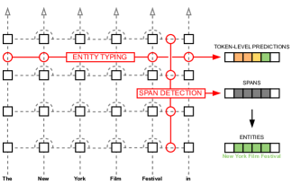
Figure 1: Illustration of the proposed approach for named entity recognition using probing classifiers. One classifier performs token-level entity typing using hidden states at a single layer, while a second classifier detects spans based on attention weights. Both predictions are aggregated into span-level entity predictions.

Meanwhile, research into the mechanistic interpretability of LMs has shown that substantial semantic information can be recovered from individual internal representations. A common diagnostic tool are simple classifiers, called probing classifiers Belinkov and Glass (2019), trained to perform specific tasks using a subset of the internal representations of a (frozen) LM as their feature space. While their validity as a means for understanding how and where information is stored in LMs is debated Cao et al. (2021); Belinkov (2022), probing classifiers have been shown able to map internal representations to syntactic and semantic information Raganato and Tiedemann (2018); Clark et al. (2019); Mareček and Rosa (2019); Htut et al. (2019); Pimentel et al. (2020); Schouten et al. (2022). While the majority of this research has been conducted using encoder LMs, studies have shown that similar information is recoverable from specific internal states of decoder-only LMs Meng et al. (2022); Geva et al. (2023); Hernandez et al. (2023); Ghandeharioun et al. (2024). We therefore explore whether, rather than as a diagnostic tool, probing classifiers can be used for non-destructive, light-weight, and continuous IE in decoder-only LMs at inference time.

In this work, we develop an approach we call Embedded Named Entity Recognition (EMBER) for performing named entity recognition (NER), a central IE subtask consisting of mention detection and entity typing, using only a LM’s internal representations as feature space without further finetuning thereof. As illustrated in figure 1, the process involves two probing classifiers: The first performs tokenwise type classification based on the hidden state at a single transformer sublayer, while the second detects spans based on the LMs attention weights between two tokens. Finally, the outputs of both are fused into span-level entity predictions.

We conduct a series of experiments using multiple LMs, NER datasets, and task settings to evaluate the performance of EMBER and the factors which influence it:

First, we examine a variety of combinations of internal representations in order to show which lead to the best results (4.1). We find that hidden states, especially at deeper layers, carry sufficient information to allow for entity typing with high F1 scores (approx. 92-96%, depending on the specific LM and dataset) and that the most accurate span detection can be achieved by classifying the attention weights directed at the first token of an entity from the first token following the span.

Next, we evaluate our approach on two common NER benchmarks in a supervised learning setting (4.2). Here we find that EMBER achieves F1 scores of up to 80-85% while requiring substantially fewer additional parameters than state-of-the-art finetuned approaches based on encoder LMs (<1% relative to LM size). When compared to in-context learning, i.e. the prevalent method of using decoder-only LMs without finetuning, we find that our approach performs significantly better in the supervised setting since it is able to make use of the full extent of training data, rather than being limited by the LMs context length. Results collected across 7 LMs ranging from 125m to 6.9b parameters in size (4.3) suggest that while higher F1 scores can be expected for larger models, entity typing performance is dictated by the hidden representation’s size rather than the overall amount model parameters and that, similarly, mention detection accuracy depends mainly on the number of attention heads, rather than the total model size.

Following supervised learning, we perform experiments in few-shot learning (4.4). We show that while in 1-shot and 5-shot scenarios, our approach is outperformed by in-context learning in terms of F1 scores, it proves useful in data constrained settings where the amount of annotated data available is insufficient for supervised learning but too large to fit into in-context demonstrations (>20-shot).

Finally, we use EMBER for NER during streaming text generation (5) to show the efficiency of the approach. We find that in order to achieve adequate performance on generated text, probing classifiers need to be trained on generated texts annotated by an auxiliary NER model. Our approach requires additional parameters amounting to less than 1% of the LM’s parameters and we show that due to its ability to operate incrementally, EMBER has a minimal impact on token generation rates. Specifically, we measure only around 1% slowdown during streaming text generation, where a baseline model causes a 43.64% slowdown.

In conclusion, we make the following contributions: We propose EMBER, a light-weight approach for adding NER capabilities to decoder-only LMs without finetuning. We show that our approach can achieve F1 scores of 80-85% while involving minimal additional computational overhead and can easily integrate substantially larger amounts of training data than in-context learning. We provide insight into which architecture parameters of decoder-LMs determine how well our approach will work. Lastly, we showcase efficient simultaneous text generation and NER, a novel usecase enabled by our approach.

2 Task Description

NER consists of two subtasks, namely mention detection and entity typing. Given a text as a sequence of tokens $t_{1},...t_{N}$, and a set of entity types $E$, mention detection involves locating all spans $t_{i},...t_{j}$, where $1<i,j<N$, corresponding to mentions of entities within the text. Entity typing is the task of assigning the correct entity type $e\in E$ to each mention. For Transformer-based approaches, NER is typically framed as a token classification task, where each token $t_{i}$ is assigned a label $y_{i}$ based on whether it is the first token of a mention (B), inside a mention (I) or outside of a mention (O).

3 EMBER

In this section we introduce our approach for building a NER system based on probing internal representations of pretrained, decoder-only LMs. Given a model $M$ with $L$ layers, a hidden state $h_{i}^{l}$ is the output at a single transformer sublayer, where $l\in[1,...,L]$ is the index of the sublayer and $i$ is the index of the input token. The attention weights between two tokens are denoted as $A_{j,i}$, where $j\geq i$ due to autoregressivity. Our approach entails two key steps, namely tokenwise entity type classification based on $h_{i}^{l}$ (3.1) and span detection based on $A_{j,i}$(3.2), the results of which are then combined to form a complete NER pipeline using a mechanism we call label propagation (3.3).

3.1 Tokenwise Classification

Prior work has shown that individual hidden states contain sufficent information to recover semantic information about entities, suggesting that these may represent a suitable feature space for our goal of entity typing. We therefore perform tokenwise classification by learning $f_{type}$ such that:

$$f_{type}(h_{i}^{l})=\hat{y}_{i},$$ (1)

where $\hat{y}_{i}$ is a prediction in IOB2 format.

However, the autoregressive nature of decoder-only LMs results in two inherent issues we will address in the following. (1) Firstly, entities which have their type modified by context following the mention cannot be correctly classified (For example, in the phrase "Harry Potter is a book title.", "Harry Potter" may be classified as a person given only the initial two words, while the remaining context makes the assignment of a type such as "work of art" more suitable. See D for an illustration of this example.). While, this issue is an inherent limitation of EMBER, our experiments show that its impact on general NER performance is limited. (2) The second issue arises for entities spanning multiple tokens. Consider the composite phrase "New York Film Festival" (see also figure 1 and appendix D), which, given the annotation schema for Ontonotes5 Hovy et al. (2006), should be assigned the entity type "EVENT". Given only the partial phrase "New York", however, the most appropriate entity type to assign is "GPE". We therefore expect that a token-level classifier outlined above will not predict all tokens in this phrase as belonging to the class "EVENT". More generally, classifying on a per-token basis does not guarantee that the same class is assigned to all tokens within a mention span. In the following section, we therefore provide a method for detecting entity spans, using which we can then aggregate tokenwise predictions to span-level predictions.

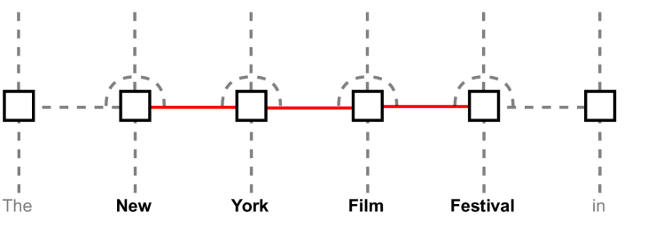
(a) adjacency classification

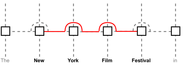
(b) span classification $j=k$

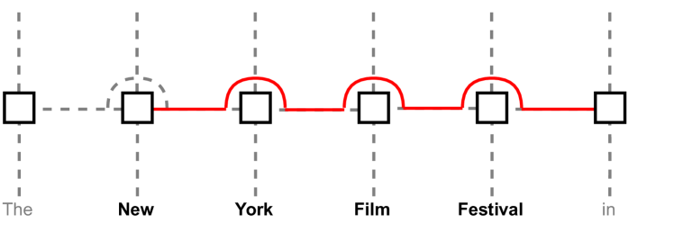
(c) span classification $j=k-1$

Figure 2: Illustration of the different span detection methods. Red colors indicate which attention weights to classify as positive for the example span "New York Film Festival". Attention weights are only shown for a single layer, but are generally used at all layers.

3.2 Span Detection

Since attention is the mechanism by which decoder-only LMs incorporate information from preceeding tokens, we hypothesize that $A_{j,i}$ contains different information based on whether or not $M$ represents $t_{i}$ and $t_{j}$ as tokens within the same span. Below, we propose two different approaches for identifying spans based on $A_{j,i}$:

Adjacency Classification. In adjacency classification, illustrated in figure 2 (a), we train a classifier to predict whether two adjacent tokens belong to the same mention ($a_{i,j}=1$ if so, $a_{i,j}=0$ otherwise), based on the attention weights $A_{j,i}$, where $j=i+1$.

$$f_{adj}(A_{j,i})=\hat{a}_{i,j},$$ (2)

Span Classification. For span classification, illustrated in figures 2 (b)+(c), we train a classifier to predict, based on $A_{k,i}$, whether $i$ is the first and $j$ is the last token of the same mention ($s_{i,j}=1$ if so, $s_{i,j}=0$ otherwise):

$$f_{span}(A_{k,i})=\hat{s}_{i,j},$$ (3)

where either $j=k$ (2.b) or $j=k-1$ (2.c), the reason behind the latter being autoregressivity: Without seeing the next token, it is not always possible to confidently predict whether the current token is the last of a given span ("New York" could be part of a span such as "New York Film Festival").

3.3 Label Propagation

Having generated predictions for the types of individual tokens and for which tokens make up a span, the final step is to combine the two sets of information into NER predictions. Rather than applying a voting or pooling mechanism to decide which entity type prediction is the correct one for a span containing multiple tokens, we choose the type predicted for the last token of a span, as for this index $M$ has access to the largest amount of context. We refer to this as label propagation. Our experiments (appendix F) show that high F1 scores can be achieved by using solely the type assigned to the last token. Below, we propose three different approaches for label propagation:

Adjacency-based Propagation

In adjacency-based propagation, we iterate over all tokenwise predictions $\hat{Y}$ in descending order (referring to the sequence index). If $\hat{y}_{i}\neq``O"$ and $\hat{a}_{i-1,i}>0$, we assign $\hat{y}_{i-1}=\hat{y}_{i}$.

Spanwise Typing

For spanwise typing, we select all spans for which $\hat{s}_{i,j}>0$ (for overlapping values we chose the span with the highest $\hat{s}_{i,j}$). For the resulting spans, we select as entity type $\hat{y}_{j}$. Where $\hat{y}_{j}=``O"$, we chose the second most likely type in order to guarantee that an entity type is assigned.

Spanwise Propagation

In span-based propagation, we again iterate over all tokenwise predictions $\hat{Y}$ in descending order. If $\hat{y}_{i}\neq``O"$ and $\{j\in\mathbb{R}:\hat{s}_{i,j}>0\}$, we select the most likely span $j_{\text{max}}=\arg\max_{j\in\mathbb{R}}\hat{s}_{i,j}$ and assign $\hat{y}_{k}=\hat{y}_{i}$ for all $k\in[j_{\text{max}},...,i]$.

4 Experiments

We conduct experiments to determine how well EMBER performs in a variety of NER settings. We begin by evaluating which label propagation strategies work best (4.1). After identifying the best configuration, we evaluate its performance in the supervised learning setting (4.2). Next, we analyse the measured results with respect to the effects of model scale and architecture parameters (4.3). Finally, we evaluate our approach in heavily data-constrained settings (4.4) and show the efficient extraction of named entities during streaming text generation (5).

Models and Data. All experiments are performed using the datasets CoNLL2003 Tjong Kim Sang and De Meulder (2003) and Ontonotes5 Hovy et al. (2006) and 7 LMs from the model families GPT-2 Radford et al. (2019), GPT-J Wang and Komatsuzaki (2021), and Pythia Biderman et al. (2023). Further details are provided in the individual sections and appendix A.

4.1 Tokenwise vs. Spanwise NER

We train probing classifiers as introduced in 3.1 and 3.2 in the supervised setting and compare the results of using only the tokenwise typing classifier as well as the label propagation approaches introduced in 3.3. Results shown in this section are the top results obtained on the validation splits of the datasets. We show only the results for GPT-2${}_{\text{XL}}$. Results for other models exhibit the same trends and are included in appendix B.

Results.

Approaches	MD	P	R	F1
conll2003
Tokenwise typing	H	64.55%	79.10%	71.09%
Adj. propagation	H	84.40%	90.47%	87.33%
Spanwise typing	A	89.32%	91.75%	90.52%
Span propagation	H+A	94.08%	87.13%	90.47%
ontonotes5
Tokenwise typing	H	58.56%	71.55%	64.41%
Adj. propagation	H	68.25%	76.11%	71.96%
Spanwise typing	A	76.79%	76.26%	76.52%
Span propagation	H+A	87.26%	72.77%	79.36%

Table 1: NER scores for GPT-2${}_{\text{XL}}$ using hidden states and attention weights in different ways. The column "MD" indicates the mechanism for mention detection used in the approach, where "H" stands for hidden state and "A" stands for attention. All scores are micro F1 scores measured on the validation sets of CoNLL2003 and Ontonotes5.

In table 1 we show precision, recall, and F1 scores for the different NER approaches. For tokenwise classification we measure F1 scores of $71.09\%$ and $64.41\%$, which are the lowest among the 4 approaches. As for the label propagation variants outlined in 3.3, we find that span propagation tends to lead to the highest F1 scores on Ontonotes5 ($79.36\%$) and the second highest (by a close margin) for CoNLL2003 90.47%. We observe that span propagation exhibits significantly higher precision than recall, since it requires both classifiers to detect an entity for mention detection (see "MD" in table 1 for a comparison of the active mention detection mechanisms).

Conclusion. Based on the above results, we select spanwise propagation using the span detected based on $j=k-1$ for all following experiments.

4.2 Supervised Learning

We evaluate EMBER on the test sets of the two benchmarks. For lack of directly comparable approaches, we include two different types of baselines representing the use of external extraction mechanisms at inference time: In order to provide an upper bound for F1 scores that can be achieved on each dataset we select state-of-the-art approaches based on finetuning encoder language model architectures Wang et al. (2021); Ye et al. (2022). Secondly, we include results for GPT-2${}_{\text{XL}}$ and GPT-J${}_{\text{6B}}$ in an in-context learning 5-shot setting Chen et al. (2023). While the heavy data-constraints of the 5-shot setting result in an unfair comparison on the surface, in-context learning is the prevalent method for using decoder-only language models without finetuning and necessarily limits the amount of data which can be used due to context size limitations. We show the results for the largest model of each model family. Further results and details are given in appendices A and C.

Model	param${}_{\text{add.}}$	CoNLL2003	Ontonotes5
sota (finetuned)
ACE	> 500M*	94.6%	-
PL-Marker	355M	-	91.9%
5-shot icl Chen et al. (2023)
GPT-2${}_{\text{XL}}$	0	39.55%	-
GPT-J${}_{\text{6B}}$	0	50.10%	-
ember (ours)
GPT-2${}_{\text{XL}}$	11.5M	85.14%	79.26%
GPT-J${}_{\text{6B}}$	18.6M	83.68%	76.70%
Pythia${}_{\text{6.9b}}$	21M	83.90%	78.85%

Table 2: NER F1 scores for CoNLL2003 and Ontonotes5 in the supervised learning setting. Results for PL-Marker as reported by Ye et al. (2022), results for ACE as reported by Wang et al. (2021). param${}_{\text{add.}}$ indicates the number of parameters dedicated only to NER that are required for each approach. For ACE, since it is an ensemble approach, the number of parameters can vary, so we give an estimate based on the configuration reported by the authors.

Results. As shown in table 2, we measure F1 scores in the range of $83.68-85.14\%$ for CoNLL2003 and $76.70-79.26\%$ for Ontonotes5. In both cases, these results are below the state-of-the-art results for encoder style models ($94.6\%$ for CoNLL2003, $91.7\%$ for Ontonotes5). Compared to the in-context learning baseline, however, the scores are significantly higher ($+45.59\%$ for GPT-2${}_{\text{XL}}$ and $+33.10\%$ for GPT-J${}_{\text{6B}}$). When comparing the results of the different LMs to their model sizes it becomes apparent that GPT-2${}_{\text{XL}}$ exhibits higher F1 scores than both GPT-J${}_{\text{6B}}$ and Pythia${}_{\text{6.9b}}$, even though it has considerably fewer parameters. We expand on this observation in the following section.

4.3 Effects of Architecture & Scale

On the surface, the observation that GPT-2${}_{\text{XL}}$ performs better than models with approx. 4 times the amount of parameters runs contrary to the intuition that models with more parameters result in better representational capabilities. When considering the differences in architectures of the three LMs (details of which can be found in appendix E table 11), however, we find that GPT-2${}_{\text{XL}}$ has the highest number of attention heads ($1200$ vs. $1024$/$448$). Since EMBER uses the attention weights as feature space for span detection, the fact that the feature space has the highest dimensionality for GPT-2${}_{\text{XL}}$ provides a possible explanation. We, therefore, investigate the effects of hidden state and attention weight dimensionality on F1 scores using 7 LMs, ranging from 125m to 6.9b parameters in size.

Figure 3: Entity typing F1 scores (validation set) for models with respect to hidden state dimension.

Figure 4: Mention detection F1 scores (validation set) for models with respect to the total number of attention heads.

Results. In figure 3 we show a plot of the entity typing F1 scores measured for the different LMs compared to the dimensionality of the hidden states, which are the feature space for the corresponding probing classifier. We observe a clear, positive correlation between the two. In figure 4 we show a plot of the mention detection F1 scores measured for the different LMs compared to the total number of attention weights. Again, we observe a clear, positive correlation between the two. When considering the absolute differences in F1 scores between the best and worst performing LMs for each task (CoNLL2003: $\Delta_{\text{ET}}=2.39\%$, $\Delta_{\text{MD}}=4.55\%$; Ontonotes5: $\Delta_{\text{ET}}=1.42\%$, $\Delta_{\text{MD}}=7.36\%$), we find that the effect of the total number of attention weights on mention detection is higher than that of the hidden state dimension on entity typing.

Lastly, we compare the NER F1 scores for Pythia${}_{\text{410m/1.4b}}$ and Pythia${}_{\text{2.8b/6.9b}}$, which have an identical number of attention heads at substantially different total model sizes (see table 3). We see that they achieve nearly identical results, providing further evidence supporting the hypothesis that attention head count has a greater impact on EMBER at this scale of LMs.

Model	$|A|$	CoNLL2003	Ontonotes5
Pythia${}_{\text{410m}}$	$384$	$81.67\%$	$76.54\%$
Pythia${}_{\text{1.4b}}$	$384$	$82.27\%$	$76.59\%$
Pythia${}_{\text{2.8b}}$	$1024$	$84.63\%$	$79.09\%$
Pythia${}_{\text{6.9b}}$	$1024$	$83.90\%$	$78.85\%$

Table 3: NER micro F1 scores for CoNLL2003 and Ontonotes5 for 4 Pythia models. $|A|$ denotes hidden state dimensionality.

Conclusion. We find that for this scale of LMs, the number of attention heads is a greater indicator of the overall performance of EMBER than the hidden state dimensionality.

4.4 Few-Shot Learning

Having evaluated EMBER in a supervised learning setting, we now evaluate it in a low-data setting using CoNLL2003 Tjong Kim Sang and De Meulder (2003).

We primarily report the results for GPT-2${}_{\text{XL}}$ and GPT-J${}_{\text{6B}}$, as these are the models for which we have in-context learning comparisons. Data for all other models has been collected and is included in appendix G. We note, that the evaluation used to obtain the in-context learning results Chen et al. (2023) is not precisely identical to the one used in our experiments and therefore view this baseline as a limited comparison, with only significant differences being indicative of trends. For implementation details, see appendix A.

Model	1-shot	5-shot	10-shot	50-shot	100-shot
GPT-2${}_{\text{XL}}$
icl*	33.69%	39.55%	-	-	-
ember	23.44%	39.59%	45.29%	54.81%	57.69%
GPT-J${}_{\text{6B}}$
icl*	46.14%	50.10%	-	-	-
ember	19.27%	34.88%	41.20%	52.34%	57.45%

Table 4: Few-Shot F1 scores for NER on CoNLL2003. All scores are micro F1 scores. *Results as reported by Chen et al. Chen et al. (2023).

Results. In table 4 we show the results. For the 1-shot setting we find that in-context learning yields significantly better results for both GPT-2${}_{\text{XL}}$ and GPT-J${}_{\text{6B}}$. In the 5-shot setting, in-context learning and EMBER perform equally well for GPT-2${}_{\text{XL}}$, while for GPT-J${}_{\text{6B}}$ in-context learning is again superior. As in our previous experiments, GPT-2${}_{\text{XL}}$ generally performs better than GPT-J${}_{\text{6B}}$. For $k$-shot settings $k\in[10,50,100]$ we find that the gap between GPT-2${}_{\text{XL}}$ and GPT-J${}_{\text{6B}}$ decreases as $k$ gets higher.

Conclusion. Overall our experiments show the following: (1) for extreme data constraints, where $k$ is low enough to fit all labelled data into an in-context learning prompt, in-context learning results in higher F1 scores than EMBER. (2) In settings where $k$ is too high for in-context learning, yet too low for supervised learning, our approach presents a viable alternative.

5 Streaming Text Generation and NER

So far, all evaluation presented has involved NER on non-generated text. EMBER, however, offers an efficient way of performing NER during text generation. In the following we, therefore, set out to answer two questions: What is the impact of using EMBER on inference speeds? Does it produce annotations of the same quality on generated text as it does on non-generated text?

Dataset. We begin by constructing an evaluation dataset by randomly sampling $50$ texts from the validation split of CoNLL2003 and using each as a prompt to generate text with GPT-2${}_{\text{XL}}$. We generate $100$ tokens for each prompt using greedy decoding with a repetition penalty Keskar et al. (2019) of $1.2$ and manually annotate the resulting texts w.r.t. NER according to the CoNLL2003 annotation guideline. In addition to the manually labelled evaluation dataset, we create synthetically labeled datasets for training and validation, by using a teacher model, XLM-RoBERTa${}_{\text{large}}$ Ruder et al. (2019), for annotation. We train another span detection probe on the synthetically generated data to compare its performance to a classifier trained on non-generated data. Further details concerning the datasets are included in appendix H. As a baseline, we evaluate XLM-RoBERTa${}_{\text{large}}$ on the dataset and compare performance on the generated and non-generated texts separately. For the regular CoNLL2003 benchmark, the authors report an F1 score of $92.9\%$ for XLM-RoBERTa${}_{\text{large}}$.

Method	ms / token $\downarrow$	tokens / s $\uparrow$
generation only	$28.12\pm 0.15$	$35.59\pm 0.18$
+ XLM-RoBERTa${}_{\text{large}}$	$49.96\pm 0.07$	$20.06\pm 0.03$
$\Delta_{\text{abs}}$	$+21.84\text{ms}$	$-15.53\text{ms}$
$\Delta_{\text{rel}}$	$+77.67\%$	$-43.64\%$
+ EMBER	$28.39\pm 0.13$	$35.23\pm 0.16$
$\Delta_{\text{abs}}$	$+0.27\text{ms}$	$-0.36\text{ms}$
$\Delta_{\text{rel}}$	$+0.96\%$	$-1.01\%$

Table 5: Impact of streaming NER during generation on inference speed for GPT-2${}_{\text{XL}}$.

Results - Efficiency. In table 5 we show the cost of performing NER after every generated token during text generation, which highlights the low computational overhead required for our approach. We find that using EMBER slows down inference by only $0.27\text{ms}$ per token compared to $21.84\text{ms}$ for the baseline, reducing the amount of tokens generated per second by around 1% compared to 43.64% for the baseline. When comparing the number of additional parameters, the two probing classifiers result in a total of $11.5M$ added parameters (less than 1% of the amount of parameters of GPT-2${}_{\text{XL}}$), while XLM-RoBERTa${}_{\text{large}}$ is $558.9M$ parameters large. Since internal representations remain the same for previous tokens during generation, EMBER can perform NER incrementally, only updating predictions for newly generated tokens, which is a novelty to the best of our knowledge.

Data	P	R	F1
XLM-RoBERTa${}_{\text{large}}$
original	$84.95\%$	$86.81\%$	$85.87\%$
generated	$83.11\%$	$84.51\%$	$83.81\%$
$\Delta$	$-1.83\%$	$-2.30\%$	$-2.06\%$
ember (gpt-2${}_{\text{XL}}$)
original	$82.76\%$	$79.12\%$	$80.90\%$
generated	$86.16\%$	$64.98\%$	$74.09\%$
$\Delta$	$+3.40\%$	$-14.14\%$	$-6.81\%$
ember (gpt-2${}_{\text{XL}}$) trained on generated
original	$84.81\%$	$73.63\%$	$78.82\%$
generated	$85.26\%$	$72.05\%$	$78.10\%$
$\Delta$	$+0.45\%$	$-1.58\%$	$-0.72\%$

Table 6: NER F1 scores for 3 approaches on our evaluation dataset. "Original" indicates the scores for the non-generated text or prompt. "Generated" indicates scores for annotations on the 100 generated tokens following the prompt.

Results - Accuracy. In table 6 we show precision, recall and F1 scores. For XLM-RoBERTa${}_{\text{large}}$, we observe equal drops in precision, recall, and F1 scores of around $2\%$ on the generated text compared to the prompt. For EMBER trained on non-generated text, on the other hand, we measure a substantial drop in recall ($14.14\%$), while precision increases by $3.40\%$. Further experiments reveal that this drop in performance is caused exclusively by the span detection probe. The results for EMBER with the span detection probe trained on generated and synthetically annotated data appear to alleviate this issue, with the F1 score only dropping by $0.72\%$ on generated text vs. the non-generated text.

Conclusion. We show that EMBER enables vastly more efficient NER during text generation than existing approaches, increasing model parameters by less than 1% and reducing inference speed by only around 1% in our experiments. We find that the attention-based span detection probing classifiers must be trained on annotated generated data in order to achieve adequate classification accuracy. This suggests that there is a significant difference in attention weights for generated text as opposed to when non-generated text is being processed.

6 Related Work

As a long standing NLP task, researchers have tackled NER using a wide variety of approaches Li et al. (2022), with most state-of-the-art approaches relying on fine-tuning pretrained encoder language models Luo et al. (2020); Fu et al. (2021); Wang et al. (2021); Ye et al. (2022). Wang et al. (2021) use an ensemble-approach to show that non-fine-tuned embeddings can also be feasible. With respect to generative language models, existing approaches typically frame the task as a sequence generation task, where the model outputs a sequence of entities for a given text either through fine-tuning Tan et al. (2021); Yan et al. (2021); Lu et al. (2022); Josifoski et al. (2022), or in an in-context learning setting Wang et al. (2023b); Ashok and Lipton (2023); Guo et al. (2023); Li et al. (2023)

A considerable amount of research using probing classifiers to predict linguistic properties based on a LM’s internal representations, including those related to entities, has been conducted Ettinger et al. (2016); Shi et al. (2016); Adi et al. (2017); Tenney et al. (2019); Belinkov and Glass (2019) with studies primarily being applied to encoder or encoder-decoder LMs. Probing classifiers are typically used as a diagnostic tool for understanding information storage or flow in LMs. As such, most recent studies opt for less complex, often linear probes in order to prevent the representational capabilities of the probe from falsifying results Cao et al. (2021); Belinkov (2022). Recently, decoder-only LMs appear to have become more popular than other architectures for many tasks, likely due to increased availability of larger pretrained models Brown et al. (2020); Scao et al. (2022); Zhang et al. (2022); Chowdhery et al. (2022); Touvron et al. (2023) and the flexibility offered by the generative framing of many tasks, for example as in-context learning. Interpretability research focusing on decoder-only LMs has shown that similar to encoder LMs, semantic information is recoverable from specific internal states of decoder-only LMs Meng et al. (2022); Geva et al. (2023); Hernandez et al. (2023); Wang et al. (2023a); Ghandeharioun et al. (2024).

7 Conclusion

We present EMBER, a lightweight approach for embedding NER capabilities into decoder-only LMs without finetuning them. We find that, except in highly data-constrained settings (such as 1-shot or 5-shot), it surpasses in-context learning in classification accuracy while being significantly more efficient. We show that it enables efficient simultaneous text generation and NER while reducing text generation speed by only around $1\%$ and increasing the total model size by less than 1%, paving the way for novel applications such as a significantly more efficient integration of external structured knowledge into text generation. Lastly, our experiments comparing probing classifiers on generated and non-generated text suggest significant differences in the attention weights produced by LMs when processing prompts compared to decoding.

Limitations

Our findings with respect to the presented F1 scores are limited to the extent that NER is realistically modeled in the datasets used. Specifically, inherent limitations due to autoregressivity may cause more pronounced issues in other domains or languages. Languages other than English have not been examined in this work. We anticipate that using our approach for languages and domains which place context relevant to entity type classification behind the mention more often than English, will cause the accuracy of predictions to suffer. Absolute values in performance measurements referring to token generation rates will differ depending on hardware and software used.

Ethics Statement

We acknowledge that the datasets generated for this paper were created using text generation models (GPT-2${}_{\text{XL}}$), which may inadvertently produce problematic statements not reflecting our opinions.

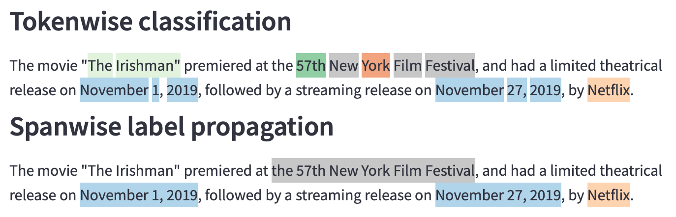
Figure 5: Example NER output of EMBER trained on Ontonotes5 and GPT-2${}_{\text{XL}}$. Colors indicate different predicted entity types. The example illustrates both a failure case due to missed span detection causing correct type predictions to be discarded ("The Irishman", type: "WORK OF ART"), as well as spanwise label propagation applying the correct entity type ("EVENT") to a multi-token span based on the type predicted for the last token ("The 57th New York Film Festival").

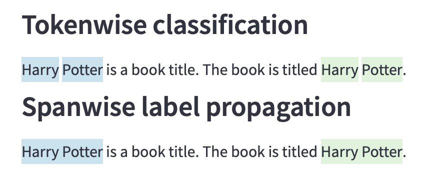
Figure 6: Example NER output of EMBER trained on Ontonotes5 and GPT-2${}_{\text{XL}}$. Colors indicate different predicted entity types (blue: "PERSON", green: "WORK OF ART"). The example illustrates an inherent limitation of our approach due to autoregressivity, where the first mention of "Harry Potter" is misclassified as "PERSON". The second mention is correctly classified as "WORK OF ART" since the required context preceedes the entity mention.

Appendix A Implementation Details

Data and Models. All experiments are performed using the datasets CoNLL2003 Tjong Kim Sang and De Meulder (2003) and Ontonotes5 Hovy et al. (2006) and 7 LMs from the model families GPT-2 Radford et al. (2019), GPT-J Wang and Komatsuzaki (2021), and Pythia Biderman et al. (2023), implemented in Huggingface’s Transformers Wolf et al. (2020) for Python. NER F1 scores are computed using Seqeval Nakayama (2018).

Probing Classifiers. For our probing classifiers, we use a multilayer perceptron (MLP) with a single hidden layer with $n_{\text{neurons}}\in\{32,1024,4096\}$ neurons and ReLU Agarap (2018) as activation function. We find that across all experiments the best results are obtained with $n_{\text{neurons}}=4096$. We use cross-entropy loss and AdamW Loshchilov and Hutter (2019) as optimizer, batch sizes $\in[1024,4096]$ (learning rates $\in[5\mathrm{e}{-4},1\mathrm{e}{-4},5\mathrm{e}{-5}]$) and train using linear warmup (1 epoch) Goyal et al. (2017) followed by a linear learning rate decay. We train tokenwise typing classifiers for $25$ epochs and span detection classifiers for $50$ epochs.

Data formatting. We evaluate results at a tokenized level, meaning that we convert both the texts as well as the labels for CoNLL2003 and Ontonotes5 using the appropriate tokenizers for a given LM. When training probing classifiers, we do not structure our batches according to source data samples, but instead at a "per representation" level: In our implementation we begin by sampling internal LM representations for each token (or attention weight) in the NER dataset and cache the representations. During the training of the probes, we sample from these representations, meaning that for tokenwise classification, a batch size of $n$ corresponds to $n$ hidden states, not $n$ training example texts from CoNLL2003 or Ontonotes5.

Few-Shot Learning. We construct the few-shot task similar to the standard $n$-way $k$-shot setting with $n=4$ dictated by the amount of classes given in the dataset. We evaluate each model for 200 episodes, the support set for each of which is sampled by retrieving $k$ data samples containing at least one mention of each entity type. If a sample contains multiple entity mentions, we also count these towards $k$. In order to use EMBER in this setting, we save the hidden states at a single layer and the attention weights between all tokens in all support data samples. Instead of training probing classifiers, we then perform nearest neighbour classification based on the support representations.

Appendix B Detailed Label Propagation and Span Detection Results for all 7 LMs

Model	P	R	F1
conll2003
Tokenwise typing
GPT-2${}_{\text{small}}$	62.50%	77.90%	69.36%
GPT-2${}_{\text{XL}}$	64.55%	79.10%	71.09%
GPT-J${}_{\text{6B}}$	65.88%	80.24%	72.36%
Pythia${}_{\text{410m}}$	56.90%	74.87%	64.66%
Pythia${}_{\text{1.4b}}$	63.12%	78.04%	69.79%
Pythia${}_{\text{2.8b}}$	63.26%	78.14%	69.91%
Pythia${}_{\text{6.9b}}$	64.46%	79.13%	71.05%
Adj. propagation
GPT-2${}_{\text{small}}$	82.25%	87.68%	84.88%
GPT-2${}_{\text{XL}}$	84.40%	90.47%	87.33%
GPT-J${}_{\text{6B}}$	86.70%	92.02%	89.28%
Pythia${}_{\text{410m}}$	82.86%	88.84%	85.75%
Pythia${}_{\text{1.4b}}$	84.24%	90.39%	87.21%
Pythia${}_{\text{2.8b}}$	86.54%	91.84%	89.11%
Pythia${}_{\text{6.9b}}$	87.50%	92.58%	89.97%
Spanwise typing
GPT-2${}_{\text{small}}$	85.07%	88.34%	86.67%
GPT-2${}_{\text{XL}}$	89.32%	91.75%	90.52%
GPT-J${}_{\text{6B}}$	88.82%	91.60%	90.19%
Pythia${}_{\text{410m}}$	84.44%	87.04%	85.72%
Pythia${}_{\text{1.4b}}$	87.37%	90.22%	88.77%
Pythia${}_{\text{2.8b}}$	88.37%	90.17%	89.26%
Pythia${}_{\text{6.9b}}$	89.13%	91.35%	90.23%
Span propagation
GPT-2${}_{\text{small}}$	92.41%	79.49%	85.46%
GPT-2${}_{\text{XL}}$	94.08%	87.13%	90.47%
GPT-J${}_{\text{6B}}$	94.49%	83.76%	88.80%
Pythia${}_{\text{410m}}$	92.72%	81.61%	86.81%
Pythia${}_{\text{1.4b}}$	93.84%	82.78%	87.96%
Pythia${}_{\text{2.8b}}$	94.30%	85.41%	89.63%
Pythia${}_{\text{6.9b}}$	94.90%	86.05%	90.26%

Table 7: NER scores using hidden states and attention weights in different ways. All scores are micro F1 scores measured on the validation set of CoNLL2003.

Model	P	R	F1
ontonotes5
Tokenwise typing
GPT-2${}_{\text{small}}$	55.69%	69.78%	61.94%
GPT-2${}_{\text{XL}}$	58.56%	71.55%	64.41%
GPT-J${}_{\text{6B}}$	59.52%	72.54%	65.39%
Pythia${}_{\text{410m}}$	54.65%	67.96%	60.58%
Pythia${}_{\text{1.4b}}$	55.98%	69.84%	62.15%
Pythia${}_{\text{2.8b}}$	55.93%	69.92%	62.15%
Pythia${}_{\text{6.9b}}$	57.68%	71.12%	63.70%
Adj. propagation
GPT-2${}_{\text{small}}$	64.39%	72.92%	68.39%
GPT-2${}_{\text{XL}}$	68.25%	76.11%	71.96%
GPT-J${}_{\text{6B}}$	69.64%	77.85%	73.52%
Pythia${}_{\text{410m}}$	68.74%	76.78%	72.54%
Pythia${}_{\text{1.4b}}$	70.21%	77.42%	73.64%
Pythia${}_{\text{2.8b}}$	70.79%	78.10%	74.27%
Pythia${}_{\text{6.9b}}$	70.27%	77.84%	73.86%
Spanwise typing
GPT-2${}_{\text{small}}$	71.57%	76.07%	73.75%
GPT-2${}_{\text{XL}}$	76.79%	76.26%	76.52%
GPT-J${}_{\text{6B}}$	75.22%	75.28%	75.25%
Pythia${}_{\text{410m}}$	73.11%	73.64%	73.37%
Pythia${}_{\text{1.4b}}$	74.00%	73.69%	73.84%
Pythia${}_{\text{2.8b}}$	74.79%	74.54%	74.67%
Pythia${}_{\text{6.9b}}$	75.27%	78.84%	77.01%
Span propagation
GPT-2${}_{\text{small}}$	85.21%	62.31%	71.98%
GPT-2${}_{\text{XL}}$	87.26%	72.77%	79.36%
GPT-J${}_{\text{6B}}$	86.82%	69.88%	77.43%
Pythia${}_{\text{410m}}$	85.29%	68.60%	76.04%
Pythia${}_{\text{1.4b}}$	85.76%	68.46%	76.14%
Pythia${}_{\text{2.8b}}$	86.67%	71.22%	78.19%
Pythia${}_{\text{6.9b}}$	86.81%	72.14%	78.80%

Table 8: NER scores using hidden states and attention weights in different ways. All scores are micro F1 scores measured on the validation set Ontonotes5.

The results of the different label propagation strategies outlined in section 3.3 for all models are given in table 7 for CoNLL2003 and table 8 for Ontonotes5.

	span detection
Model	last	next	adjacency
conll2003
GPT-2${}_{\text{small}}$	85.49%	89.65%	96.62%
GPT-2${}_{\text{XL}}$	91.07%	94.20%	97.64%
GPT-J${}_{\text{6B}}$	90.11%	91.59%	98.00%
Pythia${}_{\text{410m}}$	88.50%	91.04%	97.69%
Pythia${}_{\text{1.4b}}$	88.89%	91.37%	97.84%
Pythia${}_{\text{2.8b}}$	90.83%	93.02%	98.25%
Pythia${}_{\text{6.9b}}$	90.94%	92.99%	98.43%
ontonotes5
GPT-2${}_{\text{small}}$	75.14%	76.56%	89.11%
GPT-2${}_{\text{XL}}$	81.46%	83.92%	91.56%
GPT-J${}_{\text{6B}}$	79.28%	81.27%	91.90%
Pythia${}_{\text{410m}}$	77.07%	80.71%	92.12%
Pythia${}_{\text{1.4b}}$	78.26%	80.73%	92.48%
Pythia${}_{\text{2.8b}}$	79.63%	82.93%	93.21%
Pythia${}_{\text{6.9b}}$	79.99%	83.48%	93.23%

Table 9: Span detection: Micro F1 scores (validation set) for mention detection classifiers trained on attention weights between either last or next token and the first token of a span. Adjacency: Micro F1 scores (validation set) for classifiers using attention weights to classify whether two adjacent tokens belong to the same entity.

The results of the different span detection strategies outlined in section 3.2 are given in table 9. For adjacency classification, we see F1 scores of up to $98.43\%$ on CoNLL2003 and up to $93.23\%$ for Ontonotes5. For the two span classification approaches, we find that predicting $f_{span}(A_{k,i})=\hat{s}_{i,j}$ based on $j=k-1$ ("next") outperforms the alternative, with up to $94.2\%$ for CoNLL2003 and $83.92\%$ for Ontonotes5. Note that these results are obtained on individual data samples (individual representations paired with labels, as used during training) so that the evaluation and metrics calculation is not computed at the sequence level. Therefore these results are not comparable with mention detection scores given in the other experiments, as those are computed using the full EMBER pipelines and at the sequence level.

Appendix C Extended Supervised Learning Benchmark Results

Model	CoNLL2003				Ontonotes5
	$l$	P	R	F1	$l$	P	R	F1
GPT-2${}_{\text{small}}$	8/12	86.66%	72.49%	78.94%	12/12	85.48%	62.02%	71.89%
GPT-2${}_{\text{XL}}$	36/48	89.01%	81.59%	85.14%	30/48	87.80%	72.24%	79.26%
GPT-J${}_{\text{6B}}$	12/28	89.54%	78.54%	83.68%	16/28	87.07%	68.54%	76.70%
Pythia${}_{\text{410m}}$	15/24	87.42%	76.63%	81.67%	14/24	86.08%	68.90%	76.54%
Pythia${}_{\text{1.4b}}$	18/24	88.54%	76.84%	82.27%	16/24	87.13%	68.33%	76.59%
Pythia${}_{\text{2.8b}}$	21/32	89.58%	80.21%	84.63%	17/32	87.66%	72.05%	79.09%
Pythia${}_{\text{6.9b}}$	22/32	89.37%	79.05%	83.90%	19/32	87.44%	71.80%	78.85%

Table 10: Full NER F1 scores for CoNLL2003 and Ontonotes5 using EMBER (spanwise label propagation) in the supervised learning setting. $l$ denotes the layer index at which the hidden states are probed for entity typing (chosen via hyperparameter optimization).

See table 10 for precision, recall, and F1 scores for supervised learning benchmarks across all 7 LMs, as well as the layer index $l$ chosen for entity typing via hyperparameter optimization.

Appendix D Classification Examples

Figures 5 and 6 show examples of prompt annotated with EMBER on GPT-2${}_{\text{XL}}$ and trained on Ontonotes5. The prompt in figure 5 was chosen to show how predicted entity types change as more context information is incorporated into long spans ("The 57th New York Film Festival"), which is previously unavailable to the model due to autoregressivity. The prompt in figure 6 was chosen to highlight an inherent limitation of EMBER due to autoregressivity which can not be fixed using the proposed methods.

Appendix E Model Architecture Details

Model	Hidden dim	# att heads	# layers	$|A|$
GPT-2
GPT-2${}_{\text{small}}$	768	12	12	144
GPT-2${}_{\text{XL}}$	1600	25	48	1200
GPT-J
GPT-J${}_{\text{6B}}$	4096	16	28	448
Pythia
Pythia${}_{\text{410m}}$	1024	16	24	384
Pythia${}_{\text{1.4b}}$	2048	16	24	384
Pythia${}_{\text{2.8b}}$	2560	32	32	1024
Pythia${}_{\text{6.9b}}$	4096	32	32	1024

Table 11: Relevant architecture parameters for models used in experiments.

In table 11, we detail the relevant architecture parameters of the models used in our experiments.

Appendix F Entity Typing based on Last Token

Model	conll2003	ontonotes5
GPT-2${}_{\text{small}}$	93.99%	92.03%
GPT-2${}_{\text{XL}}$	95.46%	92.73%
GPT-J${}_{\text{6B}}$	96.25%	93.45%
Pythia${}_{\text{410m}}$	94.98%	92.75%
Pythia${}_{\text{1.4b}}$	95.59%	93.08%
Pythia${}_{\text{2.8b}}$	95.93%	92.86%
Pythia${}_{\text{6.9b}}$	96.38%	93.02%

Table 12: Entity typing F1 scores (based on last token of a span).

Figure 7: Entity typing F1 scores (validation set) for GPT-2${}_{\text{XL}}$ with respect to the chosen layer.

In table 12 we show results for entity typing where, given the correct spans, we use only the last token of each span to predict its type. We measure F1 scores of up to $96.38\%$ and $93.45\%$, which we argue supports our choice of using a span’s last token for label propagation.

Figure 7 shows a plot of entity typing F1 scores measured using the hidden states at different layers of GPT-2${}_{\text{XL}}$ as feature space. We observe a clear trend showing that representations at earlier layers are less suitable for entity typing, which is in line with the findings of similar previous studies. It is also the basis for choosing layers $2/3$ deep into the LM for the few-shot experiments.

Appendix G Few-Shot NER for GPT-2${}_{\text{small}}$ and Pythia Models

Model	1-shot	5-shot	10-shot	50-shot	100-shot
GPT-2${}_{\text{small}}$	23.67%	34.02%	37.24%	43.81%	48.11%
Pythia${}_{\text{410m}}$	22.52%	34.09%	38.79%	45.07%	46.45%
Pythia${}_{\text{1.4b}}$	23.23%	37.91%	42.44%	50.75%	53.72%
Pythia${}_{\text{2.8b}}$	23.52%	38.29%	41.72%	51.77%	54.66%
Pythia${}_{\text{6.9b}}$	14.11%	25.07%	32.90%	41.83%	47.93%

Table 13: Few-Shot F1 scores for NER on CoNLL2003. All scores are micro F1 scores.

Table 13 shows the few-shot learning results for the remaining models not shown in table 4. We observe that Pythia${}_{\text{6.9b}}$ appears to be an outlier exhibiting particularly low F1 scores. This suggests that there are other factors at play in this particular setting which can not be explained given the variables we measure.

Appendix H Generated NER Datasets

We construct the datasets for section 5 as follows:

Evaluation Dataset. We begin by randomly sampling 50 texts from CoNLL2003. Next we use each text as a prompt for GPT-2${}_{\text{XL}}$ to generate 100 tokens using greedy decoding with a repetition penalty of $1.2$. We manually annotate the generated texts including their prompts (in order to ensure that any potential differences in annotation style do not interfere with the comparison of prompts vs. generated texts) according to the annotation guidelines used for CoNLL2003. The resulting dataset contains 91 entity mentions in the prompts and 297 entity mentions in the generated text.

Synthetic Training Dataset. We generate texts for the training and validation splits of CoNLL2003 in the same way as for the evaluation dataset (excluding the 50 samples used for evaluation from the validation split). Instead of manual annotation, we annotate the texts using the reference model. We train the span detection probe only on the generated portion of each text, amsking out the prompt during feature generation. The remaining training procedure is identical to that used in the supervised learning setting (4.2).

Appendix I Entity Typing and Mention Detection Scores for Generated Text

Data	P	R	F1
entity typing
original	$87.91\%$	$87.91\%$	$87.91\%$
generated	$88.22\%$	$88.22\%$	$88.22\%$
$\Delta$	$+0.30\%$	$+0.30\%$	$+0.30\%$
md - ember
original	$91.95\%$	$87.91\%$	$89.89\%$
generated	$92.86\%$	$70.03\%$	$79.85\%$
$\Delta$	$+0.90\%$	$-17.88\%$	$-10.04\%$
md - ember trained on generated
original	$89.87\%$	$78.02\%$	$83.53\%$
generated	$92.83\%$	$78.45\%$	$85.04\%$
$\Delta$	$+2.96\%$	$+0.43\%$	$+1.51\%$
md - reference
original	$91.40\%$	$93.41\%$	$92.39\%$
generated	$85.43\%$	$86.87\%$	$86.14\%$
$\Delta$	$-5.97\%$	$-6.54\%$	$-6.25\%$

Table 14: Isolated entity typing and mention detection scores measured on generated and non-generated data during experiments outlined in 5.

In table 14 we show entity typing and mention detection scores for generated text in isolation. This data clearly shows that the drop in performance is due to mention detection recall suffering for EMBER trained on non-generated text. Based on these results we retrain only the span detection probe on synthetically annotated generated text.

Appendix J Attention Windowing during Generation

Data	P	R	F1
ember (gpt-2${}_{\text{XL}}$) - windowed
original	$83.72\%$	$79.12\%$	$81.36\%$
generated	$85.04\%$	$67.00\%$	$74.95\%$
$\Delta$	$+1.32\%$	$-12.12\%$	$-6.40\%$
$\Delta$${}_{\text{MD}}$	$-1.57\%$	$-15.86\%$	$-9.79\%$

Table 15: NER scores for windowed attention weights (window size $10$).

During our experiments in simultaneous generation and extraction we hypothesized that another factor, rather than different attention behaviour on generated text, could have caused a model trained on non-generated text to perform poorly on generated text: The generated texts are necessarily longer than the original texts (prompt + generation). Since mention detection is performed based only on the softmax normalized attention weights between two tokens, attention weights may be lower for longer contexts. We, therefore, repeated the measurements obtained with the model trained on non-generated data, this time masking attention weights between tokens at a distance (with the exception of the attention weight directed at token 0 as this is often high regardless of distance) higher than $10$, and find that the drop in recall persists (albeit reduced). The measured results are given in table 15.

References

- Adi et al. (2017) Yossi Adi, Einat Kermany, Yonatan Belinkov, Ofer Lavi, and Yoav Goldberg. 2017. Fine-grained analysis of sentence embeddings using auxiliary prediction tasks.
- Agarap (2018) Abien Fred Agarap. 2018. Deep learning using rectified linear units (relu). CoRR, abs/1803.08375.
- Ashok and Lipton (2023) Dhananjay Ashok and Zachary C. Lipton. 2023. Promptner: Prompting for named entity recognition.
- Belinkov (2022) Yonatan Belinkov. 2022. Probing classifiers: Promises, shortcomings, and advances. Computational Linguistics, 48(1):207–219.
- Belinkov and Glass (2019) Yonatan Belinkov and James Glass. 2019. Analysis methods in neural language processing: A survey. Transactions of the Association for Computational Linguistics, 7:49–72.
- Biderman et al. (2023) Stella Biderman, Hailey Schoelkopf, Quentin Anthony, Herbie Bradley, Kyle O’Brien, Eric Hallahan, Mohammad Aflah Khan, Shivanshu Purohit, USVSN Sai Prashanth, Edward Raff, Aviya Skowron, Lintang Sutawika, and Oskar van der Wal. 2023. Pythia: A suite for analyzing large language models across training and scaling.
- Brown et al. (2020) Tom B Brown, Benjamin Mann, Nick Ryder, Melanie Subbiah, Jared Kaplan, Prafulla Dhariwal, Arvind Neelakantan, Pranav Shyam, Girish Sastry, Amanda Askell, Sandhini Agarwal, Ariel Herbert-Voss, Gretchen Krueger, and Tom Henighan. 2020. Language Models are Few-Shot Learners.
- Cao et al. (2021) Steven Cao, Victor Sanh, and Alexander Rush. 2021. Low-complexity probing via finding subnetworks. In Proceedings of the 2021 Conference of the North American Chapter of the Association for Computational Linguistics: Human Language Technologies, pages 960–966, Online. Association for Computational Linguistics.
- Chen et al. (2023) Jiawei Chen, Yaojie Lu, Hongyu Lin, Jie Lou, Wei Jia, Dai Dai, Hua Wu, Boxi Cao, Xianpei Han, and Le Sun. 2023. Learning in-context learning for named entity recognition. In Proceedings of the 61st Annual Meeting of the Association for Computational Linguistics (Volume 1: Long Papers), pages 13661–13675, Toronto, Canada. Association for Computational Linguistics.
- Chowdhery et al. (2022) Aakanksha Chowdhery, Sharan Narang, Jacob Devlin, Maarten Bosma, Gaurav Mishra, Adam Roberts, Paul Barham, Hyung Won Chung, Charles Sutton, and Sebastian Gehrmann et al. 2022. PaLM: Scaling Language Modeling with Pathways.
- Clark et al. (2019) Kevin Clark, Urvashi Khandelwal, Omer Levy, and Christopher D. Manning. 2019. What does BERT look at? an analysis of BERT’s attention. In Proceedings of the 2019 ACL Workshop BlackboxNLP: Analyzing and Interpreting Neural Networks for NLP, pages 276–286, Florence, Italy. Association for Computational Linguistics.
- Dhuliawala et al. (2023) Shehzaad Dhuliawala, Mojtaba Komeili, Jing Xu, Roberta Raileanu, Xian Li, Asli Celikyilmaz, and Jason Weston. 2023. Chain-of-Verification Reduces Hallucination in Large Language Models.
- Ettinger et al. (2016) Allyson Ettinger, Ahmed Elgohary, and Philip Resnik. 2016. Probing for semantic evidence of composition by means of simple classification tasks. In Proceedings of the 1st Workshop on Evaluating Vector-Space Representations for NLP, pages 134–139, Berlin, Germany. Association for Computational Linguistics.
- Fu et al. (2021) Jinlan Fu, Xuanjing Huang, and Pengfei Liu. 2021. SpanNER: Named entity re-/recognition as span prediction. In Proceedings of the 59th Annual Meeting of the Association for Computational Linguistics and the 11th International Joint Conference on Natural Language Processing (Volume 1: Long Papers), pages 7183–7195, Online. Association for Computational Linguistics.
- Gao et al. (2024) Yunfan Gao, Yun Xiong, Xinyu Gao, Kangxiang Jia, Jinliu Pan, Yuxi Bi, Yi Dai, Jiawei Sun, Qianyu Guo, Meng Wang, and Haofen Wang. 2024. Retrieval-Augmented Generation for Large Language Models: A Survey.
- Geva et al. (2023) Mor Geva, Jasmijn Bastings, Katja Filippova, and Amir Globerson. 2023. Dissecting Recall of Factual Associations in Auto-Regressive Language Models.
- Ghandeharioun et al. (2024) Asma Ghandeharioun, Avi Caciularu, Adam Pearce, Lucas Dixon, and Mor Geva. 2024. Patchscopes: A Unifying Framework for Inspecting Hidden Representations of Language Models.
- Goodfellow et al. (2015) Ian J. Goodfellow, Mehdi Mirza, Da Xiao, Aaron Courville, and Yoshua Bengio. 2015. An Empirical Investigation of Catastrophic Forgetting in Gradient-Based Neural Networks.
- Goyal et al. (2017) Priya Goyal, Piotr Dollár, Ross Girshick, Pieter Noordhuis, Lukasz Wesolowski, Aapo Kyrola, Andrew Tulloch, Yangqing Jia, and Kaiming He. 2017. Accurate, Large Minibatch SGD: Training ImageNet in 1 Hour.
- Guo et al. (2023) Yucan Guo, Zixuan Li, Xiaolong Jin, Yantao Liu, Yutao Zeng, Wenxuan Liu, Xiang Li, Pan Yang, Long Bai, Jiafeng Guo, and Xueqi Cheng. 2023. Retrieval-augmented code generation for universal information extraction.
- Guu et al. (2020) Kelvin Guu, Kenton Lee, Zora Tung, Panupong Pasupat, and Mingwei Chang. 2020. Retrieval augmented language model pre-training. In Proceedings of the 37th International Conference on Machine Learning, volume 119 of Proceedings of Machine Learning Research, pages 3929–3938. PMLR.
- Hernandez et al. (2023) Evan Hernandez, Arnab Sen Sharma, Tal Haklay, Kevin Meng, Martin Wattenberg, Jacob Andreas, Yonatan Belinkov, and David Bau. 2023. Linearity of Relation Decoding in Transformer Language Models.
- Hovy et al. (2006) Eduard Hovy, Mitchell Marcus, Martha Palmer, Lance Ramshaw, and Ralph Weischedel. 2006. OntoNotes: The 90% solution. In Proceedings of the Human Language Technology Conference of the NAACL, Companion Volume: Short Papers, pages 57–60, New York City, USA. Association for Computational Linguistics.
- Htut et al. (2019) Phu Mon Htut, Jason Phang, Shikha Bordia, and Samuel R. Bowman. 2019. Do Attention Heads in BERT Track Syntactic Dependencies?
- Josifoski et al. (2022) Martin Josifoski, Nicola De Cao, Maxime Peyrard, Fabio Petroni, and Robert West. 2022. GenIE: Generative information extraction. In Proceedings of the 2022 Conference of the North American Chapter of the Association for Computational Linguistics: Human Language Technologies, pages 4626–4643, Seattle, United States. Association for Computational Linguistics.
- Keskar et al. (2019) Nitish Shirish Keskar, Bryan McCann, Lav R. Varshney, Caiming Xiong, and Richard Socher. 2019. CTRL: A Conditional Transformer Language Model for Controllable Generation.
- Lewis et al. (2020) Patrick Lewis, Ethan Perez, Aleksandra Piktus, Fabio Petroni, Vladimir Karpukhin, Naman Goyal, Heinrich Küttler, Mike Lewis, Wen-tau Yih, Tim Rocktäschel, Sebastian Riedel, and Douwe Kiela. 2020. Retrieval-augmented generation for knowledge-intensive nlp tasks. In Advances in Neural Information Processing Systems, volume 33, pages 9459–9474. Curran Associates, Inc.
- Li et al. (2022) Jing Li, Aixin Sun, Jianglei Han, and Chenliang Li. 2022. A Survey on Deep Learning for Named Entity Recognition. IEEE Transactions on Knowledge and Data Engineering, 34(1):50–70.
- Li et al. (2023) Peng Li, Tianxiang Sun, Qiong Tang, Hang Yan, Yuanbin Wu, Xuanjing Huang, and Xipeng Qiu. 2023. CodeIE: Large code generation models are better few-shot information extractors. In Proceedings of the 61st Annual Meeting of the Association for Computational Linguistics (Volume 1: Long Papers), pages 15339–15353, Toronto, Canada. Association for Computational Linguistics.
- Loshchilov and Hutter (2019) Ilya Loshchilov and Frank Hutter. 2019. Decoupled Weight Decay Regularization. In Proceedings of the International Conference on Learning Representations 2019, page 18.
- Lu et al. (2022) Yaojie Lu, Qing Liu, Dai Dai, Xinyan Xiao, Hongyu Lin, Xianpei Han, Le Sun, and Hua Wu. 2022. Unified structure generation for universal information extraction. In Proceedings of the 60th Annual Meeting of the Association for Computational Linguistics (Volume 1: Long Papers), pages 5755–5772, Dublin, Ireland. Association for Computational Linguistics.
- Luo et al. (2020) Ying Luo, Fengshun Xiao, and Hai Zhao. 2020. Hierarchical contextualized representation for named entity recognition. Proceedings of the AAAI Conference on Artificial Intelligence, 34(05):8441–8448.
- Mareček and Rosa (2019) David Mareček and Rudolf Rosa. 2019. From balustrades to pierre vinken: Looking for syntax in transformer self-attentions. In Proceedings of the 2019 ACL Workshop BlackboxNLP: Analyzing and Interpreting Neural Networks for NLP, pages 263–275, Florence, Italy. Association for Computational Linguistics.
- Meng et al. (2022) Kevin Meng, David Bau, Alex J. Andonian, and Yonatan Belinkov. 2022. Locating and Editing Factual Associations in GPT. In Advances in Neural Information Processing Systems.
- Nakayama (2018) Hiroki Nakayama. 2018. seqeval: A python framework for sequence labeling evaluation. Software available from https://github.com/chakki-works/seqeval.
- Pimentel et al. (2020) Tiago Pimentel, Josef Valvoda, Rowan Hall Maudslay, Ran Zmigrod, Adina Williams, and Ryan Cotterell. 2020. Information-theoretic probing for linguistic structure. In Proceedings of the 58th Annual Meeting of the Association for Computational Linguistics, pages 4609–4622, Online. Association for Computational Linguistics.
- Radford et al. (2019) Alec Radford, Jeff Wu, Rewon Child, David Luan, Dario Amodei, and Ilya Sutskever. 2019. Language models are unsupervised multitask learners.
- Raganato and Tiedemann (2018) Alessandro Raganato and Jörg Tiedemann. 2018. An analysis of encoder representations in transformer-based machine translation. In Proceedings of the 2018 EMNLP Workshop BlackboxNLP: Analyzing and Interpreting Neural Networks for NLP, pages 287–297, Brussels, Belgium. Association for Computational Linguistics.
- Ram et al. (2023) Ori Ram, Yoav Levine, Itay Dalmedigos, Dor Muhlgay, Amnon Shashua, Kevin Leyton-Brown, and Yoav Shoham. 2023. In-context retrieval-augmented language models. Transactions of the Association for Computational Linguistics, 11:1316–1331.
- Ruder et al. (2019) Sebastian Ruder, Anders Søgaard, and Ivan Vulić. 2019. Unsupervised cross-lingual representation learning. In Proceedings of the 57th Annual Meeting of the Association for Computational Linguistics: Tutorial Abstracts, pages 31–38, Florence, Italy. Association for Computational Linguistics.
- Scao et al. (2022) Teven Le Scao, Angela Fan, Christopher Akiki, Ellie Pavlick, Suzana Ilić, Daniel Hesslow, Roman Castagné, Alexandra Sasha Luccioni, François Yvon, and Matthias Gallé et al. 2022. BLOOM: A 176B-Parameter Open-Access Multilingual Language Model.
- Schick et al. (2023) Timo Schick, Jane Dwivedi-Yu, Roberto Dessì, Roberta Raileanu, Maria Lomeli, Luke Zettlemoyer, Nicola Cancedda, and Thomas Scialom. 2023. Toolformer: Language Models Can Teach Themselves to Use Tools.
- Schouten et al. (2022) Stefan Schouten, Peter Bloem, and Piek Vossen. 2022. Probing the representations of named entities in transformer-based language models. In Proceedings of the Fifth BlackboxNLP Workshop on Analyzing and Interpreting Neural Networks for NLP, pages 384–393, Abu Dhabi, United Arab Emirates (Hybrid). Association for Computational Linguistics.
- Shi et al. (2023) Weijia Shi, Sewon Min, Michihiro Yasunaga, Minjoon Seo, Rich James, Mike Lewis, Luke Zettlemoyer, and Wen-tau Yih. 2023. REPLUG: Retrieval-Augmented Black-Box Language Models.
- Shi et al. (2016) Xing Shi, Inkit Padhi, and Kevin Knight. 2016. Does string-based neural MT learn source syntax? In Proceedings of the 2016 Conference on Empirical Methods in Natural Language Processing, pages 1526–1534, Austin, Texas. Association for Computational Linguistics.
- Tan et al. (2021) Zeqi Tan, Yongliang Shen, Shuai Zhang, Weiming Lu, and Yueting Zhuang. 2021. A sequence-to-set network for nested named entity recognition. In Proceedings of the Thirtieth International Joint Conference on Artificial Intelligence, IJCAI-21, pages 3936–3942. International Joint Conferences on Artificial Intelligence Organization. Main Track.
- Tenney et al. (2019) Ian Tenney, Patrick Xia, Berlin Chen, Alex Wang, Adam Poliak, R Thomas McCoy, Najoung Kim, Benjamin Van Durme, Sam Bowman, Dipanjan Das, and Ellie Pavlick. 2019. What do you learn from context? probing for sentence structure in contextualized word representations. In International Conference on Learning Representations.
- Tjong Kim Sang and De Meulder (2003) Erik F. Tjong Kim Sang and Fien De Meulder. 2003. Introduction to the CoNLL-2003 shared task: Language-independent named entity recognition. In Proceedings of the Seventh Conference on Natural Language Learning at HLT-NAACL 2003, pages 142–147.
- Touvron et al. (2023) Hugo Touvron, Thibaut Lavril, Gautier Izacard, Xavier Martinet, Marie-Anne Lachaux, Timothée Lacroix, Baptiste Rozière, Naman Goyal, Eric Hambro, Faisal Azhar, Aurelien Rodriguez, Armand Joulin, Edouard Grave, and Guillaume Lample. 2023. LLaMA: Open and Efficient Foundation Language Models.
- Wang and Komatsuzaki (2021) Ben Wang and Aran Komatsuzaki. 2021. GPT-J-6B: A 6 Billion Parameter Autoregressive Language Model. https://github.com/kingoflolz/mesh-transformer-jax.
- Wang et al. (2023a) Lean Wang, Lei Li, Damai Dai, Deli Chen, Hao Zhou, Fandong Meng, Jie Zhou, and Xu Sun. 2023a. Label words are anchors: An information flow perspective for understanding in-context learning. In Proceedings of the 2023 Conference on Empirical Methods in Natural Language Processing, pages 9840–9855, Singapore. Association for Computational Linguistics.
- Wang et al. (2023b) Shuhe Wang, Xiaofei Sun, Xiaoya Li, Rongbin Ouyang, Fei Wu, Tianwei Zhang, Jiwei Li, and Guoyin Wang. 2023b. Gpt-ner: Named entity recognition via large language models. arXiv preprint arXiv:2304.10428.
- Wang et al. (2021) Xinyu Wang, Yong Jiang, Nguyen Bach, Tao Wang, Zhongqiang Huang, Fei Huang, and Kewei Tu. 2021. Automated concatenation of embeddings for structured prediction. In Proceedings of the 59th Annual Meeting of the Association for Computational Linguistics and the 11th International Joint Conference on Natural Language Processing (Volume 1: Long Papers), pages 2643–2660, Online. Association for Computational Linguistics.
- Wolf et al. (2020) Thomas Wolf, Lysandre Debut, Victor Sanh, Julien Chaumond, Clement Delangue, Anthony Moi, Pierric Cistac, Tim Rault, Remi Louf, Morgan Funtowicz, Joe Davison, Sam Shleifer, Patrick von Platen, Clara Ma, Yacine Jernite, Julien Plu, Canwen Xu, Teven Le Scao, Sylvain Gugger, Mariama Drame, Quentin Lhoest, and Alexander Rush. 2020. Transformers: State-of-the-art natural language processing. In Proceedings of the 2020 Conference on Empirical Methods in Natural Language Processing: System Demonstrations, pages 38–45, Online. Association for Computational Linguistics.
- Yan et al. (2021) Hang Yan, Tao Gui, Junqi Dai, Qipeng Guo, Zheng Zhang, and Xipeng Qiu. 2021. A unified generative framework for various NER subtasks. In Proceedings of the 59th Annual Meeting of the Association for Computational Linguistics and the 11th International Joint Conference on Natural Language Processing (Volume 1: Long Papers), pages 5808–5822, Online. Association for Computational Linguistics.
- Ye et al. (2022) Deming Ye, Yankai Lin, Peng Li, and Maosong Sun. 2022. Packed levitated marker for entity and relation extraction. In Proceedings of the 60th Annual Meeting of the Association for Computational Linguistics (Volume 1: Long Papers), pages 4904–4917, Dublin, Ireland. Association for Computational Linguistics.
- Zhang (2023) Jiawei Zhang. 2023. Graph-toolformer: To empower llms with graph reasoning ability via prompt augmented by chatgpt. ArXiv, abs/2304.11116.
- Zhang et al. (2022) Susan Zhang, Stephen Roller, Naman Goyal, Mikel Artetxe, Moya Chen, Shuohui Chen, Christopher Dewan, Mona Diab, Xian Li, Xi Victoria Lin, Todor Mihaylov, Myle Ott, Sam Shleifer, Kurt Shuster, Daniel Simig, Punit Singh Koura, Anjali Sridhar, Tianlu Wang, and Luke Zettlemoyer. 2022. OPT: Open Pre-trained Transformer Language Models.