PARMESAN: Parameter-Free Memory Search and Transduction for Dense Prediction Tasks

Abstract

In this work we address flexibility in deep learning by means of transductive reasoning. For adaptation to new tasks or new data, existing methods typically involve tuning of learnable parameters or even complete re-training from scratch, rendering such approaches unflexible in practice. We argue that the notion of separating computation from memory by the means of transduction can act as a stepping stone for solving these issues. We therefore propose PARMESAN (parameter-free memory search and transduction), a scalable transduction method which leverages a memory module for solving dense prediction tasks. At inference, hidden representations in memory are being searched to find corresponding examples. In contrast to other methods, PARMESAN learns without the requirement for any continuous training or fine-tuning of learnable parameters simply by modifying the memory content. Our method is compatible with commonly used neural architectures and canonically transfers to 1D, 2D, and 3D grid-based data. We demonstrate the capabilities of our approach at complex tasks such as continual and few-shot learning. PARMESAN learns up to 370 times faster than common baselines while being on par in terms of predictive performance, knowledge retention, and data-efficiency.

1 Introduction

Figure 1: Overview of our parameter-free transduction method for dense prediction tasks. First, a feature extractor $F$ is applied to a query input $x_{q}$ to obtain hidden representations $(h)_{q}^{l}$ for each level $l$. A memory $M$ stores labeled samples along with their hidden representations $(h)_{j}^{l}$. Our approach then performs a hierarchical search in $M$. The search objective is to find both globally and locally similar nodes compared to the query. In each level $l$, we keep the top-$k$ most similar nodes and retrieve their respective child nodes in level $l-1$. Labels $z_{k}$ from most similar memory nodes are retrieved to obtain an initial, raw prediction. Finally, message passing (MP) is applied to obtain a final prediction $y_{q}$. (Simpson images credit: [107, 90, 91, 108])

For training supervised, task-specific deep learning (DL) models, both data and task are usually well-defined in advance. While this setup holds true for many practical problems, a major issue emerges when already existing models require the ability to adapt to both new data and new tasks. Satisfying such a flexibility requirement is non-trivial in practice, adding yet another level of difficulty to a given problem. Although research in fields like continual learning (CL) and few-shot learning (FSL) resulted in many promising approaches, they still suffer from certain restrictions [8, 102] or focus on a specific problem-niche [66]. Moreover, many proposed solutions are often overly complex and require domain experts for deployment and maintenance.

For example, a well established approach is replay-based training in CL, which uses a memory module for knowledge retention [82, 71, 51, 76]. However, replay training turns out to be quite tricky to do in practice due to several reasons. First, models require a high plasticity in order to learn and unlearn continually, which in turn limits their ability to retain knowledge. Forcing the model to be robust, i.e., retain knowledge via replay training, is thus somewhat contradicting the plasticity requirement to learn new concepts. Second, all relevant knowledge has to be incorporated into the model via training, thereby rendering the available memory capacity irrelevant for inference. Third, the balancing of memory samples and new samples for continual training is non-trivial in practice and often leads to the problem of memory overfitting [51, 6, 99]. Finally, replay does not allow to unlearn specific examples easily, e.g., in case they are not needed anymore. Other CL approaches require repeated training from scratch [66], often rendering them infeasible for practical applications.

We argue that simplicity and flexibility are not necessarily mutually exclusive properties of modern DL approaches. In contrast to common, induction-based approaches, where predictions are inferred from general, learned principles, we embrace transduction [21], which is characterized by reasoning from specific training cases to specific test cases.

Our Work: We propose PARMESAN (parameter-free memory search and transduction), an approach that separates computation from memory and extends transduction to complex, high-dimensional labels for dense prediction tasks while at the same time retaining high flexibility. Our method combines several concepts to perform hierarchical correspondence matching with a memory that contains task-specific, labeled data. Rather than requiring to incorporate all knowledge into learnable parameters, the memory in our method extends the capacity of existing models. We further propose a message passing approach to take advantage of correlations within a query sample.

In general, PARMESAN is parameter-free in the sense that it does not have learnable parameters. Instead, learning can be easily and intuitively performed by non-ML experts via memory consolidation, i.e., adding, removing, or modifying memory samples. Our method allows for fast learning and unlearning of individual examples or parts thereof. Unlike many DL approaches for CL and FSL, our method does not require any continual training or fine-tuning. It therefore neither suffers from parameter-induced forgetting and memory overfitting, nor does it require complicated and energy-hungry training by design.

While we apply our method to 2D images in this work, it canonically transfers to other data dimensionalities such as 3D volumes and 1D sequences, as well as being compatible with spatio-temporal data. We do not impose major restrictions on memory size and allow for flexible memory management. Our method can be applied in combination with common DL architectures and is task-agnostic, i.e., transfers to different dense prediction tasks as well as multi-tasking. Our method can be easily integrated into existing DL architectures, thereby enhancing both flexibility and learning speed.

Our Contributions:

• We propose a flexible, parameter-free transduction method for dense prediction tasks using hierarchical correspondence matching with a memory module.

• We further propose a parameter-free message passing approach to take advantage of intra-query correlations.

• We demonstrate that PARMESAN can be used in combination with common feature extractors.

• We show that our method can be successfully applied to CL and FSL, being on par with commonly used baselines in terms of predictive performance. At the same time, our method learns up to 370 times faster, has stable knowledge retention properties, and is data-efficient. We demonstrate the capabilities of our approach for semantic segmentation and monocular depth estimation on the Cityscapes and JSRT Chest X-ray datasets.

2 Related work

Our method combines concepts from the following fields:

Memory Networks: Recently, the field of memory networks [31, 106, 25, 26, 68] experiences renewed interest. When separating computation and memory [26], some parts of an ML model are responsible for computing, others for storing knowledge. With this notion it is possible to add new information easily, while at the same time being able to treat memory contents as variables. Memory consolidation [23, 3] concerns the strategy for deciding which knowledge to keep in the presence of limited memory resources. Sophisticated memory consolidation methods may include, e.g., novelty search [44], where more informative examples replace less informative examples in memory.

Transduction: Recently, transduction methods experience a revival due to their effectiveness on various classification tasks [2, 37]. One of the most prominent transduction methods is based on k-nearest neighbors (k-NN) [16], which aims to find similar examples w.r.t. common features. Transduction via k-NN was demonstrated to work well for image classification [59], where labeled training samples and their hidden representations are stored in memory. Given a query sample, labels of similar samples are retrieved from memory, followed by a majority voting for prediction. Moreover, k-NN in combination with vision transformers [98, 11] yielded promising results for dense out-of-distribution (OOD) detection [20]. However, making k-NN scalable to dense prediction tasks at high resolutions remains underexplored.

Correspondence Matching: Dense correspondence matching [75, 105, 48] [53, 36, 32, 86, 13] is a fundamental problem in computer vision and often acts as a starting point for various downstream tasks such as optical flow, depth-estimation, etc. In this context, promising methods for improving feature correlation have been proposed [94, 34]. Also, methods for exploiting pyramid features have been introduced for object detection [24, 47] and semantic feature matching [95, 111]. Recently, large-scale foundation models [4] have been applied for one-shot semantic segmentation [49]. Many existing matching approaches use a single reference sample with known correspondences, but typically do not scale well to more than one reference sample. Moreover, most methods rely on specific assumptions commonly found in setups with videos or stereo or multi-view images. In contrast, our proposed method allows matching of arbitrary samples and does not require strong assumptions regarding the presence of correspondences.

Message Passing (MP): Graph neural networks [81, 9, 40] introduced the concept of message passing to DL, where graph nodes are updated depending on received messages from connected nodes. MP was successfully applied, e.g., to various problems in bioinformatics, material science, and chemistry [110, 72].

Continual Learning (CL): The field of CL [93, 73, 92, 61, 8, 102] studies the ability of an ML model to acquire, update, and accumulate knowledge in an incremental manner. This enables models, e.g., to adapt to data-distribution shifts and entirely new tasks. CL is also relevant when frequent re-training is infeasible. Three CL scenarios of increasing difficulty have been proposed [97]: task-incremental (TI), domain-incremental (DI), and class-incremental (CI) CL. The definition of the CI scenario is not limited to classification tasks, but is characterized by the ability of a model to infer which task it is presented with. Prominent approaches for CL include regularization-based methods [41, 46], parameter-isolation methods [54, 80], and replay methods [82, 71, 51, 76]. In contrast to biological neural networks, replay in ML is used for regularizing ML models, where the idea is to learn from new data in tandem with data that is stored in a memory or generated during training. Replay methods can even lead to optimal CL in case of a perfect memory [42].

The notion of knowledge retention and mitigation of forgetting [27] plays a major role in learning. Forgetting is affected by many aspects such as capacity, plasticity, and the quality as well as diversity of training data. The catastrophic forgetting problem in CL [56, 18, 55, 19, 41] refers to learnable parameters adapting to the most recently seen training examples, thereby discarding knowledge from old training examples.

Few-Shot Learning (FSL): Many DL approaches lack the ability to learn efficiently when data is limited. This led to advances in the field of FSL [33], i.e., learning from only a few labeled examples. Available examples are also referred to as support samples. Some methods approach FSL by the means of meta learning [12, 69, 22], where an outer optimization loop learns a strategy for an inner loop, which further adjusts a model to a specific task. The outer loop is performed using large datasets, whereas the inner loop has access to support samples. Another approach to FSL is transfer learning via fine-tuning [15, 60, 100, 1, 45]. Starting from a pre-trained model, learnable parameters or parts thereof are fine-tuned to a specific task using available support samples. Initializing models via pre-training on similar data and tasks typically benefits finding models with high performance after fine-tuning.

Privacy: Common application domains for CL and FSL are autonomous driving and medicine, where data distribution shifts [67] over time are common [87, 64] and data is often scarce. However, storing any kind of personally identifiable data such as patient information in a memory can raise privacy concerns. Even storing hidden representations [29] or detailed, sample-specific labels, raises data-privacy issues due to the possibility of reconstruction attacks [17, 85]. The field of data-free CL [46] has emerged as a viable extension when privacy-preservation is required.

3 Method

We now describe our parameter-free transduction method in more detail (also see Fig. 1). First, we provide an overview of our method and describe the individual components of our model, which consists of a frozen feature extractor, a memory, and a transduction module (Sec. 3.1). Given extracted features of a query input, we perform transductive reasoning by searching for similar features within memory samples and retrieving stored labels (Sec. 3.2). Finally, we take advantage of intra-query correlations via message passing (Sec. 3.3) and further improve predictions by applying test-time augmentation (Sec. 3.4).

3.1 General Setup of PARMESAN

Feature Extraction: Our method requires a pre-trained feature extractor $F$. Let $F$ be a neural network with learnable parameters $\theta$ and consisting of an encoder-like or encoder-decoder-like architecture (e.g., U-Net, ConvNeXt-v2, SwinUNETR, etc.) that delivers a feature pyramid $(h)^{l}$ of hidden representations with levels $l=1,...,n$. We refer to $h^{1}$ as the hidden representation of the first level and $h^{n}$ as the hidden representation of the final level (bottleneck). Individual “pixels” in $(h)^{l}$ with their respective features are referred to as nodes. The total number of nodes for level $l$ is $p^{l}=\prod_{dim}res_{dim}^{l}$, where $dim$ refers to the data dimension and $res^{l}$ to the grid resolutions. Our proposed method is designed with the ability to perform tasks like CL and FSL with frozen parameters $\theta$. One can either pre-train $F$ in a supervised or unsupervised manner, or can use existing pre-trained models. We recommend pre-training $F$ on a dense prediction task in order to enrich features with dense information.

Parameter-free Transduction: Let $X$, $H$, and $Z$ be the input-, latent-, and output spaces, respectively. Densely labeled data is referred to as $(x,z)$ with inputs $x\in X$ and labels $z\in Z$. We define a solver $S:X\rightarrow Z$ as the combination of a feature extractor $F:X\rightarrow H$, a memory $M$, and a parameter-free transduction module $G:H\rightarrow Z$. Given a query input $x_{q}$ and a memory $M$ that stores $m$ labeled samples, $G$ then predicts $y_{q}=G(F(x_{q};\theta),M)$. In essence, $G$ performs hierarchical correspondence matching between a query feature pyramid $(h)_{q}^{l}$ and the memory content, followed by label-retrieval and reduction. We use $M$ for both learning and long-term knowledge retention. Knowledge in $M$ can be modified explicitly, allowing for nuanced and sensible management of what to learn, what to retain, and what to forget. Note that this setup shifts the plasticity-robustness trade-off from learnable parameters $\theta$ with parameter-induced forgetting to $M$ with memory-induced forgetting.

Assumptions: We assume grid-based data structures such as images, volumes, videos, and time series. Although we focus on orthogonal grids in this work, our method can be transferred to irregular, adaptive, and isometric grids. We do not impose any restrictions on label-space growth, such as requiring to pre-define the number of output channels, the number of dimensions, or the numerical data type. When taken to extremes, individual tokens of labels can even represent entire data structures such as sets, series, or graphs.

Privacy Preservation: Our method also extends to privacy-preserving settings, where privacy leaks can be mitigated by storing generated [82] or distilled [103, 28] data in $M$. We do not impose strict requirements for having knowledge about labels, e.g., class segments, and their distribution, e.g., class abundances. This setup even allows for keeping memory labels private if needed.

3.2 Hierarchical Correspondence Matching

We initialize our model by filling $M$ with $m$ labeled samples consisting of $(x,z)_{j}$ as well as their respective feature pyramids $(h)_{j}^{l}$, where $j=1,...,m$ and $l=1,...,n$. Leaf nodes in level $l=0$ refer to memory labels $z_{j}$. Next, we define connectivity kernels which define children-parent relations across different levels. Kernels remain fixed for every sample and for every level. For more details, see Appendix 0.A.

Some neural architectures may not provide desired feature pyramids in the sense that resolutions are halved at every level or that bottlenecks have small resolutions. In these cases, connectivity kernels can either be adjusted accordingly, or missing representations can be inserted by interpolation or extrapolation of neighboring representations.

Algorithm 1 PARMESAN model inference

$dim$, $\phi$ $\triangleright$ hyperparameters

$x_{q},(h)_{j}^{l},z_{j}\ ;j=1,...,m\ ;l=1,...,n$ $\triangleright$ input

$(h)_{q}^{l}\leftarrow F(x_{q};\theta)\ ;l=1,...,n$ $\triangleright$ encode query

init (in parallel for all $p^{n}$ query nodes):

$k\leftarrow m$

$id_{k,par}\leftarrow p^{n}\times[0,1,2,...,k]$ $\triangleright$ parent indices

$s_{k,par}\leftarrow p^{n}\times[1.,1.,1.,...,1.]$ $\triangleright$ parent similarities

memory search (in parallel for all $p^{l}$ query nodes):

for $l=n,1$ do

     $id_{comp}\leftarrow get\_children(l+1,id_{k,par})$ $\triangleright$ [$p^{l}\times k\cdot 2^{dim}$]

     $s^{l}\leftarrow calc\_sim(h_{q}^{l},h_{j}^{l}[id_{comp}])$ $\triangleright$ [$p^{l}\times k\cdot 2^{dim}$]

     $s_{acc}^{l}\leftarrow s^{l}\cdot s_{k,par}$ $\triangleright$ update, [$p^{l}\times k\cdot 2^{dim}$]

     if $l>1$ then

         $k\leftarrow\lfloor\phi\cdot k\rfloor$ $\triangleright$ reduce

     end if

     $id_{keep}\leftarrow get\_topk(s_{acc}^{l},k)$ $\triangleright$ find top-$k$, [$p^{l}\times k$]

     $id_{k,par}\leftarrow id_{comp}[id_{keep}]$ $\triangleright$ update, [$p^{l-1}\times k$]

     $s_{k,par}\leftarrow s_{acc}^{l}[id_{keep}]$ $\triangleright$ update, [$p^{l-1}\times k$]

end for

label-retrieval and reduction:

$id_{z}\leftarrow get\_children(l=1,id_{k,par})$

$y_{q,raw}\leftarrow sum(softmax(s_{k,par})_{k}\cdot z_{j}[id_{z}])_{k}$

return $y_{q,raw}$ $\triangleright$ raw prediction

We formulate the transductive forward pass of our method in Algorithm 1. First, a query $x_{q}$ is encoded via $F$ to obtain $(h)_{q}^{l}$. Then, $G$ takes $(h)_{q}^{l}$ together with memory feature pyramids $(h)_{j}^{l}$ and their respective labels $z_{j}$ as inputs. The overall objective is searching for both globally and locally similar nodes in $M$. Starting from $l=n$, the search objective in each level is first comparing queries $h_{q}^{l}$ with keys $h_{j}^{l}$, followed by retrieving the children of the top-$k$ most similar memory nodes. We use the cosine similarity between nodes’ hidden features as our similarity measure. The accumulated similarity $s_{acc}^{l}$ between two nodes at level $l$ is defined as the product of their similarities $s^{l}$ at level $l$ and the similarities $s_{k,par}$ of their respective parents across all higher levels:

$$s_{acc}^{l}=\prod_{u=l}^{n}sim(h_{q}^{u},h_{j}^{u})=\prod_{u=l}^{n}\frac{h_{q}^{u}\cdot h_{j}^{u}}{\lVert h_{q}^{u}\rVert\ \lVert h_{j}^{u}\rVert}$$ (1)

For each of the $p^{l}$ query nodes, we use $s_{acc}^{l}$ to identify the top-$k$ most similar nodes in level $l$ and retrieve their respective children in level $l-1$. This implies that the top-$k$ most similar nodes in level $l$ become parent nodes for level $l-1$. Children nodes in level $l-1$ are required for processing level $l-1$, thereby forming a hierarchy across levels. The hyperparameter $\phi\in(0.0,1.0]$ controls the number $k$ of top-$k$ nodes to retain for every query node in each level during search. Effectively, $\phi$ is the rate of reduction for $k$ in each level. A variable number of nodes can be retained in different memory samples.

Considering the data dimension $dim$ and the grid resolutions $res^{l}$, exhaustive search would result in a computational complexity of $\mathcal{O}((\prod_{dim}res_{dim}^{l})^{2})$ for level $l$. In contrast, our approach performs search locally and has a computational complexity of only $\mathcal{O}(n_{ch}\cdot(\prod_{dim}res_{dim}^{l}))$ with $n_{ch}$ being the number of child nodes in level $l+1$. Also, since search is performed independently for every query node, our approach can be highly parallelized in practice and is thus scalable to high resolutions and high-dimensional data. Moreover, since $h^{l}$ are strongly correlated across levels, there is a high chance that similarities to query nodes are also strongly correlated across levels. In other words, searching locally pre-filters nodes that are unlikely to be among the top-$k$ most similar nodes as search progresses to the next level.

Memory search results in a dense correspondence map between a query $x_{q}$ and, for every query node, their top-$k$ most similar memory nodes $i_{k,par}$. We use these matches to retrieve task-specific labels $z_{k}$ from $M$. To obtain a raw prediction $y_{q,raw}$, we use the softmax-normalized similarities $s_{k,par}$ of all matches to obtain a weighted average of retrieved labels.

3.3 Intra-Query Transduction via Message Passing

Up until this point we did not exploit any intra-query correlations such as applying geometric priors or enforcing smoothness of predictions. Strong local correlations are common in grid-based data and should be exploited if possible. The simplest variant of intra-query transduction is Gaussian blurring, where local smoothness over neighboring nodes is enforced. However, blurring is not content-aware and can harm performance at certain regions, e.g., at sharp corners or small objects. We therefore propose a content-aware, parameter-free message passing (MP) approach to account for local correlations within the query and achieve pixel-exact predictions. We re-use our hierarchical search without memory content to find the top-$\kappa$ nearest neighbor nodes within the query sample itself. Similarity scores between a query node $i$ and its nearest neighbors $j$ are referred to as edges $e_{ij}$. We then perform MP to refine raw predictions $y_{q,raw}$. Considering a query node state $y_{q,i}$, we define the equations for the edges $e_{ij}$, the aggregated message $\hat{y}_{q,i}$, and the node update from step $t\rightarrow t+1$ as

$$e_{ij}=\frac{exp(s_{acc,j}^{1})}{\sum_{j=1}^{\kappa}exp(s_{acc,j}^{1})}\ ,$$ (2)

$$\hat{y}_{q,i}=\sum_{j=1}^{\kappa}e_{ij}\ y_{q,j}^{t}\ ,$$ (3)

$$y_{q,i}^{t+1}=(1-\lambda)\ y_{q,i}^{t}+\lambda\ \hat{y}_{q,i}\ .$$ (4)

The hyperparameter $\lambda\in(0.0,1.0]$ controls the overall strength of MP per step. We apply Eq. 3 and Eq. 4 repeatedly for all query nodes in level $l=0$ until convergence [113], i.e., when $||y_{q,i}^{t+1}-{y}_{q,i}^{t}||\rightarrow 0$. The resulting prediction $y_{q}$ then contains less artifacts and is spatially more consistent compared to $y_{q,raw}$.

3.4 Test-Time Augmentation

Similar to recent work [36], we perform test-time augmentation (TTA) to resolve small errors. We apply multiple forward passes with down-scaled and reflection-padded variants of $x_{q}$. Registration of down-scaled variants with the original variant is achieved by up-scaling and center-cropping the respective predictions. We obtain a final prediction $y_{q}$ by averaging over all passes.

3.5 Fast Learning

PARMESAN is designed to learn fast in the sense that it does not require training of learnable parameters $\theta$ to perform complex tasks such as CL or FSL. In contrast to other approaches, our method only requires memory consolidation, i.e., saving examples in $M$ and extracting their respective feature pyramids $(h)_{j}^{l}$ in a single forward pass using $F$ with pre-trained, frozen $\theta$. For a given hardware setup, learning speed can be split up into required wall-clock times $\tau_{p}$ and $\tau_{l}$ for pre-training and learning, respectively. We define $\tau_{p}$ on a per-dataset basis and $\tau_{l}$ on a per-sample basis. The total required wall-clock time to learn $n$ training samples is then $T=\tau_{p}+n\cdot\tau_{l}$.

4 Experiments and Results

We demonstrate the capabilities of our method in three groups of experiments:

A0 – A18:

ablation studies for semantic segmentation and monocular depth estimation to demonstrate flexibility (Sec. 4.1, Tab. 1, and Tab. 2),

B0 – B7:

CL experiments for studying knowledge retention properties of our method (Sec. 4.2, Tab. 3, and Tab. 4),

C0 – C7:

FSL experiments to investigate data-efficiency (Sec. 4.3 and Tab. 5).

More details regarding applied models, training and evaluation, as well as qualitative results for all experiments are provided in Sec. 0.B.2.

Our main goal is to improve flexibility and adaptation capabilities of DL models while simplifying and speeding up learning for CL and FSL. Problem-specific methods are expected to outperform more general methods such as ours [57, 104, 101].

Datasets: We use the Cityscapes (CITY) benchmark dataset [7] for semantic segmentation and monocular depth estimation. Semantic segmentation masks comprise fine and coarse labels, whereas disparity maps are provided for depth estimation. We also use the JSRT Chest X-ray dataset [84] for semantic segmentation. We refer to Sec. 0.B.1 for further details.

Method: We employ a U-Net [77] variant as our default DL model and feature extractor. For experiments A11 and A14 we use ConvNeXt Tiny [50] with $\theta$ trained on ADE20K [112]. For all experiments that require $M$, we select memory samples randomly from the training split while keeping the random generation process fixed to ensure comparability. For PARMESAN, we set $m~{}=~{}256$, $\phi=0.5$, apply message passing (MP) and test-time augmentation (TTA), and use both pre-trained U-Net encoder and decoder for feature extraction unless stated otherwise. We use Gaussian blurring with $\sigma=5$ pixels in experiment A2. CL and FSL are performed by memory consolidation of training samples. To obtain memory samples for the privacy-preserving experiment A6, we additionally apply data distillation via linear mixup of two random training samples [109, 43, 83, 70].

Baselines: Joint training (JOINT) refers to training on all available training data, thus representing the default supervised learning setup and the upper bound for CL [97]. Fine-tuning (FT) is a simple, yet strong baseline for FSL [10]. Due to catastrophic forgetting, however, FT is regarded as the lower bound for CL [97]. We further employ memory-based approaches such as classical replay (REPLAY) [82, 71, 51, 76] and greedy-sampling dumb learning (GDUMB) [66] as additional baselines for CL. With GDUMB, training is performed from scratch for each individual CL step, thereby exclusively using memory samples. For consistent and fair comparisons to our method, we implement all baselines and adjust method-specific hyperparameters to our data setup.

Evaluation: We use the mean Intersection over Union of classes ($\text{mIoU}_{\text{cl}}$) and categories ($\text{mIoU}_{\text{cat}}$) as evaluation metrics for semantic segmentation and Root-Mean-Square Error (RMSE) in meters for depth estimation. We report best performances on the CITY validation set and on the JSRT test set, since labels for the CITY test set are not publicly available.

4.1 Ablation Studies

We perform ablation studies of various components to analyze the impact on learning speed and predictive performance, as well as demonstrating the flexibility of our method with different architectures of $F$. We summarize our results in Tab. 1 (segmentation) and Tab. 2 (depth) and visualize predictions in Fig. 2 (CITY, segmentation), Fig. 3 (CITY, depth), and Fig. 4 (JSRT, segmentation).

Learning with our method can be done in less than 0.1 seconds per sample (see column $\tau_{l}$ in Tab. 1 and Tab. 2), thereby mitigating the demand for additional computational costs when attaching PARMESAN to existing models. Our method outperforms JOINT on CITY when trained on coarse labels (A9, A10) and evaluated on fine labels. As expected, our method under-performs JOINT when using fine labels (A0, A1), on JSRT (A12, A13, A14), and for depth estimation (A15, A16). Using only the encoder (A7) or using an entirely untrained, randomly initialized model (A8) yields promising results already, indicating that our transduction module $G$ imposes useful inductive biases. PARMESAN can be successfully used in combination with a ConvNeXt feature extractor on both CITY and JSRT when trained on ADE20K [50] (A11, A14). MP and TTA (A1, A3, A4, A16, A17) considerably improve performance over raw predictions (A5, A18). As expected, content-aware MP (A1) also outperforms non-content-aware Gaussian blurring (A2). Comparing panels A1 and A5 in Fig. 2, MP and TTA succeed in reducing small artifacts while retaining sharp corners of predicted segments. In contrast, blurring typically comes at the cost of missing small segments and sharp corners. Privacy-preservation by data distillation (A6) slightly decreases performance compared to the non-private setup (A1).

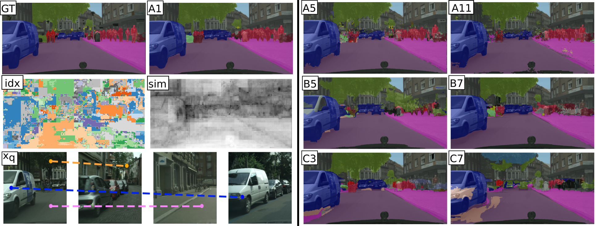
Figure 2: Model predictions and analysis of PARMESAN. Left: We study top-$1$ nearest neighbors from experiment A1. The idx panel visualizes indices of retrieved nearest neighbor nodes from $M$. Similar colors indicate that nodes are retrieved from close-by memory locations, most likely from within the same samples. The sim panel visualizes the respective similarity scores, where bright regions refer to high similarities. We also show 3 query pixels and their matches in $M$, indicating both global and local semantic correspondence. Right: PARMESAN can be applied flexibly (A5, A11) and perform complex tasks like CL (B5, B7) and FSL (C3, C7) via memory consolidation.

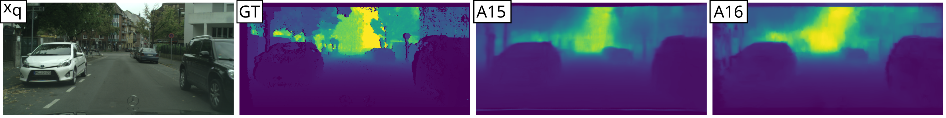
Figure 3: Model predictions for monocular depth estimation experiments.

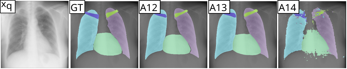
Figure 4: Model predictions for semantic segmentation experiments using JSRT data.

In general, we observe global and local semantic correspondence of retrieved nearest neighbors from $M$, allowing for future work on various topics related to interpretability and explainability of predictions. Moreover, since every retrieved node comes with its similarity score w.r.t. the query, our method provides pixel-exact indications for uncertainty. As visible in the sim panel in Fig. 2, similarity scores seem to be correlated with the heterogeneity of regions in the image.

Table 1: Results for ablation studies showing semantic segmentation performance for classes ($\text{mIoU}_{\text{cl}}$) and categories ($\text{mIoU}_{\text{cat}}$). Column “$F$ pre-train/train“ indicates if the method uses a pre-trained feature extractor $F$ and if any additional training of learnable parameters $\theta$ is required. $\tau_{p}$ and $\tau_{l}$ are wall-clock times for pre-training and learning, respectively. Experiment IDs marked with * use ConvNeXt pre-trained on ADE20K [50] for feature extraction.

ID	Train data (#samples)	Method & Setup	$F$ pre-train/train	$\tau_{p}$ [h]	$\tau_{l}$ [s]	$\text{mIoU}_{\text{cl}}$	$\text{mIoU}_{\text{cat}}$
A0	CITY, fine (2975)	JOINT	no / yes	0	3.72	82.5	87.4
A1	CITY, fine (256)	ours	A0 / no	3.08	0.09	80.0	85.5
A2	CITY, fine (256)	ours, no MP, blur	A0 / no	3.08	0.09	79.3	84.8
A3	CITY, fine (256)	ours, no TTA	A0 / no	3.08	0.09	77.7	83.5
A4	CITY, fine (256)	ours, no MP	A0 / no	3.08	0.09	77.9	83.2
A5	CITY, fine (256)	ours, no MP, no TTA	A0 / no	3.08	0.09	75.7	81.6
A6	CITY, fine (256)	ours, private	A0 / no	3.08	0.10	77.6	83.2
A7	CITY, fine (256)	ours	A0 (E only) / no	3.08	0.08	72.8	79.1
A8	CITY, fine (256)	ours	no / no	0	0.09	56.1	63.5
A9	CITY, coarse (19998)	JOINT	no / yes	0	0.43	49.6	50.6
A10	CITY, coarse (256)	ours	A9 / no	2.41	0.09	50.7	52.5
A11*	CITY, fine (256)	ours	E only / no	-	0.09	74.5	81.4
A12	JSRT (199)	JOINT	no / yes	0	23.39	93.3	-
A13	JSRT (199)	ours, $m\!=\!199$, $\phi\!=\!0.8$	A12 / no	1.29	0.02	91.9	-
A14*	JSRT (199)	ours, $m\!=\!199$, $\phi\!=\!0.8$	E only / no	-	0.02	87.2	-

Table 2: Results for ablation studies showing depth estimation performance.

ID	Train data (#samples)	Method & Setup	$F$ pre-train/train	$\tau_{p}$ [h]	$\tau_{l}$ [s]	RMSE [m]
A15	CITY, disparity (2975)	JOINT	no / yes	0	6.71	10.5
A16	CITY, disparity (256)	ours	A15 / no	5.55	0.03	11.9
A17	CITY, disparity (256)	ours, no MP	A15 / no	5.55	0.03	12.5
A18	CITY, disparity (256)	ours, no MP, no TTA	A15 / no	5.55	0.03	13.5

4.2 Continual Learning

We perform CI-CL experiments, where the goal is to incrementally learn new semantic classes while at the same time automatically inferring the given task. We split the dataset into a total of 4 CL steps where data at every CL step comprises labels for all classes of different categories: $\textit{D}_{1}$: void & flat, $\textit{D}_{2}$: construction & object, $\textit{D}_{3}$: nature & sky, and $\textit{D}_{4}$: human & vehicle. For memory-based methods GDUMB, REPLAY, and PARMESAN, we update samples in $M$ with labels from the current CL step while keeping the stored inputs. GDUMB and REPLAY utilize $M$ for training $\theta$, whereas PARMESAN uses $M$ for transduction. More information about our CL setup is provided in Sec. 0.B.3. We summarize our CL results in Tab. 3 and Tab. 4.

Table 3: Results for CL experiments. Performance is measured on all classes after the final CL step (i.e., after 4 steps). Our method is on-par with CL baselines while learning substantially faster.

ID	Train data (#samples)	Method & Setup	$F$ pre-train/train	$\tau_{p}$ [h]	$\tau_{l}$ [s]	$\text{mIoU}_{\text{cl}}$	$\text{mIoU}_{\text{cat}}$
B0	CITY, fine (2975)	JOINT (upper bound)	no / yes	0	20.62	81.7	86.6
B1	CITY, fine (2975)	FT (lower bound)	no / yes	0	12.76	4.0	4.3
B2	CITY, fine (2975)	REPLAY, $m\!=\!256$	no / yes	0	5.11	56.2	64.2
B3	CITY, fine (256)	GDUMB, $m\!=\!256$	no / yes	0	110.9	74.4	80.3
B4	CITY, fine (256)	ours	B0 ($1^{\text{st}}$ step) / no	3.07	0.32	66.0	70.7
B5	CITY, fine (256)	ours	B3 ($1^{\text{st}}$ step) / no	1.42	0.32	65.4	71.0
B6	CITY, fine (256)	GDUMB, $m\!=\!256$	A9 / yes	2.41	63.13	76.9	82.1
B7	CITY, fine (256)	ours	A9 / no	2.41	0.32	75.4	81.3

Table 4: Forgetting behavior of CL methods after 4 CL steps, showing absolute changes $\delta$ between initial and final $\text{mIoU}_{\text{cl}}$. Each dataset $\textit{D}_{i}$ comprises semantic classes of different categories according to the respective CL step. Our method has stable knowledge retention and can not suffer from parameter-induced forgetting by design.

	REPLAY (B2)		GDUMB (B3)		ours (B4)		ours (B5)		GDUMB (B6)		ours (B7)
$\textit{D}_{i}$	initial	$\delta$	initial	$\delta$	initial	$\delta$	initial	$\delta$	initial	$\delta$	initial	$\delta$
$\textit{D}_{1}$	73.97	-11.23	75.18	-1.52	68.15	-0.58	65.81	-0.56	77.59	-1.26	70.95	-0.51
$\textit{D}_{2}$	39.97	-9.11	49.67	-0.06	31.57	+0.60	33.26	+0.42	54.11	-1.85	49.41	-0.43
$\textit{D}_{3}$	47.55	+3.65	63.72	-0.71	40.65	-0.21	42.06	-0.20	67.59	-0.15	62.05	-0.18
$\textit{D}_{4}$	26.86	-	40.06	-	32.34	-	29.71	-	44.16	-	39.58	-

As expected, FT experiences strong parameter-induced forgetting resulting in $\text{mIoU}_{\text{cl}}=0.0$ on old data (B1). In contrast, JOINT has access to both old and current data, thus outperforming all other methods (B0). Our method outperforms REPLAY (B2) when pre-training $\theta$ solely on $\textit{D}_{1}$ (B4), and even when pre-training on only $m=256$ samples (B5). Similar performances of B4 and B5 indicate that pre-training with a small amount of data suffices in order to apply PARMESAN successfully. Although GDUMB (B3) outperforms our method in terms of overall performance, we demonstrate that PARMESAN has stable knowledge retention properties over all CL steps (see Tab. 4) while at the same time learning 346 times faster. Initializing $\theta$ via pre-training on coarse labels (B6, B7) reduces the performance gap to GDUMB while keeping knowledge retention and fast learning properties. Stable knowledge retention for PARMESAN can be attributed to our shift towards memory-induced forgetting, where we explicitly state what to learn (new classes), what to retain (old classes), and what to forget (background class).

4.3 Few-Shot Learning

For FSL, we pre-train $F$ on coarse labels (A9). We then perform experiments with 10, 8, 6, 4, and 2 fine-labeled support samples. FSL via FT is performed by fine-tuning $\theta$ on support samples. To study FT under realistic conditions, we divide the support sets into 2 splits with the latter containing 4 samples used for early stopping. For FSL with PARMESAN, we fill $M$ with all support samples. A low number of support samples can lead to a high variance in performance. We thus repeat each experiment 5 times with randomly drawn support samples, where we fix the random generation process across experiments to ensure comparability. We report average performances on the full validation set in Tab. 5.

Table 5: Results for FSL experiments, averaged over 5 repetitions. We use a feature extractor pre-trained on coarse labels and a support set containing fine labels. Our method learns fast and is data-efficient especially for small support sets.

ID	Train data (#samples)	Method & Setup	$F$ pre-train/train	$\tau_{p}$ [h]	$\tau_{l}$ [s]	$\text{mIoU}_{\text{cl}}$	$\text{mIoU}_{\text{cat}}$
C0	CITY, fine (10, train on 6)	FT	A9 / yes	2.41	32.29	71.7	76.4
C1	CITY, fine (8, train on 4)	FT	A9 / yes	2.41	69.53	71.1	75.9
C2	CITY, fine (6, train on 2)	FT	A9 / yes	2.41	225.6	69.5	74.7
C3	CITY, fine (10)	ours, $m\!=\!10$, $\phi\!=\!1$	A9 / no	2.41	0.17	72.2	78.2
C4	CITY, fine (8)	ours, $m\!=\!8$, $\phi\!=\!1$	A9 / no	2.41	0.21	71.1	77.5
C5	CITY, fine (6)	ours, $m\!=\!6$, $\phi\!=\!1$	A9 / no	2.41	0.26	69.9	76.2
C6	CITY, fine (4)	ours, $m\!=\!4$, $\phi\!=\!1$	A9 / no	2.41	0.34	66.9	73.3
C7	CITY, fine (2)	ours, $m\!=\!2$, $\phi\!=\!1$	A9 / no	2.41	0.61	58.3	65.6

FSL with PARMESAN can be done up to 370 times faster w.r.t. FT (C2, C7) and remains on par in terms of predictive performance for equal support set sizes (C0-C5). Our method is data-efficient in the sense that is able to utilize the entire support set at inference and that it can be applied in combination with a small support set (C6, C7).

4.4 Limitations

Depending on the choice of hyperparameters such as $m$ and $\phi$, PARMESAN might require more computational resources and longer inference times compared to learned task-heads. Memory consumption and inference speed can potentially be further improved by introducing sparsity to stored feature pyramids, i.e., reducing the number of unique patterns per memory sample. Moreover, choosing a suitable feature extractor might require taking a trade-off between a general-purpose model versus a data- and task-specific model.

5 Conclusion

In this work we proposed PARMESAN, a flexible, parameter-free approach that separates computation from memory and leverages transduction for solving dense prediction tasks. We also proposed a message passing approach to take advantage of intra-query correlations. Our method can perform complex tasks such as CL and FSL in an easy, intuitive, and optionally private manner without any continuous training of learnable parameters.

We demonstrated that our approach learns substantially faster than common baselines while achieving competitive predictive performance, showing stable knowledge retention, and being data-efficient.

Future Work: Possible future work includes leveraging self-supervised feature extractors, studying OOD detection capabilities, as well as investigating memory-related topics such as dataset distillation. Performance might be further increased by implementing algorithmic or methodical improvements. This includes, e.g., using explorative memory search instead of our current greedy approach, as well as applying novelty search instead of random sampling for memory consolidation. Finally, PARMESAN might be beneficial to other fields such as reinforcement learning, where fast adaptation can be important.

Supplementary Material

Philip Matthias Winter, Maria Wimmer, David Major, Dimitrios Lenis, Astrid Berg, Theresa Neubauer, Gaia Romana De Paolis, Johannes Novotny, Sophia Ulonska, Katja Bühler

Appendix 0.A Method

Initialization: We now describe the initialization of $G$ in more detail. First, we need to initialize hyperparameters such as the number of data dimensions $dim$, the number of memory samples $m$ and the resolutions $(res)^{l}$ for all levels. We then define connectivity kernels between nodes of different levels, which remain fixed for all samples. Each node in level $l$ has a parent node in level $l+1$. For the highest level $l=n$, all nodes have a single root node as their parent. Each node in level $l$ typically has several child nodes in level $l-1$, e.g., $n_{ch}=2^{dim}$. Leaf nodes in level $l=0$ refer to memory labels. We assume that resolutions of $h^{1}$, $x$, and $z$ match, implying that each node in level $l=1$ has exactly one child node in $l=0$. We initialize parent indices $i_{k,par}$ such that hierarchical search has access to the full memory content. We initialize parent similarity scores $s_{k,par}$ with a value of 1.0 for all nodes.

Technical Aspects: In order to avoid increasingly exhaustive search due to a rapidly growing number of nodes, we set $\phi$ such that hardware memory requirements remain quasi-constant across levels. For example, $\phi=0.5$ for 2D data in combination with doubling the channel dimension in each level yields quasi-constant hardware memory usage. The same is true for 3D data and $\phi=0.25$. This is especially relevant in case of high-dimensional data and high resolutions, where available hardware often imposes hard limits on the choice of hyperparameters. Naturally, smaller $m$ allow for larger $\phi$. For depth estimation with PARMESAN, we ignore invalid labels in $M$ by manually setting their respective similarity scores $s_{k,par}=-100.0$ before applying the softmax operation.

We implemented all methods and experiments using the PyTorch framework [63]. We apply the exact same pre- and postprocessing to retain comparability. We conduct all experiments on a single NVIDIA GeForce RTX 3090 (24 GB) graphics card. PARMESAN has inference times in the order of 1 second per image for $m=256$, $\phi=0.5$, and an input resolution of 512$\times$1024 pixels. By default, we store memory content on RAM and transfer representations to GPU when needed for hierarchical search. In case of small GPU RAM, the hierarchical search can be chunked into smaller pieces via windowing and performed sequentially without compromising performance. For MP, all operations can be done on GPU.

Appendix 0.B Experiments

0.B.1 Datasets

From the Cityscapes semantic segmentation benchmark dataset (CITY) [7], we use the 5000 images with fine semantic and disparity annotations, and the 19998 images with coarse semantic annotations (see Fig. 5). We use the official splits for training and validation with 2975 and 500 samples, respectively. Since labels for the 1525 test samples are not publicly available, we report best performances achieved on the validation split. For JSRT [84], a 80:10:10 split is applied, resulting in 199, 24, and 24 samples for training, validation, and testing, respectively. For CITY, we use 34 semantic classes with 8 categories for training and the official 19 classes for evaluation. For JSRT, we use 6 classes for training and evaluation: background, left lung, right lung, heart, left clavicle, and right clavicle. We rescale all samples to a resolution of 512$\times$1024 pixels for CITY and 512$\times$512 pixels for JSRT.

For CITY disparity maps, we observe that some pixels near image borders are labeled incorrectly. We manually mask out these erroneous labels and treat them as invalid measurements.

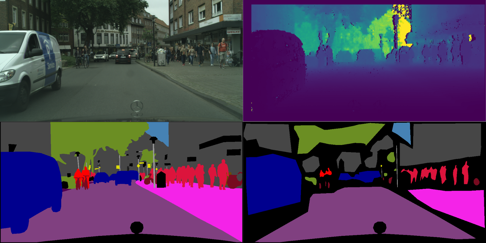
Figure 5: Annotations of Cityscapes dataset (original image, depth map, fine semantic map, coarse semantic map). While coarse annotations only outline the most prominent objects via polygons, pixel-exact fine annotations are regarded as the ground truth.

0.B.2 Models, Methods, Training and Evaluation

Models: We use a U-Net [77] variant with residual blocks [30] and instance normalization [96] as our default architecture, resulting in 9 levels (excluding the label-level $l=0$) with respective feature map resolutions of $[512$, $256$, $128$, $64$, $32$, $16$, $8$, $4$, $2]$ pixels per dimension. The respective number of feature maps are $[6$, $12$, $24$, $48$, $96$, $192$, $384$, $768$, $1536]$, resulting in a total of 73.15m learnable parameters.

For ablations studies, we additionally use a ConvNeXt Tiny with pre-trained weights for feature extraction [50]. Pre-trained weights were obtained by training ADE20K [112] for semantic segmentation. The model comprises 4 levels with feature map resolutions of $[128,64,32,16]$ and corresponding number of feature maps $[96,192,384,786]$. To be able to use it with our transduction module, we complete the feature pyramid, i.e., add missing resolutions, via interpolation and extrapolation of neighboring representations. We reduce the number of feature maps in high resolutions by a factor of 4 to meet our hardware limitations (see paragraph “Training“ below) and keep the number of feature maps constant for missing lower resolutions. This results in $[6,24,96,192,384,768,768,768,768]$ feature maps at the respective resolutions of $[512,256,128,64,32,16,8,4,2]$.

Method: For memory search, we set $n_{ch}=2^{dim}$ for all levels. For MP, we set $\lambda=1$, $k=16$. Convergence is typically achieved within 16 MP steps. For TTA, we apply three separate forward passes and down-scale inputs by factors $s=\{0.8,0.9,1\}$, where $s=1$ implies no transformation.

Training: Some of our experiments (baseline methods and pre-training for PARMESAN) require training of learnable parameters $\theta$. We use the cross-entropy loss as the default loss function for semantic segmentation. For monocular depth estimation, we regress $d:=\textit{log}\textit{(depth)}$ and use the scale-invariant loss [14] with $\lambda=0.5$. We mask out invalid labels both during training and evaluation. Training is performed via stochastic gradient descent [74], utilizing the backpropagation algorithm [38, 78] and the AdamW optimizer [39, 52] with default hyperparameters, a minibatch size of 8, a constant learning rate of 0.0001, and a weight decay of 0.00001. We apply gradient-norm clipping [62], allowing maximum gradient norms of 50. We train our models on randomly cropped patches of 512$\times$512 pixels for CITY and on full images of 512$\times$512 pixels for JSRT. For data augmentation during training, we use horizontal flips ($p=0.5$, not for JSRT), vertical flips ($p=0.5$, not for JSRT), rotations ($p=0.5$, $\pm 25^{\circ}$), Gaussian noise ($p=0.5$, $\sigma=0.05$), as well as changes in brightness, saturation, and contrast.

Evaluation: We use exponential moving average models [65, 79, 89] with a rate of 0.99 for evaluation. Early stopping [58] with a patience of 3 and a validation verbosity of 3000 update steps is used (400 for JSRT). Early stopping in CL experiments only depends on the performance on available classes at the respective CL step. We use a validation verbosity of 30 update steps for FSL FT experiments due to small support sets.

We use the Intersection over Union (IoU) [35, 88] as evaluation metric for semantic segmentation, which is defined as the ratio between the size of the intersection and the size of the union of two finite sample sets, measuring their similarity. In this work, we use IoU to measure predictive performance of a model for the task of pixel-wise, multi-class classification, i.e., semantic segmentation. We employ the standard evaluation procedure as defined in [7]. Specifically, we apply the mean IoU ($\text{mIoU}_{\text{}}$), where scores are calculated globally without favoring any class in particular. This variant is also referred to as “micro”-averaging.

Results: We show qualitative prediction results for all ablation studies, CL experiments, and FSL experiments in Fig. 6, Fig. 7, and Fig. 8, respectively.

0.B.3 Continual Learning Setup

The goal in CL is learning a sequence of $N$ tasks $\mathcal{T}=((T_{1},\textit{D}_{1}),...,(T_{N},\textit{D}_{N}))$ on respective datasets $\mathcal{D}=(\textit{D}_{1},...,\textit{D}_{N})$. Old data $\textit{D}_{j}$ is inaccessible for CL step $i$ for $j<i$. For memory-based CL methods, data from $\textit{D}_{j}$ can still be retained if it is stored in $M$. Given a task-solving model (”solver”) $S:X\rightarrow Z$ with inputs $x\in X$, predictions $y\in Z$, and labels $z\in Z$, the objective is minimizing the unbiased sum of losses $\mathbb{E}_{x,z}[L(y,z)]_{\mathcal{T}}$ over all tasks on the entire data distribution.

In contrast to image classification, samples can contain classes that belong to different CL steps, which is referred to as overlapping labels. For the CI-CL scenario, this requires introducing a dedicated background class to avoid data-leakage between different CL steps. Therefore, non-available classes are re-labeled as background in each CL step. This implies that the background class is different for different CL steps. As proposed in recent work [5], we ignore background pixels for validation.

Our method supports any combination of the three CL scenarios TI, DI, and CI. Although we focus on studying the offline CL scenario in this paper, our method can also be used for online CL, where one does not have access to the entire dataset of a specific task in order to learn continually.

In our experiments, we apply classical replay (REPLAY) as a baseline method. In order to keep labels consistent for replay training, we employ an adaptive masking approach. For samples of the current CL step $i$, we mask out all background pixels, i.e., pixels which do not belong to currently active classes. In contrast, for memory samples we mask out all pixels which belong to currently active classes, i.e., keeping pixels of old classes and the background. Training minibatches for REPLAY consist of standard samples in addition to replay samples, which we select randomly from $M$. For REPLAY, we observe that using one or more replay samples from $M$ per update step leads to strong memory overfitting, which in turn leads to reduced validation performance. We achieve best results with one replay sample every other minibatch.

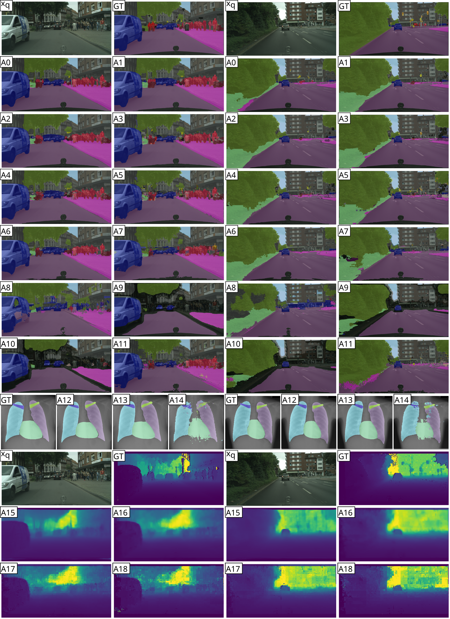
Figure 6: Model predictions for all ablation studies with two different query inputs.

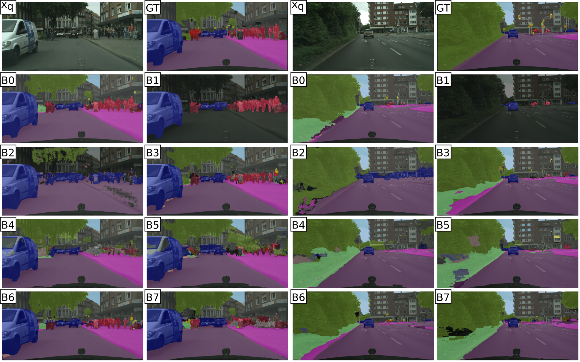
Figure 7: Model predictions for all CL experiments with two different query inputs.

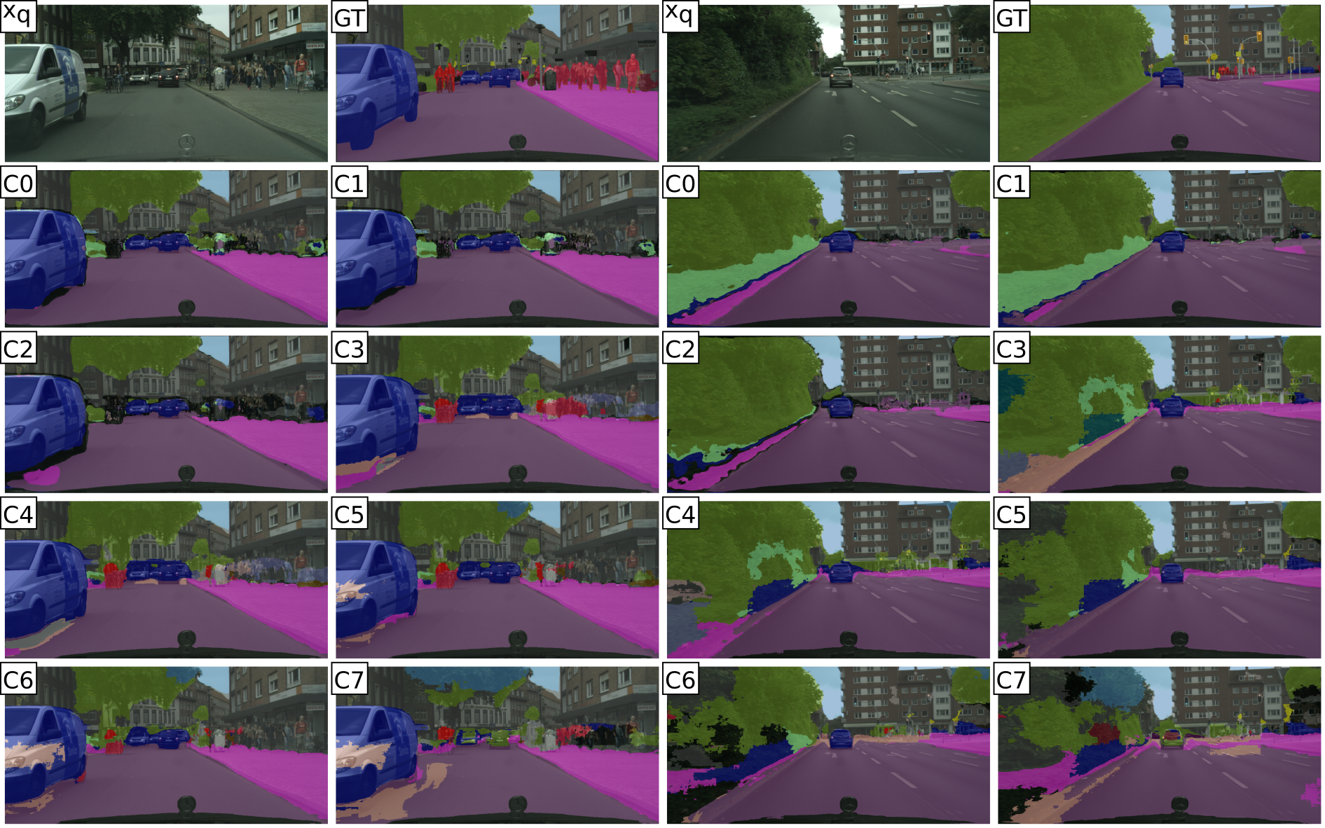
Figure 8: Model predictions for all FSL experiments with two different query inputs.

References

- [1] T. Adler, J. Brandstetter, M. Widrich, A. Mayr, D. P. Kreil, M. Kopp, G. Klambauer, and S. Hochreiter. Cross-domain few-shot learning by representation fusion. CoRR, abs/2010.06498, 2020.
- [2] O. Belhasin, G. Bar-Shalom, and R. El-Yaniv. TransBoost: Improving the best ImageNet performance using deep transduction. In A. H. Oh, A. Agarwal, D. Belgrave, and K. Cho, editors, NeurIPS, volume 35, pages 28363–28373, 2022.
- [3] M. K. Benna and S. Fusi. Computational principles of synaptic memory consolidation. Nature Neuroscience, 19(12):1697—1706, 2016.
- [4] R. Bommasani, D. A. Hudson, E. Adeli, R. Altman, S. Arora, S. von Arx, M. S. Bernstein, J. Bohg, A. Bosselut, E. Brunskill, et al. On the opportunities and risks of foundation models. arXiv preprint, arXiv:2108.07258, 2021.
- [5] F. Cermelli, M. Mancini, S. R. Bulò, E. Ricci, and B. Caputo. Modeling the background for incremental learning in semantic segmentation. In CVPR, pages 9230–9239, 2020.
- [6] A. Chaudhry, M. Rohrbach, M. Elhoseiny, T. Ajanthan, P. K. Dokania, P. H. S. Torr, and M. Ranzato. Continual learning with tiny episodic memories. In Workshop on Multi-Task and Lifelong Reinforcement Learning, 2019.
- [7] M. Cordts, M. Omran, S. Ramos, T. Rehfeld, M. Enzweiler, R. Benenson, U. Franke, S. Roth, and B. Schiele. The cityscapes dataset for semantic urban scene understanding. In CVPR, pages 3213–3223, 2016.
- [8] M. De Lange, R. Aljundi, M. Masana, S. Parisot, X. Jia, A. Leonardis, G. Slabaugh, and T. Tuytelaars. A continual learning survey: Defying forgetting in classification tasks. IEEE TPAMI, 44(07):3366–3385, 2022.
- [9] M. Defferrard, X. Bresson, and P. Vandergheynst. Convolutional neural networks on graphs with fast localized spectral filtering. In D. Lee, M. Sugiyama, U. Luxburg, I. Guyon, and R. Garnett, editors, NeurIPS, volume 29, pages 3837–3845, 2016.
- [10] G. S. Dhillon, P. Chaudhari, A. Ravichandran, and S. Soatto. A baseline for few-shot image classification. In ICLR, 2020.
- [11] A. Dosovitskiy, L. Beyer, A. Kolesnikov, D. Weissenborn, X. Zhai, T. Unterthiner, M. Dehghani, M. Minderer, G. Heigold, S. Gelly, J. Uszkoreit, and N. Houlsby. An image is worth 16x16 words: Transformers for image recognition at scale. In ICLR, 2021.
- [12] V. Dumoulin, N. Houlsby, U. Evci, X. Zhai, R. Goroshin, S. Gelly, and H. Larochelle. A unified few-shot classification benchmark to compare transfer and meta learning approaches. In Proceedings of the Neural Information Processing Systems Track on Datasets and Benchmarks 1, 2021.
- [13] J. Edstedt, Q. Sun, G. Bökman, M. Wadenbäck, and M. Felsberg. RoMa: Revisiting robust losses for dense feature matching. arXiv preprint, arXiv:2305.15404, 2023.
- [14] D. Eigen, C. Puhrsch, and R. Fergus. Depth map prediction from a single image using a multi-scale deep network. In NeurIPS, volume 27, pages 2366–2374, 2014.
- [15] C. Finn, P. Abbeel, and S. Levine. Model-agnostic meta-learning for fast adaptation of deep networks. In ICML, ICML’17, pages 1126–1135, 2017.
- [16] E. Fix and J. L. Hodges. Discriminatory analysis. nonparametric discrimination: Consistency properties. Technical Report Number 4, USAF School of Aviation Medicine, Randolph Field, 1951.
- [17] M. Fredrikson, S. Jha, and T. Ristenpart. Model inversion attacks that exploit confidence information and basic countermeasures. In 22nd ACM SIGSAC Conference on Computer and Communications Security, CCS ’15, pages 1322–1333, 2015.
- [18] R. M. French. Catastrophic interference in connectionist networks: Can it be predicted, can it be prevented? In NeurIPS, pages 1176–1177, 1993.
- [19] R. M. French. Catastrophic forgetting in connectionist networks. Trends in Cognitive Sciences, 3(4):128–135, 1999.
- [20] S. Galesso, M. Argus, and T. Brox. Far away in the deep space: Dense nearest-neighbor-based out-of-distribution detection. In ICCVW, 2023.
- [21] A. Gammerman, V. Vovk, and V. Vapnik. Learning by transduction. In 14th Conference on Uncertainty in Artificial Intelligence, UAI’98, pages 148–155, 1998.
- [22] M. Gauch, M. Beck, T. Adler, D. Kotsur, S. Fiel, H. Eghbal-zadeh, J. Brandstetter, J. Kofler, M. Holzleitner, W. Zellinger, D. Klotz, S. Hochreiter, and S. Lehner. Few-shot learning by dimensionality reduction in gradient space. In S. Chandar, R. Pascanu, and D. Precup, editors, 1st Conference on Lifelong Learning Agents, volume 199 of Proceedings of Machine Learning Research, pages 1043–1064. PMLR, 2022.
- [23] H. Gelbard-Sagiv, R. Mukamel, M. Harel, R. Malach, and I. Fried. Internally generated reactivation of single neurons in human hippocampus during free recall. Science, 322(5898):96–101, 2008.
- [24] R. Girshick, F. Iandola, T. Darrell, and J. Malik. Deformable part models are convolutional neural networks. In CVPR, pages 437–446, 2015.
- [25] A. Graves, G. Wayne, and I. Danihelka. Neural turing machines. CoRR, abs/1410.5401, 2014.
- [26] A. Graves, G. Wayne, M. Reynolds, T. Harley, I. Danihelka, A. Grabska-Barwińska, S. G. Colmenarejo, E. Grefenstette, T. Ramalho, J. Agapiou, A. P. Badia, K. M. Hermann, Y. Zwols, G. Ostrovski, A. Cain, H. King, C. Summerfield, P. Blunsom, K. Kavukcuoglu, and D. Hassabis. Hybrid computing using a neural network with dynamic external memory. Nature, 538(7626):471–476, Oct. 2016.
- [27] S. Grossberg. How does a brain build a cognitive code? Psychological Review, 87:1–51, 1980.
- [28] Z. Guo, K. Wang, G. Cazenavette, H. Li, K. Zhang, and Y. You. Towards lossless dataset distillation via difficulty-aligned trajectory matching. CoRR, abs/2310.05773, 2023.
- [29] T. L. Hayes, K. Kafle, R. Shrestha, M. Acharya, and C. Kanan. REMIND your neural network to prevent catastrophic forgetting. In A. Vedaldi, H. Bischof, T. Brox, and J.-M. Frahm, editors, ECCV, pages 466–483, 2020.
- [30] K. He, X. Zhang, S. Ren, and J. Sun. Deep residual learning for image recognition. In CVPR, pages 770–778, 2016.
- [31] S. Hochreiter and J. Schmidhuber. Long short-term memory. Neural Computation, 9:1735–1780, 1997.
- [32] S. Hong and S. Kim. Deep matching prior: Test-time optimization for dense correspondence. In ICCV, pages 9907–9917, October 2021.
- [33] T. M. Hospedales, A. Antoniou, P. Micaelli, and A. J. Storkey. Meta-learning in neural networks: A survey. IEEE TPAMI, 44(9):5149–5169, 2022.
- [34] A. Islam, B. Lundell, H. Sawhney, S. N. Sinha, P. Morales, and R. J. Radke. Self-supervised learning with local contrastive loss for detection and semantic segmentation. In IEEE/CVF Winter Conference on Applications of Computer Vision (WACV), pages 5613–5622, 2023.
- [35] P. Jaccard. The distribution of the flora in the alpine zone. New Phytologist, 11(2):37–50, 1912.
- [36] W. Jiang, E. Trulls, J. Hosang, A. Tagliasacchi, and K. M. Yi. COTR: Correspondence Transformer for Matching Across Images. In ICCV, pages 6207–6217, 2021.
- [37] Z. Jiang, M. Yang, M. Tsirlin, R. Tang, Y. Dai, and J. Lin. “Low-resource” text classification: A parameter-free classification method with compressors. In Findings of the Association for Computational Linguistics: ACL 2023, pages 6810–6828, 2023.
- [38] H. J. Kelley. Gradient theory of optimal flight paths. Ars Journal, 30(10):947–954, 1960.
- [39] D. P. Kingma and J. Ba. Adam: A method for stochastic optimization. In Y. Bengio and Y. LeCun, editors, ICLR, 2015.
- [40] T. N. Kipf and M. Welling. Semi-supervised classification with graph convolutional networks. In ICLR, 2017.
- [41] J. Kirkpatrick, R. Pascanu, N. Rabinowitz, J. Veness, G. Desjardins, A. A. Rusu, K. Milan, J. Quan, T. Ramalho, A. Grabska-Barwinska, D. Hassabis, C. Clopath, D. Kumaran, and R. Hadsell. Overcoming catastrophic forgetting in neural networks. Proceedings of the National Academy of Sciences, 114(13):3521–3526, 2017.
- [42] J. Knoblauch, H. Husain, and T. Diethe. Optimal continual learning has perfect memory and is NP-HARD. In ICML, ICML’20, pages 5327–5337, 2020.
- [43] Y. Koda, J. Park, M. Bennis, P. Vepakomma, and R. Raskar. AirMixML: Over-the-air data mixup for inherently privacy-preserving edge machine learning. In IEEE Global Communications Conference (GLOBECOM), pages 1–6, 2021.
- [44] A. Krutsylo and P. Morawiecki. Diverse memory for experience replay in continual learning. In 30th European Symposium on Artificial Neural Networks, Computational Intelligence and Machine Learning (ESANN), pages 91–96, 2022.
- [45] W. Li, X. Liu, and H. Bilen. Improving task adaptation for cross-domain few-shot learning. CoRR, abs/2107.00358, 2021.
- [46] Z. Li and D. Hoiem. Learning without forgetting. In B. Leibe, J. Matas, N. Sebe, and M. Welling, editors, ECCV, pages 614–629, 2016.
- [47] T.-Y. Lin, P. Dollár, R. Girshick, K. He, B. Hariharan, and S. Belongie. Feature pyramid networks for object detection. In CVPR, pages 2117–2125, 2017.
- [48] Y. Liu, L. Zhu, M. Yamada, and Y. Yang. Semantic correspondence as an optimal transport problem. In CVPR, pages 4463–4472, 2020.
- [49] Y. Liu, M. Zhu, H. Li, H. Chen, X. Wang, and C. Shen. Matcher: Segment anything with one shot using all-purpose feature matching. arXiv preprint, 2023.
- [50] Z. Liu, H. Mao, C.-Y. Wu, C. Feichtenhofer, T. Darrell, and S. Xie. A ConvNet for the 2020s. In CVPR, pages 11976–11983, 2022.
- [51] D. Lopez-Paz and M. Ranzato. Gradient episodic memory for continual learning. In NeurIPS, pages 6470–6479, 2017.
- [52] I. Loshchilov and F. Hutter. Decoupled weight decay regularization. In ICLR, 2019.
- [53] W. Lyu, L. Chen, Z. Zhou, and W. Wu. Deep semantic feature matching using confidential correspondence consistency. IEEE Access, 8:12802–12814, 2020.
- [54] A. Mallya and S. Lazebnik. PackNet: Adding multiple tasks to a single network by iterative pruning. In CVPR, pages 7765–7773, 2018.
- [55] J. McClelland, B. Mcnaughton, and R. O’Reilly. Why there are complementary learning systems in the hippocampus and neocortex: Insights from the successes and failures of connectionist models of learning and memory. Psychological Review, 102:419–57, 1995.
- [56] M. McCloskey and N. J. Cohen. Catastrophic interference in connectionist networks: The sequential learning problem. In G. H. Bower, editor, Advances in Research and Theory, volume 24 of Psychology of Learning and Motivation, pages 109–165. 1989.
- [57] T. M. Mitchell. The need for biases in learning generalizations. Technical Report CBM-TR-117, Rutgers University, 1980.
- [58] N. Morgan and H. Bourlard. Generalization and parameter estimation in feedforward nets: Some experiments. In D. Touretzky, editor, NeurIPS, volume 2, pages 630–637. Morgan-Kaufmann, 1989.
- [59] K. Nakata, Y. Ng, D. Miyashita, A. Maki, Y.-C. Lin, and J. Deguchi. Revisiting a kNN-based image classification system with high-capacity storage. In S. Avidan, G. Brostow, M. Cissé, G. M. Farinella, and T. Hassner, editors, ECCV, pages 457–474, 2022.
- [60] A. Nichol, J. Achiam, and J. Schulman. On first-order meta-learning algorithms. CoRR, abs/1803.02999, 2018.
- [61] G. I. Parisi, R. Kemker, J. L. Part, C. Kanan, and S. Wermter. Continual lifelong learning with neural networks: A review. Neural Networks, 113:54–71, 2019.
- [62] R. Pascanu, T. Mikolov, and Y. Bengio. On the difficulty of training recurrent neural networks. In ICML, ICML’13, pages 1310–1318, 2013.
- [63] A. Paszke, S. Gross, F. Massa, A. Lerer, J. Bradbury, G. Chanan, T. Killeen, Z. Lin, N. Gimelshein, L. Antiga, A. Desmaison, A. Kopf, E. Yang, Z. DeVito, M. Raison, A. Tejani, S. Chilamkurthy, B. Steiner, L. Fang, J. Bai, and S. Chintala. PyTorch: An imperative style, high-performance deep learning library. In H. Wallach, H. Larochelle, A. Beygelzimer, F. d'Alché-Buc, E. Fox, and R. Garnett, editors, NeurIPS, pages 8024–8035. 2019.
- [64] O. S. Pianykh, G. Langs, M. Dewey, D. R. Enzmann, C. J. Herold, S. O. Schoenberg, and J. A. Brink. Continuous learning AI in radiology: Implementation principles and early applications. Radiology, 297(1):6–14, 2020.
- [65] B. Polyak. New stochastic approximation type procedures. Avtomatica i Telemekhanika, 7:98–107, 1990.
- [66] A. Prabhu, P. Torr, and P. Dokania. Gdumb: A simple approach that questions our progress in continual learning. In ECCV, pages 524–540, 2020.
- [67] J. Quinonero-Candela, M. Sugiyama, A. Schwaighofer, and N. D. Lawrence, editors. Dataset Shift in Machine Learning. MIT Press, 2009.
- [68] H. Ramsauer, B. Schäfl, J. Lehner, P. Seidl, M. Widrich, L. Gruber, M. Holzleitner, T. Adler, D. Kreil, M. K. Kopp, G. Klambauer, J. Brandstetter, and S. Hochreiter. Hopfield networks is all you need. In ICLR, 2021.
- [69] S. Ravi and H. Larochelle. Optimization as a model for few-shot learning. In ICLR, 2017.
- [70] M. Raynal, R. Achanta, and M. Humbert. Image obfuscation for privacy-preserving machine learning. CoRR, abs/2010.10139, 2020.
- [71] S. Rebuffi, A. Kolesnikov, G. Sperl, and C. H. Lampert. iCaRL: Incremental classifier and representation learning. In CVPR, pages 5533–5542, 2017.
- [72] P. Reiser, M. Neubert, A. Eberhard, L. Torresi, C. Zhou, C. Shao, H. Metni, C. van Hoesel, H. Schopmans, T. Sommer, and P. Friederich. Graph neural networks for materials science and chemistry. Communications Materials, 3:93, 2022.
- [73] M. B. Ring. Child: A first step towards continual learning. In S. Thrun and L. Pratt, editors, Learning to Learn, pages 261–292. 1998.
- [74] H. Robbins and S. Monro. A Stochastic Approximation Method. The Annals of Mathematical Statistics, 22(3):400 – 407, 1951.
- [75] I. Rocco, R. Arandjelovic, and J. Sivic. Convolutional neural network architecture for geometric matching. In CVPR, pages 39–48, 2017.
- [76] D. Rolnick, A. Ahuja, J. Schwarz, T. Lillicrap, and G. Wayne. Experience replay for continual learning. In H. Wallach, H. Larochelle, A. Beygelzimer, F. d'Alché-Buc, E. Fox, and R. Garnett, editors, NeurIPS, volume 32, pages 348–358, 2019.
- [77] O. Ronneberger, P. Fischer, and T. Brox. U-Net: Convolutional networks for biomedical image segmentation. In N. Navab, J. Hornegger, W. M. Wells, and A. F. Frangi, editors, Medical Image Computing and Computer-Assisted Intervention (MICCAI), volume 9351, pages 234–241, 2015.
- [78] D. Rumelhart, G. E. Hinton, and R. Williams. Learning representations by back-propagating errors. Nature, 323:533–536, 1986.
- [79] D. Ruppert. Efficient estimations from a slowly convergent robbins-monro process. Technical Report No. 781, Cornell University Operations Research and Industrial Engineering, 1988.
- [80] A. A. Rusu, N. C. Rabinowitz, G. Desjardins, H. Soyer, J. Kirkpatrick, K. Kavukcuoglu, R. Pascanu, and R. Hadsell. Progressive neural networks. CoRR, abs/1606.04671, 2016.
- [81] F. Scarselli, M. Gori, A. C. Tsoi, M. Hagenbuchner, and G. Monfardini. The graph neural network model. IEEE Transactions on Neural Networks, 20(1):61–80, 2009.
- [82] H. Shin, J. K. Lee, J. Kim, and J. Kim. Continual learning with deep generative replay. In NeurIPS, pages 2994––3003, 2017.
- [83] M. Shin, C. Hwang, J. Kim, J. Park, M. Bennis, and S.-L. Kim. XOR Mixup: Privacy-preserving data augmentation for one-shot federated learning. CoRR, abs/2006.05148, 2020.
- [84] J. Shiraishi, S. Katsuragawa, J. Ikezoe, T. Matsumoto, T. Kobayashi, K.-I. Komatsu, M. Matsui, H. Fujita, Y. Kodera, and K. Doi. Development of a digital image database for chest radiographs with and without a lung nodule: Receiver operating characteristic analysis of radiologists’ detection of pulmonary nodules. American Journal of Roentgenology, 174:71–74, 2000.
- [85] H. S. Sikandar, H. Waheed, S. Tahir, S. U. R. Malik, and W. Rafique. A detailed survey on federated learning attacks and defenses. Electronics, 12(2):260, 2023.
- [86] J. Sun, Z. Shen, Y. Wang, H. Bao, and X. Zhou. LoFTR: Detector-free local feature matching with transformers. CVPR, pages 8922–8931, 2021.
- [87] T. Sun, M. Segu, J. Postels, Y. Wang, L. Van Gool, B. Schiele, F. Tombari, and F. Yu. SHIFT: A synthetic driving dataset for continuous multi-task domain adaptation. In CVPR, pages 21371–21382, June 2022.
- [88] T. Tanimoto. An Elementary Mathematical Theory of Classification and Prediction. International Business Machines Corporation, 1958.
- [89] A. Tarvainen and H. Valpola. Mean teachers are better role models: Weight-averaged consistency targets improve semi-supervised deep learning results. In NeurIPS, pages 1195–1204, 2017.
- [90] The Hollywood Reporter. Homer arms crossed, 2016. Online, adapted from source. Accessed: March 01, 2024.
- [91] The Hollywood Reporter. Homer posing, 2021. Online, adapted from source. Accessed: March 01, 2024.
- [92] S. Thrun. Lifelong learning algorithms. In S. Thrun and L. Pratt, editors, Learning to Learn, pages 181–209. 1998.
- [93] S. Thrun and T. M. Mitchell. Lifelong robot learning. In L. Steels, editor, The Biology and Technology of Intelligent Autonomous Agents, pages 165–196, 1995.
- [94] P. Truong, M. Danelljan, L. V. Gool, and R. Timofte. GOCor: Bringing globally optimized correspondence volumes into your neural network. In NeurIPS, pages 14278–14290, 2020.
- [95] N. Ufer and B. Ommer. Deep semantic feature matching. In CVPR, pages 5929–5938, 2017.
- [96] D. Ulyanov, A. Vedaldi, and V. S. Lempitsky. Instance normalization: The missing ingredient for fast stylization. CoRR, abs/1607.08022, 2016.
- [97] G. M. van de Ven and A. S. Tolias. Three scenarios for continual learning. CoRR, abs/1904.07734, 2019.
- [98] A. Vaswani, N. Shazeer, N. Parmar, J. Uszkoreit, L. Jones, A. N. Gomez, Ł. Kaiser, and I. Polosukhin. Attention is all you need. In I. Guyon, U. V. Luxburg, S. Bengio, H. Wallach, R. Fergus, S. Vishwanathan, and R. Garnett, editors, NeurIPS, volume 30, pages 5998–6008, 2017.
- [99] E. Verwimp, M. De Lange, and T. Tuytelaars. Rehearsal revealed: The limits and merits of revisiting samples in continual learning. In ICCV, pages 9385–9394, 2021.
- [100] R. Vuorio, S.-H. Sun, H. Hu, and J. J. Lim. Multimodal model-agnostic meta-learning via task-aware modulation. In NeurIPS, volume 32, 2019.
- [101] L. Wang, J. Zhang, O. Wang, Z. Lin, and H. Lu. SDC-Depth: Semantic divide-and-conquer network for monocular depth estimation. In CVPR, pages 538–547, 2020.
- [102] L. Wang, X. Zhang, H. Su, and J. Zhu. A comprehensive survey of continual learning: Theory, method and application. CoRR, abs/2302.00487, 2023.
- [103] T. Wang, J. Zhu, A. Torralba, and A. A. Efros. Dataset distillation. CoRR, abs/1811.10959, 2018.
- [104] W. Wang, J. Dai, Z. Chen, Z. Huang, Z. Li, X. Zhu, X. Hu, T. Lu, L. Lu, H. Li, X. Wang, and Y. Qiao. InternImage: Exploring large-scale vision foundation models with deformable convolutions. In CVPR, pages 14408–14419, 2023.
- [105] X. Wang. Learning and Reasoning with Visual Correspondence in Time. PhD thesis, Carnegie Mellon University, Pittsburgh, PA, September 2019.
- [106] J. Weston, S. Chopra, and A. Bordes. Memory networks. In ICLR, 2015.
- [107] Wikipedia. Homer donut, 2006. Online, adapted from source. Accessed: March 01, 2024.
- [108] Wikipedia. Marge, 2018. Online, adapted from source. Accessed: March 01, 2024.
- [109] H. Zhang, M. Cisse, Y. N. Dauphin, and D. Lopez-Paz. mixup: Beyond empirical risk minimization. In ICLR, 2018.
- [110] X.-M. Zhang, L. Liang, L. Liu, and M.-J. Tang. Graph neural networks and their current applications in bioinformatics. Frontiers in Genetics, 12:690049, 2021.
- [111] D. Zhao, Z. Song, Z. Ji, G. Zhao, W. Ge, and Y. Yu. Multi-scale matching networks for semantic correspondence. In ICCV, pages 3354–3364, 2021.
- [112] B. Zhou, H. Zhao, X. Puig, S. Fidler, A. Barriuso, and A. Torralba. Scene parsing through ADE20K dataset. In CVPR, pages 5122–5130, July 2017.
- [113] D. Zhou, O. Bousquet, T. N. Lal, J. Weston, and B. Schölkopf. Learning with local and global consistency. In NeurIPS, page 321–328, 2003.