Tight concentration inequalities for quantum adversarial setups exploiting permutation symmetry

Abstract

We developed new concentration inequalities for a quantum state on an $N$-qudit system or measurement outcomes on it that apply to an adversarial setup, where an adversary prepares the quantum state. Our one-sided concentration inequalities for a quantum state require the $N$-qudit system to be permutation invariant and are thus de-Finetti type, but they are tighter than the one previously obtained. We show that the bound can further be tightened if each qudit system has an additional symmetry. Furthermore, our concentration inequality for the outcomes of independent and identical measurements on an $N$-qudit quantum system has no assumption on the adversarial quantum state and is much tighter than the conventional one obtained through Azuma’s inequality. We numerically demonstrate the tightness of our bounds in simple quantum information processing tasks.

I Introduction and the main results

I.1 General introduction

A concentration inequality is a bound on the probability of obtaining atypical events, i.e., events that are far from the expectation. It is essential in lots of information-theoretic primitives such as cryptography and error correction since it gives a failure probability in anticipating that the observed values are close to the expectation values. The same applies to quantum information theory; we need concentration inequalities to obtain an upper bound on the probability of atypical events in quantum information protocols. For certain applications, one even needs a concentration inequality that applies to an adversarial setup. This includes quantum key distribution (QKD), blind quantum computation, and the verification of a quantum state prepared by an adversary, where the probabilistic events can be controlled by an adversary.

In the field of QKD, for example, Azuma’s inequality [1] has been widely used to find an upper bound on the failure probability of estimating the amount of information leakage in terms of the phase-error rate even under arbitrary attacks by an eavesdropper [2]. Despite its wide applicability, the Azuma’s inequality is in general very loose. Intensive research has been made on tightening the Azuma’s inequality with additional information [3, 4, 5] including the recently found one with unconfirmed knowledge [5], but it is still looser than the Sanov-type inequalities [6, 7] that apply only to the independent and identically distributed (i.i.d.) random variables.

In this paper, we consider concentration inequalities in adversarial setups but with certain constraints. The first case we consider is when a quantum state on a multi-qudit system is invariant under the permutation of the subsystems possibly with additional symmetry on each subsystem. We show that whenever an outcome of the quantum measurement has a small appearance probability for any i.i.d. quantum state, it also has a small appearance probability for these permutation-invariant states up to a factor polynomial in the number of subsystems. This can be proved by observing that any permutation-invariant quantum state is bounded from above by the mixture of i.i.d. quantum states up to a polynomial factor. Similar facts have already been studied in quantum information theory including the famous quantum de Finetti theorem [8, 9, 10, 11], but we tightly evaluate the polynomial prefactor and improve the bound for a general permutation-invariant state. We also obtain a bound that explicitly depends on the irreducible representation space of the permutation group. In particular, when restricted to the totally symmetric subspace, our bound reproduces the one developed for the post-selection technique [9, 10]. The second case we consider is when we perform independent and identical quantum measurements on an arbitrary quantum state prepared by an adversary. In this case, we have an inequality between the probability mass function obtained through these independent and identical measurements and a mixture of i.i.d. probability mass functions up to a polynomial factor. We then obtain a Sanov-type concentration inequality for this case. Both of our bounds are thus Sanov-type and thus expected to be tighter than those obtained by the Azuma-type inequalities. To numerically demonstrate this, we consider two concrete setups. The first one is a simple estimation task to obtain an upper bound on a random variable defined through the quantum measurements. The second one is a finite-size key rate of a quantum key distribution protocol. In both cases, we compare the performance obtained through conventional concentration inequalities and our new concentration inequalities.

I.2 Summary of our main results

We obtained three theorems (Theorems 1–3) for the concentration inequalities in the adversarial setups. Theorems 1 and 2 consider the case where the quantum state is symmetric under the permutation of subsystems, possibly with an additional symmetry restriction on each subsystem (Theorem 2). These two theorems are given in terms of operator inequalities to show that a normalized density operator of any permutation-symmetric states is dominated, up to a polynomial factor in the number of subsystems, by a density operator for a mixture of i.i.d. quantum states. Such a theorem can immediately be combined with any large-deviation theorem for quantum measurements on i.i.d. states to derive a bound for non-i.i.d. but permutation-symmetric states. The polynomial factor can be viewed as a price in extending the applicability to the non-i.i.d. case. Note that this scenario works even in the case where non-i.i.d. quantum measurements are performed. To the best of the authors’ knowledge, this approach was first used in the context of quantum information theory for proving the security of the Bennett 1992 (B92) QKD protocol against general attacks [8]. A more general form was derived in relation to quantum extension [12, 9, 10, 11] of the de Finetti theorem, which is given by [10]

$$\rho_{A^{n}} \leq{n+d^{2}-1\choose n}\int\sigma_{A}^{\otimes n}\mu(\sigma),$$ (1)

where $\rho_{A^{n}}$ is invariant under the permutation of $A^{n}$, $d$ is the dimension of the system $A$, and $\mu$ denotes a probability measure on the set of density operators on the system $A$. Compared to this known inequality, Theorem 1 provides an improvement in the polynomial factor as well as a further refinement of the factor by allowing its dependence on the i.i.d. state, and applicability to a subsystem which makes it possible to compose multiple uses of the theorem when two or more subsystems separately adhere to permutation symmetry. Theorem 2 is an adaptation of Theorem 1 to the more restricted cases where each subsystem adheres to a general symmetry in addition to the permutation symmetry. Finally, our third result, Theorem 3, treats a somewhat different setup: a concentration inequality for the measurement outcomes when independent and identical measurements are performed on an adversarial quantum state. Unlike the previous two theorems, this theorem does not require any symmetry on the quantum system as long as the concentration phenomenon for the empirical probability of measurement outcomes is considered. Furthermore, the resulting statement does not depend on the dimension of the quantum system but depends on the number of measurement outcomes.

Our first result considers an operator inequality to bound a permutation-invariant state from above by a mixture of i.i.d. quantum states, which is applicable under the same prerequisite as the conventional de-Finetti-type inequality (1). Let ${\cal H}_{A}$ be a $d$-dimensional Hilbert space. Let $Y_{n}^{d}$ be the set of Young diagrams with $n$ boxes and at most $d$ rows. An element of $Y_{n}^{d}$ can be represented by a $d$-tuple of integers $\bm{n}=(n_{1},n_{2},\ldots,n_{d})$ with $n_{1}\geq n_{2}\geq\cdots n_{d}$ and $\sum_{i=1}^{d}n_{i}=n$, i.e., a $d$-partition of $n$. From the Schur-Weyl duality, ${\cal H}_{A}^{\otimes n}$ can be decomposed as

$${\cal H}_{A}^{\otimes n}=\bigoplus_{\bm{n}\in Y_{n}^{d}}{\cal U}_{\bm{n}}\otimes{\cal V}_{\bm{n}},$$ (2)

where ${\cal U}_{\bm{n}}$ denotes an irreducible representation space of $\mathrm{U}(d)$ and ${\cal V}_{\bm{n}}$ denotes that of the permutation group $S_{n}$. Let $P_{\bm{n}}$ be a projection onto ${\cal U}_{\bm{n}}\otimes{\cal V}_{\bm{n}}$. It is known that a state that is invariant under the permutation of $n$ subsystems of $A^{n}$ has a direct-sum structure over $\bm{n}$ in Eq. (2) and thus commutes with $P_{\bm{n}}$. This fact holds even when the permutation-invariant state on the system $A^{n}$ entangles with an environmental system $E$. That is, if we define $\rho_{A^{n}E}$ as a density operator on ${\cal H}_{A}^{\otimes n}\otimes{\cal H}_{E}$ invariant under the permutation of $n$ subsystems of $A^{n}$, then the following holds:

$$\rho_{A^{n}E}=\sum_{\bm{n}\in Y_{n}^{d}}P_{\bm{n}}\rho_{A^{n}E}P_{\bm{n}},$$ (3)

where the abbreviated notation $P_{\bm{n}}$ acting on ${\cal H}_{A}^{\otimes n}\otimes{\cal H}_{E}$ means that it acts trivially on ${\cal H}_{E}$. From now on, if $X_{AB}$ is defined as an operator on ${\cal H}_{A}\otimes{\cal H}_{B}$, then $X_{A}$ denotes $\mathrm{Tr}_{B}[X_{AB}]$. A map $\Phi_{A}$ with the index $A$ denotes the completely positive trace-preserving (CPTP) map $\Phi$ from the set of operators on the system $A$ to itself. For a positive operator $\tau$, $\mathrm{supp}(\tau)$ denotes the support projection, i.e., the minimal projection $Q$ that satisfies $\mathrm{Tr}[Q\tau]=\mathrm{Tr}[\tau]$. Let ${\rm Haar}(d)$ denote the Haar measure on the $d$-dimensional unitary group $\mathrm{U}(d)$. For a $d$-tuple of real numbers $\bm{t}$, let $\mathrm{diag}(\bm{t})$ denote a density operator represented by a diagonal matrix with the diagonal entries $\bm{t}$ in a fixed basis of ${\cal H}_{A}$, and let $s_{\bm{n}}(\bm{t})$ denote the Schur function with the shape $\bm{n}\in Y_{n}^{d}$ given by

$$s_{\bm{n}}(\bm{t})=\frac{\det(t_{i}^{n_{j}+d-j})_{1\leq i,j\leq d}}{\det(t_{i}^{d-j})_{1\leq i,j\leq d}}.$$ (4)

Finally, let $G(m)$ denote the Barnes G-function given for an integer $m\geq 2$ by

$$G(m)=\prod_{i=0}^{m-2}i!.$$ (5)

Now, we state our first result.

Theorem 1.

Consider a composite system $A^{n}E$ associated with a Hilbert space ${\cal H}_{A}^{n}\otimes{\cal H}_{E}$ with $\dim{\cal H}_{A}=d$. Then, there exists a pair $({\cal S}_{A^{n}},{\cal R}_{A^{n}})$ of CPTP maps that satisfies the following conditions (i) and (ii).

(i) For any $\rho_{A^{n}E}$ that is invariant under permutation of $n$ subsystems of $A^{n}$ and for any $\bm{n}\in Y_{n}^{d}$, we have

$${\cal S}_{A^{n}}\otimes\mathrm{Id}_{E}(P_{\bm{n}}\rho_{A^{n}E}P_{\bm{n}})=P_{\bm{n}}{\cal S}_{A^{n}}\otimes\mathrm{Id}_{E}(\rho_{A^{n}E})P_{\bm{n}}$$ (6)

and

$${\cal R}_{A^{n}}\circ{\cal S}_{A^{n}}\otimes\mathrm{Id}_{E}(\rho_{A^{n}E})=\rho_{A^{n}E}.$$ (7)

(ii) For any $\rho_{A^{n}}$ that is invariant under permutation of $n$ subsystems of $A^{n}$ and for any $\bm{n}\in Y_{n}^{d}$, we have

$$\mathrm{supp}({\cal S}_{A^{n}}(P_{\bm{n}}\rho_{A^{n}}P_{\bm{n}}))$$

$$\leq\frac{\dim{\cal U}_{\bm{n}}}{s_{\bm{n}}(\frac{\bm{n}}{n})\dim{\cal V}_{\bm{n}}}{\cal S}_{A^{n}}\!\Bigl{(}\mathbb{E}_{U_{A}\sim{\rm Haar}(d)}\Bigl{[}\Bigl{(}U_{A}\,\mathrm{diag}\Bigl{(}\frac{\bm{n}}{n}\Bigr{)}\,U_{A}^{\dagger}\Bigr{)}^{\otimes n}\Bigr{]}\Bigr{)}$$ (8)

$$\leq f_{q}(n,d){\cal S}_{A^{n}}\!\Bigl{(}\mathbb{E}_{U_{A}\sim{\rm Haar}(d)}\Bigl{[}\Bigl{(}U_{A}\,\mathrm{diag}\Bigl{(}\frac{\bm{n}}{n}\Bigr{)}\,U_{A}^{\dagger}\Bigr{)}^{\otimes n}\Bigr{]}\Bigr{)},$$ (9)

where $f_{q}(n,d)$ is defined as

$$f_{q}(n,d)\coloneqq\frac{(n+d-1)^{\frac{(d^{2}-1)}{2}}}{\sqrt{2\pi(d/e^{2})^{d}}\,G(d+1)}.$$ (10)

This theorem can immediately be cast into the conventional form of Eq. (1). Since ${\cal S}_{A^{n}}$ is a CPTP map, we trivially have, for any $\bm{n}\in Y_{n}^{d}$,

$${\cal S}_{A^{n}}(P_{\bm{n}}\rho_{A^{n}}P_{\bm{n}})\leq\mathrm{Tr}[P_{\bm{n}}\rho_{A^{n}}]\;\mathrm{supp}({\cal S}_{A^{n}}(P_{\bm{n}}\rho_{A^{n}}P_{\bm{n}})),$$ (11)

and thus, for any permutation-invariant state $\rho_{A^{n}}$, we have

$${\cal S}_{A^{n}}(\rho_{A^{n}}) =\sum_{\bm{n}\in Y_{n}^{d}}{\cal S}_{A^{n}}(P_{\bm{n}}\rho_{A^{n}}P_{\bm{n}})$$ (12)

$$\leq\sum_{\bm{n}\in Y_{n}^{d}}\mathrm{Tr}[P_{\bm{n}}\rho_{A^{n}}]\;\mathrm{supp}({\cal S}_{A^{n}}(P_{\bm{n}}\rho_{A^{n}}P_{\bm{n}})).$$ (13)

Combining the above with Eqs. (7) and (9), we have

$$\begin{split}\rho_{A^{n}}&\leq f_{q}(n,d)\sum_{\bm{n}\in Y_{n}^{d}}\mathrm{Tr}[P_{\bm{n}}\rho_{A^{n}}]\\ &\qquad\times\mathbb{E}_{U_{A}\sim{\rm Haar}(d)}\Bigl{[}\Bigl{(}U_{A}\,\mathrm{diag}\Bigl{(}\frac{\bm{n}}{n}\Bigr{)}\,U_{A}^{\dagger}\Bigr{)}^{\otimes n}\Bigr{]},\end{split}$$ (14)

where we used the fact that $\tau_{A}^{\otimes n}$ is permutation invariant and thus satisfies ${\cal R}_{A^{n}}\circ{\cal S}_{A^{n}}(\tau_{A}^{\otimes n})=\tau_{A}^{\otimes n}$. We see that Eq. (14) takes the same form as Eq. (1) but with a different coefficient $f_{q}(n,d)$. When $n\gg d$, which is of our interest, the function $f_{q}(n,d)$ scales as $n^{(d^{2}-1)/2}$ whereas the coefficient in the conventional bound (1) scales as $n^{d^{2}-1}$. Our bound thus achieves the square-root improvement in this case.

The $\bm{n}$-dependent coefficient of the bound in Eq. (8) may also be beneficial when there is a restriction on the probability mass function $\mathrm{Tr}[P_{\bm{n}}\rho_{A^{n}}]$ over $\bm{n}\in Y_{n}^{d}$ or when one performs a quantum measurement on the state that may depend on the spectrum of the i.i.d. state. For example, consider the case $\mathrm{Tr}[P_{\bm{n}}\rho_{A^{n}}]=\delta_{\bm{n}\bm{n}_{0}}$ with $\bm{n}_{0}=(n,0,\ldots,0)$, which amounts to restricting $\rho_{A^{n}}$ supported only on the symmetric subspace $\mathrm{Sym}^{n}({\cal H}_{A})$ of ${\cal H}_{A}^{\otimes n}$. In this case, we have $\dim{\cal U}_{\bm{n}_{0}}={n+d-1\choose n}$, $\dim{\cal V}_{\bm{n}_{0}}=1$, and $s_{\bm{n}_{0}}(\bm{n}_{0}/n)=1$, and the density operator $\mathrm{diag}(\bm{n}_{0}/\bm{n})$ corresponds to a pure state. From Eqs. (7), (8), and (13), we have

$$\rho_{A^{n}}\leq{n+d-1\choose n}\int d\phi\ket{\phi}\!\bra{\phi}_{A}^{\otimes n},$$ (15)

where $d\phi$ denotes the Haar measure on the set of pure states in the system $A$. This inequality is exactly what was proved in Ref. [10]. Combining the above with the fact that any permutation-invariant state in the system $A^{n}$ has a purification in the symmetric subspace $\mathrm{Sym}^{n}({\cal H}_{A}\otimes{\cal H}_{B})$ with ${\cal H}_{B}\cong{\cal H}_{A}$ [9, 10], they derived Eq. (1). Our Theorem 1 can thus be regarded as a generalization of the operator inequality obtained in Ref. [10].

The reason why we used the support projection in Theorem 1 is to make it composable when two or more parts of the system undergo separate permutations. Consider a system $A^{n}B^{m}$ and a state $\rho_{A^{n}B^{m}}$ that is invariant under the permutations of $n$ systems in $A^{n}$ and also is invariant under the permutations of $m$ systems in $B^{m}$. In such a case, a pair of inequalities like $\rho_{A^{n}B^{m}}\leq X_{A^{n}}\otimes I_{B^{m}}$ and $\rho_{A^{n}B^{m}}\leq I_{A^{n}}\otimes X_{B^{m}}$ would not imply $\rho_{A^{n}B^{m}}\leq X_{A^{n}}\otimes X_{B^{m}}$. On the other hand, in the case of support projections, it holds that $\mathrm{supp}(\rho_{A^{n}B^{m}})\leq\mathrm{supp}(\rho_{A^{n}})\otimes\mathrm{supp}(\rho_{B^{m}})$. Thanks to this property, we can apply Theorem 1 with $(A,n,E)\Rightarrow(A,n,B^{n})$ and $(A,n,E)\Rightarrow(B,m,A^{n})$ to obtain

$${\cal R}_{A^{n}}\circ{\cal S}_{A^{n}}\otimes{\cal R}_{B^{m}}\circ{\cal S}_{B^{m}}(\rho_{A^{n}B^{m}})=\rho_{A^{n}B^{m}},$$ (16)

and for any $\bm{n}\in Y_{n}^{d}$ and $\bm{m}\in Y_{m}^{d^{\prime}}$,

$$\mathrm{supp}\bigl{(}{\cal S}_{A^{n}}\otimes{\cal S}_{B^{m}}(P_{\bm{n}}\otimes P_{\bm{m}}\rho_{A^{n}B^{m}}P_{\bm{n}}\otimes P_{\bm{m}})\bigr{)}$$

$$\leq\mathrm{supp}({\cal S}_{A^{n}}(P_{\bm{n}}\rho_{A^{n}}P_{\bm{n}}))\otimes\mathrm{supp}({\cal S}_{B^{m}}(P_{\bm{m}}\rho_{B^{m}}P_{\bm{m}}))$$ (17)

$$\begin{split}&\leq f_{q}(n,d){\cal S}_{A^{n}}\!\biggl{(}\mathbb{E}_{U_{A}\sim{\rm Haar}(d)}\Bigl{[}\Bigl{(}U_{A}\,\mathrm{diag}\Bigl{(}\frac{\bm{n}}{n}\Bigr{)}\,U_{A}^{\dagger}\Bigr{)}^{\otimes n}\Bigr{]}\biggr{)}\\ &\ \otimes f_{q}(m,d^{\prime}){\cal S}_{B^{m}}\!\biggl{(}\mathbb{E}_{U_{B}\sim{\rm Haar}(d^{\prime})}\Bigl{[}\Bigl{(}U_{B}\,\mathrm{diag}\Bigl{(}\frac{\bm{m}}{m}\Bigr{)}\,U_{B}^{\dagger}\Bigr{)}^{\otimes m}\Bigr{]}\biggr{)},\end{split}$$ (18)

from which we can derive an inequality of the form $\rho_{A^{n}B^{n}}\leq X_{A^{n}}\otimes X_{B^{n}}$ as we obtained Eq. (14).

Our next result is when a local system $A$ has a (unitary) symmetry restriction. Suppose that a group $G$ has a unitary action on ${\cal H}_{A}$ with $\dim{\cal H}_{A}=d$, namely, we have a group representation $\pi:G\to B({\cal H}_{A})$. Since any unitary representation of a group is completely decomposable, $\pi$ is a direct sum of irreducible subrepresentations. Labeling the inequivalent representations appearing in the decomposition by integers $\{1,\ldots,k\}$, the space ${\cal H}_{A}$ can be decomposed as

$${\cal H}_{A}=\bigoplus_{j=1}^{k}{\cal H}_{j}^{R}\otimes{\cal H}_{j}^{D},$$ (19)

under which the representation $\pi$ is decomposed as

$$\pi(g)=\bigoplus_{j=1}^{k}\pi_{j}(g)\otimes I_{j}^{D},$$ (20)

where $\pi_{j}:G\to B(H_{j}^{R})$ is an irreducible representation with dimension $r_{j}=\dim{\cal H}_{j}^{R}$ and has degeneracy $d_{j}=\dim{\cal H}_{j}^{D}$ in $\pi$. These numbers are related to the total dimension $d$ by

$$d=\sum_{j=1}^{k}r_{j}d_{j}.$$ (21)

We consider the case where each of the $n$ systems in $A^{n}$ is independently subject to the symmetry restriction associated with $G$. The symmetry of the whole $n$ systems is then associated with the direct product $G^{\times n}$ and the tensor product representation $\pi^{\otimes n}$ of it. We say an operator $X_{A^{n}E}$ acting on ${\cal H}_{A^{n}}\otimes{\cal H}_{E}$ is locally $G$-invariant when $\pi^{\otimes n}(\bm{g})\,X_{A^{n}E}\,\pi^{\otimes n}(\bm{g})^{\dagger}=X_{A^{n}E}$ holds for all $\bm{g}\in G^{\times n}$.

By decomposing the space of each subsystem in $A^{n}$ via Eq. (19), the space ${\cal H}_{A}^{\otimes n}$ is decomposed into a sum over an $n$-tuple of integers $\bm{j}=(j_{1},\ldots,j_{n})$ as

$${\cal H}_{A}^{\otimes n}=\bigoplus_{\bm{j}\in\{1,\ldots,k\}^{\times n}}{\cal H}_{\bm{j}}$$ (22)

with

$${\cal H}_{\bm{j}}\coloneqq\bigotimes_{i=1}^{n}{\cal H}_{j_{i}}^{R}\otimes{\cal H}_{j_{i}}^{D}.$$ (23)

We group the summation according to the frequency of each label $l\in\{1,\ldots,k\}$ in the $n$-tuple $\bm{j}$, or the type of $\bm{j}$. For $Z_{n}^{k}\coloneqq\{(n_{1},\ldots,n_{k})\in\{0,\ldots,n\}^{\times k}:\sum_{j}n_{j}=n\}$, we define a map $\bm{\chi}$ as

$$\begin{split}\bm{\chi}:\{1,\ldots,k\}^{\times n}&\to Z_{n}^{k}\\ \bm{j}&\mapsto(|\{i\in\{1,\ldots,n\}:j_{i}=1\}|,\\ &\qquad\ldots,|\{i\in\{1,\ldots,n\}:j_{i}=k\}|)\end{split}$$ (24)

and denote its preimage by

$${\cal T}(\bm{m})\coloneqq\bm{\chi}^{-1}(\bm{m})$$ (25)

for $\bm{m}\in Z_{n}^{k}$. Note that these sets give a grouping of the $n$-tuple $\bm{j}$, namely, $\{1,\ldots,k\}^{\times n}=\bigsqcup_{\bm{m}\in Z_{n}^{k}}{\cal T}(\bm{m})$. Now, the space ${\cal H}_{A}^{\otimes n}$ is decomposed as

$${\cal H}_{A}^{\otimes n}=\bigoplus_{\bm{m}\in Z_{n}^{k}}\bigoplus_{\bm{j}\in{\cal T}(\bm{m})}{\cal H}_{\bm{j}}.$$ (26)

For $\bm{m}=(n_{1},\ldots,n_{k})\in Z_{n}^{k}$, let us choose a representative $\bm{j}_{0}(\bm{m})$ of the set ${\cal T}(\bm{m})$ as

$$\bm{j}_{0}(\bm{m})\coloneqq(\underbrace{1,\ldots,1}_{n_{1}},\underbrace{2,\ldots,2}_{n_{2}},\ldots,\underbrace{k,\ldots,k}_{n_{k}}).$$ (27)

For this particular case, the space ${\cal H}_{\bm{j}}$ defined in Eq. (23) can be written as

$${\cal H}_{\bm{j}_{0}(\bm{m})} =\bigotimes_{j=1}^{k}\bigl{(}{\cal H}_{j}^{R}\otimes{\cal H}_{j}^{D}\bigr{)}^{\otimes n_{j}}$$ (28)

$$=\bigotimes_{j=1}^{k}\bigl{(}{\cal H}_{j}^{R}\bigr{)}^{\otimes n_{j}}\otimes\Biggl{(}\bigoplus_{\bm{n}_{j}\in Y_{n_{j}}^{d_{j}}}{\cal U}_{\bm{n}_{j}}\otimes{\cal V}_{\bm{n}_{j}}\Biggr{)},$$ (29)

where we applied the decomposition of Eq. (2) to $({\cal H}_{j}^{D})^{\otimes n_{j}}$. Other members of ${\cal T}(\bm{m})$ are connected to the representative by permutations. That is to say, we may choose a permutation $\sigma_{\bm{j}}$ for each $\bm{j}\in\{1,\ldots,k\}^{\times n}$ to satisfy

$$\sigma_{\bm{j}}(\bm{j}_{0}(\bm{\chi}(\bm{j})))=\bm{j}.$$ (30)

Then, we have

$${\cal H}_{\bm{j}}=V_{\sigma_{\bm{j}}}{\cal H}_{\bm{j}_{0}(\bm{\chi}(\bm{j}))},$$ (31)

where $V_{\sigma_{\bm{j}}}$ denotes the unitary representation of the permutation $\sigma_{\bm{j}}$. Combining Eqs. (22), (29), and (31), we arrive at the decomposition associated with the permutation group and the group $G^{\times n}$:

$${\cal H}_{A}^{\otimes n}=\bigoplus_{\begin{subarray}{c}\bm{m}=(n_{1},\ldots,n_{k})\\ \in Z_{n}^{k}\end{subarray}}\bigoplus_{\begin{subarray}{c}(\bm{n}_{1},\ldots,\bm{n}_{k})\\ \in Y_{n_{1}}^{d_{1}}\cdots\times Y_{n_{k}}^{d_{k}}\end{subarray}}{\cal H}_{\bm{m};\bm{n}_{1},\ldots,\bm{n}_{k}},$$ (32)

with

$${\cal H}_{\bm{m};\bm{n}_{1},\ldots,\bm{n}_{k}}\coloneqq\sum_{\bm{j}\in{\cal T}(\bm{m})}\!V_{\sigma_{\bm{j}}}\!\left[\bigotimes_{j=1}^{k}\bigl{(}H_{j}^{R}\bigr{)}^{\otimes n_{j}}\otimes\bigl{(}{\cal U}_{\bm{n}_{j}}\otimes{\cal V}_{\bm{n}_{j}}\bigr{)}\right].$$ (33)

Let $P_{\bm{m};\bm{n}_{1},\ldots,\bm{n}_{k}}$ be the projection onto ${\cal H}_{\bm{m};\bm{n}_{1},\ldots,\bm{n}_{k}}$. Our next theorem can then be stated as follows.

Theorem 2.

Let $G$ be a group that has a unitary action on a Hilbert space ${\cal H}_{A}$ with $\dim{\cal H}_{A}=d$. Then, under the decomposition of Eq. (32), any density operator $\rho_{A^{n}E}^{G}$ that is invariant under permutation of $n$ local systems of $A^{n}$ and also locally $G$-invariant satisfies

$$\rho_{A^{n}E}^{G}=\sum_{\bm{m}\in Z_{n}^{k}}\sum_{\begin{subarray}{c}(\bm{n}_{1},\ldots,\bm{n}_{k})\\ \in Y_{n_{1}}^{d_{1}}\cdots\times Y_{n_{k}}^{d_{k}}\end{subarray}}\rho^{G}_{A^{n}E}(\bm{m};\bm{n}_{1},\ldots,\bm{n}_{k}),$$ (34)

where

$$\rho^{G}_{A^{n}E}(\bm{m};\bm{n}_{1},\ldots,\bm{n}_{k})\coloneqq P_{\bm{m};\bm{n}_{1},\ldots,\bm{n}_{k}}\rho_{A^{n}E}^{G}P_{\bm{m};\bm{n}_{1},\ldots,\bm{n}_{k}}.$$ (35)

Furthermore, there exists a pair $({\cal S}_{A^{n}}^{G},{\cal R}_{A^{n}}^{G})$ of CPTP maps that satisfies the following conditions (i) and (ii).

(i) For any $\rho_{A^{n}E}^{G}$ that is invariant under permutation of $n$ local systems of $A^{n}$ as well as locally $G$-invariant and for any $\bm{m}\in Z_{n}^{k}$ and $(\bm{n}_{1},\ldots,\bm{n}_{k})\in Y_{n_{1}}^{d_{1}}\times\cdots Y_{n_{k}}^{d_{k}}$, we have

$$\begin{split}&{\cal S}_{A^{n}}^{G}\otimes\mathrm{Id}_{E}(\rho^{G}_{A^{n}E}(\bm{m};\bm{n}_{1},\ldots,\bm{n}_{k}))\\ &=P_{\bm{m};\bm{n}_{1},\ldots,\bm{n}_{k}}{\cal S}_{A^{n}}^{G}\otimes\mathrm{Id}_{E}(\rho^{G}_{A^{n}E})P_{\bm{m};\bm{n}_{1},\ldots,\bm{n}_{k}}\end{split}$$ (36)

and

$${\cal R}_{A^{n}}^{G}\circ{\cal S}_{A^{n}}^{G}\otimes\mathrm{Id}_{E}(\rho_{A^{n}E}^{G})=\rho_{A^{n}E}^{G}.$$ (37)

(ii) For any $\rho_{A^{n}}^{G}$ that is invariant under permutation of $n$ local systems of $A^{n}$ as well as locally $G$-invariant and for any $\bm{m}\in Z_{n}^{k}$ and $(\bm{n}_{1},\ldots,\bm{n}_{k})\in Y_{n_{1}}^{d_{1}}\times\cdots Y_{n_{k}}^{d_{k}}$,

$$\begin{split}&\mathrm{supp}\Bigl{(}{\cal S}_{A^{n}}^{G}\bigl{(}\rho^{G}_{A^{n}}(\bm{m};\bm{n}_{1},\ldots,\bm{n}_{k})\bigr{)}\Bigr{)}\\ &\leq f_{c}(n,k)\prod_{j=1}^{k}f_{q}(n_{j},d_{j})\\ &\qquad\times{\cal S}_{A^{n}}^{G}\bigl{(}\mathbb{E}_{\bm{U}\sim\bigtimes_{j=1}^{k}\mathrm{Haar}(d_{j})}[\tau_{\bm{U}}(\bm{n}_{1},\ldots,\bm{n}_{k})^{\otimes n}]\bigr{)},\end{split}$$ (38)

with the function $f_{c}(n,k)$ and the density operator $\tau_{\bm{U}}(\bm{n}_{1},\ldots,\bm{n}_{k})$ defined respectively by

$$f_{c}(n,k) \coloneqq\frac{n^{\frac{k-1}{2}}}{\sqrt{2\pi(k/e^{2})^{k}}},$$ (39)

$$\tau_{\bm{U}}(\bm{n}_{1},\ldots,\bm{n}_{k}) \coloneqq\bigoplus_{j=1}^{k}\frac{I_{{\cal H}_{j}^{R}}}{r_{j}}\otimes\Bigl{(}U_{j}\,\mathrm{diag}\Bigl{(}\frac{\bm{n}_{j}}{n}\Bigr{)}\,U_{j}^{\dagger}\Bigr{)}_{{\cal H}_{j}^{D}}.$$ (40)

Note in the above that the function $f_{q}(n_{j},d_{j})$ is as defined in Theorem 1.

Again, as a direct consequence of the theorem above with the fact that

$${\cal S}_{A^{n}}^{G}(\rho_{A^{n}}^{G})$$

$$=\sum_{\bm{m}\in Z_{n}^{k}}\sum_{\begin{subarray}{c}(\bm{n}_{1},\ldots,\bm{n}_{k})\\ \in Y_{n_{1}}^{d_{1}}\times\cdots\times Y_{n_{k}}^{d_{k}}\end{subarray}}{\cal S}_{A^{n}}^{G}\bigl{(}\rho_{A^{n}}^{G}(\bm{m};\bm{n}_{1},\ldots,\bm{n}_{k})\bigr{)}$$ (41)

$$\begin{split}&\leq\sum_{\bm{m}\in Z_{n}^{k}}\sum_{\begin{subarray}{c}(\bm{n}_{1},\ldots,\bm{n}_{k})\\ \in Y_{n_{1}}^{d_{1}}\times\cdots\times Y_{n_{k}}^{d_{k}}\end{subarray}}\mathrm{Tr}[\rho_{A^{n}}^{G}(\bm{m};\bm{n}_{1},\ldots,\bm{n}_{k})]\\ &\qquad\times\mathrm{supp}\Bigl{(}{\cal S}_{A^{n}}^{G}\bigl{(}\rho_{A^{n}}^{G}(\bm{m};\bm{n}_{1},\ldots,\bm{n}_{k})\bigr{)}\Bigr{)}\end{split}$$ (42)

always holds, we have

$$\begin{split}\rho_{A^{n}}^{G}&\leq f_{c}(n,k)\sum_{\bm{m}\in Z_{n}^{k}}\prod_{j=1}^{k}f_{q}(n_{j},d_{j})\\ &\quad\sum_{\begin{subarray}{c}(\bm{n}_{1},\ldots,\bm{n}_{k})\\ \in Y_{n_{1}}^{d_{1}}\times\cdots\times Y_{n_{k}}^{d_{k}}\end{subarray}}\mathrm{Tr}\!\left[P_{\bm{m};\bm{n}_{1},\ldots,\bm{n}_{k}}\rho_{A^{n}}^{G}\right]\\ &\qquad\quad\times\mathbb{E}_{\bm{U}\sim\bigtimes_{j=1}^{k}\mathrm{Haar}(d_{j})}[\tau_{\bm{U}}(\bm{n}_{1},\ldots,\bm{n}_{k})^{\otimes n}].\end{split}$$ (43)

These two theorems enable us to reduce the problems of concentration inequalities on the permutation-invariant states to those of i.i.d. states up to a polynomial factor. This factor can be negligible for large $n$ since a concentration inequality typically yields exponential decay over $n$. Concentration inequalities on the i.i.d. state are relatively simple and tight bounds are known for these cases, which is beneficial for the finite-size analysis of the permutation-invariant states.

Our final result considers a different scenario from the previous two results. Let us assume that an adversary prepares the quantum state $\rho^{n}$ in the $n$-composite system. We perform independent and identical measurements ${\cal M}^{\otimes n}$ on the state. The following theorem holds for the (classical) probability mass function of the measurement outcomes.

Theorem 3.

Consider a $k$-outcome measurement on a quantum system associated with a Hilbert space ${\cal H}$, specified by the POVM $\{M(i)\}_{i\in{\cal X}}$ with ${\cal X}\coloneqq\{1,\ldots,k\}$. Let ${\cal D}({\cal H})$ be the set of all the density operators on the Hilbert space ${\cal H}$. For $\rho\in{\cal D}({\cal H})$, let ${\cal M}(\rho):i\mapsto\mathrm{Tr}[M(i)\rho]$ be the probability mass function for the outcome of the measurement. Consider a probability simplex ${\cal P}\subseteq\mathbb{R}^{k}$ and define the region ${\cal Q}\subseteq{\cal P}$ as

$$\begin{split}{\cal Q}&\coloneqq\{(p_{1},\ldots,p_{k})\in{\cal P}:\\ &\qquad\qquad\exists\rho\in{\cal D}({\cal H})\text{ s.t.\ }\forall i\in{\cal X},p_{i}={\cal M}(\rho)(i)\}.\end{split}$$ (44)

Assume $\bm{p}_{1}\coloneqq(1,0,\ldots,0)\notin{\cal Q}$. Let ${\cal R}\subseteq{\cal P}$ be a region defined as

$${\cal R}\coloneqq\{\bm{p}\in{\cal P}:\bm{u}\cdot\bm{p}\leq 0\},$$ (45)

with $\bm{u}\coloneqq(1,-b_{2},\ldots,-b_{k})$, where $b_{2},\ldots,b_{k}$ are nonnegative numbers chosen to satisfy ${\cal Q}\subseteq{\cal R}$. With $\bm{v}\coloneqq(1,1,\ldots,1)/\sqrt{k}$, define ${\cal R}^{\prime}$ as

$${\cal R}^{\prime}=\left\{\bm{p}:\bm{u}\cdot\bm{p}\leq\frac{\sqrt{2}\|\bm{u}-(\bm{v}\cdot\bm{u})\bm{v}\|}{n}\right\},$$ (46)

where $\|\bm{a}\|$ denotes the Euclidean norm of the vector $\bm{a}$.

Consider the measurement ${\cal M}^{\otimes n}$ on $n$ systems $A^{n}$, which has the POVM $\{M^{\otimes n}(\bm{i})\}_{\bm{i}\in{\cal X}^{\times n}}$ with $M^{\otimes n}\bigl{(}(i_{1},\ldots,i_{n})\bigr{)}=M(i_{1})\otimes\cdots\otimes M(i_{n})$. Let ${\cal A}\subseteq{\cal P}$ be a closed convex region of the simplex. Then, for any quantum state $\rho\in{\cal D}({\cal H}^{\otimes n})$, the probability mass function ${\cal M}^{\otimes n}(\rho):\bm{i}\mapsto\mathrm{Tr}[M^{\otimes n}(\bm{i})\rho]$ satisfies

$$\begin{split}\sum_{\bm{i}:\bm{\chi}(\bm{i})/n\in{\cal A}}{\cal M}^{\otimes n}(\rho)(\bm{i})\leq\max_{\bm{p}\in{\cal A},\bm{q}\in{\cal R}^{\prime}}f_{c}(n,k)\exp[-nD(\bm{p}\|\bm{q})],\end{split}$$ (47)

where $D(\cdot\|\cdot)$ denotes the Kullback-Leibler divergence, and the functions $\bm{\chi}(\bm{i})$ and $f_{c}(n,k)$ are defined respectively in Eqs. (24) and (39).

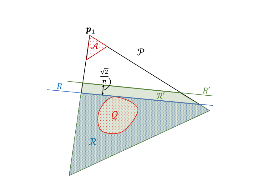
Figure 1: Geometrical relations between ${\cal Q}$, ${\cal R}$, ${\cal R}^{\prime}$, and ${\cal A}$ inside the set ${\cal P}$. The blue line is the hyperplane $R\coloneqq\{\bm{p}\in{\cal P}:\bm{u}\cdot\bm{p}=0\}$, which is a boundary of ${\cal R}$. This boundary is shifted by $\sqrt{2}/n$ to form the hyperplane $R^{\prime}$ (the green line), which is a boundary of ${\cal R}^{\prime}$.

Geometrical relations between the sets ${\cal Q}$, ${\cal R}$, ${\cal R}^{\prime}$, and ${\cal A}$ are illustrated in Fig. 1. This theorem gives a Sanov-type bound [6, 7] even though the quantum state is prepared by an adversary. Since Sanov-type inequalities are in general tighter than Azuma-Hoeffding-type inequalities [1, 5], which can also be applied in this setup, it may be useful in, for example, finite-size analyses of quantum cryptography. Note that Theorem 3 also holds for a classical probability mass function ${\cal M}^{n}$ instead of ${\cal M}^{\otimes n}(\rho)$ as long as all the conditional probability mass function of ${\cal M}^{n}$ conditioned on $n-1$ outcomes are contained in a set ${\cal Q}\subseteq{\cal P}$, which replaces the precondition Eq. (44) in this case.

I.3 Organization of the paper

In Sec. II, we prove Theorems 1–3 stated above, where each subsection is assigned for each theorem. In Sec. III, we apply our results to simple examples and numerically demonstrate the tightness of our bounds by comparison with conventionally used bounds. The first example in Sec. III.1 is an estimation task of measurement outcomes with two non-orthogonal projections, which is not directly related to real applications but is still informative. The second example is an application to the quantum key distribution protocol. Finally, in Sec. IV, we summarize our results and discuss possible applications.

II Proofs of the main theorems

II.1 A permutation-invariant quantum state is bounded by a mixture of i.i.d. quantum states

In this section, we develop a method to apply a concentration inequality for an independent and identically distributed (i.i.d.) state to a permutation-invariant state. The idea is to find an upper bound of a density operator of a permutation-invariant state with density operators of i.i.d. states up to a multiplication factor. This has been intensively studied in the context of the quantum de Finetti theorem (see e.g. [12] for a review) under the name of post-selection technique [9, 10, 11]. Here, we develop a refinement of the bound.

As defined prior to Theorem 1, let ${\cal H}_{A}$ be a $d$-dimensional Hilbert space, $Y_{n}^{d}$ be the set of Young diagrams with $n$ boxes and at most $d$ rows whose elements can be labeled by $\bm{n}=(n_{1},n_{2},\ldots,n_{d})$ with $n_{1}\geq n_{2}\geq\cdots n_{d}$ and $\sum_{i=1}^{d}n_{i}=n$. As shown in Eq. (2), ${\cal H}_{A}^{\otimes n}$ can be decomposed into the direct sum of the subspaces in the form ${\cal U}_{\bm{n}}\otimes{\cal V}_{\bm{n}}$ labeled by $\bm{n}\in Y_{n}^{d}$. Let $P_{\bm{n}}$ be a projection operator onto this subspace. Let $\rho_{A^{n}E}$ be a state on ${\cal H}_{A}^{\otimes n}\otimes{\cal H}_{E}$ that is invariant under the permutation of $n$ local systems of $A^{n}$. Then, from Schur’s lemma, $\rho_{A^{n}E}$ has the form

$$\rho_{A^{n}E}=\bigoplus_{\bm{n}\in Y_{n}^{d}}\mathrm{Tr}[P_{\bm{n}}\rho_{A^{n}E}]\,\rho_{{\cal U}_{\bm{n}}E}\otimes\frac{I_{{\cal V}_{\bm{n}}}}{\dim{\cal V}_{\bm{n}}},$$ (48)

where $\rho_{{\cal U}_{\bm{n}}E}$ denotes a density operator on the subspace ${\cal U}_{\bm{n}}$ and $E$, and $I_{{\cal V}_{\bm{n}}}$ is an identity operator on the subspace ${\cal V}_{\bm{n}}$. From this, it is obvious that the state $\rho_{A^{n}E}$ satisfies Eq. (3). We define a CPTP map ${\cal S}_{A^{n}}$ as follows:

$$\begin{split}{\cal S}_{A^{n}}(\tau_{A^{n}})&=\bigoplus_{\bm{n}\in Y_{n}^{d}}\bigl{(}\mathrm{Id}_{{\cal U}_{\bm{n}}}\otimes\mathrm{Tr}_{{\cal V}_{\bm{n}}}(P_{\bm{n}}\tau_{A^{n}}P_{\bm{n}}|_{{\cal U}_{\bm{n}}\otimes{\cal V}_{\bm{n}}})\bigr{)}\\ &\hskip 113.81102pt\otimes\ket{0}\!\bra{0}_{{\cal V}_{\bm{n}}},\end{split}$$ (49)

where $\ket{0}\!\bra{0}_{{\cal V}_{\bm{n}}}$ is an arbitrary pure state on ${\cal V}_{\bm{n}}$. From the definition, Eq. (6) in Theorem 1 obviously holds. We also define another CPTP map ${\cal R}_{A^{n}}$ as follows:

$$\begin{split}{\cal R}_{A^{n}}(\tau_{A^{n}})&=\bigoplus_{\bm{n}\in Y_{n}^{d}}\bigl{(}\mathrm{Id}_{{\cal U}_{\bm{n}}}\otimes\mathrm{Tr}_{{\cal V}_{\bm{n}}}(P_{\bm{n}}\tau_{A^{n}}P_{\bm{n}}|_{{\cal U}_{\bm{n}}\otimes{\cal V}_{\bm{n}}})\bigr{)}\\ &\hskip 113.81102pt\otimes\frac{I_{{\cal V}_{\bm{n}}}}{\dim{\cal V}_{\bm{n}}}.\end{split}$$ (50)

Then, it is obvious from Eq. (48) and the above that the CPTP maps ${\cal S}_{A^{n}}$ and ${\cal R}_{A^{n}}$ satisfy Eq. (7) in Theorem 1.

Now, let $\mathrm{diag}(\bm{t})$ be a density operator represented by a diagonal matrix with the spectrum $\bm{t}=(t_{1},\ldots,t_{d})$ in a fixed basis of ${\cal H}_{A}$. Without loss of generality, we assume $t_{1}\geq\cdots\geq t_{d}(\geq 0)$. Then, it is known that [13, 14, 15]

$$\mathrm{Tr}[P_{\bm{n}}\mathrm{diag}(\bm{t})^{\otimes n}]=\dim{\cal V}_{\bm{n}}\;s_{\bm{n}}(\bm{t}),$$ (51)

where $s_{\bm{n}}$ is the Schur function defined in Eq. (4). An alternative expression for the Schur function $s_{\bm{n}}(\bm{t})$ is given as follows. Let $T_{\bm{n}}$ be the set of semistandard Young tableaux of shape $\bm{n}$, i.e., Young diagrams filled with integers from $1$ to $d$ non-decreasingly across each row and increasingly down each column. Then, we have [13, 14]

$$s_{\bm{n}}(\bm{t})=\sum_{T_{\bm{n}}}t_{1}^{w_{1}}\cdots t_{d}^{w_{d}},$$ (52)

where $w_{i}$, $i=1,\ldots,d$, denotes the weight of a given Young tableau, i.e., the occurrences of the number $i$ in the Young tableau. Note that we define $0^{0}=1$ here. The largest element in the above summation is given by filling $i$-th row with $i$, which then implies

$$s_{\bm{n}}(\bm{t})\geq t_{1}^{n_{1}}\cdots t_{d}^{n_{d}}=\Pi_{i=1}^{n}t_{i}^{n_{i}}.$$ (53)

Now, let us consider, instead of $\mathrm{diag}(\bm{t})^{\otimes n}$ in Eq. (51), the state $\mathbb{E}_{U_{A}\sim\text{Haar}(d)}[(U_{A}\mathrm{diag}(\bm{t})U_{A}^{\dagger})^{\otimes n}]$, where $\mathbb{E}_{U\sim\text{Haar}(d)}[\cdot]$ denotes the Haar average over the $d$-dimensional unitary group $\mathrm{U}(d)$. This state commutes with any unitary in the form $U^{\prime\otimes n}$, $(U^{\prime}\in\mathrm{U}(d))$, as well as any permutation of the systems, and thus satisfies

$$P_{\bm{n}}\mathbb{E}_{U_{A}\sim\text{Haar}(d)}[(U_{A}\mathrm{diag}(\bm{t})U_{A}^{\dagger})^{\otimes n}]P_{\bm{n}}=\alpha_{\bm{n}}(\bm{t})P_{\bm{n}},$$ (54)

for coefficients $\alpha_{\bm{n}}(\bm{t})$ satisfying $\sum_{\bm{n}\in Y_{n}^{d}}\alpha_{\bm{n}}(\bm{t})=1$. (This is because $U^{\prime\otimes n}$ acts as $\pi_{\bm{n}}(U^{\prime})\otimes I_{{\cal V}_{\bm{n}}}$ on ${\cal U}_{\bm{n}}\otimes{\cal V}_{\bm{n}}$, where $\pi_{\bm{n}}$ is an irreducible representation of $\mathrm{U}(d)$ labeled by $\bm{n}$.) By taking the trace of both sides, we have

$$\begin{split}&\mathrm{Tr}\!\left[P_{\bm{n}}\mathbb{E}_{U_{A}\sim\text{Haar}(d)}\Bigl{[}\bigl{(}U_{A}\mathrm{diag}(\bm{t})U_{A}^{\dagger}\bigr{)}^{\otimes n}\Bigr{]}\right]\\ &=\alpha_{\bm{n}}(\bm{t})\dim({\cal U}_{\bm{n}}\otimes{\cal V}_{\bm{n}}).\end{split}$$ (55)

Since a unitary does not change the spectra, we have

$$\mathrm{Tr}\!\left(P_{\bm{n}}\mathbb{E}_{U_{A}\sim\text{Haar}(d)}[(U_{A}\mathrm{diag}(\bm{t})U_{A}^{\dagger})^{\otimes n}]\right)$$

$$=\mathbb{E}_{U_{A}\sim\text{Haar}(d)}\left[\mathrm{Tr}(P_{\bm{n}}(U_{A}\mathrm{diag}(\bm{t})U_{A}^{\dagger})^{\otimes n})\right]$$ (56)

$$=\mathbb{E}_{U_{A}\sim\text{Haar}(d)}[\dim{\cal V}_{\bm{n}}\;s_{\bm{n}}(\bm{t})]$$ (57)

$$=\dim{\cal V}_{\bm{n}}\;s_{\bm{n}}(\bm{t}).$$ (58)

Therefore, from Eqs. (55) and (58), we have

$$\alpha_{\bm{n}}(\bm{t})=\frac{s_{\bm{n}}(\bm{t})}{\dim{\cal U}_{\bm{n}}}.$$ (59)

Now, from Eqs. (48) and (49), we have

$$\begin{split}&\mathrm{supp}({\cal S}_{A^{n}}(P_{\bm{n}}\rho_{A^{n}}P_{\bm{n}}))\\ &=\begin{cases}\mathrm{supp}(\rho_{{\cal U}_{\bm{n}}})\otimes\ket{0}\!\bra{0}_{{\cal V}_{\bm{n}}}&\text{on }{\cal U}_{\bm{n}}\otimes{\cal V}_{\bm{n}}\\ 0&\text{otherwise}\end{cases}.\end{split}$$ (60)

Combining the above with Eqs.(49), (54), and (59), we have

$$\mathrm{supp}({\cal S}_{A^{n}}(P_{\bm{n}}\rho_{A^{n}}P_{\bm{n}}))$$

$$\leq\frac{{\cal S}_{A^{n}}(P_{\bm{n}})}{\dim{\cal V}_{\bm{n}}}$$ (61)

$$=\frac{1}{\alpha_{\bm{n}}(\bm{t})\dim{\cal V}_{\bm{n}}}{\cal S}_{A^{n}}(P_{\bm{n}}\mathbb{E}_{U_{A}\sim\text{Haar}(d)}[(U_{A}\mathrm{diag}(\bm{t})U_{A}^{\dagger})^{\otimes n}]P_{\bm{n}})$$ (62)

$$\leq\frac{\dim{\cal U}_{\bm{n}}}{s_{\bm{n}}(\bm{t})\dim{\cal V}_{\bm{n}}}{\cal S}_{A^{n}}(\mathbb{E}_{U_{A}\sim\text{Haar}(d)}[(U_{A}\mathrm{diag}(\bm{t})U_{A}^{\dagger})^{\otimes n}])$$ (63)

We thus obtain the following from Eqs. (49), (50), and (63).

Lemma 1.

Consider a composite system $A^{n}E$ associated with a Hilbert space ${\cal H}_{A}^{n}\otimes{\cal H}_{E}$ with $\dim{\cal H}_{A}=d$. Then, there exists a pair $({\cal S}_{A^{n}},{\cal R}_{A^{n}})$ of CPTP maps that satisfies the following conditions (i) and (ii).

(i) For any $\rho_{A^{n}E}$ that is invariant under permutation of $n$ subsystems of $A^{n}$, the pair $({\cal S}_{A^{n}},{\cal R}_{A^{n}})$ satisfies

$${\cal R}_{A^{n}}\circ{\cal S}_{A^{n}}\otimes\mathrm{Id}_{E}(\rho_{A^{n}E})=\rho_{A^{n}E}.$$ (64)

(ii) For any $\rho_{A^{n}}$ that is invariant under permutation of $n$ subsystems of $A^{n}$ and for any $\bm{n}\in Y_{n}^{d}$ and $\bm{t}=(t_{1},\ldots,t_{d})$ with $t_{i}\geq 0$ and $\sum_{i=1}^{d}t_{i}=1$, we have

$$\mathrm{supp}({\cal S}_{A^{n}}(P_{\bm{n}}\rho_{A^{n}}P_{\bm{n}}))$$

$$\leq\frac{\dim{\cal U}_{\bm{n}}}{s_{\bm{n}}(\bm{t})\dim{\cal V}_{\bm{n}}}{\cal S}_{A^{n}}\!\Bigl{(}\mathbb{E}_{U_{A}\sim{\rm Haar}(d)}\Bigl{[}\bigl{(}U_{A}\,\mathrm{diag}(\bm{t})\,U_{A}^{\dagger}\bigr{)}^{\otimes n}\Bigr{]}\Bigr{)}$$ (65)

By setting $\bm{t}=\bm{n}/n$ in Lemma 1, we proved Theorem 1 except for Eqs. (9) and (10). In fact, the choice $\bm{t}=\bm{n}/n$ is almost optimal to obtain the smallest coefficient in the right-hand side of Eq. (65), which we explain in the following. First, it is known that the dimension of ${\cal V}_{\bm{n}}$ can be represented as [13, 14]

$$\dim{\cal V}_{\bm{n}}=\frac{n!}{\prod_{(i,j)}h_{\bm{n}}(i,j)},$$ (66)

where $h_{\bm{n}}(i,j)$ denotes the hook length of the Young diagram at $(i,j)$, i.e., $i$-th row and $j$-th column. On the other hand, the dimension of ${\cal U}_{\bm{n}}$ is given by [13, 14]

$$\dim{\cal U}_{\bm{n}}=\prod_{(i,j)}\frac{d-i+j}{h_{\bm{n}}(i,j)},$$ (67)

and therefore,

$$\frac{\dim{\cal U}_{\bm{n}}}{\dim{\cal V}_{\bm{n}}}=\prod_{(i,j)}\frac{d-i+j}{n!}=\frac{n_{1}!\ldots n_{d}!}{n!}\prod_{i=1}^{d}{d-i+n_{i}\choose d-i},$$ (68)

which holds even when $n_{j}=\cdots=n_{d}=0$ for $1\leq j\leq d$. Combining this with Eq. (53), we have

$$\frac{\dim{\cal U}_{\bm{n}}}{\dim{\cal V}_{\bm{n}}\;s_{\bm{n}}(\bm{t})}\leq\frac{1}{\mathrm{Mult}_{\bm{t}}(\bm{n})}\prod_{i=0}^{d-1}{n+i\choose i},$$ (69)

where $\mathrm{Mult}_{\bm{t}}$ denotes the probability density function (PDF) of the multinomial distribution with the probability vector $\bm{t}$. Now, it is clear that the choice $\bm{t}=\bm{n}/n$ maximizes $\mathrm{Mult}_{\bm{t}}(\bm{n})$, which is bounded from below as

$$\mathrm{Mult}_{\bm{n}/n}(\bm{n}) =\frac{n!}{n_{1}!\cdots n_{d}!}\left(\frac{n_{1}}{n}\right)^{n_{1}}\cdots\left(\frac{n_{d}}{n}\right)^{n_{d}}$$ (70)

$$\geq\frac{\sqrt{2\pi n}}{e^{d}\sqrt{n_{1}\cdots n_{d}}}$$ (71)

$$\geq\bigl{(}2\pi(d/e^{2})^{d}n^{-(d-1)}\bigr{)}^{\frac{1}{2}},$$ (72)

where we used Stirling’s inequality in the first inequality and used the relation between the arithmetic mean and the geometric mean in the second inequality. We thus have

$$\frac{\dim{\cal U}_{\bm{n}}}{\dim{\cal V}_{\bm{n}}\;s_{\bm{n}}(\bm{n}/n)}$$

$$\leq\bigl{(}2\pi(d/e^{2})^{d}n^{-(d-1)}\bigr{)}^{-\frac{1}{2}}\prod_{i=0}^{d-1}{n+i\choose i}$$ (73)

$$\leq\frac{n^{\frac{d-1}{2}}}{\sqrt{2\pi(d/e^{2})^{d}}}\prod_{i=0}^{d-1}\frac{(n+d-1)^{i}}{i!}$$ (74)

$$\leq\frac{(n+d-1)^{\frac{(d^{2}-1)}{2}}}{\sqrt{2\pi(d/e^{2})^{d}}G(d+1)}=f_{q}(n,d),$$ (75)

where $G(n)$ denotes the Barnes G-function defined in Eq. (5). Notice that we used the following trivial inequalities from Eq. (73) to Eq. (74)

$${n+i\choose i}=\overbrace{\frac{(n+i)\cdots(n+1)}{i!}}^{i}\leq(n+d-1)^{i}/i!.$$ (76)

(Note: the bound ${n+i\choose i}\leq(n+1)^{i}$ is conventionally used for this context, but this leads to a looser bound in the case $n\gg d$, which is of our interest.) This proves Eqs. (9) and (10) in Theorem 1, which completes the proof of Theorem 1 combined with Lemma 1.∎

Theorem 1 may have lots of applications. One immediate example is the following. Assume that a positive operator $\Pi$ satisfies $\mathrm{Tr}(\Pi\rho^{\otimes n})\leq\mathcal{O}(\exp(-n))$ for any $\rho$. Such a positive operator $\Pi$ frequently appears in a quantum key distribution or a quantum state verification. For such a scenario, we have, for any permutation-invariant state $\rho_{A^{n}}$,

$$\begin{split}\mathrm{Tr}[\Pi\rho_{A^{n}}]&\leq f_{q}(n,d)\sum_{\bm{n}\in Y_{n}^{d}}\mathrm{Tr}[P_{\bm{n}}\rho_{A^{n}}]\\ &\quad\times\mathrm{Tr}\!\left(\Pi\,\mathbb{E}_{U\sim\text{Haar}(d)}[(U\mathrm{diag}(\bm{n}/n)U^{\dagger})^{\otimes n}]\right),\end{split}$$ (77)

$$\leq f_{q}(n,d)\sum_{\bm{n}\in Y_{n}^{d}}\mathrm{Tr}[P_{\bm{n}}\rho_{A^{n}}]\,\sup_{\rho}\mathrm{Tr}(\Pi\rho^{\otimes n}),$$ (78)

$$\leq f_{q}(n,d)\mathcal{O}(\exp(-n)),$$ (79)

and thus almost the same exponential bound holds (up to a polynomial $f_{q}(n,d)$). The above inequality will be used later.

II.2 Generalization to the case with symmetry restrictions

In this section, we generalize the result of the previous section to the case in which a local $d$-dimensional system has an additional symmetry. There are lots of relevant situations in quantum information applications in which a local system has a symmetry. A classical-quantum state, for example, can be regarded as a quantum state having a $\mathrm{U}(1)$ symmetry in a part of a system. To make it more concrete, we here derive a tighter upper bound on a permutation-invariant state by i.i.d. states when a local system has an additional symmetry. Let $G$ be a group that acts as a symmetry of local system $A$ whose Hilbert space is ${\cal H}_{A}$. Then, without loss of generality, ${\cal H}_{A}$ can be decomposed into the direct sum given in Eq. (19) on which the representation $\pi$ of the group $G$ acts as in Eq. (20). Any state $\rho_{AE}^{G}$ that is invariant under the action of the group $G$ on the system $A$ should have the form

$$\rho_{AE}^{G}=\bigoplus_{j=1}^{k}\mathrm{Tr}(Q_{j}\rho^{G})\frac{I_{{\cal H}_{j}^{R}}}{r_{j}}\otimes\rho_{{\cal H}_{j}^{D}E},$$ (80)

with a set of density operators $\{\rho_{{\cal H}_{j}^{D}E}\}_{j=1}^{k}$, where $Q_{j}$ denotes the projection onto the subspace ${\cal H}_{j}^{R}\otimes{\cal H}_{j}^{D}$. Let $(s_{A},r_{A})$ be a pair of CPTP maps defined as follows:

$$\begin{split}s_{A}(\tau_{A})&=\bigoplus_{j=1}^{k}\ket{\varnothing_{j}}\!\bra{\varnothing_{j}}_{{\cal H}_{j}^{R}}\\ &\hskip 28.45274pt\otimes(\mathrm{Tr}_{{\cal H}_{j}^{R}}\otimes\mathrm{Id}_{{\cal H}_{j}^{D}})(Q_{j}\tau_{A}Q_{j}|_{{\cal H}_{j}^{R}\otimes{\cal H}_{j}^{D}}),\end{split}$$ (81)

$$r_{A}(\tau_{A}) =\bigoplus_{j=1}^{k}\frac{I_{{\cal H}_{j}^{R}}}{r_{j}}\otimes(\mathrm{Tr}_{{\cal H}_{j}^{R}}\otimes\mathrm{Id}_{{\cal H}_{j}^{D}})(Q_{j}\tau_{A}Q_{j}|_{{\cal H}_{j}^{R}\otimes{\cal H}_{j}^{D}}),$$ (82)

where $\ket{\varnothing_{j}}\!\bra{\varnothing_{j}}_{{\cal H}_{j}^{R}}$ denotes arbitrary pure states on ${\cal H}_{j}^{R}$. Then, we have

$$r_{A}\circ s_{A}\otimes\mathrm{Id}_{E}(\rho_{AE}^{G})=\rho_{AE}^{G}.$$ (83)

Since each local system has this direct-sum structure for a $G$-invariant state, $\pi^{\otimes n}(G^{\times n})$-invariant state ${\rho}_{A^{n}E}^{G}$ also has this direct-sum structure locally, which we want to exploit first. Let us define a sequence $\bm{j}\coloneqq(j_{1},\ldots,j_{n})\in\{1,\ldots,k\}^{\times n}$. This sequence corresponds one-to-one to the direct summand of $\rho_{A^{n}E}^{G}$ on the subspace ${\cal H}_{\bm{j}}$ defined in Eq. (23). Let $Q_{\bm{j}}$ be a projection operator onto this subspace, i.e.,

$$Q_{\bm{j}}=Q_{j_{1}}\otimes\cdots\otimes Q_{j_{n}},$$ (84)

where $Q_{\bm{j}}Q_{\bm{j}^{\prime}}=\delta_{\bm{j}\bm{j}^{\prime}}$. Furthermore, let $Z_{n}^{k}$ be as defined prior to Theorem 2. Then,

$${\rho}_{A^{n}E}^{G}=\sum_{\bm{j}\in\{1,\ldots,k\}^{\times n}}Q_{\bm{j}}{\rho}_{A^{n}E}^{G}Q_{\bm{j}}=\sum_{\bm{m}\in Z_{n}^{k}}\sum_{\bm{j}\in{\cal T}(\bm{m})}Q_{\bm{j}}{\rho}_{A^{n}E}^{G}Q_{\bm{j}},$$ (85)

where ${\cal T}(\bm{m})$ is as defined in Eq. (25). The cardinality of this set ${\cal T}(\bm{m})$ is given by

$$|{\cal T}(\bm{m})|=\frac{n!}{n_{1}!\cdots n_{k}!}.$$ (86)

For each $\bm{m}\in Z_{n}^{k}$, let us define

$$\bm{j}_{0}(\bm{m})=(\underbrace{1,\ldots,1}_{n_{1}},\underbrace{2,\ldots,2}_{n_{2}},\ldots,\underbrace{k,\ldots,k}_{n_{k}}).$$ (87)

Then, for any $\bm{j}\in{\cal T}(\bm{m})$, there exists a permutation $\sigma_{\bm{j}}\in S_{n}$ such that $\bm{j}=\sigma_{\bm{j}}(\bm{j}_{0}(\bm{m}))$. Thus, we can choose a subset $S^{\prime}\subseteq S_{n}$ with $|S^{\prime}|=|{\cal T}(\bm{m})|$ such that

$$S^{\prime}=\{\sigma_{\bm{j}}:\bm{j}\in{\cal T}(\bm{m}),\,\sigma_{\bm{j}}\bigl{(}\bm{j}_{0}(\bm{m})\bigr{)}=\bm{j}\}.$$ (88)

A choice of such $S^{\prime}$ is not unique, but the following arguments do not depend on the specific choice of $S^{\prime}$. Let $V_{\sigma}$ be a unitary representation of $\sigma\in S_{n}$ on ${\cal H}_{A}^{\otimes n}$. Then, for any $\bm{j}\in{\cal T}(\bm{m})$, there exists $\sigma_{\bm{j}}\in S^{\prime}$ such that the following holds:

$$Q_{\bm{j}}=V_{\sigma_{\bm{j}}}Q_{\bm{j}_{0}(\bm{m})}V_{\sigma_{\bm{j}}}^{\dagger}.$$ (89)

From Eq. (80), we have

$$\begin{split}&Q_{\bm{j}_{0}(\bm{m})}\,{\rho}_{A^{n}E}^{G}\,Q_{\bm{j}_{0}(\bm{m})}\\ &=\mathrm{Tr}[Q_{\bm{j}_{0}(\bm{m})}{\rho}_{A^{n}E}^{G}]\bigotimes_{j=1}^{k}\left(\frac{I_{{\cal H}_{j}^{R}}}{r_{j}}\right)^{\otimes n_{j}}\otimes\rho_{({\cal H}_{j}^{D})^{\otimes n_{j}}E},\end{split}$$ (90)

with a set of density operators $\{\rho_{({\cal H}_{j}^{D})^{\otimes n_{j}}E}\}_{j=1}^{k}$, and from Eq. (81), we have

$$s_{A}^{\otimes n}\otimes\mathrm{Id}_{E}(Q_{\bm{j}_{0}(\bm{m})}\,{\rho}_{A^{n}E}^{G}\,Q_{\bm{j}_{0}(\bm{m})})$$

$$=Q_{\bm{j}_{0}(\bm{m})}\,s_{A}^{\otimes n}\otimes\mathrm{Id}_{E}({\rho}_{A^{n}E}^{G})\,Q_{\bm{j}_{0}(\bm{m})}$$ (91)

$$=\mathrm{Tr}[Q_{\bm{j}_{0}(\bm{m})}{\rho}_{A^{n}E}^{G}]\bigotimes_{j=1}^{k}\ket{\varnothing_{j}}\!\bra{\varnothing_{j}}_{{\cal H}_{j}^{R}}^{\otimes n_{j}}\otimes\rho_{({\cal H}_{j}^{D})^{\otimes n_{j}}E}.$$ (92)

Now we exploit the permutation invariance of $\rho^{G}_{A^{n}E}$ in the $n$ local systems of $A^{n}$. Since $\ket{\varnothing_{j}}\!\bra{\varnothing_{j}}_{{\cal H}_{j}^{R}}^{\otimes n_{j}}\otimes\rho_{({\cal H}_{j}^{D})^{\otimes n_{j}}E}$ is invariant under the (joint) permutation of $({\cal H}_{j}^{R}\otimes{\cal H}_{j}^{D})^{\otimes n_{j}}$ for each $j=1,\ldots,k$, we can apply Theorem 1 and Eq. (3) to $(\ket{\varnothing_{j}}\!\bra{\varnothing_{j}}_{{\cal H}_{j}^{R}}\otimes{\cal H}_{j}^{D})^{\otimes n_{j}}$ for $j=1,\ldots,k$ to have

$$Q_{\bm{j}_{0}(\bm{m})}\,s_{A}^{\otimes n}\otimes\mathrm{Id}_{E}({\rho}_{A^{n}E}^{G})\,Q_{\bm{j}_{0}(\bm{m})}$$

$$\begin{split}&=\sum_{\begin{subarray}{c}(\bm{n}_{1},\ldots,\bm{n}_{k})\\ \in Y_{n_{1}}^{d_{1}}\times\cdots\times Y_{n_{k}}^{d_{k}}\end{subarray}}\\ &\quad P_{\bm{n}_{1}}\otimes\cdots\otimes P_{\bm{n}_{k}}\,s_{A}^{\otimes n}\otimes\mathrm{Id}_{E}({\rho}_{A^{n}E}^{G})\,P_{\bm{n}_{1}}\otimes\cdots\otimes P_{\bm{n}_{k}}\end{split},$$ (93)

where $P_{\bm{n}_{j}}$ denotes the projection operator onto the irreducible subspace $(\ket{\varnothing_{j}}\!\bra{\varnothing_{j}}_{{\cal H}_{j}^{R}})^{\otimes n_{j}}\otimes{\cal U}_{\bm{n}_{j}}\otimes{\cal V}_{\bm{n}_{j}}$ of $(\ket{\varnothing_{j}}\!\bra{\varnothing_{j}}_{{\cal H}_{j}^{R}}\otimes{\cal H}_{j}^{D})^{\otimes n_{j}}$ with the Young diagram $\bm{n}_{j}\in Y_{n_{j}}^{d_{j}}$. Note, for $P_{\bm{n}_{j}}$, we have

$$\sum_{\bm{n}_{j}\in Y_{n_{j}}^{d_{j}}}P_{\bm{n}_{j}}=(\ket{\varnothing_{j}}\!\bra{\varnothing_{j}}_{{\cal H}_{j}^{R}}\otimes I_{{\cal H}_{j}^{D}})^{\otimes n_{j}}\leq Q_{\bm{j}_{0}(\bm{m})},$$ (94)

and also have

$$\begin{split}&s_{A}^{\otimes n}\otimes\mathrm{Id}_{E}(P_{\bm{m};\bm{n}_{1},\ldots,\bm{n}_{k}}{\rho}_{A^{n}E}^{G}P_{\bm{m};\bm{n}_{1},\ldots,\bm{n}_{k}})\\ &=\sum_{\bm{j}\in{\cal T}(\bm{m})}V_{\sigma_{\bm{j}}}P_{\bm{n}_{1}}\otimes\cdots\otimes P_{\bm{n}_{k}}\\ &\qquad\qquad\quad s_{A}^{\otimes n}\otimes\mathrm{Id}_{E}({\rho}_{A^{n}E}^{G})\,P_{\bm{n}_{1}}\otimes\cdots\otimes P_{\bm{n}_{k}}V_{\sigma_{\bm{j}}}^{\dagger},\end{split}$$ (95)

where $P_{\bm{m};\bm{n}_{1},\ldots,\bm{n}_{k}}$ is as defined prior to Theorem 2. Combining the above with Eqs. (83), (85), (89), (91), and (93), we have Eq. (34) in Theorem 2. Furthermore, since any output state of $s_{A}^{\otimes n}$ has the form $\ket{\varnothing_{j}}\!\bra{\varnothing_{j}}^{\otimes n}$ on $({\cal H}_{j}^{R})^{\otimes n}$, we have

$$\begin{split}&\sum_{\bm{j}\in{\cal T}(\bm{m})}V_{\sigma_{\bm{j}}}P_{\bm{n}_{1}}\otimes\cdots\otimes P_{\bm{n}_{k}}\\ &\qquad\qquad\quad s_{A}^{\otimes n}\otimes\mathrm{Id}_{E}({\rho}^{G}_{A^{n}E})\,P_{\bm{n}_{1}}\otimes\cdots\otimes P_{\bm{n}_{k}}V_{\sigma_{\bm{j}}}^{\dagger}\\ &=P_{\bm{m};\bm{n}_{1},\ldots,\bm{n}_{k}}s_{A}^{\otimes n}\otimes\mathrm{Id}_{E}({\rho}^{G}_{A^{n}E})P_{\bm{m};\bm{n}_{1},\ldots,\bm{n}_{k}}.\end{split}$$ (96)

For $\bm{m}\in Z_{n}^{k}$, we define $\tilde{S}_{A^{n}}[\bm{m}]$ and $\tilde{R}_{A^{n}}[\bm{m}]$ as

$$\begin{split}&\tilde{S}_{A^{n}}[\bm{m}](\rho_{A^{n}})\\ &\coloneqq\bigotimes_{j=1}^{k}{\cal S}_{(\ket{\varnothing_{j}}\!\bra{\varnothing_{j}}_{{\cal H}_{j}^{R}}\otimes{\cal H}_{j}^{D})^{\otimes n_{j}}}\biggl{(}\sum_{\bm{j}\in{\cal T}(\bm{m})}V_{\sigma_{\bm{j}}}^{\dagger}Q_{\bm{j}}\rho_{A^{n}}Q_{\bm{j}}V_{\sigma_{\bm{j}}}\biggr{)},\end{split}$$ (97)

$$\begin{split}&\tilde{R}_{A^{n}}[\bm{m}](\rho_{A^{n}})\\ &\coloneqq\sum_{\bm{j}\in{\cal T}(\bm{m})}Q_{\bm{j}}V_{\sigma_{\bm{j}}}\biggl{[}\bigotimes_{j=1}^{k}{\cal R}_{(\ket{\varnothing_{j}}\!\bra{\varnothing_{j}}_{{\cal H}_{j}^{R}}\otimes{\cal H}_{j}^{D})^{\otimes n_{j}}}\bigl{(}\rho_{A^{n}}\bigr{)}\biggr{]}V_{\sigma_{\bm{j}}}^{\dagger}Q_{\bm{j}}.\end{split}$$ (98)

By definition, these maps are trace non-increasing. From Eqs. (7), (85), (89), and (92), we have

$$\tilde{\cal S}_{A^{n}}[\bm{m}](\rho_{A^{n}}) =Q_{\bm{j}_{0}(\bm{m})}\tilde{\cal S}_{A^{n}}[\bm{m}](\rho_{A^{n}})Q_{\bm{j}_{0}(\bm{m})},$$ (99)

$$=\tilde{\cal S}_{A^{n}}[\bm{m}]\biggl{(}\sum_{\bm{j}\in{\cal T}(\bm{m})}Q_{\bm{j}}\rho_{A^{n}}Q_{\bm{j}}\biggr{)}$$ (100)

and

$$\begin{split}&\tilde{\cal R}_{A^{n}}[\bm{m}]\circ\tilde{\cal S}_{A^{n}}[\bm{m}]\otimes\mathrm{Id}_{E}\bigl{(}s_{A}^{\otimes n}\otimes\mathrm{Id}_{E}({\rho}_{A^{n}E}^{G})\bigr{)}\\ &=\sum_{\bm{j}\in{\cal T}(\bm{m})}Q_{\bm{j}}s_{A}^{\otimes n}\otimes\mathrm{Id}_{E}({\rho}_{A^{n}E}^{G})Q_{\bm{j}}.\end{split}$$ (101)

Furthermore, from Eqs. (6) and (18), for any $\bm{m}\in Z_{n}^{k}$ and any $(\bm{n}_{1},\ldots,\bm{n}_{k})\in Y_{n}^{1}\times\cdots\times Y_{n}^{k}$, we have

$$\mathrm{supp}\!\left(P_{\bm{n}_{1}}\otimes\cdots\otimes P_{\bm{n}_{k}}\,\tilde{S}_{A^{n}}[\bm{m}]\bigl{(}s_{A}^{\otimes n}({\rho}_{A^{n}}^{G})\bigr{)}\,P_{\bm{n}_{1}}\otimes\cdots\otimes P_{\bm{n}_{k}}\right)$$

$$\begin{split}&\leq\bigotimes_{j=1}^{k}f_{q}(n_{j},d_{j}){\cal S}_{(\ket{\varnothing_{j}}\!\bra{\varnothing_{j}}_{{\cal H}_{j}^{R}}\otimes{\cal H}_{j}^{D})^{\otimes n_{j}}}\biggl{(}\ket{\varnothing_{j}}\!\bra{\varnothing_{j}}_{{\cal H}_{j}^{R}}^{\otimes n_{j}}\\ &\qquad\quad\otimes\mathbb{E}_{U_{j}^{D}\sim\mathrm{Haar}(d_{j})}\Bigl{[}\Bigl{(}U_{j}^{D}\mathrm{diag}\Bigl{(}\frac{\bm{n}_{j}}{n_{j}}\Bigr{)}(U_{j}^{D})^{\dagger}\Bigr{)}_{{\cal H}_{j}^{D}}^{\otimes n_{j}}\Bigr{]}\biggr{)}.\end{split}$$ (102)

Unfortunately, the right-hand side of the above is still not an i.i.d. state. Thus, we further need to find an upper bound on the right-hand side above. For that, let $\bm{U}\coloneqq(U_{1}^{D},\ldots,U_{k}^{D})$ and define the following density operator on the system $A$:

$$\tau_{\bm{U}}(\bm{n}_{1},\ldots,\bm{n}_{k})=\bigoplus_{j=1}^{k}\frac{I_{{\cal H}_{j}^{R}}}{r_{j}}\otimes\Bigl{(}U_{j}^{D}\mathrm{diag}\Bigl{(}\frac{\bm{n}_{j}}{n}\Bigr{)}(U_{j}^{D})^{\dagger}\Bigr{)}_{{\cal H}_{j}^{D}},$$ (103)

and consider $\sum_{\bm{j}\in{\cal T}(\bm{m})}V_{\sigma_{\bm{j}}}^{\dagger}Q_{\bm{j}}s_{A}^{\otimes n}(\tau_{\bm{U}}(\bm{n}_{1},\ldots,\bm{n}_{k}))Q_{\bm{j}}V_{\sigma_{\bm{j}}}$. From Eqs. (81) and (97), we have

$$\begin{split}&\sum_{\bm{j}\in{\cal T}(\bm{m})}V_{\sigma_{\bm{j}}}^{\dagger}Q_{\bm{j}}s_{A}^{\otimes n}(\tau_{\bm{U}}(\bm{n}_{1},\ldots,\bm{n}_{k}))Q_{\bm{j}}V_{\sigma_{\bm{j}}}\\ &=|{\cal T}(\bm{m})|\bigotimes_{j=1}^{k}\biggl{(}\ket{\varnothing_{j}}\!\bra{\varnothing_{j}}_{{\cal H}_{j}^{R}}^{\otimes n_{j}}\\ &\qquad\quad\otimes\mathbb{E}_{U_{j}^{D}\sim\mathrm{Haar}(d_{j})}\Bigl{[}\Bigl{(}U_{j}^{D}\mathrm{diag}\Bigl{(}\frac{\bm{n}_{j}}{n}\Bigr{)}(U_{j}^{D})^{\dagger}\Bigr{)}_{{\cal H}_{j}^{D}}^{\otimes n_{j}}\Bigr{]}\biggr{)}\end{split}$$ (104)

$$\begin{split}&=\mathrm{Mult}_{\bm{m}/n}(\bm{m})\bigotimes_{j=1}^{k}\biggl{(}\ket{\varnothing_{j}}\!\bra{\varnothing_{j}}_{{\cal H}_{j}^{R}}^{\otimes n_{j}}\\ &\qquad\quad\otimes\mathbb{E}_{U_{j}^{D}\sim\mathrm{Haar}(d_{j})}\Bigl{[}\Bigl{(}U_{j}^{D}\mathrm{diag}\Bigl{(}\frac{\bm{n}_{j}}{n_{j}}\Bigr{)}(U_{j}^{D})^{\dagger}\Bigr{)}_{{\cal H}_{j}^{D}}^{\otimes n_{j}}\Bigr{]}\biggr{)}\end{split},$$ (105)

where we used Eq. (86) and the definition of the multinomial distribution $\mathrm{Mult}_{\bm{t}}$ in Eq. (70) in the last equality. From Eqs. (39) and (72), we have

$$\mathrm{Mult}_{\bm{m}/n}(\bm{m})\geq\bigl{(}f_{c}(n,k)\bigr{)}^{-1}$$ (106)

Then, from the above and Eqs. (97) and (102), we have

$$\mathrm{supp}\!\left(P_{\bm{n}_{1}}\otimes\cdots\otimes P_{\bm{n}_{k}}\tilde{S}_{A^{n}}\![\bm{m}]\bigl{(}s_{A}^{\otimes n}({\rho}_{A^{n}}^{G})\bigr{)}P_{\bm{n}_{1}}\otimes\cdots\otimes P_{\bm{n}_{k}}\right)$$

$$\begin{split}&\leq f_{c}(n,k)\prod_{j=1}^{k}f_{q}(n_{j},d_{j})\\ &\qquad\tilde{S}_{A^{n}}\![\bm{m}]\Bigl{(}s_{A}^{\otimes n}\bigl{(}\mathbb{E}_{\bm{U}\sim\bigtimes_{j=1}^{k}\mathrm{Haar}(d_{j})}[\tau_{\bm{U}}(\bm{n}_{1},\ldots,\bm{n}_{k})]\bigr{)}\Bigr{)}.\end{split}$$ (107)

Now, we define a pair $({\cal S}^{G}_{A^{n}},{\cal R}^{G}_{A^{n}})$ of CPTP maps as follows:

$${\cal S}^{G}_{A^{n}} \coloneqq\sum_{\bm{m}\in Z_{n}^{k}}\tilde{S}_{A^{n}}[\bm{m}]\circ s_{A}^{\otimes n},$$ (108)

$${\cal R}^{G}_{A^{n}} \coloneqq\sum_{\bm{m}\in Z_{n}^{k}}r_{A}^{\otimes n}\circ\tilde{R}_{A^{n}}[\bm{m}].$$ (109)

These maps are actually TP from Eqs. (84), (100), and (101). From Eqs. (83), (85), and (101), we have

$${\cal R}^{G}_{A^{n}}\circ{\cal S}^{G}_{A^{n}}\otimes\mathrm{Id}_{E}({\rho}_{A^{n}E}^{G})={\rho}_{A^{n}E}^{G},$$ (110)

which proves Eq. (37) in Theorem 2. Furthermore, from Eqs. (6), (95), (96), (97), and (108) with the fact that $\sum_{\bm{j}\in{\cal T}(\bm{m})}V_{\sigma_{\bm{j}}}^{\dagger}Q_{\bm{j}}$ and $P_{\bm{m};\bm{n}_{1},\ldots,\bm{n}_{k}}$ commute, we have Eq. (36) in Theorem 2. Finally, from Eqs. (35), (95), and (107), we have

$$\mathrm{supp}\left({\cal S}^{G}_{A^{n}}\Bigl{(}\rho_{A^{n}}^{G}(\bm{m};\bm{n}_{1},\ldots,\bm{n}_{k})\Bigr{)}\right)$$

$$\begin{split}&\leq\mathrm{supp}\Bigl{(}P_{\bm{n}_{1}}\otimes\cdots\otimes P_{\bm{n}_{k}}\,{\cal S}^{G}_{A^{n}}\bigl{(}{\rho}_{A^{n}}^{G}\bigr{)}\,P_{\bm{n}_{1}}\otimes\cdots\otimes P_{\bm{n}_{k}}\Bigr{)}\end{split}$$ (111)

$$\begin{split}&\leq f_{c}(n,k)\prod_{j=1}^{k}f_{q}(n_{j},d_{j})\\ &\quad\times{\cal S}^{G}_{A^{n}}\!\left(\mathbb{E}_{\bm{U}\sim\bigtimes_{j=1}^{k}\mathrm{Haar}(d_{j})}\bigl{[}\tau_{\bm{U}}(\bm{n}_{1},\ldots,\bm{n}_{k})^{\otimes n}\bigr{]}\right),\end{split}$$ (112)

which proves Eq. (38) in Theorem 2, and thus completes the proof. ∎

A particularly interesting case is when $G=\mathrm{U}(1)$. Since all the irreducible representations of $\mathrm{U}(1)$ is one dimensional, $r_{j}=1$ for any $j$. Let us further assume that $d_{1}=\cdots=d_{k}=d/k$. This case can be regarded as a classical-quantum state with $k$ being the dimension of the classical system. Then, the coefficient would be

$$f_{c}(n,k)\prod_{j=1}^{k}f_{q}(n_{j},d_{j})\simeq\mathcal{O}\bigl{(}n^{\frac{d^{2}/k-1}{2}}\bigr{)},$$ (113)

and thus we have approximately power-of-$k$ improvement compared to the case when we would not consider the symmetry, i.e., when applying Theorem 1 naively.

II.3 Concentration inequality for an independent and identical measurement on an adversarial state

Now we leave from concentration inequality for a quantum state and consider a concentration inequality for quantum measurement outcomes. In this section, we consider the case where independent and identical measurements ${\cal M}^{\otimes n}$ are performed on an adversarial state $\rho$. Let ${\cal M}^{\otimes n}(\rho):{\cal X}^{\times n}\to[0,1]$ be a probability mass function as defined in Theorem 3, and let $\mathrm{P}_{\rho}:Z_{n}^{k}\to[0,1]$ be another probability mass function defined as

$$\mathrm{P}_{\rho}(\bm{m})\coloneqq\sum_{\bm{i}\in{\cal T}(\bm{m})}{\cal M}^{\otimes n}(\rho)(\bm{i}).$$ (114)

Since we will consider a concentration inequality for the empirical probability of the measurement outcomes, the relevant probability mass function is $\mathrm{P}_{\rho}(\bm{m})$ rather than ${\cal M}^{\otimes n}(\rho)$. Furthermore, since $\bm{m}$ is invariant under the permutation of measurement outcomes $\bm{i}$, we have

$$\mathrm{P}_{\rho}(\bm{m})=\mathrm{P}_{\tilde{\rho}}(\bm{m}),$$ (115)

where $\tilde{\rho}$ is the permutation-symmetrized version of $\rho$. Thus, we consider $\tilde{\rho}$ instead of $\rho$ in the following analysis. Due to the permutation invariance, we can apply Theorem 2 to ${\cal M}^{\otimes n}(\tilde{\rho})$ with $r_{j}=d_{j}=1$ for $j=1,\ldots,k$ and obtain

$${\cal M}^{\otimes n}(\tilde{\rho})(\bm{i})=\sum_{\bm{m}\in Z_{n}^{k}}\mathrm{P}_{\tilde{\rho}}(\bm{m})\sum_{\bm{j}\in{\cal T}(\bm{m})}\frac{\delta_{\bm{j}\bm{i}}}{|{\cal T}(\bm{m})|},$$ (116)

for any $\bm{i}\in{\cal X}^{\times n}$. What we want to know is a restriction imposed on the probability $\mathrm{P}_{\tilde{\rho}}(\bm{m})$ from the fact that the independent and identical measurements are performed on the permutation-invariant state. To know this, let $\mathcal{P}$ be the probability simplex, i.e., the set of probability vectors $\bm{p}=(p_{1},\ldots,p_{k})$, and $\mathcal{Q}\subseteq\mathcal{P}$ be its subset defined as

$$\mathcal{Q}=\{\bm{p}\in{\cal P}:\exists\rho\in{\cal D}({\cal H})\text{ s.t.\ }\forall i\in{\cal X},p_{i}={\cal M}(\rho)(i)\}.$$ (117)

Then, for a particular sequence $\bm{i}=(i_{1},\ldots,i_{n})$ of the measurement outcomes, a conditional probability of the $n$-th outcome $i_{n}$ conditioned on any sequence $\bm{i}^{\prime}=(i_{1},\ldots,i_{n-1})$ of the other $n-1$ outcomes should be in $\mathcal{Q}$ due to the definition of $\mathcal{Q}$. Let $\bm{m}^{\prime}=(n^{\prime}_{1},\ldots,n^{\prime}_{k})$ with $n^{\prime}_{j}=\chi^{\prime}_{j}(\bm{i}^{\prime})$, where $\bm{\chi}^{\prime}:{\cal X}^{\times(n-1)}\to Z_{n-1}^{k}$ is defined similarly to Eq. (24) for $(n-1)$ tuple, and let $\bm{m}^{\prime}[j]$ be defined as a $k$-tuple that adds one to $j$-th element of $\bm{m}^{\prime}$, i.e., $\bm{m}^{\prime}[j]=(n^{\prime}_{1},\ldots,n^{\prime}_{j-1},n^{\prime}_{j}+1,n^{\prime}_{j+1},\ldots,n^{\prime}_{k})$. By applying the above restriction on the conditional probability to Eq. (116), we have

$$\begin{split}\left(\sum_{j=1}^{k}\frac{\mathrm{P}_{\tilde{\rho}}(\bm{m}^{\prime}[j])}{|{\cal T}(\bm{m}^{\prime}[j])|}\right)^{-1}\!\!\left(\frac{\mathrm{P}_{\tilde{\rho}}(\bm{m}^{\prime}[1])}{|{\cal T}(\bm{m}^{\prime}[1])|},\ldots,\frac{\mathrm{P}_{\tilde{\rho}}(\bm{m}^{\prime}[k])}{|{\cal T}(\bm{m}^{\prime}[k])|}\right)\in\mathcal{Q}.\end{split}$$ (118)

(Note, if only this condition is satisfied, the following argument holds for any classical probability mass function.) This restriction on $\mathrm{P}_{\tilde{\rho}}(\bm{m})$ for each $\bm{m}$ is strict, but is not very convenient for the later analysis. So, we consider a looser version for this that is easier to analyze. Let ${\cal R}\coloneqq\{(p_{1},\ldots,p_{k})\in{\cal P}:\sum_{j=1}^{k}a_{j}p_{j}\leq 0\}$ be a convex polytope with a nonempty interior such that ${\cal Q}\subseteq{\cal R}$ (see Fig. 1). Let $R$ be a boundary hyperplane $R\coloneqq\{(p_{1},\ldots,p_{k})\in{\cal P}:\sum_{j=1}^{k}a_{j}p_{j}=0\}$, which separates ${\cal P}$ by ${\cal R}$ and ${\cal P}\setminus{\cal R}$. This is a general form of a convex polytope and its boundary hyperplane that separates ${\cal P}$ into two since a hyperplane has the form $\sum_{i}a_{i}p_{i}=b$ in general and one can change $a_{i}\to a_{i}-b$ for all $i$ and $b\to 0$ exploiting the fact $\sum_{i}p_{i}=1$. In the following, we restrict our attention to the case where the complement ${\cal P}\setminus{\cal R}$ of ${\cal R}$ contains only one probability vector that corresponds to having a deterministic outcome, say $\bm{p}_{1}\coloneqq(1,0,\ldots,0)$. This may lead to a looser bound when applied to a specific problem or limit the applicability of the obtained bound, but as can be shown later, it still has a wide range of applications. The coefficients $\{a_{j}\}_{j=1}^{k}$ that defines the hyperplane $R$ in this case should satisfy $a_{1}>0$, $a_{j}\leq 0$ for $j=2,\ldots,k$. By redefining $b_{j}=-a_{j}/a_{1}(\geq 0)$ for $j=2,\ldots,k$, we have

$${\cal R} \coloneqq\left\{(p_{1},\ldots,p_{k})\in{\cal P}:p_{1}-\biggl{(}\sum_{j=2}^{k}b_{j}p_{j}\biggr{)}\leq 0\right\},$$ (119)

$$=\left\{\bm{p}=(p_{1},\ldots,p_{k})\in{\cal P}:\bm{u}\cdot\bm{p}\leq 0\right\},$$ (120)

where $\bm{u}\coloneqq(1,-b_{2},\ldots,-b_{k})$. Since ${\cal Q}\subseteq{\cal R}$ by assumption, we have

$$\begin{split}\left(\sum_{j=1}^{k}\frac{\mathrm{P}_{\tilde{\rho}}(\bm{m}^{\prime}[j])}{|{\cal T}(\bm{m}^{\prime}[j])|}\right)^{-1}\!\!\left(\frac{\mathrm{P}_{\tilde{\rho}}(\bm{m}^{\prime}[1])}{|{\cal T}(\bm{m}^{\prime}[1])|},\ldots,\frac{\mathrm{P}_{\tilde{\rho}}(\bm{m}^{\prime}[k])}{|{\cal T}(\bm{m}^{\prime}[k])|}\right)\in\mathcal{R},\end{split}$$ (121)

Then, with this constraint, we will find an upper bound on $\mathrm{P}_{\tilde{\rho}}(\bm{m})$ for an arbitrary frequency distribution $\bm{m}=(n_{1},\ldots,n_{k})$ of the outcomes. Let $\bm{l}=(l_{1},\ldots,l_{k})$ be a frequency distribution with $\sum_{j=1}^{k}l_{j}=n-1$. Let us further define that $\bm{l}[j]=(l_{1},\ldots,l_{j}+1,\ldots,l_{k})$ for $j=1,\ldots,k$. Now, for later use, we consider the following. Let $\tilde{\cal P}$ be the set of $k$-dimensional lattice points defined as

$$\tilde{\cal P}\coloneqq\{(n_{1},\ldots,n_{k})/n\in{\cal P}:\forall j\in\{1,\ldots,k\},n_{j}\in\mathbb{Z}\}.$$ (122)

Let $R^{\prime}$ be the hyperplane that translates $R$ by $\sqrt{2}/n$ towards $\bm{p}_{1}$. Then, define a sublattice $\tilde{\cal R}$ as the intersection of $\tilde{\cal P}$ and the region sandwiched by two hyperplanes $R$ and $R^{\prime}$ including $R$ and $R^{\prime}$ themselves. More explicitly, notice that $\bm{u}\in\mathbb{R}^{k}$ is the vector perpendicular to the hyperplane $R_{0}\coloneqq\{\bm{x}\in\mathbb{R}^{k}:\bm{u}\cdot\bm{x}=0\}$ towards $\bm{p}_{1}$, and that $\bm{v}\coloneqq(1,\ldots,1)/\sqrt{k}$ is a unit vector perpendicular to the hyperplane ${\cal P}$. Then, by defining

$$\bm{w}\coloneqq\bm{u}-(\bm{v}\cdot\bm{u})\bm{v},$$ (123)

the vector $\bm{w}/\|\bm{w}\|$ is a unit normal vector of $R$ in (the hyperplane) ${\cal P}$ towards $\bm{p}_{1}$ since $R=R_{0}\cap{\cal P}$. By using the fact that every probability vector $\bm{p}$ satisfies $\bm{v}\cdot\bm{p}=1/\sqrt{k}$, an equation that specifies the hyperplane $R$ can alternatively given by

$$R=\left\{\bm{p}\in{\cal P}:\frac{\bm{w}}{\|\bm{w}\|}\cdot\bm{p}=-\frac{\bm{u}\cdot\bm{v}}{\sqrt{k}\|\bm{w}\|}\right\}.$$ (124)

Since $R^{\prime}$ shifts $R$ by $\sqrt{2}/n$ towards $\bm{p}_{1}$, i.e., along $\bm{w}$, we have

$$R^{\prime} =\left\{\bm{p}\in{\cal P}:\frac{\bm{w}}{\|\bm{w}\|}\cdot\bm{p}=\frac{\sqrt{2}}{n}-\frac{\bm{u}\cdot\bm{v}}{\sqrt{k}\|\bm{w}\|}\right\}$$ (125)

$$=\left\{\bm{p}\in{\cal P}:\bm{u}\cdot\bm{p}=\frac{\sqrt{2}\|\bm{w}\|}{n}\right\}.$$ (126)

Let ${\cal R}^{\prime}$ be defined as ${\cal R}^{\prime}\coloneqq\{\bm{p}\in{\cal P}:\bm{u}\cdot\bm{p}\leq\sqrt{2}\|\bm{w}\|/n\}$, whose boundary is given by $R^{\prime}$. Then, the set $\tilde{{\cal R}}$ of lattice points mentioned above can be given by $\tilde{\cal R}=\tilde{\cal P}\cap\bigl{(}({\cal R}^{\prime}\setminus{\cal R})\cup R\bigr{)}$. Now, we prove that every path in $\tilde{\cal P}$ from $(1,0,\ldots,0)$ to $(0,n_{2},\ldots,n_{k})/n$ (for any possible combination $(n_{2},\ldots,n_{k})$ with $\sum_{j=2}^{k}n_{j}=n$) by repeatedly subtracting $1/n$ from the first entry and adding $1/n$ to one of the other entries hits at least one element in $\tilde{\cal R}$. We define the neighbors of a lattice point $\tilde{\bm{m}}$ in $\tilde{\cal P}$ if they can be reached by subtracting $1/n$ from one of the entries and adding $1/n$ to another entry of $\tilde{\bm{m}}$. Then, the Euclidean distance between neighboring lattice points is $\sqrt{2}/n$. If there exists a path from $(1,0,\ldots,0)$ to $(0,n_{2},\ldots,n_{k})/n$ that goes across the region sandwiched by $R$ and $R^{\prime}$ (i.e., $({\cal R}^{\prime}\setminus{\cal R})\cup R$) without hitting any element in $\tilde{\cal R}$, then that means there exists a pair of lattice points that are neighbors but in opposite sides of the region. But this contradicts the fact that two parallel hyperplanes $R$ and $R^{\prime}$ are separated by $\sqrt{2}/n$. This completes the proof by contradiction.

Now, let us consider the following convex mixture $\sigma$ of i.i.d. probability distribution over ${\cal X}^{\times n}$:

$$\sigma(\bm{j}) =\sum_{\begin{subarray}{c}\bm{m}=(n_{1},\ldots,n_{k})\in Z_{n}^{k}\\ :\bm{m}/n\in\tilde{\cal R}\end{subarray}}\mathrm{P}_{\tilde{\rho}}(\bm{m})\prod_{i=1}^{n}\frac{n_{j_{i}}}{n}$$ (127)

$$=\sum_{\begin{subarray}{c}\bm{m}=(n_{1},\ldots,n_{k})\in Z_{n}^{k}\\ :\bm{m}/n\in\tilde{\cal R}\end{subarray}}\mathrm{P}_{\tilde{\rho}}(\bm{m})\prod_{j=1}^{k}\left(\frac{n_{j}}{n}\right)^{\chi_{j}(\bm{i})},$$ (128)

which is not necessarily normalized. Let $\mathrm{Q}_{\sigma}:Z_{n}^{k}\to[0,1]$ be a probability mass function associated with $\sigma$ defined as

$$\mathrm{Q}_{\sigma}(\bm{m}) \coloneqq\sum_{\bm{j}\in{\cal T}(\bm{m})}\sigma(\bm{j})$$ (129)

$$=\sum_{\bm{m}^{\prime}/n\in\tilde{\cal R}}\mathrm{P}_{\tilde{\rho}}(\bm{m}^{\prime})\mathrm{Mult}_{\bm{m}^{\prime}/n}(\bm{m}).$$ (130)

From Eqs. (39) and (72), we have, for any $\bm{m}$ with $\bm{m}/n\in\tilde{\cal R}$,

$$\mathrm{P}_{\tilde{\rho}}(\bm{m})\leq f_{c}(n,k)\mathrm{Q}_{\sigma}(\bm{m}).$$ (131)

In the following, we inductively prove that $\mathrm{P}_{\tilde{\rho}}(\bm{m})\leq f_{c}(n,k)\mathrm{Q}_{\sigma}(\bm{m})$ holds for any $\bm{m}$ with $\bm{m}/n\in({\cal P}\setminus{\cal R})\cup R$. Let us define $\tilde{\cal R}^{(0)}\coloneqq\tilde{\cal R}$. Then, for any frequency distribution $\bm{m}$ with its type in $\tilde{\cal R}^{(0)}$, Eq. (131) holds. Let $\bm{l}^{\prime}$ be an arbitrary frequency distribution such that $\bm{l}^{\prime}[1]/n\in\tilde{\cal P}\setminus\tilde{\cal R}^{(0)}$ and $\bm{l}^{\prime}[j]/n\in\tilde{\cal R}^{(0)}$ for $j=2,\ldots,k$. (Note that $\bm{l}^{\prime}[1]/n\in{\cal P}\setminus{\cal R}^{\prime}$ automatically holds if the above conditions are satisfied.) Such a sequence $\bm{l}^{\prime}$ always exists; if there does not exist such a sequence, then that means there exists $j$ such that $\bm{l}^{\prime}[1]/n\in\tilde{\cal P}\setminus\tilde{\cal R}^{(0)}$ and $\bm{l}^{\prime}[j]/n\notin\tilde{\cal R}^{(0)}$. If $\bm{l}^{\prime}[j]/n\in(\tilde{\cal P}\setminus\tilde{\cal R}^{(0)})\cap({\cal P}/{\cal R})$, then we can find a sequence $\bm{l}^{\prime\prime}$ that satisfies the imposed condition by reducing the first entry of $\bm{l}^{\prime}$ and add it to the $j$-th entry. The other possibility is that $\bm{l}^{\prime}[j]/n\in{\cal R}\setminus R$, but this implies that we can find a path that goes from $\bm{p}_{1}$ through $\bm{l}^{\prime}[1]/n\in\tilde{\cal P}\setminus\tilde{\cal R}^{(0)}$ and $\bm{l}^{\prime}[j]/n\in{\cal R}\setminus R$ to $(0,n_{2},\ldots,n_{k})/n$ (with $\sum_{j=2}^{k}n_{j}=n$) without intersecting $\tilde{\cal R}^{(0)}$, which contradicts the fact that every path in $\tilde{\cal P}$ from $\bm{p}_{1}$ to $(0,n_{2},\ldots,n_{k})/n$ hits at least one element in $\tilde{\cal R}$. From the constraint on $\mathrm{P}_{\tilde{\rho}}(\cdot)$ in Eq. (121), we have

$$\frac{\mathrm{P}_{\tilde{\rho}}(\bm{l}^{\prime}[1])}{|{\cal T}(\bm{l}^{\prime}[1])|}-\biggl{(}\sum_{j=2}^{k}b_{j}\frac{\mathrm{P}_{\tilde{\rho}}(\bm{l}^{\prime}[j])}{|{\cal T}(\bm{l}^{\prime}[j])|}\biggr{)}\leq 0.$$ (132)

Furthermore, since $\sigma$ is a mixture of the i.i.d. probability distributions and is thus invariant under the permutation of $n$ outcomes, it has the same form as the right-hand side of Eq. (116) with $\mathrm{P}_{\tilde{\rho}}$ replaced with $\mathrm{Q}_{\sigma}$. Considering again a conditional probability mass function of the $n$-th outcome $i_{n}$ conditioned on any sequence $\bm{i}^{\prime}=(i_{1},\ldots,i_{n-1})$ of the other $n-1$ outcomes of a particular sequence $\bm{i}=(i_{1},\ldots,i_{n})$ for $\sigma$, we notice that the resulting conditional probability mass function is an $\bm{i}^{\prime}$ dependent mixture of the probability distributions in $\tilde{\cal R}$ since $\sigma$ is a mixture of the i.i.d. probability distributions in $\tilde{\cal R}$. Combining these facts, we have

$$\begin{split}&\left(\sum_{j=1}^{k}\frac{\mathrm{Q}_{\sigma}(\bm{l}^{\prime}[j])}{|{\cal T}(\bm{l}^{\prime}[j])|}\right)^{-1}\left(\frac{\mathrm{Q}_{\sigma}(\bm{l}^{\prime}[1])}{|{\cal T}(\bm{l}^{\prime}[1])|},\ldots,\frac{\mathrm{Q}_{\sigma}(\bm{l}^{\prime}[k])}{|{\cal T}(\bm{l}^{\prime}[k])|}\right)\\ &\qquad\qquad\qquad\in({\cal R}^{\prime}\setminus{\cal R})\cup R\subset({\cal P}\setminus{\cal R})\cup R,\end{split}$$ (133)

and thus have

$$\frac{\mathrm{Q}_{\sigma}(\bm{l}^{\prime}[1])}{|{\cal T}(\bm{l}^{\prime}[1])|}-\biggl{(}\sum_{j=2}^{k}b_{j}\frac{\mathrm{Q}_{\sigma}(\bm{l}^{\prime}[j])}{|{\cal T}(\bm{l}^{\prime}[j])|}\biggr{)}\geq 0.$$ (134)

Combining Eqs. (131), (132) and (134), we have

$$\mathrm{P}_{\tilde{\rho}}(\bm{l}^{\prime}[1])\leq f_{c}(n,k)\mathrm{Q}_{\sigma}(\bm{l}^{\prime}[1]).$$ (135)

Thus, we have the same inequality as Eq. (131) for $\bm{l}^{\prime}[1]$. We repeatedly apply the above argument by replacing $\tilde{\cal R}^{(0)}$ with $\tilde{\cal R}^{(1)}\coloneqq\tilde{\cal R}^{(0)}\cup\{\bm{l}^{\prime}[1]/n\}$ and obtains $\mathrm{P}_{\tilde{\rho}}(\bm{m})\leq f_{c}(n,k)\mathrm{Q}_{\sigma}(\bm{m})$ for any frequency distribution $\bm{m}$ with $\bm{m}/n\in({\cal P}\setminus{\cal R})\cup R$. We also have $\mathrm{P}_{\tilde{\rho}}(\bm{m})\leq f_{c}(n,k)\,\mathrm{Mult}_{\bm{m}/n}(\bm{m})$ for any $\bm{m}/n\in{\cal R}$ from Eq. (39) and (72). Thus, for any $\bm{m}\in Z_{n}^{k}$, we have

$$\mathrm{P}_{\tilde{\rho}}(\bm{m})\leq\sum_{\bm{m}^{\prime}:\bm{m}^{\prime}/n\in{\cal R}^{\prime}}f_{c}(n,k)\mathrm{P}_{\tilde{\rho}}(\bm{m}^{\prime})\,\mathrm{Mult}_{\bm{m}^{\prime}/n}(\bm{m}).$$ (136)

This inequality immediately implies that for any subset $A$ of $Z_{n}^{k}$, we have

$$\sum_{\bm{m}\in A}\mathrm{P}_{\tilde{\rho}}(\bm{m})\leq\max_{\bm{q}\in{\cal R}^{\prime}}\sum_{\bm{m}\in A}f_{c}(n,k)\,\mathrm{Mult}_{\bm{q}}(\bm{m}).$$ (137)

From this result, we can obtain a concentration inequality for measurement outcomes. Let $D(\bm{p}\|\bm{q})$ be a Kullback-Leibler divergence given by

$$D(\bm{p}\|\bm{q})\coloneqq\begin{cases}\mathrm{Tr}[\bm{p}\ln\bm{p}-\bm{p}\ln\bm{q}]&\text{supp}(\bm{p})\subseteq\text{supp}(\bm{q})\\ +\infty&\text{Otherwise}\end{cases},$$ (138)

where $\text{supp}(\bm{r})$ denotes the support of the (discrete) probability distribution $\bm{r}$. Let ${\cal A}$ be a closed convex subset of ${\cal P}$. Then, the probability that the type $\bm{m}/n$ of the outcomes of the independent and identical measurements lie in ${\cal A}$ is bounded from above by

$$\sum_{\bm{m}/n\in{\cal A}}\mathrm{P}_{\tilde{\rho}}(\bm{m}) \leq\max_{\bm{q}\in{\cal R}^{\prime}}\sum_{\bm{m}/n\in{\cal A}}f_{c}(n,k)\,\mathrm{Mult}_{\bm{q}}(\bm{m})$$ (139)

$$\leq\max_{\bm{p}\in{\cal A}}\max_{\bm{q}\in{\cal R}^{\prime}}f_{c}(n,k)\exp[-nD(\bm{p}\|\bm{q})],$$ (140)

where we used the refined version of Sanov’s inequality [6, 7] in the second inequality. Combining this with Eqs. (114) and (115), we prove Theorem 1.∎

Thus, to obtain a tight bound, the regions ${\cal R}^{\prime}$ and ${\cal A}$ should be chosen so that the KL divergence between the two regions is maximized.

III Numerical comparison of the performance with other concentration inequalities

The obtained bound in the previous section has only a polynomial factor compared to the i.i.d. case, and thus it is asymptotically tight. However, what one may have an interest in a practical setup is tightness in the finite-size regime. This is especially important for applications such as QKD. Here, we compare its tightness with other known concentration inequalities that can deal with non-commutative observables. One famous example is Azuma’s inequality [1], which is conventionally used in the so-called phase error correction approach to prove the security of QKD protocols. Azuma’s inequality does not require permutation invariance unlike Theorem 1 and can be applied to arbitrary correlated random variables in combination with the so-called Doob decomposition theorem [16]. Various generalizations of Azuma’s inequality have been studied [3, 4], most of which have tightened the inequality by using the bound on the higher moments of the true distribution. Recently, Kato has succeeded in tightening Azuma’s inequality by using unconfirmed knowledge, i.e., a priori knowledge on the expectation value of random variables [5]. The inequality holds even when a priori knowledge is false, and it tightens the inequality to the level of i.i.d. random sampling when a priori knowledge is true, which is extremely useful in applications such as QKD. Since our method can also be applied to adversarial setups such as QKD, we compare the performance of our new method with these two conventionally used bounds.

In order to avoid the complexity of the analysis, we consider a simple setup. In the following, we first consider the toy model of estimating the outcomes of a rank-one projective measurement from the outcomes of a slightly tilted projective measurement. This setup allows us to compare the tightness of the estimation in the finite number of rounds when we apply different concentration inequalities. Next, we consider a simple quantum key distribution protocol, the three-state protocol, and compare the finite-size key rates obtained through these concentration inequalities.

III.1 Toy model for statistical estimation

For an $N$-qubit system and positive parameters $\epsilon$ and $r$, we consider two types of binary-outcome measurements performed on a qubit system, type I: $\{\ket{0}\!\bra{0},\ket{1}\!\bra{1}\}$ and type I​I: $\{\ket{\phi_{0}}\!\bra{\phi_{0}},\ket{\phi_{1}}\!\bra{\phi_{1}}\}$, where $\ket{\phi_{0}}=\sqrt{1-r}\ket{0}+\sqrt{r}\ket{1}$ and $\ket{\phi_{1}}=\sqrt{r}\ket{0}-\sqrt{1-r}\ket{1}$. Both measurements outcome $j\in\{0,1\}$ for the corresponding POVM elements $\ket{j}\!\bra{j}$ and $\ket{\phi_{j}}\!\bra{\phi_{j}}$ (i.e., POVM elements for this measurement procedure is given by $\{\frac{1}{2}\ket{0}\!\bra{0},\frac{1}{2}\ket{1}\!\bra{1},\frac{1}{2}\ket{\phi_{0}}\!\bra{\phi_{0}},\frac{1}{2}\ket{\phi_{1}}\!\bra{\phi_{1}}\}$). Then, the problem is stated as follows; given a state $\rho$ on $N$-qubit system prepared by an adversary, Alice and Bob perform type I or type I​I measurement on each of them uniformly randomly. Alice obtains the results of the type I measurements and Bob obtains those of the type I​I. From the sum $\hat{B}\coloneqq\sum_{i}\hat{b}_{i}$ of outcomes $\hat{b}_{i}\in\{0,1\}$ of the type I​I measurements, Bob aims at obtaining an upper bound on the sum $\hat{A}\coloneqq\sum_{i}\hat{a}_{i}$ of outcomes $\hat{a}_{i}\in\{0,1\}$ of the type I measurements that Alice has, allowing the failure probability $\epsilon$.

Since the setup of the problem above is invariant under the permutation of $N$-qubit system and uses independent and identical measurements, we can apply Theorems 1 and 3 as well as Azuma’s and Kato’s inequalities to this problem. For a positive parameter $\gamma>0$ and $\Delta>0$, we consider the following region ${\cal A}(\gamma,\Delta)$ as the “failure region” and will find an upper bound on the probability to fall in this region:

$$\begin{split}{\cal A}(\gamma,\Delta)&\coloneqq\bigl{\{}(p_{1},p_{2},p_{3}):p_{1},p_{2},p_{3}\geq 0,\,p_{1}+p_{2}+p_{3}=1,\\ &\hskip 75.39963ptp_{1}-\gamma p_{2}\geq m(\gamma)+\Delta\bigr{\}},\end{split}$$ (141)

where $m(\gamma)$ denotes (an upper bound on) the expectation value and $\Delta$ denotes a deviation from it. If the probability that a triple $(\hat{A}/N,\hat{B}/N,1-\hat{A}/N-\hat{B}/N)$ of outcomes lies in ${\cal A}(\gamma,\Delta)$ is bounded from above by $\epsilon$, then we can say that the upper bound on $\hat{A}/N$ is given by $\gamma\hat{B}/N+m(\gamma)+\Delta$ allowing the failure probability $\epsilon$. The term $m(\gamma)$ can be determined as follows. Let $M_{c}(\gamma)$ be a self-adjoint operator defined as

$$M_{c}(\gamma)=\frac{1}{2}\ket{1}\!\bra{1}-\frac{\gamma}{2}\ket{\phi_{1}}\!\bra{\phi_{1}}.$$ (142)

Calculating the largest eigenvalue $m(\gamma)$ of $M_{c}(\gamma)$, we have the following inequality:

$$M_{c}(\gamma)\leq m(\gamma)I,\qquad m(\gamma)\coloneqq\frac{1-\gamma+\sqrt{(1-\gamma)^{2}+4r\gamma}}{4},$$ (143)

where $I$ denotes the identity operator. This means that for any density operator $\rho$, we have

$$\mathbb{E}_{\rho}[\hat{a}_{i}-\gamma\hat{b}_{i}]\leq m(\gamma),$$ (144)

which then satisfies Eq. (141) in expectation for any $\gamma>0$ and $\Delta>0$. The reason why $\gamma$ is taken to be positive is now clear. Since $\ket{1}$ and $\ket{\phi_{1}}$ has a large overlap, $\hat{A}$ is expected to get larger when $\hat{B}$ gets larger. Thus, the case $\gamma\leq 0$ is not expected to give a nontrivial bound.

For our purpose, we consider the case in which we fix the failure probability $\epsilon$ and find $\Delta$ as the function of $\gamma$, $N$, and $\epsilon$, which then satisfies $\Delta(\gamma,N,\epsilon)\rightarrow+0$ as $N\rightarrow\infty$, or we fix the deviation $\Delta$ and find $\epsilon$ as the function of $\gamma$, $N$, and $\Delta$, which then satisfies $\epsilon(\gamma,N,\Delta)\rightarrow+0$ as $N\rightarrow\infty$. That means, we would like to find the function $\Delta(\gamma,N,\epsilon)$ that satisfies

$$\mathrm{Pr}\left[\left(\frac{\hat{A}}{N},\frac{\hat{B}}{N},1-\frac{\hat{A}}{N}-\frac{\hat{B}}{N}\right)\in{\cal A}\bigl{(}\gamma,\Delta(\gamma,N,\epsilon)\bigr{)}\right]\leq\epsilon,$$ (145)

or find the function $\epsilon(\gamma,N,\Delta)$ that satisfies

$$\mathrm{Pr}\left[\left(\frac{\hat{A}}{N},\frac{\hat{B}}{N},1-\frac{\hat{A}}{N}-\frac{\hat{B}}{N}\right)\in{\cal A}\bigl{(}\gamma,\Delta\bigr{)}\right]\leq\epsilon(\gamma,N,\Delta).$$ (146)

First, we apply Azuma’s inequality to the above problem. For $i\in\{1,\ldots,N\}$, let $\hat{c}_{i}$ be defined as $\hat{c}_{i}=\hat{a}_{i}-\gamma\hat{b}_{i}$. For the system $i$ where the type I measurement is chosen, $\hat{b}_{i}$ is regarded as zero, and for the system $i^{\prime}$ where the type I​I measurement is chosen, $\hat{a}_{i^{\prime}}$ is regarded as zero. Then, the operator $M_{c}(\gamma)$ gives the (expectation) value of the random variable $\hat{c}_{i}$ for a density operator $\rho$ as

$$\mathbb{E}_{\rho}[\hat{c}_{i}]=\mathrm{Tr}[M_{c}(\gamma)\rho].$$ (147)

Noticing that $\hat{c}_{j}\in\{0,1,-\gamma\}$, we apply Azuma’s inequality [1] (see also Proposition 2 in Ref. [17]) to $\hat{c}_{j}$ to obtain

$$\mathrm{Pr}\left[\frac{1}{N}\sum_{i}\left(\hat{c}_{i}-\mathbb{E}[\hat{c}_{i}\mid\hat{c}_{<i}]\right)\geq t\right]\leq\exp\bigl{[}-2Nt^{2}/(1+\gamma)^{2}\bigr{]},$$ (148)

where $\hat{c}_{<i}\coloneqq(\hat{c}_{0},\ldots,\hat{c}_{i-1})$ with $\hat{c}_{0}\coloneqq 0$. Since we have, for any $i\in\{1,\ldots,N\}$,

$$\mathbb{E}[\hat{c}_{i}\mid\hat{c}_{<i}]\leq\sup_{\rho}\mathrm{Tr}[M_{c}(\gamma)\rho]\leq m(\gamma),$$ (149)

we obtain, from Eqs. (148) and (149), the following bound:

$$\mathrm{Pr}\left[\frac{\hat{A}}{N}-\gamma\frac{\hat{B}}{N}\geq m(\gamma)+(1+\gamma)\sqrt{\frac{\ln(1/\epsilon)}{2N}}\right]\leq\epsilon,$$ (150)

$$\mathrm{Pr}\left[\frac{\hat{A}}{N}-\gamma\frac{\hat{B}}{N}\geq m(\gamma)+\Delta\right]\leq\exp\bigl{[}-2N\Delta^{2}/(1+\gamma)^{2}\bigr{]}.$$ (151)

Thus, setting

$$\Delta_{\rm azuma}(\gamma,N,\epsilon)=(1+\gamma)\sqrt{\frac{\ln(1/\epsilon)}{2N}}$$ (152)

achieves Eq. (145), and setting

$$\epsilon_{\rm azuma}(\gamma,N,\Delta)=\exp\bigl{[}-2Ng^{2}/(1+\gamma)^{2}\bigr{]}$$ (153)

achieves Eq. (146).

Next, for the application of Kato’s inequality [5], we split the random variable $\hat{c}_{i}$ into $\hat{a}_{i}$ and $-\gamma\hat{b}_{i}$, and apply Kato’s inequality to $\{\hat{b}_{i}\}_{i=1}^{N}$, which will eventually be observed by Bob. (Again, we regard $\hat{b}_{i}=0$ when the type I measurement is chosen for $i$-th system.) For $\hat{a}_{i}$, we simply apply Azuma’s inequality (since this cannot be observed by Bob). Using union bound, we finally obtain the concentration inequalities in the form Eqs. (145) and (146). In fact, by applying Kato’s inequality under the filtration of $\{\hat{a}_{<i},\hat{b}_{<i}\}_{j=1}^{N}$, we have [5]

$$\begin{split}&\mathrm{Pr}\left[\sum_{i=1}^{N}\mathbb{E}[\hat{b}_{i}\mid\hat{a}_{<i},\hat{b}_{<i}]-\hat{b}_{i}\geq\biggl{(}\beta-\alpha+\frac{2\alpha}{N}\sum_{i=1}^{N}\hat{b}_{i}\biggr{)}\sqrt{N}\right]\\ &\leq\exp\left(-\frac{2(\beta^{2}-\alpha^{2})}{(1+\frac{4\alpha}{3\sqrt{N}})^{2}}\right),\end{split}$$ (154)

where $\alpha,\beta\in\mathbb{R}$ and $\beta\geq 0$. We then need to optimize the parameters $\alpha$ and $\beta$ in the inequality with the expected outcome of $\hat{B}$. In order to obtain a concentration inequality of the type Eq. (145), we optimize $\alpha$ and $\beta$ so that the right-hand side of Eq. (154) is equal to $\epsilon/2$. Let $B^{*}$ be the expected outcome of $\hat{B}$. Then, the good choices of parameters are [18]

$$\begin{split}&\alpha^{*}(B^{*},N,\epsilon/2)\\ &\coloneqq\frac{27\sqrt{2}N(N-2B^{*})\sqrt{\ln(2/\epsilon)[9B^{*}(N-B^{*})+2N\ln(2/\epsilon)]}}{4(9N+8\ln(2/\epsilon))(9B^{*}(N-B^{*})+2N\ln(2/\epsilon))}\\ &\qquad-\frac{54\sqrt{N}B^{*}(N-B^{*})\ln(2/\epsilon)+12N^{\frac{3}{2}}(\ln(2/\epsilon))^{2}}{(9N+8\ln(2/\epsilon))(9B^{*}(N-B^{*})+2N\ln(2/\epsilon))},\end{split}$$ (155)

$$\begin{split}&\beta^{*}(B^{*},N,\epsilon/2)\\ &\coloneqq\sqrt{[\alpha^{*}(B^{*},N,\epsilon/2)]^{2}+\frac{\ln(2/\epsilon)}{2}\left(1+\frac{4\alpha^{*}(B^{*},N,\epsilon/2)}{3\sqrt{N}}\right)^{2}}.\end{split}$$ (156)

From Eq. (154) and applying Azuma’s inequality to $\{\hat{a}_{i}\}_{i=1}^{N}$, we have

$$\begin{split}&\mathrm{Pr}\biggl{[}\sum_{i=1}^{N}\hat{a}_{i}-\mathbb{E}[\hat{a}_{i}\mid\hat{a}_{<i},\hat{b}_{<i}]-\gamma\left(\hat{b}_{i}-\mathbb{E}[\hat{b}_{i}\mid\hat{a}_{<i},\hat{b}_{<i}]\right)\\ &\qquad\geq\gamma\sqrt{N}\biggl{(}\beta^{*}-\alpha^{*}+\frac{2\alpha^{*}}{N}\sum_{i=1}^{N}\hat{b}_{i}\biggr{)}+\sqrt{\frac{N\ln(2/\epsilon)}{2}}\biggr{]}\\ &\hskip 199.16928pt\leq\epsilon,\end{split}$$ (157)

from the union bound, where we abbreviate the dependencies of $\alpha^{*}$ and $\beta^{*}$ on $B^{*}$, $N$, and $\epsilon/2$. Since

$$\mathbb{E}[\hat{a}_{i}-\gamma\hat{b}_{i}\mid\hat{a}_{<i},\hat{b}_{<i}]\leq\sup_{\rho}\mathrm{Tr}[M_{c}(\gamma)\rho]\leq m(\gamma)$$ (158)

again holds, we have

$$\begin{split}&\mathrm{Pr}\Biggl{[}\frac{\hat{A}}{N}-\gamma\frac{\hat{B}}{N}\geq m(\gamma)+\sqrt{\frac{\ln(2/\epsilon)}{2N}}\\ &\hskip 71.13188pt+\frac{\gamma}{\sqrt{N}}\biggl{(}\beta^{*}-\alpha^{*}+\frac{2\alpha^{*}\hat{B}}{N}\biggr{)}\Biggr{]}\leq\epsilon.\end{split}$$ (159)

Thus, setting

$$\begin{split}\Delta_{\rm kato}(\gamma,N,\epsilon)=\frac{\gamma}{\sqrt{N}}\biggl{[}\beta^{*}-\alpha^{*}\biggl{(}1-\frac{2\hat{B}}{N}\biggr{)}\biggr{]}+\sqrt{\frac{\ln(2/\epsilon)}{2N}}\end{split}$$ (160)

achieves Eq. (145) in this case. Due to the use of the union bound, the derivation of a concentration inequality of the type Eq. (146) in this case requires additional optimization on how to assign the deviation $\Delta$ for $\hat{a}_{i}$ and $\hat{b}_{i}$. To avoid the complication, we do not consider a concentration inequality of the type Eq. (146) for Kato’s inequality.

Third, we consider applying Theorem 1 to this problem. For that, we consider the case of i.i.d. quantum state first. Let ${\cal Q}$ be the convex set of probability mass functions that are realizable by this measurement setup. Since we estimate the frequency of the event $(\text{I},1)$ from that of $(\text{I\!I},1)$, we need not to distinguish $(\text{I},0)$ and $(\text{I\!I},0)$, and thus we group these outcomes as a single outcome $(\cdot,0)$. Thus, the set ${\cal Q}$ can be explicitly given as

$$\begin{split}{\cal Q}&\coloneqq\biggl{\{}\bigl{(}p(\text{I},1),p(\text{I\!I},1),p(\cdot,0)\bigr{)}:\forall\rho,\;p(\text{I},1)=\frac{\braket{1}{\rho}{1}}{2},\\ &\qquad p(\text{I\!I},1)=\frac{\braket{\phi_{1}}{\rho}{\phi_{1}}}{2},p(\cdot,0)=\frac{\braket{0}{\rho}{0}+\braket{\phi_{0}}{\rho}{\phi_{0}}}{2}\biggr{\}}.\end{split}$$ (161)

Now, assume that the i.i.d. state $\rho(\bm{q})^{\otimes n}$ is prepared with $\rho(\bm{q})$ giving the probability mass function $\bm{q}\in{\cal Q}$. Then, the probability that the sums of the outcomes of these measurements $\hat{A}$ and $\hat{B}$ lies in the region ${\cal A}(\gamma,\Delta_{q})$ is given from the refined version of the Sanov’s theorem [6, 7] as

$$\begin{split}&\mathrm{Pr}\left[\left(\frac{\hat{A}}{N},\frac{\hat{B}}{N},1-\frac{\hat{A}}{N}-\frac{\hat{B}}{N}\right)\in{\cal A}(\gamma,\Delta_{q})\middle|\rho(\bm{q})^{\otimes n}\right]\\ &\leq\max_{\bm{p}\in{\cal A}(\gamma,\Delta_{q})}\exp[-ND(\bm{p}\|\bm{q})].\end{split}$$ (162)

Then, for any i.i.d. state $\rho^{\otimes N}$, we have the following bound:

$$\begin{split}&\mathrm{Pr}\left[\left(\frac{\hat{A}}{N},\frac{\hat{B}}{N},1-\frac{\hat{A}}{N}-\frac{\hat{B}}{N}\right)\in{\cal A}(\gamma,\Delta_{q})\middle|\rho^{\otimes N}\right]\\ &\leq\max_{\bm{p}\in{\cal A}(\gamma,\Delta_{q})}\max_{\bm{q}\in{\cal Q}}\exp[-ND(\bm{p}\|\bm{q})].\end{split}$$ (163)

Now, from Theorem 1, we have, for any permutation-invariant state $\rho_{\rm sym}$,

$$\begin{split}&\mathrm{Pr}\left[\left(\frac{\hat{A}}{N},\frac{\hat{B}}{N},1-\frac{\hat{A}}{N}-\frac{\hat{B}}{N}\right)\in{\cal A}(\gamma,\Delta_{q})\middle|\rho_{\rm sym}\right]\\ &\leq\max_{\bm{p}\in{\cal A}(\gamma,\Delta_{q})}\max_{\bm{q}\in{\cal Q}}f_{q}(N,2)\exp[-ND(\bm{p}\|\bm{q})].\end{split}$$ (164)

However, since the sum $\hat{A}$ of measurement outcomes is permutation invariant and thus the permutation symmetrization does not change the probability, we can apply the same bound for any state that is not necessarily permutation invariant. Finally, by choosing the parameter $\Delta_{q}$ so that the right-hand side of Eq. (164) is equal to $\epsilon$, we obtain Eq. (145). (The parameter $\Delta_{q}$ is thus the function of $\gamma$, $N$, and $\epsilon$.) On the other hand, if we fix $\Delta_{q}=\Delta$ and set

$$\epsilon_{q}(\gamma,N,\Delta)=\max_{\bm{p}\in{\cal A}(\gamma,\Delta)}\max_{\bm{q}\in{\cal Q}}f_{q}(N,2)\exp[-ND(\bm{p}\|\bm{q})],$$ (165)

then we obtain a concentration inequality of the type Eq. (146).

We finally consider applying Theorem 3 to this problem. As previously mentioned, an independent and identical measurement is performed on an unknown quantum state and the set of measurement outcomes is given by $\{(\text{I},0),(\text{I},1),(\text{I\!I},0),(\text{I\!I},1)\}$. Since we do not distinguish $(\text{I\!I},0)$ and $(\text{I\!I},1)$ as mentioned previously, we regard this measurement as three-outcome measurement and set $k=3$. For the set ${\cal Q}$ of probability mass functions that can be realized by this measurement given in Eq. (161), we consider the following set ${\cal R}(\gamma^{\prime})\supseteq{\cal Q}$ whose boundary is given by a hyperplane $R(\gamma^{\prime})$:

$$\begin{split}{\cal R}(\gamma^{\prime})&=\Bigl{\{}(p(\text{I},1),p(\text{I\!I},1),p(\cdot,0)):\\ &\qquad\qquad\qquad p(\text{I},1)-\gamma^{\prime}p(\text{I\!I},1)\leq m(\gamma^{\prime})\Bigr{\}}.\end{split}$$ (166)

The fact that this includes ${\cal Q}$ as a subset follows from Eqs. (142) and (143). Due to the requirement of Theorem 3 that the complement ${\cal P}\setminus{\cal R}(\gamma^{\prime})$ of ${\cal R}(\gamma^{\prime})$ contains only one probability mass function that corresponds to having a deterministic outcome, the parameter $\gamma^{\prime}$ is chosen to satisfy $0\leq m(\gamma^{\prime})<1$. Likewise, the region ${\cal R}^{\prime}(\gamma^{\prime})$ can be defined through Eqs. (123) and (46) by

$$\begin{split}{\cal R}^{\prime}(\gamma^{\prime})&=\biggl{\{}(p(\text{I},1),p(\text{I\!I},1),p(\cdot,0)):\\ &\ p(\text{I},1)-\gamma^{\prime}p(\text{I\!I},1)\leq m(\gamma^{\prime})+\frac{\sqrt{2}}{N}\sqrt{\frac{2\gamma^{\prime 2}+2\gamma^{\prime}+2}{3}}\biggr{\}}.\end{split}$$ (167)

Thus, from Eq. (140), we have

$$\begin{split}&\mathrm{Pr}\left[\left(\frac{\hat{A}}{N},\frac{\hat{B}}{N},1-\frac{\hat{A}}{N}-\frac{\hat{B}}{N}\right)\in{\cal A}(\gamma,\Delta_{c})\right]\\ &\leq\max_{\bm{p}\in{\cal A}(\gamma,\Delta_{c})}\min_{\gamma^{\prime}:0\leq m(\gamma^{\prime})<1}\max_{\bm{q}\in{\cal R}^{\prime}(\gamma^{\prime})}f_{c}(N,3)\exp[-ND(\bm{p}\|\bm{q})],\end{split}$$ (168)

where minimization over $\gamma^{\prime}$ is inserted because it is a free parameter. Then, by setting the parameter $\Delta_{c}$ so that the right-hand side of Eq. (168) is equal to $\epsilon$, we achieve Eq. (145). (The parameter $\Delta_{c}$ is thus the function of $\gamma$, $N$, and $\epsilon$.) On the other hand, by setting $\Delta_{c}=\Delta$ and setting

$$\begin{split}&\epsilon_{c}(\gamma,N,\Delta)\\ &=\max_{\bm{p}\in{\cal A}(\gamma,\Delta)}\min_{\gamma^{\prime}:0\leq m(\gamma^{\prime})<1}\max_{\bm{q}\in{\cal R}^{\prime}(\gamma^{\prime})}f_{c}(N,3)\exp[-ND(\bm{p}\|\bm{q})],\end{split}$$ (169)

we obtain a concentration inequality of the type Eq. (146).

When applied to this specific problem, we can contrast the bounds Eqs. (165) and (169). In Eq. (165), the polynomial factor depends on the dimension of the local quantum system that is eventually measured, but the region with which the maximization of the Kullback-Leibler divergence is taken is the convex set ${\cal Q}$ of all the possible probability mass functions realized by the measurement $\{\frac{1}{2}\ket{1}\!\bra{1},\frac{1}{2}\ket{\phi_{1}}\!\bra{\phi_{1}},\frac{1}{2}(\ket{0}\!\bra{0}+\ket{\phi_{0}}\!\bra{\phi_{0}})\}$ on all the possible local quantum states. In Eq. (169) on the other hand, the polynomial factor depends on the number of outcomes of the measurement and is independent of the dimension of the underlying quantum system. The region with which the maximization of the Kullback-Leibler divergence is taken is, however, larger than ${\cal Q}$. This may be a price to pay. When the dimension of the quantum system is small but the number of outcomes of the measurement is large, Eq. (165) may be smaller. On the contrary, if the dimension of the quantum system is large (even infinite) but the number of outcomes of the measurement is small, Eq. (169) may be smaller.

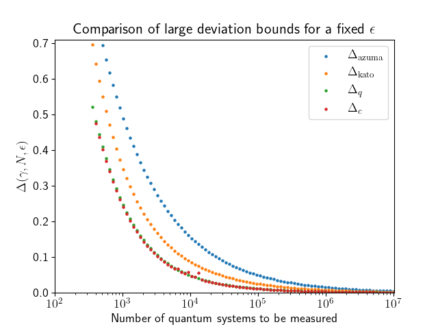
Figure 2: Comparison of the deviation $\Delta(\gamma,N,\epsilon)$ from (an upper bound on) the expectation value in Eqs. (141) and (145) when allowing the failure probability $\epsilon$. The parameters are chosen to be $\epsilon=10^{-30}$, $r=0.01$, and $B^{*}=0.01N$, and $\gamma$ is optimized to be $1.662$ so that an unconfirmed upper bound $\gamma B^{*}/N+m(\gamma)$ on $\hat{A}/N$ is minimized to be $0.02873$. We further assume that the random variable $\hat{B}$ is equal to the expected value $B^{*}$. The functions $\Delta_{\rm azuma}$ and $\Delta_{\rm kato}$ are defined respectively in Eqs. (152) and (160), and the functions $\Delta_{q}$, and $\Delta_{c}$ are defined implicitly through Eqs. (164) and (168).

We numerically demonstrate the tightness of these bounds in some cases. The first example is the case that is relevant to the finite-size analysis of the QKD. In QKD, the parameter $\epsilon$ is fixed and its value is typically chosen to be $\sim 10^{-30}$. In the QKD application, we have the expected value $B^{*}$ of $\hat{B}$ from the channel that we use for the transmission, which is the reason why Kato’s inequality [5] typically gives a tighter bound in the finite-size regime. For a model, we set $\epsilon=10^{-30}$, $r=0.01$, and $B^{*}=0.01N$. The parameter $\gamma$ in ${\cal A}(\gamma,\Delta)$ is chosen so that the expected (unconfirmed) upper bound $\gamma B^{*}/N+m(\gamma)$ on $\hat{A}/N$ in the limit $N\rightarrow\infty$ is minimized. In the choice of parameters above, we have $\gamma=1.662$ to give the expected asymptotic upper bound $0.02873$ on $\hat{A}/N$. We further assume the case in which $\hat{B}$ is exactly equal to $B^{*}$. Under these assumptions, we derive the deviation from the above asymptotic upper bound for finite $N$ allowing the failure probability $\epsilon$ with the four methods described above. Figure 2 shows the deviation $\Delta(\gamma,N,\epsilon)$ when varying the number $N$ of quantum systems to be measured. As the figure suggests, $\Delta_{c}$ defined through Eq. 168 is the smallest among four bounds in this setup and the above particular choices of parameters except for some points that may be caused by the insufficient optimization. We can also see that $\Delta_{q}$ defined through Eq. (164) gives the comparable bound. They are smaller than $\Delta_{\rm kato}$ defined in Eq. (160), while $\Delta_{\rm kato}$ is still smaller than the $\Delta_{\rm azuma}$ defined in Eq. (152).

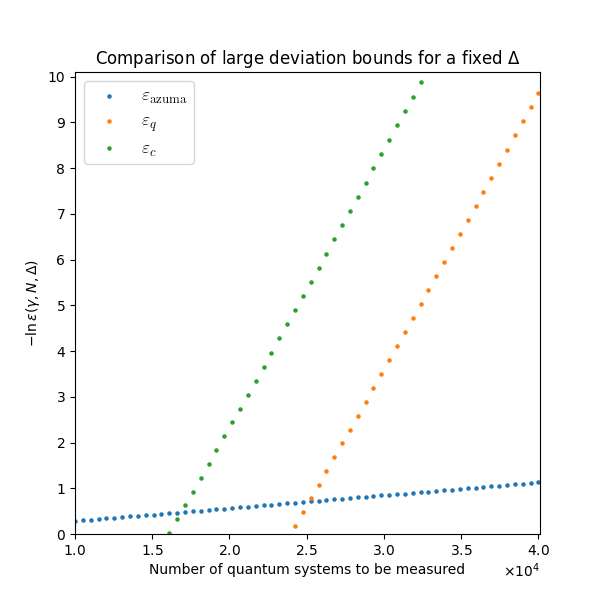
Figure 3: Comparison of the minus logarithm of the failure probability $\epsilon(\gamma,N,\Delta)$ in Eq. (146) against the number $N$ of measured quantum systems for a fixed value of the deviation $\Delta$. The parameters are chosen to be $\epsilon=10^{-30}$, $r=0.01$, and $B^{*}=0.01N$, and $\gamma$ is optimized to be $1.662$ so that an unconfirmed upper bound $\gamma B^{*}/N+m(\gamma)$ on $\hat{A}/N$ is minimized to be $0.02873$. We further assume that the random variable $\hat{B}$ is equal to the expected value $B^{*}$. The functions $\epsilon_{\rm azuma}$, $\epsilon_{q}$, and $\epsilon_{c}$ are defined in Eqs. (153), (165), and (169), respectively.

The next example is the case when we fix the deviation $\Delta$ from the expectation value (that is, an upper bound that holds in the asymptotic limit as shown in Eq. (149)) to a small value, and see how quickly the failure rate $\epsilon(\gamma,N,\Delta)$ in Eq. (146) goes to zero. We set the deviation $\Delta=0.01$, $r=0.01$ and $B^{*}=0.01N$, and choose $\gamma=1.662$ to give the asymptotically optimal upper bound $0.02873$ on $\hat{A}/N$ as was done in the previous figure. We also consider the case in which the observed value $\hat{B}$ is exactly equal to $B^{*}$. With these conditions, we plot $\epsilon_{\rm azuma}$ in Eq. (153), $\epsilon_{q}$ in Eq. (165), and $\epsilon_{c}$ in Eq. (169) in Fig. 3. As the figure suggests, the minus of each exponent, which governs the convergence speed, grows almost linearly for $N$, but its coefficient is very different between Azuma’s and ours. In fact, the convergence speed of our bounds is much faster than that of Azuma’s. Furthermore, $-\ln\epsilon_{q}$ and $-\ln\epsilon_{c}$ appear to have an almost constant gap. This gap exactly comes from the difference of the factors $f_{q}(N,d=2)\sim N^{\frac{3}{2}}$ and $f_{c}(N,k=3)\sim N$. We should note that there are regions in which Azuma’s inequality gives a better bound than ours when $N$ is small and the failure probability is large. When we alter the parameters $r$, $M$, and $\Delta$ in our model, then this region varies. However, our bound overall gives a faster convergence to the expectation value.

III.2 Application to quantum key distribution

For the next application, we consider Phoenix-Barnett-Chefles 2000 (PBC00) protocol [19], which uses three quantum states forming an equilateral triangle on the $X$-$Z$ plane in the Bloch sphere. The security of this protocol is proved in the finite-size case against general attacks in Ref. [2] using Azuma’s inequality. In order to make the paper as self-contained as possible, we list the protocol below. Let $\{\ket{0},\ket{1}\}$ be the $Z$ basis of a qubit. Let $\{\ket{+},\ket{-}\}$ with $\ket{\pm}\coloneqq(\ket{0}\pm\ket{1})/\sqrt{2}$ be the $X$ basis. The three states used in PBC00 protocol are $\ket{\psi_{1}}\coloneqq\cos(2\pi/3)\ket{+}+\sin(2\pi/3)\ket{-}$, $\ket{\psi_{2}}\coloneqq\cos(4\pi/3)\ket{+}+\sin(4\pi/3)\ket{-}$, and $\ket{\psi_{3}}\coloneqq\ket{+}$. Let us also define $\ket{\bar{\psi}_{i}}$ for $i=0,1,2$ that satisfies $\braket{\psi}{\bar{\psi}}=0$. Then, the PBC00 protocol is described as follows.

— PBC00 —

1. For each of $N$ rounds, Alice uniformly randomly generates a trit $\hat{r}_{i}$ and a bit $\hat{a}_{i}$, where $i\in\{1,\ldots,N\}$ denotes the label of the round. She chooses the pair $\{\ket{\psi_{1}},\ket{\psi_{2}}\}$ if $\hat{r}_{i}=0$, $\{\ket{\psi_{2}},\ket{\psi_{3}}\}$ if $\hat{r}_{i}=1$, and $\{\ket{\psi_{3}},\ket{\psi_{1}}\}$ if $\hat{r}_{i}=2$. If $\hat{a}_{i}=0(1)$, she sends the first (second) state of the chosen pair to Bob.

2. For each qubit received in the $i$-th round, Bob performs a measurement described by the POVM $\{\frac{2}{3}\ket{\bar{\psi}_{1}}\!\bra{\bar{\psi}_{1}},\frac{2}{3}\ket{\bar{\psi}_{2}}\!\bra{\bar{\psi}_{2}},\frac{2}{3}\ket{\bar{\psi}_{3}}\!\bra{\bar{\psi}_{3}}\}$.

3. After the $N$ rounds of communication, Alice announces the sequence of trits $\{\hat{r}_{i}\}_{i=1}^{N}$. Bob defines $\hat{b}_{i}=0(1)$ if $\hat{r}_{i}=0$ and his measurement outcome in the $i$-th round is $\ket{\bar{\psi}_{2}}$ ($\ket{\bar{\psi}_{1}}$), if $\hat{r}_{i}=1$ and his measurement outcome in the $i$-th round is $\ket{\bar{\psi}_{3}}$ ($\ket{\bar{\psi}_{2}}$), and if $\hat{r}_{i}=2$ and his measurement outcome in the $i$-th round is $\ket{\bar{\psi}_{1}}$ ($\ket{\bar{\psi}_{3}}$). All other events are regarded as inconclusive. Bob announces whether his measurement is inconclusive or not for each $i$. Alice and Bob keep $\hat{a}_{i}$ and $\hat{b}_{i}$, respectively, when Bob’s outcome in the $i$-th round is conclusive. Let $\hat{N}_{\rm con}$ be the number of conclusive rounds.

4. For each element of the $\hat{N}_{\rm con}$-bit sequence that Alice keeps in the previous step, Alice uniformly randomly chooses the label “test” or “sift” and announces it. Let $\hat{N}_{\rm test}$ and $\hat{N}_{\rm sift}$ be the number of test and sift bits, respectively, which satisfies $\hat{N}_{\rm con}=\hat{N}_{\rm test}+\hat{N}_{\rm sift}$. Alice and Bob announce all the bits labeled by “test” and estimate the bit error rate. From the estimated bit error rate, they perform a bit error correction on the sifted key, i.e., $\hat{N}_{\rm sift}$-bit sequence labeled by “sift”. Let $\hat{N}_{\rm KC}$ be the number of pre-shared secret keys consumed during the bit error correction.

5. Alice and Bob agree on the amount $\hat{N}_{\rm PA}$ of privacy amplification and perform the linear hash function to obtain the final key.

As can be seen from the protocol, the net key gain $\hat{G}$ per communication rounds of this protocol can be given by

$$\hat{G}=(\hat{N}_{\rm sift}-\hat{N}_{\rm KC}-\hat{N}_{\rm PA})/N.$$ (170)

In Ref. [8], the protocol is shown to be secure in the finite-size regime by the so-called phase error correction approach [20, 21, 22]. In fact, if we consider the purified version of the protocol defined above in which Alice instead prepares an entangled state $\ket{\Psi}_{AB}\coloneqq(\ket{0}_{A}\otimes R_{y}(2\pi\hat{r}_{i}/3)\ket{\psi_{1}}_{B}+\ket{1}_{A}\otimes R_{y}(2\pi(\hat{r}_{i}+1)/3)\ket{\psi_{1}}_{B})\sqrt{2}$, where $R_{y}(\theta)$ denotes the $\theta$ rotation around $y$ axis in the Bloch sphere, and sends the system $B$ to Bob, then the security of the key can be reduced to how much maximally entangled state $\ket{\Phi}_{AB}\coloneqq(\ket{0}_{A}\ket{0}_{B}+\ket{1}_{A}\ket{1}_{B})/\sqrt{2}$ Alice and Bob can extract in this purified protocol. Thus, the bit error operator $\Pi_{\rm bit}$ and phase error operator $\Pi_{\rm ph}$ can be defined, which correspond to the event that they obtain bit and phase flipped maximally entangled states, respectively, in the purified protocol. Explicitly, $\Pi_{\rm bit}$ and $\Pi_{\rm ph}$ are given by [8]

$$\begin{split}\Pi_{\rm bit}&=\frac{1}{3}\sum_{r=0}^{2}\Bigl{[}\ket{0}\!\bra{0}_{A}\otimes R_{y}\Bigl{(}\frac{2\pi r}{3}\Bigr{)}F\ket{1}\!\bra{1}_{B}FR_{y}\Bigl{(}-\frac{2\pi r}{3}\Bigr{)}\\ &\qquad\quad+\ket{1}\!\bra{1}_{A}\otimes R_{y}\Bigl{(}\frac{2\pi r}{3}\Bigr{)}F\ket{0}\!\bra{0}_{B}FR_{y}\Bigl{(}-\frac{2\pi r}{3}\Bigr{)}\Bigr{]},\end{split}$$ (171)

$$\begin{split}\Pi_{\rm ph}&=\frac{1}{3}\sum_{r=0}^{2}\Bigl{[}\ket{+}\!\bra{+}_{A}\otimes R_{y}\Bigl{(}\frac{2\pi r}{3}\Bigr{)}F\ket{-}\!\bra{-}_{B}FR_{y}\Bigl{(}-\frac{2\pi r}{3}\Bigr{)}\\ &\qquad\quad+\ket{-}\!\bra{-}_{A}\otimes R_{y}\Bigl{(}\frac{2\pi r}{3}\Bigr{)}F\ket{+}\!\bra{+}_{B}FR_{y}\Bigl{(}-\frac{2\pi r}{3}\Bigr{)}\Bigr{]},\end{split}$$ (172)

where the filter operator $F\coloneqq\ket{0}\!\bra{0}+\frac{1}{\sqrt{3}}\ket{1}\!\bra{1}$. From these, we can derive the following [8]:

$$\Pi_{\rm ph}\leq\frac{5}{4}\Pi_{\rm bit}.$$ (173)

Since the bit error rate $e_{\rm bit}$ can directly be observed in the “test” rounds, the asymptotic key rate $\hat{G}_{\rm aympt}$ of this protocol can be given by

$$\hat{G}_{\rm asympt}=\frac{1}{4}\left(1-h(e_{\rm bit})-h\Bigl{(}\frac{5}{4}e_{\rm bit}\Bigr{)}\right),$$ (174)

where $h(x)\coloneqq-x\log_{2}x-(1-x)\log_{2}(1-x)$ denotes the binary-entropy function. In the above, the prefactor $1/4$ comes from the fact that the measurement is conclusive with the probability $1/2$ (without Eve’s attack) and that the “sift” is chosen with the probability $1/2$. In the finite-size case, however, we need to take into account the statistical fluctuations. Let us consider the purified protocol again and $\hat{x}_{\rm bit}^{(i)}$ be a random variable at $i$-th round that takes the value one when “test” is chosen and the bit error is observed while takes zero otherwise. Then, $\hat{N}_{\rm bit}\coloneqq\sum_{i=1}^{N}\hat{x}_{\rm bit}^{(i)}$ corresponds to the number of bit error observed in the protocol. Let $\hat{x}_{\rm ph}^{(i)}$ be another random variable at $i$-th round that takes the value one when “sift” is chosen and the phase error occurs while takes zero otherwise. Then, $\hat{N}_{\rm ph}\coloneqq\sum_{i=1}^{N}\hat{x}_{\rm ph}^{(i)}$ corresponds to the number of phase errors in the sifted key. It is known that if we can show

$$\mathrm{Pr}[\hat{N}_{\rm ph}\geq U(\hat{N}_{\rm bit})]\leq\epsilon,$$ (175)

for a function $U(\hat{N}_{\rm bit})$ of $\hat{N}_{\rm bit}$, and by setting

$$\hat{N}_{\rm PA}=\hat{N}_{\rm sift}h(U(\hat{N}_{\rm bit})/\hat{N}_{\rm sift})+s,$$ (176)

then the protocol is $\sqrt{2(\epsilon+2^{-s})}$-secret [22, 23, 24]. Furthermore, we assume that the secret-key consumption in the bit error correction at Step 4 of the protocol is given by

$$\hat{N}_{\rm KC}=\hat{N}_{\rm sift}h(\hat{N}_{\rm bit}/\hat{N}_{\rm sift})+s^{\prime},$$ (177)

for sending an $\hat{N}_{\rm sift}h(\hat{N}_{\rm bit}/\hat{N}_{\rm sift})$-bit syndrome string and $s^{\prime}$-bit verification string to ensure $2^{-s^{\prime}}$-correctness. Thus, if we can obtain the function $U(\cdot)$ to satisfy Eq. (175), we can obtain a key rate in the finite-size case as well satisfying $2^{-s^{\prime}}$-correctness and $\sqrt{2(\epsilon+2^{-s})}$-secrecy.

The derivation of Eq. (175) is very similar to the one in the previous section. When Azuma’s or Kato’s is applied to the problem, the operator inequality (173) can be used as an inequality between the conditional expectations of $\hat{x}_{\rm bit}^{(i)}$ and $\hat{x}_{\rm ph}^{(i)}$. By applying Azuma’s inequality to $\hat{x}_{\rm ph}^{(i)}-\frac{5}{4}\hat{x}_{\rm bit}^{(i)}$, we have

$$\mathrm{Pr}\left[\frac{\hat{N}_{\rm ph}}{N}-\frac{5}{4}\frac{\hat{N}_{\rm bit}}{N}\geq\left(1+\frac{5}{4}\right)\sqrt{\frac{\ln(1/\epsilon)}{2N}}\right]\leq\epsilon.$$ (178)

In this case, the function $U_{\rm azuma}$ to satisfy Eq. (175) should be

$$U_{\rm azuma}(\hat{N}_{\rm bit})=\frac{5}{4}\hat{N}_{\rm bit}+\frac{9}{4}\sqrt{\frac{N\ln(1/\epsilon)}{2}}.$$ (179)

Similarly, by applying Kato’s inequality to $\hat{x}_{\rm bit}^{(i)}$ while applying Azuma’s inequality to $\hat{x}_{\rm ph}^{(i)}$, we have

$$\begin{split}\mathrm{Pr}\Biggl{[}\frac{\hat{N}_{\rm ph}}{N}-\frac{5}{4}\frac{\hat{N}_{\rm bit}}{N}&\geq\sqrt{\frac{\ln(2/\epsilon)}{2N}}\\ &\quad+\frac{5}{4\sqrt{N}}\biggl{[}\beta-\alpha\Bigl{(}1-\frac{2\hat{N}_{\rm bit}}{N}\Bigr{)}\biggr{]}\Biggr{]}\leq\epsilon,\end{split}$$ (180)

$$\alpha \coloneqq\alpha^{*}(N_{\rm bit}^{*},N,\epsilon/2),$$ (181)

$$\beta \coloneqq\beta^{*}(N_{\rm bit}^{*},N,\epsilon/2),$$ (182)

where the functions $\alpha^{*}$ and $\beta^{*}$ are defined in Eqs. (155) and (156) with $N_{\rm bit}^{*}$ being an unconfirmed knowledge of $\hat{N}_{\rm bit}$ prior to the protocol. The function $U_{\rm kato}$ to satisfy Eq. (175) should thus be

$$\begin{split}U_{\rm kato}(\hat{N}_{\rm bit})&=\frac{5}{4}\hat{N}_{\rm bit}+\sqrt{\frac{N\ln(2/\epsilon)}{2}}\\ &\qquad+\frac{5\sqrt{N}}{4}\left(\beta-\alpha\left(1-\frac{2\hat{N}_{\rm bit}}{N}\right)\right).\end{split}$$ (183)

Now we apply Theorem 1 to this protocol. Let ${\cal X}\coloneqq\{\text{phase error in ``sift''},\text{bit error in ``test''},\text{others}\}$ be a sample space, and $\bm{p}=(p_{1},p_{2},p_{3})$ be a probability mass function on ${\cal X}$. Then, from Eq. (173), the set ${\cal Q}$ of allowed probability mass function for any quantum state between Alice and Bob can be given by

$${\cal Q}=\left\{\bm{p}=(p_{1},p_{2},p_{3}):p_{1}\leq\frac{5}{4}p_{2}\right\},$$ (184)

where we used the fact that “sift” and “test” rounds are chosen with equal probability. Thus, for any i.i.d. quantum state $\rho_{AB}^{\otimes N}$ between Alice and Bob, we have

$$\begin{split}&\mathrm{Pr}\left[\left(\frac{\hat{N}_{\rm ph}}{N},\frac{\hat{N}_{\rm bit}}{N},1-\frac{\hat{N}_{\rm ph}}{N}-\frac{\hat{N}_{\rm bit}}{N}\right)\in{\cal A}(\delta)\middle|\rho_{AB}^{\otimes N}\right]\\ &\leq\max_{\bm{p}\in{\cal A}(\delta)}\max_{\bm{q}\in{\cal Q}}\exp[-ND(\bm{p}\|\bm{q})],\end{split}$$ (185)

from Sanov’s theorem [6, 7], where ${\cal A}(\delta)$ is defined as

$${\cal A}(\delta)=\left\{\bm{p}=(p_{1},p_{2},p_{3}):p_{1}\geq\frac{5}{4}p_{2}+\delta\right\}.$$ (186)

Now, since the number of bit and phase errors is invariant under the permutation of rounds, we can virtually permute the four-dimensional quantum system between Alice and Bob in the purified protocol across the rounds. Thus, we can apply Theorem 1 to the above and obtain

$$\begin{split}&\mathrm{Pr}\left[\left(\frac{\hat{N}_{\rm ph}}{N},\frac{\hat{N}_{\rm bit}}{N},1-\frac{\hat{N}_{\rm ph}}{N}-\frac{\hat{N}_{\rm bit}}{N}\right)\in{\cal A}(\delta)\right]\\ &\leq\max_{\bm{p}\in{\cal A}(\delta)}\max_{\bm{q}\in{\cal Q}}f_{q}(N,4)\exp[-ND(\bm{p}\|\bm{q})].\end{split}$$ (187)

We should optimize the value $\delta$ in the above so that the right-hand side is smaller than or equal to $\epsilon$. If we write such an optimized $\delta$ in this case as $\delta_{q}$, the function $U_{q}$ to satisfy Eq. (175) is given by

$$U_{q}(\hat{N}_{\rm bit})=\frac{5}{4}\hat{N}_{\rm bit}+\delta_{q}.$$ (188)

Finally, we apply Theorem 3 to this problem. We can regard the measurement in the purified protocol as the three-outcome measurement channel as described above. Since the set of probability mass functions after measurement is included in ${\cal Q}$ in Eq. (184), which is already linear and contains all the extremal points of the convex polytope of the probability mass functions except $(1,0,0)$, we can choose ${\cal R}={\cal Q}$, where ${\cal R}$ is defined in Theorem 3. The region ${\cal R}^{\prime}$ in Theorem 3 is thus given by

$$\begin{split}{\cal R}^{\prime}&=\Biggl{\{}\bm{p}=(p_{1},p_{2},p_{3}):\\ &\hskip 28.45274ptp_{1}-\frac{5}{4}p_{2}\leq\frac{\sqrt{2}}{N}\sqrt{\left(\frac{13}{12}\right)^{2}+\left(-\frac{14}{12}\right)^{2}+\left(\frac{1}{12}\right)^{2}}\Biggr{\}}.\end{split}$$ (189)

Therefore, from Theorem 3, we have

$$\begin{split}&\mathrm{Pr}\left[\left(\frac{\hat{N}_{\rm ph}}{N},\frac{\hat{N}_{\rm bit}}{N},1-\frac{\hat{N}_{\rm ph}}{N}-\frac{\hat{N}_{\rm bit}}{N}\right)\in{\cal A}(\delta)\right]\\ &\leq\max_{\bm{p}\in{\cal A}(\delta)}\max_{\bm{q}\in{\cal R}^{\prime}}f_{c}(N,3)\exp[-ND(\bm{p}\|\bm{q})].\end{split}$$ (190)

In the same way as the previous discussion, the value $\delta$ should be optimized so that the right-hand side above is smaller than or equal to $\epsilon$. Let $\delta_{c}$ be such a value. Then, the function $U_{c}$ to satisfy Eq. (175) in this case is given by

$$U_{c}(\hat{N}_{\rm bit})=\frac{5}{4}\hat{N}_{\rm bit}+\delta_{c}.$$ (191)

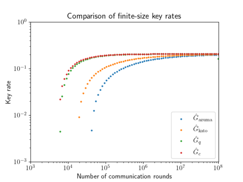
Figure 4: Comparison of key rates against the total number $N$ of rounds when the bit error rate is one percent. The key rates are given by the formula (192), where the function $U$ is either $U_{\rm azuma}$ in Eq. (179), $U_{\rm kato}$ in Eq. (183), $U_{q}$ in Eq. (188), or $U_{c}$ in Eq. (191) with the parameter $\epsilon=2^{-102}$. The parameters $s$ and $s^{\prime}$ in Eq. (192) are chosen to be $s=102$ and $s^{\prime}=50$ so that the correctness and secrecy parameter of the protocol are both $2^{-50}$.

We compare the key rates obtained through the different concentration inequalities that give the functions Eqs. (179), (183), (188), and (191), respectively. We set $\epsilon=2^{-102}$, $s=102$, and $s^{\prime}=50$ so that the secrecy and correctness parameters are $2^{-50}$, which are conventional values. We also assume that the number $\hat{N}_{\rm con}$ of conclusive events is equal to its expectation value $N/2$ and that the length $\hat{N}_{\rm sift}$ of the sifted key is equal to its expectation value $N/4$. The observed bit error rate is one percent, i.e., $\hat{N}_{\rm bit}=(N_{\rm con}-\hat{N}_{\rm sift})/100=N/400$. Under these assumptions, we computed the key rate $\hat{G}$ with respect to the total number $N$ of rounds, where $\hat{G}$ is given from Eqs. (170), (176), and (177) by:

$$\hat{G}=\frac{\hat{N}_{\rm sift}[1-h(\hat{N}_{\rm bit}/\hat{N}_{\rm sift})-h(U(\hat{N}_{\rm bit})/\hat{N}_{\rm sift})]-s-s^{\prime}}{N}.$$ (192)

In the above, the function $U$ is either $U_{\rm azuma}$, $U_{\rm kato}$, $U_{q}$, or $U_{c}$. Figure 4 shows the comparison of the key rates against $N$ with the above four different concentration inequalities applied. The figure shows that our concentration inequalities derived through Theorem 1 and 3 are better than those obtained through Azuma’s and Kato’s inequalities. Therefore, also in this illustrated example, the Sanov-type quick convergence predominates over the polynomial factors in Eqs. (188) and (191).

IV Discussion

In this paper, we developed concentration inequalities for a permutation-invariant quantum state possibly with an additional symmetry and a sequence of outcomes of independent and identical quantum measurements performed on an adversarial quantum state. For the former case, we used the technique from the representation theory of the permutation group, which is well-known in the community of quantum information theory. With this rather conventional technique, we can upper-bound the permutation-invariant state by i.i.d. quantum states. Compared to the previous de-Finetti-type statement [9, 10, 11], our improvement for this case comes from the fact that one can adaptively choose these i.i.d. states depending on the irreducible subspace of the permutation group. For the latter case, we found an upper bound on the probability of obtaining each sequence of quantum measurement outcomes with a specific type and then obtained a concentration inequality for the probability of obtaining sequences with the atypical types. For this, we developed, to the best of the author’s knowledge, a completely new technique that uses a geometric structure of the convex polytope of the probability mass functions in which the set of types is contained as lattice points. Both bounds we obtained are Sanov-type and are thus tighter than the conventional bound obtained via Azuma’s inequality. In specific models we discussed in Sec. III, our bounds even outperform the recently developed refinement of Azuma’s inequality [5]. Even though the applicability of our bounds is limited compared to Azuma-type inequalities, they still have many applications in QKD as demonstrated in Sec. III.2 and possibly in other quantum information theories to mitigate finite-size effects.