Memory formation in dense persistent active matter
Abstract
Protocol-dependent states in structural glasses can encode a disordered, yet retrievable memory. While training such materials is typically done via a global drive, such as external shear, in dense active matter the driving is instead local and spatio-temporally correlated. Here we focus on the impact of such spatial correlation on memory formation. We investigate the mechanical response of a dense amorphous packing of athermal particles, subject to an oscillatory quasistatic driving with a tunable spatial correlation, akin to the instantaneous driving pattern in active matter. We find that the capacity to encode memory can be rendered comparable upon a proper rescaling on the spatial correlation, whereas the efficiency in memory formation increases with motion cooperativity.
Introduction.
Driven amorphous solids have recently shown great promise in understanding and characterizing material memory [1, 2]. While structural disorder renders theoretical descriptions challenging [3], it can also be harnessed to engineer specific disorder-induced properties [4, 5, 6]. From a memory perspective, specific states can be encoded—and retrieved—with carefully tailored driving protocols. The challenge is then to characterize which states can be reached [7, 8, 9, 10], and with how much training. One class of such mechanical trainings are oscillatory athermal quasistatic shear, either in particle-based [11, 12, 13, 14, 15] or coarse-grained models [16, 17, 18, 19]. Here, a system is cyclically sheared starting from a given initial condition, typically at equilibrium, and may eventually reach a hysteretic limit cycle. Depending on the maximum strain, its mechanical response displays a dynamical yielding transition from a regime where return-point memory is achievable to a regime where plastic rearrangements prevent memory formation [20].
In parallel, a considerable effort is being deployed to understand dense active matter. A central goal is to assess which phenomena from amorphous solids with passive individual components are relevant, and thus exportable, to interacting active particles [21, 22, 23]. Characterizing the interplay between structural disorder and activity has become a flourishing field, e.g. to investigate the role mechanical signalling in confluent tissues [24, 25, 26, 27, 28, 29, 30, 31, 32, 33, 34, 35, 23]. The key novelty is that active systems are driven locally, at the scale of their individual components, instead of globally [36]. Nevertheless, active systems experience plasticity in sufficiently dense regimes, affecting both their mechanical and rheological properties. In light of this, we have established a direct link between global shear and spatially-correlated local driving [37], akin to the instantaneous self-propulsion in active matter [33].
In this Letter, we focus on the role of such spatial correlation on memory formation. Building on the connection predicted and tested in [37, 38], we investigate the mechanical response of a dense amorphous packing of athermal particles, subject to an oscillatory driving pattern with a tunable spatial correlation. We focus on their stress-strain curves, which display a hysteretic behavior depending on the maximum strain and number of cycles. Memory is quantified by comparing successive snapshots of configurations after each cycle.
Our study shows that by tuning the spatial correlation of the local driving, we can control both the capacity and efficiency to reach a limit cycle, and therefore to encode a memory. Our findings suggest that increasing motion cooperativity is a generic strategy to enhance memory formation.
Model and driving protocol.
Simulations are performed on dense packings of bidisperse Hertzian disks with a size ratio and number ratio, under periodic boundary conditions in a square box of size . The position of particle is given by . We initialize the system at with the standard prescription of [39]: particles are uniformly distributed via a Poisson process (corresponding to an infinite temperature quench) at a packing fraction —well above the jamming transition [40]—and minimized via the FIRE protocol [41] until the inherent state is found, while keeping the density fixed. Distance units are chosen such that the smaller particles have unit diameter, thus and an average interparticle distance . The results of [37, 42, 43, 44, 45] suggest that our choice of will quantitatively change certain scales, but not fundamentally alter the physics, provided that .
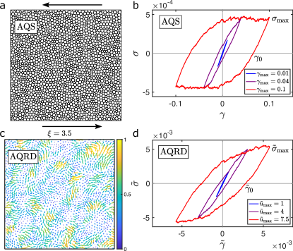
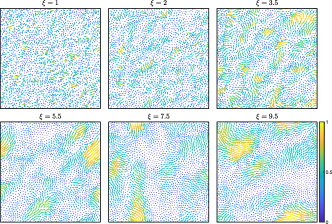
We consider two protocols illustrated in Fig. 1: a global athermal quasistatic shear (AQS) [46] and a local athermal quasistatic random displacement (AQRD) [37]. Full details of each implementation are given in the above references. For AQS, we use Lees-Edwards boundary conditions to apply a dimensionless strain increment , minimize via FIRE, and measure the corresponding stress using the Born-Huang approximation [47]. The total accumulated strain is denoted , and the corresponding shear stress . For AQRD, we assign to each particle a local displacement vector that we keep constant. We label the tunable driving pattern , with the ket notation indicating an -dimensional vector. Throughout this work, we generate a Gaussian field of correlation length as in [37], and combine it with the initial configuration . This is akin to freezing the instantaneous velocity field in dense active matter, or alternatively working at timescales smaller than the persistence time. A displacement increment is then applied along , and a constrained minimization (via FIRE) is performed using a Lagrange multiplier along , globally prohibiting motion along . The total accumulated AQRD displacement is denoted . For AQRD, the relevant random ‘strain’ and ‘stress’ are defined, respectively, as
| (1) |
where is the dimensional residual force. Between plastic rearrangements, an apparent elastic modulus can be defined as .
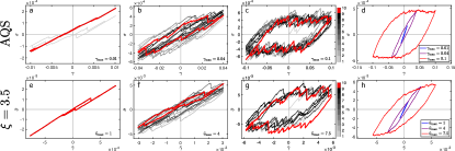
In both AQS and AQRD, we apply an oscillatory strain such that strain/displacement is incrementally increased to , then similarly decreased to , and the process is repeated. Each full cycle is labelled by the integer . We consider the same 30 initial seed configurations, which fix both and the initial driving field . We record the corresponding stress-strain curves and , along with successive snapshots of the system at maximum strains. The simulations thus depend on the maximum driving amplitude , the total number of cycles , and the spatial correlation for AQRD. Typical mechanical responses are illustrated in Fig. 1 at our last cycle . See SI for more details on the numerics, the range of explored parameters, and examples of individual trajectories.
Driving pattern characterization vs average elastic modulus.
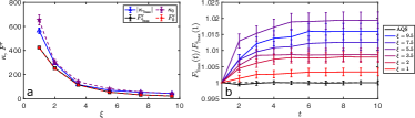
The analytical predictions in [37, 38] suggest a statistical equivalence between AQS-AQRD stress-strain curves, provided that we compare the AQS strain to the effective random strain , and the AQS shear stress to . The rescaling factor is measured as the ratio of the average apparent modulus (of the driving pattern ), to its counterpart (under global shear). This ratio depends on the disorder of the driving pattern, decreasing with increased cooperativity (i.e. larger ). For pairwise-interacting particles, this is quantified by the variance of relative displacements on interacting pairs nondimensionalized with , denoted . The analytical prediction further states that , providing a direct and straightforward link between the mechanical response of the dense packing and the statistical features of the driving pattern [37, 38].
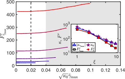
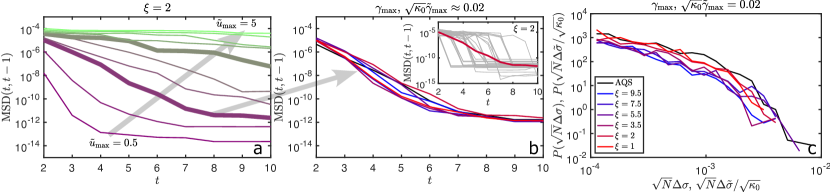
Both and are physical quantities measurable in an agnostic way from a given snapshot of the system (see SI). We denote their initial values , and at the maximum strain in the last cycle , presumably in the limit cycle, if it exists. We report their values in Fig. 2 for different driving correlation . To make these values comparable, we rescale the random strain with the initial , so as not to depend on the subsequent driving protocol. We see that is constant for , which is roughly the yielding point as discussed later (see Fig. 3). The variance significantly increases beyond that, as can be seen for the three smallest- curves, showing that the driving pattern has become more disordered (i.e. effectively a smaller ) upon cycling; and above , we later show that a limit cycle is not reached per se. In the inset, we show the -dependence at a small effective strain , by selecting maximum effective strains carefully for each . As expected, follows the same decreasing trend as the pattern variance ; physically, it is easier to deform a material with larger motion cooperativity because it has a lower apparent elastic modulus.
A fixed driving pattern is implicitly enforced in our analytical predictions [37, 38], as particle displacements are then restricted to a distance in the limit of dimension . Note that we restricted ourselves to AQRD protocols with , so that this initial pattern mostly survives upon successive cycles, despite the plastic rearrangements occurring until (and at) the limit cycles. This guarantees that our driving protocol keeps the system within the validity range of the infinite-dimensional limit predictions. The overall persistence of the initial pattern is confirmed by and , further supporting our choice of to rescale all subsequent plots.
Collapsing the averaged limit cycles.
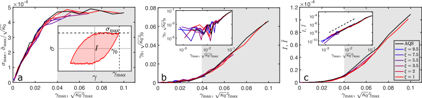
We can now use this rescaling to compare the stress-strain curves as plotted in Fig. 1. The relevance of the infinite-dimensional analytical predictions for our model was successfully tested in [37] but only in the pre-yielding regime starting from , i.e. in the very first cycle of our oscillatory protocol. Here we use it as a tool to render comparable the geometrical features of mechanical hysteresis, as defined and plotted in Fig. 3: for AQS, for AQRD, where and . These quantities are measured and averaged on the last cycle as in Fig. 1, presumably at the limit cycle (when reachable). As predicted analytically [38], we find that they can be collapsed onto master curves using the initial ratio . Thus the mechanical response for a given local displacement under oscillatory AQRD can be pushed either inside or outside an effective ‘pre-yielding’ regime, simply by tuning the spatial correlation of the driving pattern. This explains why the simulation range is effectively compressed in Fig. 3 when increasing . On the other hand, increasing cooperativity promotes an increased efficiency for a given strain, i.e. less dissipated energy per cycle .
Memory characterization.
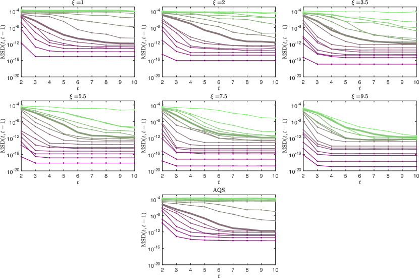
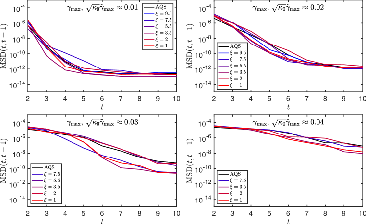
We now examine the implications of these findings for memory formation. We quantify the convergence to a limit cycle by comparing successive stroboscopic snapshots at the maximum strain at each cycle , with the mean-square-displacement (MSD) of the difference, where brackets denote the average over initial configurations. By increasing the maximum strain we cross over from a regime with an exponential decay to a limit cycle to a regime where the existence of a limit cycle is not warranted [Fig. 4(a)]. This crossover occurs at the ‘yielding point’ already evidenced in Fig. 3(a). At sufficiently large , plastic rearrangements prevent the system from locking into a limit cycle, yielding a finite MSD plateau when comparing configurations stroboscopically. This threshold can be tuned with the motion cooperativity [Fig. 3]: Fig. 4(b) shows how the same rescaling can further be used to collapse the averaged memory decay upon AQRD cycling. Put simply, a limit cycle (memory) can be achieved in a similar way (e.g. same number of cycles) by jointly tuning and so as to keep the effective strain fixed. In practice, when increasing the motion cooperativity, a smaller absolute strain is typically required to achieve the same memory training.
Mean-field statistical features in the limit cycles.
In [37], the link between AQS and AQRD was shown on three mean-field metrics of the disordered landscape explored by a typical glassy system—via the collapse of the elastic-modulus, the stress-drops and strain-steps distributions—in the very first cycle. Fig. 4(c) shows similarly a good collapse of the stress-drop distributions at the last cycle, for the same composite dataset at small effective strain. This then supports the claim that the predicted scaling holds for the statistical features of the landscape visited along the whole AQRD/AQS training.
Conclusion.
We examined the role of motion cooperativity in memory formation, focusing on oscillatory driving protocols under spatially-correlated local driving. We found that the hysteretic mechanical response could be rendered comparable by rescaling the stress-strain curves with , as predicted in [37, 38], and that this connection applies to memory dynamics as well. Increasing the driving spatial correlation pushes the system towards the pre-yielding regime where memory is achievable, (i) with a more efficient training (i.e. less energy dissipated per cycle) and (ii) requiring lower maximum strain to reach a given target state.
Conversely, more localized fields open the possibility to encode multiple localized memories into the same sample, of great interest for materials engineering.
In genuine dense active matter, the velocity field can be self-generated [33] or externally tuned, for instance, by chemical signalling in biological tissues [48] or remote-sync in crowds. Our findings suggest that allowing for more cooperativity is a good strategy to robustly and efficiently encode memory in a structurally disordered system. Here we focused on the role of spatial correlation, but its interplay with a finite persistence time remains an open issue [49, 50], as reinstating time also implies moving beyond the quasistatic limit. For extremely persistent active systems and small driving amplitude, the protocol of [51, 52] could be adapted to include a finite spatial correlation in a quasistatic-like settings. Hence we speculate that our findings extend at low driving rate—given precautions to stay within the validity range of these predictions—albeit with additional challenges to rationalize memory formation at finite rates [53].
At a more abstract level, our oscillatory AQRD protocol allows us to tune the energy landscape effectively explored by the system. The exact AQS/AQRD equivalence in infinite dimension [38] extends to the mean-field statistical features of this landscape. A corollary issue is thus to understand how its complex structure is spatially connected—casting it for instance on random transition graphs between mechanically stable configurations as for AQS [54, 55, 56, 57]—using our imposed cooperativity as an artificial probe of the underlying graph topology. This would be key to understanding which types of memory can be encoded in dense active matter.
Acknowledgements.
E.A. acknowledges partial support from the Swiss National Science Foundation by the SNSF Ambizione Grant No. PZ00P2_173962, and from the Simons Foundation (Grant No. 348126 to S. Nagel). The simulations were developed at Princeton University on the Adroit cluster and performed at the University of Geneva on the Mafalda cluster.References
- [1] Nathan C. Keim, Joseph D. Paulsen, Zorana Zeravcic, Srikanth Sastry, and Sidney R. Nagel. Memory formation in matter. Rev. Mod. Phys. 91, 035002 (2019).
- [2] Sidney R. Nagel, Srikanth Sastry, Zorana Zeravcic, and Murugappan Muthukumar. Memory formation. The Journal of Chemical Physics 158, 210401 (2023).
- [3] Glasses and aging: A Statistical Mechanics Perspective. Encyclopedia of Complexity and Systems Science (2022) 2020.
- [4] Muamer Kadic, Graeme W. Milton, Martin van Hecke, and Martin Wegener. 3D metamaterials. Nature Reviews Physics 1, 198 (2019).
- [5] Sunkyu Yu, Cheng-Wei Qiu, Yidong Chong, Salvatore Torquato, and Namkyoo Park. Engineered disorder in photonics. Nature Reviews Materials 6, 226 (2021).
- [6] Nitin Upadhyaya and Ariel Amir. Disorder engineering: From structural coloration to acoustic filters. Phys. Rev. Mater. 2, 075201 (2018).
- [7] Srikanth Sastry, Pablo G. Debenedetti, and Frank H. Stillinger. Signatures of distinct dynamical regimes in the energy landscape of a glass-forming liquid. Nature 393, 554 (1998).
- [8] Misaki Ozawa, Takeshi Kuroiwa, Atsushi Ikeda, and Kunimasa Miyazaki. Jamming Transition and Inherent Structures of Hard Spheres and Disks. Phys. Rev. Lett. 109, 205701 (2012).
- [9] Patrick Charbonneau and Peter K. Morse. Memory Formation in Jammed Hard Spheres. Phys. Rev. Lett. 126, 088001 (2021).
- [10] Patrick Charbonneau and Peter K. Morse. Jamming, relaxation, and memory in a minimally structured glass former. Phys. Rev. E 108, 054102 (2023).
- [11] Takeshi Kawasaki and Ludovic Berthier. Macroscopic yielding in jammed solids is accompanied by a nonequilibrium first-order transition in particle trajectories. Phys. Rev. E 94, 022615 (2016).
- [12] Premkumar Leishangthem, Anshul D. S. Parmar, and Srikanth Sastry. The yielding transition in amorphous solids under oscillatory shear deformation. Nature Communications 8, 14653 (2017).
- [13] Monoj Adhikari and Srikanth Sastry. Memory formation in cyclically deformed amorphous solids and sphere assemblies. The European Physical Journal E 41, 105 (2018).
- [14] Wei-Ting Yeh, Misaki Ozawa, Kunimasa Miyazaki, Takeshi Kawasaki, and Ludovic Berthier. Glass Stability Changes the Nature of Yielding under Oscillatory Shear. Phys. Rev. Lett. 124, 225502 (2020).
- [15] Himangsu Bhaumik, Giuseppe Foffi, and Srikanth Sastry. The role of annealing in determining the yielding behavior of glasses under cyclic shear deformation. PNAS 118, e2100227118 (2021).
- [16] Kareem Khirallah, Botond Tyukodi, Damien Vandembroucq, and Craig E. Maloney. Yielding in an Integer Automaton Model for Amorphous Solids under Cyclic Shear. Phys. Rev. Lett. 126, 218005 (2021).
- [17] D. Kumar, S. Patinet, C. E. Maloney, I. Regev, D. Vandembroucq, and M. Mungan. Mapping out the glassy landscape of a mesoscopic elastoplastic model. The Journal of Chemical Physics 157, 174504 (2022).
- [18] Chen Liu, Ezequiel E. Ferrero, Eduardo A. Jagla, Kirsten Martens, Alberto Rosso, and Laurent Talon. The fate of shear-oscillated amorphous solids. The Journal of Chemical Physics 156, 104902 (2022).
- [19] Jack T. Parley, Srikanth Sastry, and Peter Sollich. Mean-Field Theory of Yielding under Oscillatory Shear. Phys. Rev. Lett. 128, 198001 (2022).
- [20] Ido Regev, John Weber, Charles Reichhardt, Karin A. Dahmen, and Turab Lookman. Reversibility and criticality in amorphous solids. Nature Communications 6, 8805 (2015).
- [21] Liesbeth M C Janssen. Active glasses. J. Phys.: Condens. Matter 31, 503002 (2019).
- [22] Ludovic Berthier, Elijah Flenner, and Grzegorz Szamel. Glassy dynamics in dense systems of active particles. The Journal of Chemical Physics 150, 200901 (2019).
- [23] Thibaut Divoux, Elisabeth Agoritsas, Stefano Aime, Catherine Barentin, Jean-Louis Barrat, Roberto Benzi, Ludovic Berthier, Dapeng Bi, Giulio Biroli, Daniel Bonn, Philippe Bourrianne, Mehdi Bouzid, Emanuela Del Gado, Hélène Delanoë-Ayari, Kasra Farain, Suzanne Fielding, Matthias Fuchs, Jasper van der Gucht, Silke Henkes, Maziyar Jalaal, Yogesh M. Joshi, Anaël Lemaître, Robert L. Leheny, Sébastien Manneville, Kirsten Martens, Wilson C.K. Poon, Marko Popović, Itamar Procaccia, Laurence Ramos, James A. Richards, Simon Rogers, Saverio Rossi, Mauro Sbragaglia, Gilles Tarjus, Federico Toschi, Véronique Trappe, Jan Vermant, Matthieu Wyart, Francesco Zamponi, and Davoud Zare. Ductile-to-brittle transition and yielding in soft amorphous materials: perspectives and open questions. arXiv:2312.14278 [cond-mat.soft] 2023.
- [24] Eva-Maria Schötz, Marcos Lanio, Jared A. Talbot, and M. Lisa Manning. Glassy dynamics in three-dimensional embryonic tissues. Journal of The Royal Society Interface 10, 20130726 (2013).
- [25] Dapeng Bi, Jorge H. Lopez, J. M. Schwarz, and M. Lisa Manning. Energy barriers and cell migration in densely packed tissues. Soft Matter 10, 1885 (2014).
- [26] Jin-Ah Park, Jae Hun Kim, Dapeng Bi, Jennifer A. Mitchel, Nader Taheri Qazvini, Kelan Tantisira, Chan Young Park, Maureen McGill, Sae-Hoon Kim, Bomi Gweon, Jacob Notbohm, Robert Steward Jr, Stephanie Burger, Scott H. Randell, Alvin T. Kho, Dhananjay T. Tambe, Corey Hardin, Stephanie A. Shore, Elliot Israel, David A. Weitz, Daniel J. Tschumperlin, Elizabeth P. Henske, Scott T. Weiss, M. Lisa Manning, James P. Butler, Jeffrey M. Drazen, and Jeffrey J. Fredberg. Unjamming and cell shape in the asthmatic airway epithelium. Nat Mater 14, 1040 (2015).
- [27] Dapeng Bi, J. H. Lopez, J. M. Schwarz, and M. Lisa Manning. A density-independent rigidity transition in biological tissues. Nat Phys 11, 1074 (2015).
- [28] Raphaël Etournay, Marko Popović, Matthias Merkel, Amitabha Nandi, Corinna Blasse, Benoît Aigouy, Holger Brandl, Gene Myers, Guillaume Salbreux, Frank Jülicher, and Suzanne Eaton. Interplay of cell dynamics and epithelial tension during morphogenesis of the Drosophila pupal wing. eLife 4, e07090 (2015).
- [29] Dapeng Bi, Xingbo Yang, M. Cristina Marchetti, and M. Lisa Manning. Motility-Driven Glass and Jamming Transitions in Biological Tissues. Phys. Rev. X 6, 021011 (2016).
- [30] D. A. Matoz-Fernandez, Kirsten Martens, Rastko Sknepnek, J. L. Barrat, and Silke Henkes. Cell division and death inhibit glassy behaviour of confluent tissues. Soft Matter 13, 3205 (2017).
- [31] D. A. Matoz-Fernandez, Elisabeth Agoritsas, Jean-Louis Barrat, Eric Bertin, and Kirsten Martens. Nonlinear Rheology in a Model Biological Tissue. Phys. Rev. Lett. 118, 158105 (2017).
- [32] Matthias Merkel, Raphaël Etournay, Marko Popović, Guillaume Salbreux, Suzanne Eaton, and Frank Jülicher. Triangles bridge the scales: Quantifying cellular contributions to tissue deformation. Phys. Rev. E 95, 032401 (2017).
- [33] Silke Henkes, Kaja Kostanjevec, J. Martin Collinson, Rastko Sknepnek, and Eric Bertin. Dense active matter model of motion patterns in confluent cell monolayers. Nature Communications 11, 1405 (2020).
- [34] Xun Wang, Matthias Merkel, Leo B. Sutter, Gonca Erdemci-Tandogan, M. Lisa Manning, and Karen E. Kasza. Anisotropy links cell shapes to tissue flow during convergent extension. Proceedings of the National Academy of Sciences 117, 13541 (2020).
- [35] Marko Popović, Valentin Druelle, Natalie A Dye, Frank Jülicher, and Matthieu Wyart. Inferring the flow properties of epithelial tissues from their geometry. New Journal of Physics 23, 033004 (2021).
- [36] M. C. Marchetti, J. F. Joanny, S. Ramaswamy, T. B. Liverpool, J. Prost, Madan Rao, and R. Aditi Simha. Hydrodynamics of soft active matter. Rev. Mod. Phys. 85, 1143 (2013).
- [37] Peter K. Morse, Sudeshna Roy, Elisabeth Agoritsas, Ethan Stanifer, Eric I. Corwin, and M. Lisa Manning. A direct link between active matter and sheared granular systems. Proceedings of the National Academy of Sciences 118, e2019909118 (2021).
- [38] Elisabeth Agoritsas. Mean-field dynamics of infinite-dimensional particle systems: global shear versus random local forcing. Journal of Statistical Mechanics: Theory and Experiment 2021, 033501 (2021).
- [39] Corey S. O’Hern, Leonardo E. Silbert, Andrea J. Liu, and Sidney R. Nagel. Jamming at zero temperature and zero applied stress: The epitome of disorder. Phys. Rev. E 68, 011306 (2003).
- [40] Corey S. O’Hern, Stephen A. Langer, Andrea J. Liu, and Sidney R. Nagel. Random Packings of Frictionless Particles. Phys. Rev. Lett. 88, 075507 (2002).
- [41] Erik Bitzek, Pekka Koskinen, Franz Gähler, Michael Moseler, and Peter Gumbsch. Structural Relaxation Made Simple. Phys. Rev. Lett. 97, 170201 (2006).
- [42] Peter Morse, Sven Wijtmans, Merlijn van Deen, Martin van Hecke, and M. Lisa Manning. Differences in plasticity between hard and soft spheres. Phys. Rev. Research 2, 023179 (2020).
- [43] Carl P. Goodrich, Andrea J. Liu, and Sidney R. Nagel. Finite-Size Scaling at the Jamming Transition. Phys. Rev. Lett. 109, 095704 (2012).
- [44] Carl P. Goodrich, Simon Dagois-Bohy, Brian P. Tighe, Martin van Hecke, Andrea J. Liu, and Sidney R. Nagel. Jamming in finite systems: Stability, anisotropy, fluctuations, and scaling. Phys. Rev. E 90, 022138 (2014).
- [45] Simon Dagois-Bohy, Brian P. Tighe, Johannes Simon, Silke Henkes, and Martin van Hecke. Soft-Sphere Packings at Finite Pressure but Unstable to Shear. Phys. Rev. Lett. 109, 095703 (2012).
- [46] Craig E. Maloney and Anaël Lemaître. Amorphous systems in athermal, quasistatic shear. Phys. Rev. E 74, 016118 (2006).
- [47] Max Born and Kun Huang. Dynamical Theory of Crystal Lattices. Clarendon Press Oxford 1954.
- [48] Siyu Li, Daniel A. Matoz-Fernandez, Aaveg Aggarwal, and Monica Olvera de la Cruz. Chemically controlled pattern formation in self-oscillating elastic shells. Proceedings of the National Academy of Sciences 118 (2021).
- [49] Agnish Kumar Behera, Madan Rao, Srikanth Sastry, and Suriyanarayanan Vaikuntanathan. Enhanced Associative Memory, Classification, and Learning with Active Dynamics. Phys. Rev. X 13, 041043 (2023).
- [50] Yagyik Goswami, G. V. Shivashankar, and Srikanth Sastry. Yielding behaviour of active particles in bulk and in confinement. arXiv:2312.01459 [cond-mat.soft] 2023.
- [51] Yann-Edwin Keta, Robert L. Jack, and Ludovic Berthier. Disordered Collective Motion in Dense Assemblies of Persistent Particles. Phys. Rev. Lett. 129, 048002 (2022).
- [52] Yann-Edwin Keta, Rituparno Mandal, Peter Sollich, Robert L. Jack, and Ludovic Berthier. Intermittent relaxation and avalanches in extremely persistent active matter. Soft Matter 19, 3871 (2023).
- [53] Elisabeth Agoritsas and Jonathan Barés. Loss of memory of an elastic line on its way to limit cycles. arXiv:2308.05603 [cond-mat.stat-mech] 2023.
- [54] Muhittin Mungan and Thomas A. Witten. Cyclic annealing as an iterated random map. Phys. Rev. E 99, 052132 (2019).
- [55] Muhittin Mungan, Srikanth Sastry, Karin Dahmen, and Ido Regev. Networks and Hierarchies: How Amorphous Materials Learn to Remember. Phys. Rev. Lett. 123, 178002 (2019).
- [56] Ido Regev, Ido Attia, Karin Dahmen, Srikanth Sastry, and Muhittin Mungan. Topology of the energy landscape of sheared amorphous solids and the irreversibility transition. Phys. Rev. E 103, 062614 (2021).
- [57] Muhittin Mungan and Srikanth Sastry. Metastability as a Mechanism for Yielding in Amorphous Solids under Cyclic Shear. Phys. Rev. Lett. 127, 248002 (2021).
Supplementary information
We provide supplementary information on the following items:
-
1.
Details on the numerical recipe and list of parameters
-
2.
Individual and averaged stress-strain curves
-
3.
Driving pattern characterization vs average elastic modulus
-
4.
Geometrical features of hysteretic limit cycles
-
5.
Quantifying amnesia
Appendix A Details on the numerical recipe and list of parameters
Interaction potential.
As in Ref. [37], we perform simulations of dense packings of bidisperse soft disks in dimension with a Hertzian pair potential, wherein the position of particle with radius is given by , and the inter-particle distance of a pair by . Using a dimensionless overlap , the total energy of the configuration is given by , where is the Heaviside function, for Hertzian particles, and the sum is over all unique pairs of particles. This is considered a standard system [39], as it allows the exploration of packings with densities above the jamming transition. Here, overlaps between particles are allowed. While the analysis of these systems would be similar under a Hookean potential (), a Hessian analysis is more generalizable when . We do not expect different potentials to yield drastically different results, though stress and strain scales will of course differ with different interactions.
System size and packing fraction.
We consider packings of particles, under periodic boundary conditions in a square box with side lengths . In order to ensure a disordered system, we use a number ratio of and a size ratio of , known to prevent crystallization [40, 39]. Distance units are chosen such that the smaller particles have unit diameter. We initialize the system at with the standard prescription of Ref. [39]: particles are uniformly distributed via a Poisson process (corresponding to an infinite temperature quench) at a packing fraction —well above the jamming transition [40]—and minimized via the FIRE protocol [41] until the inherent state is found. (Note that while the packing fraction changes during a hard-sphere crunch, it remains fixed during soft-sphere minimizations such as ours.) Fixing the packing fraction thus sets the system size to . The average interparticle distance can be computed from the number density , as , signalling significant overlaps given the bidispersity. In Ref. [37] we report finite-size scalings for smaller packings with and notice qualitatively similar results for all sizes considered. Note however that we considered in Ref. [37] a slightly lower packing fraction , also well above the jamming point. There we also considered a range of pressures (and thus a range of ) obvserving qualitatively similar behavior providing that . We choose packing fractions well above to minimize the number of rattlers, which add numerical complications to memory formation.
Athermal quasistatic shear (AQS) driving protocol.
Full details are given in Refs. [46, 42]. We use Lees-Edwards boundary conditions to apply a dimensionless strain increment , minimize via FIRE, and measure the corresponding stress using the Born-Huang approximation [47] as , where denotes the -component of the distance between contacting particles and is the -component of the force between them. The total accumulated strain is denoted .
Athermal quasistatic random-displacement (AQRD) driving protocol.
Full details are given in Ref. [37]. We assign each particle a local displacement vector that is kept constant, indicating persistant motion. We denote as a tunable driving pattern, with the ket notation indicating an -dimensional vector. For each initial configuration, we generate a random Gaussian-correlated field as in the Supplementary information of Ref. [37]. The field is Gaussian distributed with zero mean and a two-point correlator , where is a Gaussian function of standard deviation which is proportional to . Moreover, is specifically engineered to be compatible with the periodic boundary conditions; global shear then corresponds to having a correlation length which is twice the size of the box [37]. This random field is then combined with the initial configuration , and a normalization is chosen such that . This process is akin to freezing the instantaneous velocity field in dense active matter, or alternatively working at timescales smaller than the persistence time of the activity. A small displacement increment is then applied along and a constrained minimization (via FIRE) is performed using a Lagrange multiplier along , such that motion along is globally prohibited. The total accumulated AQRD displacement is denoted . For AQRD, the relevant strain and stress are then defined, respectively:
| (2) |
where is the dimensional residual force. In Ref. [37] the factors of in Eq. (2) were mistakenly listed as factors of due to an incorrect choice of convention for the representation of the Lees-Edwards shear. The argument comes from the (correct) statement that the AQS field for a small strain on particle gives a displacement . If, however, we quantify the total linear displacement of particles this expression erroneously yields assuming a uniform distribution of particles. This form biases towards small displacements because it uses an absolute value of a quantity centered on . Instead, a parameterization using explicitly allows only positive values of displacement within the fundamental cell and thus offers an unbiased estimator when calculating total displacement. We then have
| (3) |
when assuming a uniform distribution of particles in the box. When calculating actual displacements, one must be careful at the top and bottom edges, however, to use image particles such that is continuous. Note that the AQRD pattern is specifically engineered to have a perfect periodicity in standard square boxes, so issues at the edge do not arise.
Oscillatory driving protocol and averaged mechanical response.
In both AQS and AQRD, we apply an oscillatory strain such that strain/displacement is incrementally increased to then similarly decreased to , and the process is repeated. Each full cycle is labelled by the integer , and we cycle up to . We consider the same 30 initial seed configurations, which fix both and the initial driving field . We record the corresponding stress-strain curves and , along with successive snapshots of the system at maximum and intermediate strains. The simulations thus depend on the maximum driving amplitude , the total number of cycles , and the spatial correlation for AQRD.
List of parameters.
We chose to explore, in an agnostic way, a similar range for the global strain and the local displacement amplitude , with small increments in steps in AQS and in AQRD. This means that we need a table of conversion to go first from to the associated random strain using Eq. (2) (with and , imposed by ), and secondly to the effective strain choosing to use the initial . The ‘x’s indicate data points that were not run, and are therefore unavailable. For the Figures displaying , we use the values highlighted in yellow in Table 1. Note that even the largest amplitudes ( for AQS and for AQRD) yield average particle displacements and in units of the smaller particle diameter, which are well below , and thus also below the average interparticle distance . This is self-consistent with the naive validity range of the infinite-dimensional formulation. Note that these calculations assume linear response, but rearrangements will increase the size of displacements significantly. For this reason, we do not push to larger strains. We use the following strain values (noting, however, that is omitted for ):
-
•
For AQS:
-
•
For AQRD at :
,
| 1 | 2.0 | 3.5 | 5.5 | 7.5 | 9.5 | |||
|---|---|---|---|---|---|---|---|---|
| 650(40) | 300(20) | 142(11) | 82(6) | 56(4) | 43(4) | |||
| 0.0025 | 0.1251 | 0.096 | 0.244(8) | 0.167(6) | 0.114(4) | 0.087(3) | 0.072(3) | 0.062(3) |
| 0.0050 | 0.2502 | 0.191 | 0.488(16) | 0.333(12) | 0.228(9) | 0.174(6) | 0.143(6) | 0.125(6) |
| 0.0075 | 0.3754 | 0.287 | 0.73(2) | 0.50(18) | 0.342(13) | 0.261(10) | 0.215(9) | 0.187(9) |
| 0.01 | 0.5006 | 0.383 | 0.98(3) | 0.67(2) | 0.455(18) | 0.348(13) | 0.286(11) | 0.250(11) |
| 0.0125 | 0.6257 | 0.478 | 1.22(4) | 0.83(3) | 0.57(2) | 0.434(16) | 0.358(14) | 0.312(15) |
| 0.0150 | 0.7509 | 0.574 | 1.46(5) | 1.00(4) | 0.68(3) | 0.521(19) | 0.429(17) | 0.375(18) |
| 0.0175 | 0.8760 | 0.670 | x | x | x | x | x | x |
| 0.02 | 1.001 | 0.765 | 1.95(6) | 1.33(5) | 0.91(4) | 0.70(3) | 0.57(2) | 0.50(2) |
| 0.03 | 1.502 | 1.148 | 2.93(9) | 2.00(8) | 1.37(5) | 1.04(4) | 0.86(3) | 0.75(4) |
| 0.04 | 2.002 | 1.531 | 3.91(12) | 2.67(9) | 1.82(7) | 1.39(5) | 1.14(5) | 1.00(5) |
| 0.05 | 2.503 | 1.914 | 4.88(16) | 3.33(12) | 2.28(9) | 1.74(6) | 1.43(6) | 1.25(6) |
| 0.06 | 3.004 | 2.296 | 5.86(19) | 4.00(14) | 2.73(11) | 2.09(8) | 1.72(7) | 1.50(7) |
| 0.07 | 3.504 | 2.679 | 6.8(2) | 4.67(16) | 3.19(13) | 2.43(9) | 2.00(8) | 1.75(8) |
| 0.08 | 4.005 | 3.062 | 7.8(2) | 5.33(19) | 3.64(14) | 2.78(10) | 2.29(9) | 2.00(9) |
| 0.09 | 4.505 | 3.445 | 8.8(3) | 6.0(2) | 4.10(16) | 3.13(12) | 2.58(10) | 2.25(11) |
| 0.10 | 5.006 | 3.827 | 9.8(3) | 6.7(2) | 4.55(18) | 3.48(13) | 2.86(11) | 2.50(12) |
| 0.15 | 7.509 | 5.741 | x | x | 6.8(3) | 5.21(19) | 4.29(17) | x |
Appendix B Individual and averaged stress-strain curves
In Fig. 1 in the main text, we showed two examples of averaged limit cycles:
-
•
for AQS at ,
-
•
for AQRD with at , and after conversion .
In Fig. 6, we provide examples of the individual stress-strain curves upon cycling, with a reprinting of the averaged curves.
Appendix C Driving pattern characterization vs average elastic modulus.
In Fig. 2 in the main text, we compare the driving patterns and the elastic modulus on the last cycle (). More specifically in the main plot, we look at the ratio as a function of the effective strain , where we chose as a unique reference value independent of the subsequent driving (hence compatible with an agnostic analysis of the data). It quantifies how much more disordered the driving pattern becomes upon iterative cycling.
In the inset, we compare four ratios as a function of , which characterize either the disorder of the driving pattern, or the minimal statistical features of the landscape explored by the system (i.e., the typical apparent elastic modulus):
| (4) |
Here we focused on . The driving pattern is characterized by a direct analysis of the displacement vectors between interacting pairs of particles, and is defined as:
| (5) |
where denotes the interacting pairs and is the average distance between contacting particles. Note that, since we are dealing with ratios of , the specific value of is irrelevant. The elastic modulus is obtained by linear response on a given configuration, however it could also be computed analytically for a given configuration by assuming a mechanically stable minimum and testing the linear response on its associated elastic branch (see the SI of Ref. [37]):
| (6) |
where is the radial pairwise interaction. We consider a Hertzian potential, but the definition is generic to a soft/hard-core potential. The ‘(distr.)’ denotes a scaling in distribution, meaning that the (random) distribution of apparent elastic modulii in a given configuration scales as the variance of the driving pattern; this explains why we expect a similar scaling between and . By considering ratios of these quantities with respect to its AQS values, we get rid of the overall finite-size factor. The remaining discrepancy then depends on the interaction potential.
Both and are thus physical quantities measurable in an agnostic way from a given snapshot of the system. In the inifinite-dimensional limit detailed in Ref. [38], we would implicitly have hence the analytical prediction . The correct way to use this prediction is instead , though this does not change any of the conclusions presented in Ref. [37]. At last, the variance of the driving pattern is useful to rationalize the scaling in of the mechanical response features, but the typical elastic modulus is physically more meaningful as it also includes information from the actual configuration of the system.
For completeness, we report in Fig. 7 an alternative representation of the data plotted in Fig. 2 of the main text.
Appendix D Geometrical features of hysteretic limit cycles
In Fig. 3 in the main text, we report the collapse of the average limit cycles, or at least at the last cycle (), with the rescaling factor . The notion of limit cycle itself is better characterized via the MSD plots as in Fig. 4(a,b) in the main text.
Note that, because we the same range of strain amplitudes in AQS and displacement amplitudes in AQRD, upon rescaling with our simulation range is effectively compressed when we increase (red to blue). Thus in order to examine the quality of the collapse, we have to compare points which have a comparable effective strain after rescaling with . A small mismatch between curves is thus expected, as we do not work exactly at the same effective strains. The situation was much simpler in Ref. [37], where we collapsed data sets in the very first cycle at comparable effective strains , so densifying the datapoints could be achieved simply by tuning the small increments . Here we instead compare maximum strain/displacement amplitudes with runs over cycles, which renders the addition of new datapoints much more tedious, but at the same time much more informative.
Appendix E Quantifying amnesia
In Fig. 4(b) in the main text, we show the collapse of the average MSD functions for a given effective strain . In Fig. 8, we plot the average MSD for additional values of effective strains in the ‘pre-yielding’ regime at and , showing that the curves collapse in each case, which indicates that the behavior is generic.
In Fig. 4(a) in the main text, we provide one example of the MSD function at fixed spatial correlation , averaged over the 30 initial conditions, for increasing . In Fig. 9 we complete this picture by providing the corresponding plots for AQRD at increasing and for AQS, including all of the available datapoints.